Effect of Fermionic Operators on the Gauge Legacy of the LHC Run I

Abstract

We revisit the extraction of the triple electroweak gauge boson couplings from the Large Hadron Collider Run I data on the $W^{+}W^{-}$ and $W^{\pm}Z$ productions when the analysis also contains additional operators that modify the couplings of the gauge bosons to light quarks and the gauge boson self-energies. We work in the framework of effective Lagrangians where we consider dimension-six operators and perform a global fit to consistently take into account the bounds on these additional operators originating from the electroweak precision data. We show that the constraints on the Wilson coefficients $f_{B}/\Lambda^{2}$ and $f_{W}/\Lambda^{2}$ are modified when we include the additional operators while the limits on $f_{WWW}/\Lambda^{2}$ remain unchanged.

I Introduction

The CERN Large Hadron Collider (LHC) has already accumulated an impressive amount of data that allow for precise tests of the Standard Model (SM), as well as, a plethora of searches for physics beyond the standard model. Moreover, the discovery of a new state Aad et al. (2012); Chatrchyan et al. (2012), probably the Higgs boson predicted by the SM, was the first step into the direct exploration of the electroweak symmetry breaking sector.

Within the framework of the SM, the trilinear and quartic vector-boson couplings are completely determined by the $SU(2)_{L}\otimes U(1)_{Y}$ gauge symmetry. Therefore, the scrutiny of these interactions can either lead to an additional confirmation of the SM or give some hint on the existence of new phenomena at a higher scale. The triple gauge couplings (TGC) were for the first time directly probed at LEP2 The LEP Collaborations ALEPH, DELPHI, L3, OPAL, and the LEP TGC Working Group . At the LHC the largest available center-of-mass energy allows for further tests of TGC. In fact, the ATLAS and CMS collaborations studies of the $W^{+}W^{-}$ Aad et al. (2016a); Khachatryan et al. (2016) and $W^{\pm}Z$ Aad et al. (2016b); Khachatryan et al. (2017) productions were already used to constrain the TGC.

The combined analysis of the LHC Run I production of electroweak gauge boson pairs performed in Ref. Butter et al. (2016) showed that the TGC measurement is already dominated by the LHC data with better precision than the previous results from LEP2 The LEP Collaborations ALEPH, DELPHI, L3, OPAL, and the LEP TGC Working Group . Furthermore, the analyses of the Higgs boson properties in the framework of dimension-six effective operators can indirectly shed light on TGC de Campos et al. (1997); Corbett et al. (2013a) improving the accuracy on the TGC determination Corbett et al. (2015, 2012); Falkowski et al. (2016, 2017); de Blas et al. (2017); Ellis et al. (2018).

Recently, Refs. Zhang (2017); Baglio et al. (2017) discussed that changes in the couplings of gauge bosons to fermions, even within the constraints of electroweak precision data (EWPD), could lead to modifications of the kinematical distributions in gauge boson pair production of comparable size to the ones stemming from the purely anomalous TGC. This motivate us to revisit the analyses of the LHC Run I data on the leptonic $W^{+}W^{-}$ and $W^{\pm}Z$ productions to quantify the impact of anomalous couplings of gauge bosons to fermion pairs on the TGC bounds when consistently including in the statistical analysis the EWPD that comprise $Z$ peak observables Schael et al. (2006), $W$ observables  Group (2010) and the Higgs mass Aad et al. (2015).

We work in the framework of effective Lagrangians parametrizing the departures from the SM by dimension-six operators. Altogether, as described in Section II, the combined analysis of Run I and EWPD data comprises a total of 11 operators of which a subset of 9 enter the gauge boson pair production at LHC via modifications of the TGC, of the gauge boson couplings to fermions, as well as, contributions to the oblique parameters. Section III contains the details of our analyses while our results are presented in Section IV. They show that the largest impact on the LHC Run I constraints on TGC is on the operator ${\cal O}_{B}$ for which its 95%CL allowed range shifts and it also becomes $\sim$ 30% wider. The impact on ${\cal O}_{W}$ is somewhat smaller while the constraints on ${\cal O}_{WWW}$ are not affected by the inclusion of the additional operators. We summarize and discuss our results in Section V.

II Dimension-six operators

In this work we are interested in deviations from the Standard Model relevant to gauge boson pair production at the LHC. We parametrize those in terms of higher dimension operators as

$${\cal L}_{\rm eff}={\cal L}_{\rm SM}+\sum_{n>4,j}\frac{f_{n,j}}{\Lambda^{n-4}}{\cal O}_{n,j}\;,$$ (1)

where the ${\cal O}_{n,j}$ operators are linearly invariant under SM gauge group $SU(3)_{C}\otimes SU(2)_{L}\otimes U(1)_{Y}$. Here we assume $C$ and $P$ conservation. The first operators that impact the LHC physics are of $n=6$, i.e. dimension–six. The most general dimension-six operator basis respecting the SM gauge symmetry, as well as baryon and lepton number conservation, contains 59 independent operators, up to flavor and hermitian conjugation Buchmuller and Wyler (1986); Grzadkowski et al. (2010). Since the S-matrix elements are unchanged by the use of the equations of motion (EOM), there is a freedom in the choice of basis Politzer (1980); Georgi (1991); Arzt (1995); Simma (1994). Here we work in that of Hagiwara, Ishihara, Szalapski, and Zeppenfeld Hagiwara et al. (1993, 1997) for the pure bosonic operators.

II.1 Bosonic Operators

There are nine $C$- and $P$-conserving dimension–six operators in our basis involving only bosons that take part at tree level in two–to–two scattering of gauge and Higgs bosons after we employ the EOM to eliminate redundant operators Corbett et al. (2013b). Of those, five contribute to electroweak gauge boson pair production at LHC after finite renormalizaton effects are accounted for. In particular there is just one operator that contains exclusively gauge bosons

$$\mathcal{O}_{WWW}={\rm Tr}[\widehat{W}_{\mu}^{\nu}\widehat{W}_{\nu}^{\rho}\widehat{W}_{\rho}^{\mu}]\;\;.$$ (2)

In addition there are four dimension-six operators that include Higgs and electroweak gauge fields

$$\begin{array}[]{ll}\mathcal{O}_{W}=(D_{\mu}\Phi)^{\dagger}\widehat{W}^{\mu\nu}(D_{\nu}\Phi)\;\;,&\mathcal{O}_{B}=(D_{\mu}\Phi)^{\dagger}\widehat{B}^{\mu\nu}(D_{\nu}\Phi)\;\;,\\ &\\ \mathcal{O}_{BW}=\Phi^{\dagger}\widehat{B}_{\mu\nu}\widehat{W}^{\mu\nu}\Phi\;\;,&\mathcal{O}_{\Phi,1}=(D_{\mu}\Phi)^{\dagger}\Phi\Phi^{\dagger}(D^{\mu}\Phi)\;\;.\end{array}$$ (3)

Here $\Phi$ stands for the Higgs doublet and $\sigma^{a}$ are the Pauli matrices. We have also adopted the notation $\widehat{B}_{\mu\nu}\equiv i(g^{\prime}/2)B_{\mu\nu}$ and $\widehat{W}_{\mu\nu}\equiv i(g/2)\sigma^{a}W^{a}_{\mu\nu}$, with $g$ and $g^{\prime}$ being the $SU(2)_{L}$ and $U(1)_{Y}$ gauge couplings respectively.

The first three operators in Eqs. (2)–(3) modify directly the TGC, thus, affecting the $f\bar{f}\to VV$ scattering, where $V$ stands for the electroweak gauge bosons. On the other hand, the operator ${\cal O}_{BW}$ (${\cal O}_{\Phi,1}$) is associated to the $S$ ($T$) oblique parameter and is constrained by the EWPD. However, these operators also modify the TGC once the Lagrangian is canonically normalized.

II.2 Operators with fermions

Our operator basis contains 40 independent fermionic operators, barring flavor indices, that conserve $C$, $P$ and baryon number and that do not involve gluon fields. Of these operators there are 28 of them that do not take part in our analyses since they either modify Higgs couplings to fermions or are contact interactions. Moreover, we also did not considered 6 that give rise to dipole interactions for the gauge bosons. Therefore, the operators that contribute to the processes here analyzed are

$$\begin{array}[]{l@{\hspace{1cm}}l@{\hspace{1cm}}l}\hfil\hskip 28.45274pt&{\cal O}^{(1)}_{\Phi L,ij}=\Phi^{\dagger}(i\,\mbox{$\raisebox{5.69054pt}{\boldmath${}^{\leftrightarrow}$}D$}_{\mu}\Phi)(\bar{L}_{i}\gamma^{\mu}L_{j})\;\;,\hfil\hskip 28.45274pt&{\cal O}^{(3)}_{\Phi L,ij}=\Phi^{\dagger}(i\,{\mbox{$\raisebox{5.69054pt}{\boldmath${}^{\leftrightarrow}$}D^{a}$}}_{\!\!\mu}\Phi)(\bar{L}_{i}\gamma^{\mu}T_{a}L_{j})\;\;,\\ \hfil\hskip 28.45274pt&\hfil\hskip 28.45274pt&\\ \hfil\hskip 28.45274pt&{\cal O}^{(1)}_{\Phi Q,ij}=\Phi^{\dagger}(i\,\mbox{$\raisebox{5.69054pt}{\boldmath${}^{\leftrightarrow}$}D$}_{\mu}\Phi)(\bar{Q}_{i}\gamma^{\mu}Q_{j})\;\;,\hfil\hskip 28.45274pt&{\cal O}^{(3)}_{\Phi Q,ij}=\Phi^{\dagger}(i\,{\mbox{$\raisebox{5.69054pt}{\boldmath${}^{\leftrightarrow}$}D^{a}$}}_{\!\!\mu}\Phi)(\bar{Q}_{i}\gamma^{\mu}T_{a}Q_{j})\;\;,\\ \hfil\hskip 28.45274pt&\hfil\hskip 28.45274pt&\\ \hfil\hskip 28.45274pt&{\cal O}^{(1)}_{\Phi u,ij}=\Phi^{\dagger}(i\,\mbox{$\raisebox{5.69054pt}{\boldmath${}^{\leftrightarrow}$}D$}_{\mu}\Phi)(\bar{u}_{R_{i}}\gamma^{\mu}u_{R_{j}})\;\;,\hfil\hskip 28.45274pt&{\cal O}^{(1)}_{\Phi d,ij}=\Phi^{\dagger}(i\,\mbox{$\raisebox{5.69054pt}{\boldmath${}^{\leftrightarrow}$}D$}_{\mu}\Phi)(\bar{d}_{R_{i}}\gamma^{\mu}d_{R_{j}})\;\;,\\ \hfil\hskip 28.45274pt&\hfil\hskip 28.45274pt&\\ \hfil\hskip 28.45274pt&{\cal O}^{(1)}_{\Phi ud,ij}=\tilde{\Phi}^{\dagger}(i\,\mbox{$\raisebox{5.69054pt}{\boldmath${}^{\leftrightarrow}$}D$}_{\mu}\Phi)(\bar{u}_{R_{i}}\gamma^{\mu}d_{R_{j}}+{\rm h.c.})\;\;,\hfil\hskip 28.45274pt&{\cal O}^{(1)}_{\Phi e,ij}=\Phi^{\dagger}(i\mbox{$\raisebox{5.69054pt}{\boldmath${}^{\leftrightarrow}$}D$}_{\mu}\Phi)(\bar{e}_{R_{i}}\gamma^{\mu}e_{R_{j}})\;\;,\end{array}$$ (4)

where we defined $\tilde{\Phi}=i\sigma_{2}\Phi^{*}$, $\Phi^{\dagger}\mbox{$\raisebox{5.69054pt}{\boldmath${}^{\leftrightarrow}$}D$}_{\mu}\Phi=\Phi^{\dagger}D_{\mu}\Phi-(D_{\mu}\Phi)^{\dagger}\Phi$ and $\Phi^{\dagger}\mbox{$\raisebox{5.69054pt}{\boldmath${}^{\leftrightarrow}$}D^{a}$}_{\!\!\mu}\Phi=\Phi^{\dagger}T^{a}D_{\mu}\Phi-(D_{\mu}\Phi)^{\dagger}T^{a}\Phi$ with $T^{a}=\sigma^{a}/2$. We have also used the notation of $L$ for the lepton doublet, $Q$ for the quark doublet and $f_{R}$ for the $SU(2)_{L}$ singlet fermions, where $i,j$ are family indices.

In order to avoid the existence of blind directions De Rujula et al. (1992); Elias-Miro et al. (2013) in the analyses of the EWPD we used the freedom associated to the use of EOM to remove from our basis the following combination of operators Corbett et al. (2013b)

$$\sum_{i}{\cal O}^{(1)}_{\Phi L,ii}\;\;,\;\;\;{\rm and}\;\;\;\sum_{i}{\cal O}^{(3)}_{\Phi L,ii}\;\;.$$ (5)

Furthermore, to prevent the generation of too large flavor violation, in what follows we assume no generation mixing in the above operators. For the same reason we will work under the assumption that the coefficient of the potential source of additional flavour violation, ${\cal O}^{(1)}_{\Phi ud,ij}$, is suppressed and can be neglected . Also for simplicity we consider the operators to be generation independent. In this case operators ${\cal O}^{(1)}_{\Phi L}$ and ${\cal O}^{(3)}_{\Phi L}$ are removed by the use of EOM. Therefore, in our basis, only the operator ${\cal O}^{(1)}_{\Phi e,ij}$ modifies the $Z$ coupling to leptons, while there are additional contributions to the $Z$-quark pair vertices originating from ${\cal O}^{(1)}_{\Phi u,ij}$, ${\cal O}^{(1)}_{\Phi d,ij}$, ${\cal O}^{(1)}_{\Phi Q,ij}$, and ${\cal O}^{(3)}_{\Phi Q,ij}$. Moreover, the $W$ coupling to fermions receives extra contributions from ${\cal O}^{(3)}_{\Phi Q,ij}$ and ${\cal O}^{(1)}_{\Phi ud,ij}$.

Operators $\mathcal{O}_{BW}$, $\mathcal{O}_{\Phi,1}$, ${\cal O}^{(1)}_{\Phi Q}$, ${\cal O}^{(3)}_{\Phi Q}$, ${\cal O}^{(1)}_{\Phi Q}$, ${\cal O}^{(1)}_{\Phi u}$, ${\cal O}^{(1)}_{\Phi d}$, and ${\cal O}^{(1)}_{\Phi e}$ can be bounded by the EWPD, in particular from $Z$–pole and $W$–pole observables Corbett et al. (2017). In this work we focus on fermionic operators most relevant for gauge boson pair production at LHC which are those leading to modification of the quark couplings to gauge bosons and we will not consider ${\cal O}^{(1)}_{\Phi e}$ in our TGC analysis but it is kept in the EWPD studies. Furthermore, for completeness, we also include the effect of the dimension–six four–fermion operator contributing with a finite renormalization to the Fermi constant

$${\cal O}_{LLLL}=(\bar{L}\gamma^{\mu}L)(\bar{L}\gamma^{\mu}L)\;\;.$$ (6)

Altogether the effective Lagrangian considered in this work reads:

$${\cal L}_{eff}={\cal L}_{SM} + \frac{f_{WWW}}{\Lambda^{2}}{\cal O}_{WWW}+\frac{f_{W}}{\Lambda^{2}}{\cal O}_{W}+\frac{f_{B}}{\Lambda^{2}}{\cal O}_{B}+\frac{f_{BW}}{\Lambda^{2}}{\cal O}_{BW}+\frac{f_{\Phi,1}}{\Lambda^{2}}{\cal O}_{\Phi,1}$$ (7)

$$+ \frac{f^{(1)}_{\Phi Q}}{\Lambda^{2}}{\cal O}^{(1)}_{\Phi Q}+\frac{f^{(3)}_{\Phi Q}}{\Lambda^{2}}{\cal O}^{(3)}_{\Phi Q}+\frac{f^{(1)}_{\Phi u}}{\Lambda^{2}}{\cal O}^{(1)}_{\Phi u}+\frac{f^{(1)}_{\Phi d}}{\Lambda^{2}}{\cal O}^{(1)}_{\Phi d}+\frac{f^{(1)}_{\Phi e}}{\Lambda^{2}}{\cal O}^{(1)}_{\Phi e}+\frac{f_{LLLL}}{\Lambda^{2}}{\cal O}_{LLLL}\;\;.$$

II.3 Lorentz and $U(1)_{em}$ invariant Parametrization

After accounting for finite renormalization effects, the part of Lagrangian (7) relevant for our analyses can be cast in a Lorentz and $U(1)_{em}$ invariant form as:

$$\Delta{\cal L}_{f,V}\equiv -ie\;\Delta\kappa_{\gamma}\;W^{+}_{\mu}W^{-}_{\nu}\gamma^{\mu\nu}-\frac{ie\lambda_{\gamma}}{2M_{W}^{2}}\;W_{\mu\nu}^{+}W^{-\nu\rho}\gamma_{\rho}^{{}\;\mu}-\frac{ie\rm c_{W}\lambda_{Z}}{2M_{W}^{2}}\;W_{\mu\nu}^{+}W^{-\nu\rho}Z_{\rho}^{\;\mu}$$

$$-ie\rm c_{W}\;\Delta\kappa_{Z}\;W^{+}_{\mu}W^{-}_{\nu}Z^{\mu\nu}-ie\rm c_{W}\;\Delta g_{1}^{Z}\;\left(W^{+}_{\mu\nu}W^{-\mu}Z^{\nu}-W^{+}_{\mu}Z_{\nu}W^{-\mu\nu}\right)$$

$$-\frac{e}{\rm s_{W}\rm c_{W}}Z_{\mu}\sum_{f}\bar{\psi}^{f}\gamma^{\mu}\left[\Delta g^{f}_{L}P_{L}+\Delta g^{f}_{R}P_{R}\right]\psi^{f}-\frac{e}{\sqrt{2}\rm s_{W}}\left[W^{+}_{\mu}\left(\bar{\psi}^{u}\gamma^{\mu}\Delta g^{ud}_{WL}P_{L}\psi^{d}+\bar{\psi}^{\nu}\gamma^{\mu}\Delta g^{e\nu}_{WL}P_{L}\psi^{e}\right)+h.c.\right]\;\;,$$ (8)

where $P_{L,R}$ are the chirality projectors. The TGC effective couplings are

$$\begin{array}[]{l@{\hspace{1.2cm}}ll}\Delta\kappa_{\gamma}=\frac{\displaystyle e^{2}v^{2}}{\displaystyle 8{\rm s_{W}^{2}}\Lambda^{2}}\left(f_{W}+f_{B}-2f_{BW}\right)\;\;,\hfil\hskip 34.14322pt&&\Delta g_{1}^{Z}=\frac{\displaystyle e^{2}v^{2}}{\displaystyle 8{\rm s_{W}^{2}}{\rm c_{W}^{2}}\Lambda^{2}}\left(f_{W}+\frac{\displaystyle 2{\rm s_{W}^{2}}}{\displaystyle\rm c_{2\theta_{W}}}f_{BW}\right)-\frac{\displaystyle 1}{\displaystyle 4\rm c_{2\theta_{W}}}\frac{v^{2}}{\Lambda^{2}}f_{\Phi,1}\;\;,\\[14.22636pt] \Delta\kappa_{Z}=\Delta g_{1}^{Z}-\frac{{\rm s_{W}^{2}}}{{\rm c_{W}^{2}}}\Delta\kappa_{\gamma}\;\;,\hfil\hskip 34.14322pt&&\lambda_{\gamma}=\lambda_{Z}=\frac{\displaystyle 3e^{2}M_{W}^{2}}{\displaystyle 2{\rm s_{W}^{2}}\Lambda^{2}}f_{WWW}\;\;.\\ \end{array}$$ (9)

where $c_{W}$ ($s_{W}$) stands for the cosine (sine) of the weak mixing angle and $\rm c_{2\theta_{W}}$ is the cosine of twice this angle. Notice that there are only three independent TGC due to the linear realization of the $SU(2)_{L}\otimes U(1)_{Y}$ symmetry in the dimension-six operators. The effective couplings of the fermions can be written as

$$\begin{array}[]{l@{\hspace{1.2cm}}ll}\Delta g_{L,R}^{f}=g_{L,R}^{f}\Delta g_{1}+Q^{f}\Delta g_{2}+\Delta\tilde{g}^{f}_{L,R}\,.\hfil\hskip 34.14322pt&&\Delta g_{WL}^{ff^{\prime}}=\Delta g_{W}+\Delta\tilde{g}_{WL}^{ff^{\prime}}\;\;,\end{array}$$ (10)

where $g_{L}^{f}=T_{3}^{f}-{\rm s_{W}^{2}}Q^{f}$ and $g_{R}^{f}=-{\rm s_{W}^{2}}Q^{f}$ are the SM couplings. The first contributions to these anomalous couplings originates from finite renormalizations due to ${\cal O}_{BW}$ and ${\cal O}_{\Phi,1}$

$$\begin{array}[]{l@{\hspace{1.2cm}}l@{\hspace{1.2cm}}l}\Delta g_{1}=\frac{\displaystyle 1}{\displaystyle 2}\left(\alpha\,T\right)\;\;,\hfil\hskip 34.14322pt&\Delta g_{2}=\frac{\displaystyle\rm s_{W}^{2}}{\displaystyle\rm c_{2\theta_{W}}}\left(\rm c_{W}^{2}\left(\alpha\,T\right)-\frac{1}{4\rm s_{W}^{2}}\alpha\,S\right)\;\;,\hfil\hskip 34.14322pt&\Delta g_{W}=\frac{\displaystyle\rm c_{W}^{2}}{\displaystyle 2\rm c_{2\theta_{W}}}\alpha\,T-\frac{\displaystyle 1}{\displaystyle 4\rm c_{2\theta_{W}}}\alpha\,S\;\;,\end{array}$$ (11)

with the oblique parameters given by

$$\begin{array}[]{l@{\hspace{1.2cm}}l@{\hspace{1.2cm}}l}\alpha\,S=-e^{2}\frac{\displaystyle v^{2}}{\displaystyle\Lambda^{2}}f_{BW}\;\;,\hfil\hskip 34.14322pt&\alpha\,T=-\frac{\displaystyle 1}{\displaystyle 2}\frac{\displaystyle v^{2}}{\displaystyle\Lambda^{2}}f_{\Phi,1}\;\;.\hfil\hskip 34.14322pt\end{array}$$ (12)

The fermionic dimension-six operators in Eq. (7) give rise to additional contributions

$$\begin{array}[]{l@{\hspace{1.2cm}}l}\Delta\tilde{g}^{u}_{L}=-\frac{v^{2}}{8\Lambda^{2}}(4f^{(1)}_{\Phi Q}-f^{(3)}_{\Phi Q})\;\;,\hfil\hskip 34.14322pt&\Delta\tilde{g}^{u}_{R}=-\frac{\displaystyle v^{2}}{\displaystyle 2\Lambda^{2}}f^{(1)}_{\Phi u}\;\;,\\[14.22636pt] \Delta\tilde{g}^{d}_{L}=-\frac{\displaystyle v^{2}}{\displaystyle 8\Lambda^{2}}(4f^{(1)}_{\Phi Q}+f^{(3)}_{\Phi Q})\;\;,\hfil\hskip 34.14322pt&\Delta\tilde{g}^{d}_{R}=-\frac{\displaystyle v^{2}}{\displaystyle 2\Lambda^{2}}f^{(1)}_{\Phi d}\;\;,\\[14.22636pt] \Delta\tilde{g}_{WL}^{ud}=\frac{\displaystyle v^{2}}{\displaystyle 4\Lambda^{2}}f^{(3)}_{\Phi Q}\;\;,\hfil\hskip 34.14322pt&\Delta\tilde{g}^{e}_{R}=-\frac{v^{2}}{2\Lambda^{2}}f^{(1)}_{\Phi e}\;\;.\end{array}$$ (13)

The anomalous TGC and gauge bosons interactions to quarks modify the high energy behavior of the scattering of quark pairs into two electroweak gauge bosons since the anomalous interactions can spoil the cancellations built in the SM. For the $W^{+}W^{-}$ and $W^{\pm}Z$ channels the leading scattering amplitudes in the helicity basis are

$$A(d_{-}\bar{d}_{+}\to W^{+}_{0}W^{-}_{0})=i\frac{s}{\Lambda^{2}}\sin\theta\left\{-\frac{g^{2}}{24c_{W}^{2}}(3c_{W}^{2}f_{W}-s_{W}^{2}f_{B})+\frac{1}{4}(f^{(3)}_{\Phi Q}-4f^{(1)}_{\Phi Q})\right\}\;\;,$$ (14)

$$A(d_{-}\bar{d}_{+}\to W^{+}_{\pm}W^{-}_{\pm})=-i\frac{s}{\Lambda^{2}}\sin\theta\frac{3g^{4}}{8}f_{WWW}\;\;,$$ (15)

$$A(d_{+}\bar{d}_{-}\to W^{+}_{0}W^{-}_{0})=-i\frac{s}{\Lambda^{2}}\sin\theta\left\{\frac{g^{2}s_{W}^{2}}{12c_{W}^{2}}f_{B}+f^{(1)}_{\Phi d}\right\}\;\;,$$ (16)

$$A(u_{-}\bar{u}_{+}\to W^{+}_{0}W^{-}_{0})=i\frac{s}{\Lambda^{2}}\sin\theta\left\{\frac{g^{2}}{24c_{W}^{2}}(3c_{W}^{2}f_{W}+s_{W}^{2}f_{B})-\frac{1}{4}(f^{(3)}_{\Phi Q}+4f^{(1)}_{\Phi Q})\right\}\;\;,$$ (17)

$$A(u_{+}\bar{u}_{-}\to W^{+}_{0}W^{-}_{0})=i\frac{s}{\Lambda^{2}}\sin\theta\left\{\frac{g^{2}s_{W}^{2}}{6c_{W}^{2}}f_{B}-f^{(1)}_{\Phi u}\right\}\;\;,$$ (18)

$$A(u_{-}\bar{u}_{+}\to W^{+}_{\pm}W^{-}_{\pm})=A(d_{-}\bar{u}_{+}\to Z_{\pm}W^{-}_{\pm})=i\frac{s}{\Lambda^{2}}\sin\theta\frac{3g^{4}}{8}f_{WWW}\;\;,$$ (19)

$$A(d_{-}\bar{u}_{+}\to W^{-}_{0}Z_{0})=i\frac{s}{\Lambda^{2}}\sin\theta\left\{\frac{g^{2}}{4\sqrt{2}}f_{W}-\frac{1}{2\sqrt{2}}f^{(3)}_{\Phi Q}\right\}\;\;,$$ (20)

where $s$ stands for the center-of-mass energy and $\theta$ is the polar angle in the center-of-mass frame.

We notice that the leptonic operator ${\cal O}^{(1)}_{\Phi e}$ does not contribute to the gauge boson production amplitudes at LHC. It only contributes to the decay rate of the $Z$ boson in the $ZW$ channels and in the narrow width approximation its effect is subdominant. We will not consider it in the TGC analysis but it is kept in the EWPD analysis.

III ANALYSES FRAMEWORK

In order to constrain the parameters in the effective Lagrangian in Eq. (7) we study the $W^{+}W^{-}$ and $W^{\pm}Z$ productions in the leptonic channel since these are the measurements with the highest sensitivity for charged triple gauge boson vertices. In doing so we consider the same kinematic distributions employed by the experiments for their anomalous gauge boson coupling analyses what allows us to validate our results against the bounds obtained by the experiments in each of the final states. More specifically, the channels that we analyze and their kinematical distributions are

Channel ($a$)	Distribution	# bins ($N_{b}$)	Data set	$\sigma_{\rm sig}$	$\sigma_{\rm bck}$	$\sigma_{i,\rm unc}$
$WW\rightarrow\ell^{+}\ell^{\prime-}+/\!\!\!\!E_{T}\;(0j)$	$p^{\rm leading,lepton}_{T}$	3	ATLAS 8 TeV, 20.3 fb-1 Aad et al. (2016a)	0.049	0.02	0.08 – 0.14
$WW\rightarrow\ell^{+}\ell^{(\prime)-}+/\!\!\!\!E_{T}\;(0j)$	$m_{\ell\ell^{(\prime)}}$	8	CMS 8 TeV, 19.4 fb-1 Khachatryan et al. (2016)	0.069	0.02	0.01 – 0.08
$WZ\rightarrow\ell^{+}\ell^{-}\ell^{(\prime)\pm}$	$m_{T}^{WZ}$	6	ATLAS 8 TeV, 20.3 fb-1 Aad et al. (2016b)	0.1	0.02	0.12 – 0.18
$WZ\rightarrow\ell^{+}\ell^{-}\ell^{(\prime)\pm}+/\!\!\!\!E_{T}$	$Z$ candidate $p_{T}^{\ell\ell}$	10	CMS 8 TeV, 19.6 fb-1 Khachatryan et al. (2017)	0.15	0.02	0.15 – 0.25

For each experiment and channel, we extract from the experimental publications the observed event rates in each bin, $N^{a}_{i,\rm d}$, as well as the background expectations $N^{a}_{i,\rm bck}$, and the SM $W^{+}W^{-}$ ($W^{\pm}Z$) predictions, $N^{a}_{i,\rm sm}$.

The procedure to obtain the relevant kinematical distributions predicted by Eq. (7) is as follows. First we simulate the $W^{+}W^{-}$ and $W^{\pm}Z$ productions using MadGraph5 Alwall et al. (2014) with the UFO files for our effective Lagrangian generated with FeynRules Christensen and Duhr (2009); Alloul et al. (2014). We employ PYTHIA6.4 Sjostrand et al. (2006) to perform the parton shower, while the fast detector simulation is carried out with Delphes de Favereau et al. (2014). In order to account for higher order corrections and additional detector effects we simulate SM $W^{+}W^{-}$ and $W^{\pm}Z$ productions in the fiducial region requiring the same cuts and isolation criteria adopted by the corresponding ATLAS and CMS studies, and normalize our results bin by bin to the experimental collaboration predictions for the kinematical distributions under consideration. Then we apply these correction factors to our simulated $WV$ distributions in the presence of the anomalous couplings. This procedure yields our predicted number of signal events in each bin $i$ for the “$a$” channel, $N_{i,\rm sig}^{a,\rm nosys}$.

The statistical confrontation of these predictions with the LHC Run I data is made by means of a binned log-likelihood function based on the contents of the different bins in the relevant kinematical distribution of each channel. Depending on the number of data events in the bin we use a Poissonian or a Gaussian probability distribution for its statistical error. In constructing the log-likelihood function we simulate the effect of the systematic and theoretical uncertainties by introducing two sets of pulls: two globally affecting the predictions of the event rates in all bins in fully correlated form – which parametrize, among others, the luminosity uncertainty, and theoretical errors on the total cross-section for the process and its backgrounds– and $N^{a}_{b}$ independent pulls, one per-bin, to account for the bin-uncorrelated errors arising from the theoretical errors affecting the distributions, experimental energy resolutions and, in general, any energy and/or momentum dependence of the uncertainties. With this, the number of predicted events in bin $i$ for channel $a$ is $N^{a}_{i}=\left[(1+\xi^{a}_{\rm sig})(1+\xi^{a}_{i,\rm unc})N^{a,\rm nosys}_{i,\rm sig}+(1+\xi^{a}_{\rm bck})N^{a}_{i,\rm bck}\right]$. The errors of these pulls are introduced as Gaussian bias in the log-likelihood functions and are extracted from the information given by the experiments. For completness they are reported in the table above.

In order to validate our simulation we obtain first the 95% CL allowed regions for the TGC for each channel and experiment under the same assumptions the collaboration used. For example, we present in Figure 1 our two-dimensional allowed regions using the ATLAS $W^{+}W^{-}$ data and assuming that the only non-vanishing Wilson coefficients are $f_{WWW}$, $f_{W}$ and $f_{B}$, two different from zero at a time, as in the ATLAS analysis. As seen in the figure, our results for the 95% CL allowed region (blue region) agrees well with the one obtained by ATLAS, whose border is represented by the black curve.

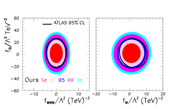
Figure 1: Allowed regions in the planes $f_{B}/\Lambda^{2}\otimes f_{WWW}/\Lambda^{2}$ (left panel) and $f_{B}/\Lambda^{2}\otimes f_{W}/\Lambda^{2}$ (right panel) at $1\sigma$, 95%, 99%, and $3\sigma$ CL. The black line stands for the border of the 95% CL allowed region obtained by ATLAS Aad et al. (2016a).

When including the effect of the additional operators we must also account for their contribution to the EWPD. Our construction of the $\chi^{2}$ function for the EWPD follows the analysis in Ref. Corbett et al. (2017) to which we refer the reader for details. In brief in our EWPD analysis we fit 15 observables of which 12 are $Z$ observables Schael et al. (2006):

$$\Gamma_{Z}\;\;,\;\;\sigma_{h}^{0}\;\;,\;\;{\cal A}_{\ell}(\tau^{\rm pol})\;\;,\;\;R^{0}_{\ell}\;\;,\;\;{\cal A}_{\ell}({\rm SLD})\;\;,\;\;A_{\rm FB}^{0,l}\;\;,\;\;R^{0}_{c}\;\;,\;\;R^{0}_{b}\;\;,\;\;{\cal A}_{c}\;\;,\;\;{\cal A}_{b}\;\;,\;\;A_{\rm FB}^{0,c}\;\;,\;\;\hbox{ and}\;\;A_{\rm FB}^{0,b}\hbox{ (SLD/LEP-I)}\;\;\;,$$

complemented by three $W$ observables

$$M_{W}\;\;,\;\;\Gamma_{W}\;\;\hbox{ and}\;\;\hbox{Br}(W\to{\ell\nu})$$

that are, respectively, its average mass taken from Patrignani et al. (2016), its width from LEP2/Tevatron Group (2010), and the leptonic $W$ branching ratio for which the average in Ref. Patrignani et al. (2016) is considered. The correlations among these inputs are presented in Ref. Schael et al. (2006) and we take them into consideration in the analyses. The SM predictions and their uncertainties due to variations of the SM parameters were extracted from Ciuchini et al. (2014).

Altogether we construct a combined $\chi^{2}$ function

$$\chi^{2}_{\rm LHC-RI\,+\,EWPD} \equiv \chi^{2}_{\rm LHC-RI}(f_{W},f_{B},f_{WWW},f_{BW},f_{\Phi,1},f^{(1)}_{\phi,Q},f^{(3)}_{\phi,Q},f^{(1)}_{\phi,u},f^{(1)}_{\phi,d})$$ (21)

$$+ \chi^{2}_{\rm EWPD}(f_{BW},f_{\Phi,1},f^{(1)}_{\phi,Q},f^{(3)}_{\phi,Q},f^{(1)}_{\phi,u},f^{(1)}_{\phi,d},f^{(1)}_{\phi,e},f_{LLLL})\;,$$

from which we derive the allowed ranges for each coefficient or pair of coefficients after marginalization over all the others. It is worth commenting that this marginalization of the profiled binned log-likelihood is computationally very expensive due the high dimensionality of the parameters space. Achieving an acceptable accuracy in the determination of the statistical confidence bounds for one- and two-dimensional distributions requires typically hundreds of millions of Monte Carlo evaluations for each one of the points used to obtain the 1D and 2D the allowed regions.

Finally, for comparison, we also consider the constraints from LEP2 global analysis of TGC The LEP Collaborations ALEPH, DELPHI, L3, OPAL, and the LEP TGC Working Group . In order to do so we follow the procedure in Ref. Butter et al. (2016) and construct a simplified gaussian $\chi^{2}_{\rm LEP2}$ using the central values, $\sigma$ and correlation matrix for the couplings $\Delta g^{1}_{Z}$, $\Delta\kappa_{\gamma}$ and $\lambda$ and their correlation coefficients from the final combined LEP2 analysis in Ref. The LEP Collaborations ALEPH, DELPHI, L3, OPAL, and the LEP TGC Working Group (reproduced in Table 1 for completness) which was performed in terms of these effective TGC coefficients under the relations implied by dimension-six effective operator formalism for TGC. We notice, however, that in extracting those bounds on the effective TGC couplings, the LEP collaborations did not include the effect of fermion operators. For that reason the combination of those LEP2 bounds with our LHC Run I and EWPD is only shown for the purpose of illustration.

	LEP
	xxxxxx 68 % CL xxxxxx	Correlations
$\Delta g_{1}^{Z}$	$-$ $0.051^{+0.031}_{-0.032}$	$1.00$	$0.23$	$-0.30$
$\Delta\kappa_{\gamma}$	$-0.067^{+0.061}_{-0.057}$	$0.23$	$1.00$	$-0.27$
$\lambda$	$-0.067^{+0.036}_{-0.038}$	$-0.30$	$0.27$	$1.00$

Table 1: $\Delta g_{1}^{Z}$, $\Delta\kappa_{\gamma}$ and $\lambda$ central values, standard deviations and correlation coefficients from LEP2 The LEP Collaborations ALEPH, DELPHI, L3, OPAL, and the LEP TGC Working Group .

IV BOUNDS ON TRIPLE GAUGE BOSON INTERACTIONS

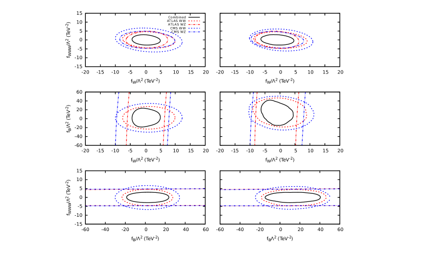
Figure 2: Allowed 95% CL regions in the planes $f_{WWW}/\Lambda^{2}\otimes f_{B}/\Lambda^{2}$ (top row), $f_{B}/\Lambda^{2}\otimes f_{W}/\Lambda^{2}$ (middle row) and $f_{WWW}/\Lambda^{2}\otimes f_{W}/\Lambda^{2}$ (lower row) for the different channels as labeled in the figure. In the left panels only $f_{WWW}$, $f_{W}$ and $f_{B}$ were considered non-zero in the fit, while the right panels display the result from the 11 parameter fit. In each case we marginalize over the undisplayed non-zero variables.

We start by showing the results of our analysis in terms of the allowed ranges for the Wilson coefficients of the three “canonical” TGC operators, $f_{WWW}/\Lambda^{2}$, $f_{W}/\Lambda^{2}$ and $f_{B}/\Lambda^{2}$. We depict first in Fig. 2 the 95% CL (2 dof) allowed regions in the planes $f_{B}/\Lambda^{2}\otimes f_{W}/\Lambda^{2}$, $f_{WWW}/\Lambda^{2}\otimes f_{B}/\Lambda^{2}$ and $f_{WWW}/\Lambda^{2}\otimes f_{W}/\Lambda^{2}$ for the $W^{+}W^{-}$ and $W^{\pm}Z$ channels and for ATLAS and CMS, as well as the combination of these results. In order to assess the impact of additional operators in the TGC extraction at LHC we performed first the “standard” analysis fitting just these three coefficients, and setting the coefficient of all other operators to zero. The corresponding allowed regions are shown in the left panels after marginalizing over the third coefficient which is not displayed. Conversely the results of the global analysis of the LHC Run I data together with EWPD performed in terms of 11 non-zero Wilson coefficients (see Eq. (7)) are shown on the right panels. These regions are obtained after marginalization over the 9 undisplayed coefficients.

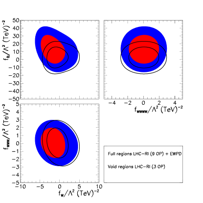
Figure 3: $1\sigma$ and 95% CL allowed regions in the planes indicated in the axes. Here we considered the $W^{+}W^{-}$ and $W^{\pm}Z$ productions and the EWPD in the analyses. The data set and parameters used are as indicated in the figure.

One salient feature of Figure 2 is that the $W^{\pm}Z$ bounds on the Wilson coefficient $f_{B}/\Lambda^{2}$ are much looser than the ones on $f_{W}/\Lambda^{2}$ and $f_{WWW}/\Lambda^{2}$ , as expected, because ${\cal O}_{B}$ does not contribute to the leading term of the growth of the scattering amplitudes; see Eqs. (14)–(20).

For better comparison of the results obtained with and without including the additional operators we overlay in Fig. 3 the $1\sigma$ and 95% CL allowed regions obtained combining all channels and experiments for the two scenarios. As we can see from this figure the addition of more parameters leads to the expansion of the allowed regions, as expected. Moreover, the region of $f_{B}/\Lambda^{2}$ suffers the largest shift towards positive values of this parameter while there is a small shift in the $f_{W}/\Lambda^{2}$ direction and there is no appreciable displacement along the $f_{WWW}/\Lambda^{2}$ axis.

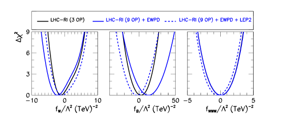
Figure 4: $\Delta\chi^{2}$ dependence on the $f_{W}/\Lambda^{2}$ (left panel), $f_{B}/\Lambda^{2}$ (central panel) and $f_{W}/\Lambda^{2}$ (right panel) parameters after the marginalization over the remaining fit parameters. The solid black line stands for the standard TGC analysis, while the solid blue line represents the 9 parameter fit to the LHC Run I data and the EWPD. The dashed blue line differs from the solid ones just by the addition of LEP2 data on TGC.

The corresponding dependence of the $\Delta\chi^{2}$ for the two analysis with each of the three coefficients is given in Fig. 4 and from those we read the 95%CL one-dimensional allowed ranges for each coefficient given in Table 2. As seen above, the $\Delta\chi^{2}$ distribution for $f_{B}/\Lambda^{2}$ ($f_{W}/\Lambda^{2}$) broadens and shifts to positive (negative) values when we compare the results considering only the LHC Run I data and three canonical parameters (solid black line) with the one containing additional operators also constrained by the EWPD (solid blue line). Quantitatively the effect is slightly larger for $f_{B}/\Lambda^{2}$ whose allowed range widens by about 30% versus 20% for $f_{W}/\Lambda^{2}$.

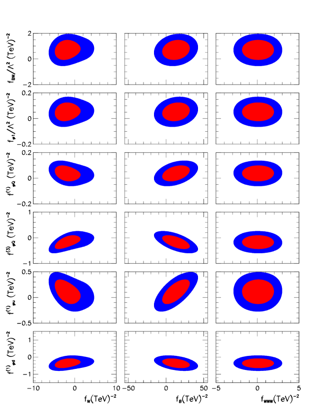
Figure 5: $1\sigma$ and 95% CL allowed regions in the planes indicated in the axes. Here we considered the $W^{+}W^{-}$ and $W^{\pm}Z$ productions and the EWPD in the analyses.

The effect of each of the six additional operators on the extracted range of the three “canonical” TGC operator coefficients is illustrated in Figure 5 where we depict the two-dimensional correlations between the three TGC coefficients and the additional ones. In each panel of this figure we exhibit the $1\sigma$ and 95% CL level (2 dof) allowed regions after marginalizing over the remaining parameters. As we can see, $f_{B}/\Lambda^{2}$ has a significant correlation only with $f^{(1)}_{\Phi u}/\Lambda^{2}$ and to a lesser extent is (anti-) correlated with $f^{(1)}_{\Phi Q}/\Lambda^{2}$ ($f^{(3)}_{\Phi Q}/\Lambda^{2}$ and $f^{(1)}_{\Phi d}/\Lambda^{2}$). This is expected as these are the operator coefficients contributing the growth of the scattering amplitudes into longitudinally polarized gauge bosons (Eqs. 14– 20). In particular the correlion with $f^{(1)}_{\Phi u}/\Lambda^{2}$ can be understood from the scattering amplitude in Eq. (18). Similarly $f_{W}/\Lambda^{2}$ shows a stronger anti-correlation only with $f^{(1)}_{\Phi u}/\Lambda^{2}$ and to a smaller degree is correlated with $f^{(3)}_{\Phi Q}/\Lambda^{2}$ and $f^{(1)}_{\Phi d}/\Lambda^{2}$. Finally from the third column of this figure we can see that $f_{WWW}/\Lambda^{2}$ shows no correlation with the additional parameters as expected since ${\cal O}_{WWW}$ contributes by itself to the energy growth of the scattering amplitudes for transversely polarized gauge bosons.

The impact of the LHC diboson production data on the determination of the parameters directly constrained by the EWPD is illustrated in Fig. 6 that depicts the $\Delta\chi^{2}$ distribution as a function of these parameters where the magenta (blue) line stands for the result obtained using the EWPD (and the LHC Run I diboson production data).

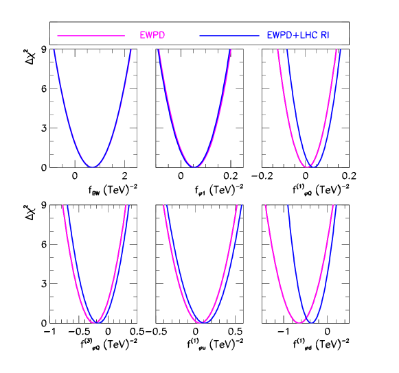
Figure 6: $\Delta\chi^{2}$ dependence on the $f_{BW}/\Lambda^{2}$, $f_{\Phi 1}/\Lambda^{2}$, $f^{(1)}_{\Phi Q}/\Lambda^{2}$, $f^{(3)}_{\Phi Q}/\Lambda^{2}$, $f^{(1)}_{\Phi u}/\Lambda^{2}$, and $f^{(1)}_{\Phi d}/\Lambda^{2}$ after the marginalization over the undisplayed parameters. The magenta line stands for the results using only the EWPD while the blue one is obtained considering the EWPD and LHC Run I diboson production.

The top left and middle panels of this figure show that the addition of the LHC data does not alter the constraints on $f_{BW}/\Lambda^{2}$ and $f_{\Phi 1}/\Lambda^{2}$ parameters. This is easy to understand since these parameters do not modify the high energy behavior of $q\bar{q}\to VV$ amplitudes; see Eqs. (14)–(15). This is expected from ${\cal O}_{\Phi,1}$ as it only contributes to the amplitudes via finite renormalization effects of the SM parameters. The operator ${\cal O}_{BW}$, on the other hand, modifies the TGC directly also, however, its effects on the $Z$ wave-function renormalization cancel the growth with the center–of–mass energy due to the anomalous TGC. From the top right, bottom left and middle panels we can see that the impact of the Run I data on $f^{(1)}_{\Phi Q}/\Lambda^{2}$, $f^{(3)}_{\Phi Q}/\Lambda^{2}$ and $f^{(1)}_{\Phi u}/\Lambda^{2}$ is marginal. $f^{(1)}_{\Phi d}/\Lambda^{2}$ is the only parameter whose $\Delta\chi^{2}$ distribution gets significantly affected. The EWPD analysis favours non-vanishing value for $f^{(1)}_{\Phi d}/\Lambda^{2}$ at 2$\sigma$, a result driven by the 2.7$\sigma$ discrepancy between the observed $A_{\rm FB}^{0,b}$ and the SM. On the contrary no significant discrepancy is observed between the observed LHC Run I diboson data and the SM. Hence there is a shift towards zero of $f^{(1)}_{\Phi d}/\Lambda^{2}$ when including the LHC Run I data in the analysis. This slight tension results also into the reduction of the globally allowed range.

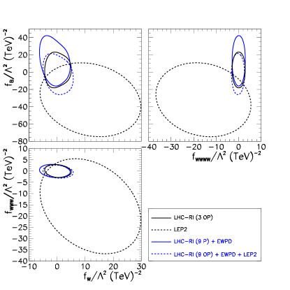
Figure 7: Two-dimensional 95% CL allowed regions in the planes indicated in the axes. Here we considered the $W^{+}W^{-}$ and $W^{\pm}Z$ productions, LEP2 data on TGC and the EWPD in the analyses. The lines are as shown in the figure.

We finish this section by comparing our results with the bounds derived from LEP2 diboson data. To do so we plot in Figure 7 the two-dimensional 95% CL allowed regions for the three combination of the canonical TGC parameters for the analysis with and without additional operators together with the LEP2 results. As shown in Ref.Butter et al. (2016), the limits emanating from the canonical LHC Run I diboson data (black solid line) are substantially more stringent than those imposed by LEP2 (black dashed line). As seen in this figure, enlarging the number of operators in the LHC analyses, together with the EWPD, does not alter this conclusion despite the growth of the allowed regions (solid blue line). For illustration we also show in the figure the allowed regions obtained by naively combining the general LHC Run I + EWPD analysis with the LEP2 information (see discussion at the end of Sec. III). As seen, including LEP2 data in the approximation used leads to a reduction of the allowed regions in the $f_{B}/\Lambda^{2}$ direction, as well as to a shift of it towards negative values (see also the dashed blue line in Fig. 4).

V Summary

In this work we have quantified the impact of possible anomalous gauge couplings to quarks on the TGC determination performed using the LHC Run I diboson data. In order to carry out a statistically consistent analysis we have included in addition the EWPD to constrain the couplings between quarks and gauge boson as well as the modifications of the gauge boson self energies. We have worked in the framework of effective Lagrangians so our study has been performed including the 11 dimension-six operators given in Eq. (7).

As a summary of our findings we present in Table 2 the 95% CL globally allowed ranges for the Wilson coefficients of the nine operators that contribute to the LHC Run I data considered. The comparison of the the first and third columns of this table shows that the addition of the new operators modifies the TGC bounds on $f_{B}/\Lambda^{2}$ and $f_{W}/\Lambda^{2}$ coming from the LHC Run I diboson. Quantitatively the effect is slightly larger for $f_{B}/\Lambda^{2}$ whose allowed range widens by about 30% versus 20% for $f_{W}/\Lambda^{2}$. The limits on $f_{WWW}/\Lambda^{2}$, on the contrary, result almost unaffected. Despite these changes, the constraints on these parameters are still dominated by the LHC Run I data at large, and are still substantially stronger than those obtained from LEP2 data.

We have also learned from our analyses that the LHC Run I diboson data is not precise enough to yield substantial information on the gauge couplings to quarks in addition to what is already known from EWPD; contrast the second and third columns of Table 2. The only apparent exception is $f^{(1)}_{\Phi d}/\Lambda^{2}$ which in the considered family universal scenario is driven to be non-zero in the EWPD analysis by the discrepancy between the measured $A_{\rm FB}^{0,b}$ at LEP/SLC and the SM while LHC Run I data shows no evidence of any deviation with respect to the SM. Nevertheless, these results allow us to foresee that diboson production at the LHC will play an important role in the analyses of anomalous couplings of gauge bosons to quarks as the LHC increases the integrated luminosity. Hence global analysis of LHC and EWPD are becoming a must for consistent determination of the Wilson coefficients of the full set of dimension-6 operators.

coupling	95% allowed range (TeV${}^{-2})$
	LHC RI (3 OP)	EWPD	LHC RI (9 OP) + EWPD
$f_{W}$	$(-3.9\,,\,3.9)$	—	$(-5.6\,,\,4.0)$
$f_{B}$	$(-15\,,\,20)$	—	$(-11\,,\,37)$
$f_{WWW}$	$(-2.4\,,\,2.5)$	—	$(-2.4\,,\,2.6)$
$f_{BW}$	—	$(-0.32\,,\,1.7)$	$(-0.33\,,\,1.7)$
$f_{\Phi 1}$	—	$(-0.040\,,\,0.15)$	$(-0.044\,,\,0.15)$
$f^{(1)}_{\Phi Q}$	—	$(-0.083\,,\,0.10)$	$(-0.044\,,\,0.12)$
$f^{(3)}_{\Phi Q}$	—	$(-0.60\,,\,0.12)$	$(-0.52\,,\,0.18)$
$f^{(1)}_{\Phi u}$	—	$(-0.25\,,\,0.37)$	$(-0.19\,,\,0.42)$
$f^{(1)}_{\Phi d}$	—	$(-1.2\,,\,-0.13)$	$(-0.73\,,\,0.023)$

Table 2: 95% CL allowed ranges for the Wilson coefficients of the dimension–six operators that contribute to the studied processes in gauge boson pair production at LHC. The ranges for each parameter are obtained after marginalization of the coefficients of all other operators contributing to each analysis. In particular the results given in the third and forth column are obtain after marginalization over $f^{(1)}_{\phi,e}$ and $f_{LLLL}$ as well.