Self-Joinings for 3-IETs

Abstract.

We show that typical interval exchange transformations on three intervals are not 2-simple answering a question of Veech. Moreover, the set of self-joinings of almost every 3-IET is a Paulsen simplex.

1. Introduction

Defintion 1.

Let $(X,\mathcal{B},\mu,T)$ be a probability measure preserving system. A self-joining is a $T\times T$ invariant measure on $X\times X$ with marginals $\mu$.

Defintion 2.

$(X,\mathcal{B},\mu,T)$ is called 2-simple if every ergodic self-joining, other than $\mu\times\mu$, is one-to-one on almost every fiber.

Defintion 3.

A Poulsen simplex is a metrizable simplex where the extreme points are dense.

Lindenstrauss, Olsen and Sternfeld proved that a Poulsen simplex is unique up to affine homeomorphism [10].

Defintion 4.

a 3-interval exchange transformation is defined by 3 non-negative numbers $\ell_{1},\ell_{2},\ell_{3}$. It is $T:[0,\ell_{1}+\ell_{2}+\ell_{3})\to[0,\ell_{1}+\ell_{2}+\ell_{3})$ by

$$T(x)=\begin{cases}x+\ell_{2}+\ell_{3}&\text{if $x\leq\ell_{1}+\ell_{2}$}\\ x+\ell_{2}+\ell_{3}-(\ell_{1}+2\ell_{2}+\ell_{3})&\text{otherwise.}\end{cases}$$

Theorem 1.1.

Almost every 3-IET is not 2-simple. Also, its self-joinings form a Poulsen simplex.

Note that $T\times T$ has topological entropy 0.

The first part of Theorem 1.1 answers a question of Veech in the negative [15, Question 4.9]. (In [15] “$2$-simple” is called “Property $S$.”)

Recall that a measure preserving system is called prime if it has no non-trivial factors. In the paper [15] mentioned above, Veech classified the factors of $2$-simple systems, and so a natural question remains:

Question 1.

Is almost every 3-IET prime?

It is also natural to wonder what happens for IETs with other permutations and flows on translation surfaces. It is likely that our techniques can show that residual sets of interval exchange transformations on more intervals, and flows on translation surfaces of genus greater than 1 are not simple, but we do not see how they can be applied to almost every flow on translation surface or IET with different permutation.

To prove Theorem 1.1 we define in Section 2 a distiguished class of self-joinings called “shifted power joinings.” In Section 2 we also show that a special type of transformations called “rigid rank 1 by intervals” (which includes IET’s by [16, Part 1, Theorem 1.4 ]) have the property that linear combinations of shifted power joinings are dense in their self-joinings. M. Lemanczyk brought to our attention that this result was proved in an unpublished paper of J. King [9]. We then prove that almost every 3-IET has the property that its ergodic self-joinings are dense in linear combinations of the shifted power joinings. We do this by having an abstract criterion (Section 3) and showing 3-IETs verify this criterion (Section 4).

Context of our results: Before Veech’s work, D. Rudolph introduced the notion of minimal self joinings, using it as a fruitful class of examples, including examples of prime systems [11]. The property of 2-simple generalizes minimal self joinings and in particular, no rigid system has minimal self joinings. The typical IET is rigid [16, Part 1, Theorem 1.4], so the typical IET does not have minimal self joinings, but there are rigid 2 simple systems. Ageev proved that the set of measure preserving transformations which are not 2 simple contains a dense $G_{\delta}$, i.e. it is a residual set, (with the topology being the so called weak topology) [1]. Our construction can be modified to give a new proof of this fact.

Our result that the self-joinings form a Paulsen simplex is also perhaps a little unexpected. Many examples of systems whose set of invariant measures form a Paulsen simplex are well known, but typically these systems are high complexity, satisfying some form of specification. In contrast, our examples have very low complexity, as $T\times T$ has quadratic block growth. Since systems of linear block growth have only finitely many ergodic measures [2], such a system can not have that the set of its invariant measures form a Paulsen simplex (though as our examples show its Cartesian product could). We remark that in the previously mentioned unpublished work, J. King proved a residual set of measure preserving transformations (which therefore must include rank 1 transformations) have that their set of their self-joinings form a Paulsen simplex [9], giving many (non-explicit) entropy zero examples. Our result is perhaps still surprising, because we treat a previously considered family of examples and we show typicality in a metric, rather than topological setting.

Two key steps are showing that the typical 3-IET admit $(n_{j},n_{j}+1)$ approximation (see the proof of Proposition 4.5) and that this implies the existence of all sorts of ergodic joinings (see Proposition 3.1). Some consequences of transformations with $(n_{j},n_{j}+1)$ approximation were studied by Ryzhikov [13] and as a result we get some spectral consequences for $T^{n}$ and $\underbrace{T\times...\times T}_{n\text{ times}}$, see Remark 2.

Acknowledgments: We thank El Abdaloui, M. Lemaczyk and V. Ryzhikov for numerous illuminating discussions on connections of other results with this work.

2. Joinings of rigid rank 1 transformations come from limits of linear combinations of powers

Let $([0,1],\mathcal{M},\lambda,T)$ be an ergodic invertible transformation.

Defintion 5.

We say $T$ is rigid rank 1 by intervals if there exists a sequence of intervals $I_{1},\dots$ and natural numbers $n_{1},\dots$ so that

• $T^{i}I_{k}$ is an interval with $diam(T^{i}I_{k})=diam(I_{k})$ for all $0\leq i<n_{k}$.

• $T^{i}I_{k}\cap T^{j}I_{k}=\emptyset$ for all $k$ and $0\leq i<j<n_{k}$.

• $\underset{k\to\infty}{\lim}\lambda(\cup_{i=0}^{n_{k}-1}T^{i}I_{k})=1$.

• $\underset{k\to\infty}{\lim}\frac{\lambda(T^{n_{k}}I_{k}\Delta I_{k})}{\lambda(I_{k})}=0$.

This is a condition saying that our transformation is well approximated by periodic transformations. A similar condition, admiting cyclic approximation by periodic transformations was considered in [6].

Let

$${\mathcal{R}}_{k}=\bigcup_{i=0}^{n_{k}-1}T^{i}I_{k},$$

(2.1) $$\hat{{\mathcal{R}}}_{k}=\bigcup_{i=0}^{n_{k}-1}T^{i}(I_{k}\cap T^{-n_{k}}I_{k}\cap T^{n_{k}}I_{k}),$$

$$\tilde{{\mathcal{R}}}_{k}=\bigcup_{i=0}^{n_{k}-1}T^{i}(I_{k}\cap T^{-n_{k}}I_{k}\cap T^{-2n_{k}}I_{k}\cap T^{n_{k}}I_{k}\cap T^{2n_{k}}I_{k}),$$

Then, ${\mathcal{R}}_{k}$ is the Rokhlin tower over $I_{k}$, $\hat{{\mathcal{R}}}_{k}$ is the Rokhlin tower over $I_{k}\cap T^{-n_{k}}I_{k}\cap T^{n_{k}}I_{k}$, and $\tilde{{\mathcal{R}}}_{k}$ is the Rokhlin tower over $\bigcap_{i=-2}^{2}T^{in_{k}}I_{k}$. We have

(2.2) $$\hat{{\mathcal{R}}}_{k}=\{x:T^{i}x\in{\mathcal{R}}_{k}\text{ for all }-n_{k}<i<n_{k}\},$$

and

(2.3) $$\tilde{{\mathcal{R}}}_{k}=\{x:T^{i}x\in{\mathcal{R}}_{k}\text{ for all }-2n_{k}<i<2n_{k}\}.$$

Heuristically one can think of ${\mathcal{R}}_{k}$ as the set of points we can control. $\hat{{\mathcal{R}}}_{k}$ and $\tilde{{\mathcal{R}}}_{k}$ let us control the points for long orbit segments, which is necessary for some of our arguments.

Lemma 2.1.

$\underset{k\to\infty}{\lim}\lambda(\tilde{{\mathcal{R}}}_{k})=1=\underset{k\to\infty}{\lim}\lambda({\mathcal{R}}_{k})=\underset{k\to\infty}{\lim}\lambda(\hat{{\mathcal{R}}}_{k})$.

Proof.

By the third condition in the definition of rigid rank 1 by intervals we have $\underset{k\to\infty}{\lim}\lambda({\mathcal{R}}_{k})=1$. By (2.1),

$$\lambda(\hat{{\mathcal{R}}}_{k})\geq\lambda({\mathcal{R}}_{k})-n_{k}\lambda(I_{k}\setminus(T^{n_{k}}I_{k}\cup T^{-n_{k}}I_{k}))\geq\lambda({\mathcal{R}}_{k})-2n_{k}\lambda(I_{k}\setminus T^{n_{k}}I_{k}),$$

and thus by the fourth condition of the definition of rigid rank 1 by intervals, $\underset{k\to\infty}{\lim}\lambda(\hat{{\mathcal{R}}}_{k})\to 1$. Similarly, $\underset{k\to\infty}{\lim}\lambda(\tilde{R}_{k})=1$. ∎

Defintion 6 (Shifted Power Joining).

Let $(X,T,\mu)$ be a measure preserving dynamical system. A self-joining of $(X,T,\mu)$ that gives full measure to $\{(x,T^{a}x)\}$ for some $a\in{\mathbb{Z}}$ with $a\neq 0$ is called a shifted power joining.

These have also been called off diagonal joinings.

Let $\iota:[0,1]\to[0,1]$ by $x\to(x,x)$. Let $\mu=\iota_{*}\lambda$. Shifted power joinings have the form $(id\times T^{a})_{*}\mu$ for some $a\in\mathbb{Z}\setminus\{0\}$.

The operator $A_{\sigma}$ and convergence in the strong operator topology. Let $\sigma$ be a self-joining of $(T,\lambda)$. Let $\sigma_{x}$ be the corresponding measure on $[0,1]$ coming from disintegrating along $\sigma$ on the fiber $\{x\}\times[0,1]$. Define $A_{\sigma}:L^{2}(\lambda)\to L^{2}(\lambda)$ by $A_{\sigma}(f)[x]=\int fd\sigma_{x}$.

Recall that one calls the strong operator topology the topology of pointwise convergence on $L^{2}(\lambda)$. That is $A_{1},...$ converges to $A_{\infty}$ in the strong operator topology if and only if $\underset{i\to\infty}{\lim}\|A_{i}f-A_{\infty}f\|_{2}=0$ for all $f\in L^{2}(\lambda)$.

Theorem 2.2.

Assume $([0,1],T,\lambda)$ is rigid rank 1 by intervals and $\sigma$ is a self-joining of $([0,1],T,\lambda)$. Then $A_{\sigma}$ is the strong operator topology (SOT) limit of linear combinations, with non-negative coefficients, of powers of $U_{T}$, where $U_{T}:L^{2}([0,1],\lambda)\to L^{2}([0,1],\lambda)$ denotes the Koopman operator $U_{T}(f)=f\circ T$.

Corollary 2.3.

(J. King) Any self-joining of a rigid rank 1 by intervals transformation is a weak-* limit of linear combinations of shifted power joinings.

These results (or very closely related results) were established earlier by J. King [9] using a different proof. In fact he shows that if the joining in Corollary 2.3 is ergodic then there is no need to take a linear combination. See also [5, Theorem 7.1]. There is an open question of whether this result is true for general rank 1 systems [8, Page 382]. Ryzhikov has a series of results in this direction, see for example [12] and [14].

2.1. Proof of Theorem 2.2

Lemma 2.4.

For each $0\leq j<n_{k}$ we have

(2.4) $$n_{k}\int_{T^{j}I_{k}}\sigma_{x}({\mathcal{R}}_{k}^{c})d\lambda(x)\leq\lambda(\tilde{{\mathcal{R}}}_{k}^{c}).$$

Remark. Note that $n_{k}$ is roughly $\lambda(T^{j}I_{k})^{-1}$.

Proof.

Suppose $0\leq j<n_{k}$, and suppose $x\in T^{j}I_{k}$. From (2.3) we have $T^{i}{\mathcal{R}}_{k}^{c}\subset\tilde{{\mathcal{R}}}_{k}^{c}$ for all $-n_{k}<i<n_{k}$. We claim that

(2.5) $$\sigma_{x}({\mathcal{R}}_{k}^{c})\leq\sigma_{T^{\ell}x}(\tilde{{\mathcal{R}}}_{k}^{c})\qquad\text{for all $-n_{k}<\ell<n_{k}$.}$$

Indeed, $\sigma_{x}({\mathcal{R}}^{c}_{k})=\sigma_{T^{\ell}x}(T^{\ell}{\mathcal{R}}^{c}_{k})\leq\sigma_{T^{\ell}x}(\tilde{{\mathcal{R}}}_{k}^{c})$, proving (2.5). Integrating (2.5) we get

(2.6) $$\int_{T^{j}I_{k}}\sigma_{y}({\mathcal{R}}_{k}^{c})d\lambda(y)\leq\int_{T^{j+\ell}I_{k}}\sigma_{z}(\tilde{{\mathcal{R}}}_{k}^{c})d\lambda(z)\quad\text{for all $-n_{k}<\ell<n_{k}$.}$$

Since we can choose $\ell$ in (2.6) so that $j+\ell$ takes any value in $[0,n_{k}-1]\cap{\mathbb{Z}}$, we get

(2.7) $$\int_{T^{j}I_{k}}\sigma_{y}({\mathcal{R}}_{k}^{c})d\lambda(y)\leq\min_{0\leq i<n_{k}}\int_{T^{i}I_{k}}\sigma_{z}(\tilde{{\mathcal{R}}}_{k}^{c})d\lambda(z).$$

Now

$$\sum_{i=0}^{n_{k}-1}\int_{T^{i}I_{k}}\sigma_{y}(\tilde{{\mathcal{R}}}_{k}^{c})d\lambda(y)\leq\int_{[0,1]}\sigma_{y}(\tilde{{\mathcal{R}}}_{k}^{c})d\lambda(y)\leq\lambda(\tilde{{\mathcal{R}}}_{k}^{c}),$$

where the last estimate uses that $\sigma$ has projections $\lambda$. So we obtain

(2.8) $$\min\limits_{0\leq i<n_{k}}\int_{T^{i}I_{k}}\sigma_{x}(\tilde{{\mathcal{R}}}_{k}^{c})d\lambda(x)\leq\frac{1}{n_{k}}\lambda(\tilde{{\mathcal{R}}}_{k}^{c}).$$

Now the estimate (2.4) follows from (2.7) and (2.8). ∎

We want to guess coefficients $c_{j}$ so that $\sigma$ is close to $\sum_{j=0}^{n_{k}-1}c_{j}(id\times T^{i})_{*}\mu$. The next lemma comes up with a candidate pointwise version. Theorem 2.2 and Corollary 2.3 follow because by Egoroff’s theorem this choice is almost constant on most of the $T^{\ell}I_{k}$ and the lemma after this (Lemma 2.6), which shows that they are almost $T$ invariant.

Lemma 2.5.

Let $x\in\hat{{\mathcal{R}}}_{k}\cap T^{j}I_{k}$ where $0\leq j<n_{k}$. Define $c_{i}(x)=\sigma_{x}(T^{a}I_{k}\cap\hat{{\mathcal{R}}}_{k})$ where $0\leq a<n_{k}$ and $i+j\equiv a\,(\text{mod }n_{k})$. For all 1-Lipschitz $f$ we have

$$\left|A_{\sigma}f(x)-\sum_{i=0}^{n_{k}-1}c_{i}(x)f(T^{i}x)\right|\leq\operatorname{diam}(I_{k})+2\|f\|_{\sup}\sigma_{x}(\hat{{\mathcal{R}}}_{k}^{c}).$$

Morally $c_{j}(x)$ is the $\sigma_{x}$ measure of the level in $R_{k}$ that is $j$ levels above the level $x$ is on. Because $j+\ell$ can be bigger than $n_{k}$ the definition is slightly more complicated. Note that the $c_{j}(x)$ are non-negative.

Proof.

Suppose $x\in\hat{{\mathcal{R}}}_{k}\cap T^{j}I_{k}$. First notice that if $y,z\in T^{i}I_{k}$ for some $0\leq i<n_{k}$ we have that $d(y,z)<\operatorname{diam}(I_{k})$. So if $j+\ell<n_{k}$ we have

(2.9) $$\left|\int_{\hat{R}_{k}\cap T^{j+\ell}I_{k}}fd\sigma_{x}-c_{j}(x)f(T^{i}x)\right|\leq\|f\|_{Lip}\,\operatorname{diam}(I_{k}).$$

If $j+\ell\geq n_{k}$ then $|c_{j}(x)-\lambda(\hat{R}_{k}\cap T^{j+\ell}I_{k})|\leq\lambda(\tilde{R}^{c}_{k}\cap T^{j+\ell}I_{k})$ because if $y\in\tilde{R}_{k}$ then $T^{\pm n_{k}}y\in\hat{R}_{k}$. So for any $j$ we have

(2.10) $$\left|\int_{\hat{R}_{k}\cap T^{j+\ell}I_{k}}fd\sigma_{x}-c_{j}(x)f(T^{j}x)\right|\leq\|f\|_{Lip}\,\operatorname{diam}(I_{k})+\|f\|_{\sup}\,\lambda(\tilde{R}_{k}^{c}\cap T^{j+\ell}I_{k}).$$

By (2.2), for all $0\leq\ell<n_{k}$, $T^{-\ell}\hat{R}_{k}\subset R_{k}$. Therefore, $\hat{R}_{k}\subset\bigcup_{i=\ell}^{\ell+n_{k}-1}T^{i}I_{k}$ for all $0\leq\ell<n_{k}$. By summing over the $j$ in (2.10) we obtain

(2.11) $$\left|\int_{\hat{R}_{k}}fd\sigma_{x}-\sum_{j=0}^{n_{k}-1}c_{i}(x)f(T^{i}x)\right|\leq\|f\|_{Lip}\,\operatorname{diam}(I_{k})+\|f\|_{\sup}\lambda(\tilde{R}_{k}^{c}).$$

In view of the fact that

(2.12) $$\left|\int_{\hat{R}_{k}^{c}}f\,d\sigma_{x}\right|\leq\|f\|_{\sup}\,\lambda(\tilde{R}^{c}_{k}),$$

we obtain the lemma. ∎

Lemma 2.6.

Suppose $0\leq\ell<n_{k}$. If $x\in T^{\ell}I_{k}$ and $-\ell\leq i<n_{k}-\ell$ then

$$\sum_{j=0}^{n_{k}-1}|c_{j}(x)-c_{j}(T^{i}x)|\leq 2\sigma_{x}(\tilde{R}_{k}^{c}).$$

Proof.

Suppose $0\leq\ell<n_{k}$, $0\leq j<n_{k}$, and $-\ell\leq i<n_{k}-\ell$. First note that if $0\leq m<n_{k}$ and $z\in T^{m}I_{k}\cap\hat{R}_{k}$ then by (2.1), we have $T^{s}z\in T^{m+s}I_{k}\cap\hat{R}_{k}$ for all $-m\leq s<n_{k}-m$. Thus, if $j+\ell<n_{k}$ and $i+j+\ell<n_{k}$, we have

$$\sigma_{T^{i}x}(T^{i+j+\ell}I_{k}\cap\hat{R}_{k})=\sigma_{x}(T^{j+\ell}I_{k}\cap T^{-i}\hat{R}_{k})=\sigma_{x}(T^{j+\ell}I_{k}\cap\hat{R}_{k}).$$

This gives $c_{j}(x)=c_{j}(T^{i}x)$ if $j+\ell<n_{k}$ and $i+j+\ell<n_{k}$. By similar reasoning we have that $c_{j}(x)=c_{j}(T^{i}x)$ if $j+\ell\geq n_{k}$ and $i+j+\ell\geq n_{k}$.

Now lets assume that $j+\ell<n_{k}$ and $i+j+\ell\geq n_{k}$. Then,

(2.13) $$c_{j}(T^{i}x)=\sigma_{T^{i}x}(T^{i+j+\ell-n_{k}}I_{k}\cap\hat{R}_{k})=\sigma_{x}(T^{j+\ell-n_{k}}I_{k}\cap T^{-i}\hat{R}_{k}).$$

Also,

(2.14) $$c_{j}(x)=\sigma_{x}(T^{j+\ell}I_{k}\cap\hat{R}_{k}).$$

Now because $\tilde{R}_{k}\subset\bigcap_{i=-{n_{k}}}^{n_{k}}T^{i}\hat{R}_{k}$, if $z\in T^{i+j+\ell-n_{k}}I_{k}\cap\tilde{R}_{k}$, then, $z\in T^{j+\ell-n_{k}}I_{k}\cap T^{-i}\hat{R}_{k}$, and $z\in T^{j+\ell}I_{k}\cap\hat{R}_{k}$. Therefore, the symmetric difference between $T^{j+\ell-n_{k}}I_{k}\cap T^{-i}\hat{R}_{k}$ and $T^{j+\ell}I_{k}\cap\hat{R}_{k}$ is contained in the union of $T^{i+j+\ell-n_{k}}I_{k}\cap\tilde{R}_{k}^{c}$ and $T^{j+\ell}I_{k}\cap\tilde{R}_{k}^{c}$. Thus, in view of (2.13), and (2.14),

$$|c_{j}(x)-c_{j}(T^{i}x)|\leq\sigma_{x}(T^{j+\ell+i-n_{k}}\tilde{R}_{k}^{c})+\sigma_{x}(T^{j+\ell}\tilde{R}_{k}^{c}).$$

The last case, where $j+\ell\geq n_{k}$ and $0\leq i+j+\ell<n_{k}$ gives analogous bounds. So we bound $\sum_{i=0}^{n_{k}-1}|c_{j}(x)-c_{j}(T^{i}x)|$ by $2\sum_{i=0}^{n_{k}-1}\lambda(T^{i}I_{k}\cap\tilde{R}_{k}^{c})\leq 2\lambda(\tilde{R}_{k}^{c})$ and obtain the lemma. ∎

Let $d_{KR}$ denote the Kantorovich-Rubinstein metric on measures. That is

$$d_{KR}(\mu,\nu)=\sup\left\{\left|\int fd\mu-\int fd\nu\right|:f\text{ is 1-Lipschitz}\right\}.$$

The next lemma is an immediate consequence of this definition.

Lemma 2.7.

If $f$ is 1-Lipshitz and $d_{KR}(\sigma_{x},\sigma_{y})<\epsilon$ then $|A_{\sigma}f(x)-A_{\sigma}f(y)|<\epsilon$.

We say $0\leq j<n_{k}$ is k-good if there exists $y_{j}$ in $T^{j}I_{k}$ so that at least $1-\epsilon$ proportion of the points in $T^{j}I_{k}$ have their disintegration $\epsilon$ close to $y_{j}$. That is

$$\lambda(\{x\in T^{j}I_{k}\;\>:\;\>d_{KR}(\sigma_{x},\sigma_{y_{j}})<\epsilon\})\geq(1-\epsilon)\lambda(I_{k}).$$

Lemma 2.8.

For all $\epsilon>0$ there exists $k_{0}$ so that for all $k>k_{0}$ we have

$$|\{0\leq j<n_{k}:j\text{ is k-good }\}|>(1-\epsilon)n_{k}.$$

Proof.

By Lusin’s Theorem there exists a compact set $K$ of measure at least $1-\frac{\epsilon^{2}}{4}$ so that the map $y\to\sigma_{y}$ is continuous with respect to the usual metric on $[0,1]$ and the metric $d_{KR}$ on measures. Because $K$ is compact this map is uniformly continuous and so there exists $\delta>0$ so that $x,y\in K$ and $|x-y|<\delta$ then $d_{KR}(\sigma_{x},\sigma_{y})<\epsilon$. We choose $k$ so that $\operatorname{diam}(I_{k})<\delta$ and $\lambda([0,1]\setminus{\mathcal{R}}_{k})<\frac{\epsilon^{2}}{4}$. Let

$$\eta=\frac{1}{n_{k}}|\{0\leq j<n_{k}\;\>:\;\>\lambda(T^{j}I_{k}\cap K^{c})>\epsilon\lambda(I_{k})\}|.$$

Then, because the $T^{j}I_{k}$ are disjoint and of equal size and $\bigcup_{j=0}^{n_{k}-1}T^{j}I_{k}={\mathcal{R}}_{k}$, it is clear that

$$\eta\epsilon\leq\frac{\lambda(K^{c}\cap{\mathcal{R}}_{k})}{\lambda({\mathcal{R}}_{k})}\leq\frac{\frac{\epsilon^{2}}{4}}{1-\frac{\epsilon^{2}}{4}}<\frac{\epsilon^{2}}{2},$$

and thus $\eta<\epsilon/2$. This completes the proof of the lemma. ∎

Notation. If $j$ is $k$-good let

$$G_{j}=\{x\in T^{j}I_{k}:\lambda(\{y\in T^{j}I_{k}:d_{KR}(\sigma_{x},\sigma_{y})<2\epsilon\})>(1-\epsilon)\lambda(I_{k})\},$$

i.e. $G_{j}$ is the set of points that are almost continuity points of the map $x\to\sigma_{x}$ (restricted to $T^{j}I_{k}$). We set $G_{j}=\emptyset$ if $j$ is not $k$-good.

Lemma 2.9.

For all $\epsilon>0$ there exists $k_{1}$ so that for all $k>k_{1}$ there exists $0\leq\ell<n_{k}$ and $y_{k}\in T^{\ell}I_{k}\cap\hat{{\mathcal{R}}}_{k}$ so that $\sigma_{y_{k}}(\tilde{{\mathcal{R}}}_{k}^{c})<\epsilon$ and

(2.15) $$|\{-\ell\leq j<n_{k}-\ell:T^{j}y_{k}\in G_{\ell+j}\text{ and }j\text{ is $k$-good}\}|>(1-12\epsilon)n_{k}.$$

Proof.

If $j$ is $k$-good then

$$\lambda(G_{j})>(1-\epsilon)\lambda(I_{k}).$$

Let ${\mathcal{R}}_{k}^{*}=\bigcup_{j=0}^{n_{k}-1}G_{j}$. Notice that $\underset{k\to\infty}{\lim}\,\lambda(\cup_{i=0}^{n_{k}-1}T^{i}I_{k})=\underset{k\to\infty}{\lim}\,\lambda({\mathcal{R}}_{k})=1$ and so for all large enough $k$ (so that $\lambda({\mathcal{R}}_{k})$ is close to 1 and Lemma 2.8 holds) we have

$$\lambda({\mathcal{R}}_{k}^{*})\geq(1-\epsilon)^{2}\lambda({\mathcal{R}}_{k})>1-3\epsilon.$$

By a straightforward $L^{1}$ estimate, we have

$$\sum_{\ell=0}^{n_{k}-1}\lambda(\{y\in T^{\ell}I_{k}:|\{-\ell\leq j<n_{k}-\ell:G_{j}=\emptyset\text{ or }T^{j}y\not\in G_{j+\ell}\}|\geq 12\epsilon n_{k}\})<\frac{3\epsilon}{12}=\frac{\epsilon}{4}$$

Therefore, the measure of the set of $y_{k}$ satisfying (2.15) (for some $\ell$) is at least $1/2$.

Recalling that by Lemma 2.1 we have $\underset{k\to\infty}{\lim}\,\lambda(\tilde{{\mathcal{R}}}_{k}^{c})=0$ and so for $k$ large enough,

$$\lambda(\{y:\sigma_{y}(\tilde{{\mathcal{R}}}_{k})>\epsilon\})<\frac{1}{3}.$$

Thus, we can pick $y_{k}$ satisfying the conditions of the lemma. ∎

Proof of Theorem 2.2.

For each $k$ large enough so that Lemmas 2.8 and 2.9 hold and $\operatorname{diam}(I_{k})<\epsilon$ and $\lambda({\mathcal{R}}_{k}^{c})<\epsilon$, let $y_{k}$ be as in the statement of Lemma 2.9 and assume it is in $T^{\ell}I_{k}$ for some $0\leq\ell<n_{k}$.

Step 1: We show that for all 1-Lipschitz functions $f$ with $\|f\|_{\sup}\leq 1$ we have

$$\underset{k\to\infty}{\lim}\,\|A_{\sigma}f-\sum_{i=0}^{n_{k}-1}c_{i}(y_{k})U_{T}^{i}f\|_{2}=0.$$

First, observe that by Lemma 2.5 and the fact that $\|f\|_{\sup}\leq 1$,

$$|A_{\sigma}f(T^{j}y_{k})-\sum_{i=0}^{n_{k}-1}c_{i}(T^{j}y_{k})f(T^{i+j}y_{k})|<\operatorname{diam}(I_{k})+2\sigma_{T^{j}y_{k}}(\hat{{\mathcal{R}}}_{k}^{c})\leq\\ \leq\operatorname{diam}(I_{k})+2\sigma_{y_{k}}(\tilde{{\mathcal{R}}}_{k}^{c}).$$

By our assumptions that $\operatorname{diam}(I_{k})<\epsilon$ and $\sigma_{y_{k}}(\tilde{{\mathcal{R}}}_{k}^{c})<\epsilon$ we have

$$|A_{\sigma}f(T^{j}y_{k})-\sum_{i=0}^{n_{k}-1}c_{i}(T^{j}y_{k})f(T^{i+j}y_{k})|<3\epsilon.$$

From Lemma 2.7 we have that if $x$ satisfies

(2.16) $$d_{KR}(\sigma_{x},\sigma_{T^{j}y_{k}})<\epsilon$$

then

$$|A_{\sigma}f(x)-\sum_{i=0}^{n_{k}-1}c_{i}(T^{j}y_{k})f(T^{i+j}y_{k})|<4\epsilon.$$

Let $V$ denote the set of $x$ satisfying (2.16) and such that $x\in T^{\ell+j}I_{k}\cap\hat{{\mathcal{R}}}_{k}$ for $-\ell\leq j<n_{k}-\ell$. Then, for $x\in V$, $T^{i}x,T^{i+j}y_{k}\in T^{i+\ell+j\,(mod\,n_{k})}I_{k}$ for all $0\leq i<n_{k}$ since $-n_{k}<i,\,i+j<n_{k}$ (by (2.2)). Thus for any $x\in V$,

$$|A_{\sigma}f(x)-\sum_{i=0}^{n_{k}-1}c_{i}(T^{j}y_{k})f(T^{i}x)|<4\epsilon+\operatorname{diam}(I_{k}).$$

Recalling that by assumption $\operatorname{diam}(I_{k})<\epsilon$ and invoking Lemma 2.6 we have

$$\int_{V}|A_{\sigma}f(x)-\sum_{j=0}^{n_{k}-1}c_{j}(y_{k})f(T^{j}x)|^{2}d\lambda(x)\leq(5\epsilon+\sigma_{y}(\tilde{{\mathcal{R}}}_{k}))^{2}<(6\epsilon)^{2}.$$

Since $y_{k}$ satisfies the assumptions of Lemma 2.9 and $\lambda(\tilde{{\mathcal{R}}}_{k}^{c})<\epsilon$ we have that

(2.17) $$\lambda(V^{c})<2\epsilon n_{k}\lambda(I_{k})+\epsilon.$$

Estimating trivially on $V^{c}$ we have

$$\|A_{\sigma}f-\sum_{j=0}^{n_{k}-1}c_{j}(y_{k})f\circ T^{j}\|_{2}^{2}=\int_{0}^{1}|A_{\sigma}f(x)-\sum_{j=0}^{n_{k}-1}c_{j}(y_{k})f(T^{j}x)|^{2}\,d\lambda(x)\leq\\ \leq(6\epsilon)^{2}+\|f\|_{\sup}^{2}\big{(}(2\epsilon n_{k})\lambda(I_{k})+\epsilon\big{)}.$$

Since $\|f\|_{\sup}\leq 1$ and $\epsilon$ is arbitrary this establishes Step 1.

Step 2: Completing the proof.

The idea of the proof is that by step 1 and linearity we have the limit on a dense set in $L^{2}$. Since the functions on $L^{2}$ we consider have operator norm uniformly bounded (by 1) they are an equicontinuous family and so convergence on a dense set implies convergence.

To complete the formal proof of the theorem, observe that for any $z$ we have $\sum c_{i}(z)=\sum|c_{i}(z)|\leq\sigma_{z}([0,1])$ and we may assume that $\sigma_{z}([0,1])=1$. So

$$\left\|\sum_{i=0}^{n_{k}-1}c_{i}(y_{k})U_{T}^{i}\right\|_{op}\leq 1\qquad\text{for all $k$}.$$

Therefore since we have shown $\underset{k\to\infty}{\lim}\,\|A_{\sigma}f-\sum_{i=0}^{n_{k}-1}c_{i}(y_{k})U_{T}^{i}f\|_{2}=0$ for a set of $f$ with dense span in $L^{2}$ (that is 1-Lipschitz functions with $\|f\|_{\sup}\leq 1$), we know that for all $f\in L^{2}$ we have that $\underset{k\to\infty}{\lim}\,\|A_{\sigma}f-\sum_{i=0}^{n_{k}-1}c_{i}(y_{k})U_{T}^{i}f\|_{2}=0.$ This is the definition of strong operator convergence. ∎

Proof of Corollary 2.3.

Let $\hat{\delta}_{p}$ denote the point mass at $p$. By the proof of the theorem that there exists $y_{k}$ so that

$$d_{KR}(\sigma_{x},\sum_{j=0}^{n_{k}-1}c_{j}(y_{k})\hat{\delta}_{(x,T^{i}x)})<5\epsilon$$

for all $x\in V$. By (2.17) we may assume $\lambda(V^{c})$ is as small as we want. The corollary follows. ∎

3. An abstract criterion

Let $(S,Y,\lambda)$ be a uniquely ergodic topological dynamical system. Let $\hat{\delta}_{p}$ denote a point mass at $p$. Note we will consider the metric $d_{KR}$ on the Borel probability measures on $Y\times Y$ (which is a weak-* closed set since $Y$ is compact) and the measures $\hat{\delta}_{p}$ for $p\in Y\times Y$. If $\mu$ is a measure on $Y\times Y$, let $(\mu)_{x}$ be the disintegration of $\mu$ along $\{x\}\times Y$.

Motivated by Corollary 2.3 we wish to build ergodic joinings that are close to finite linear combinations of shifted power joinings. For example we wish to have ergodic measures with $d_{KR}$ distance $\epsilon$ from the joining that gives measure $\frac{1}{2}$ to $\{(x,x)\}$ and measure $\frac{1}{2}$ to $\{(x,Sx)\}$. Naively, one wants to find a sequence of shifted power joinings that spend half their time close to $\{(x,x)\}$ and half their time shadowing $\{(x,Sx)\}$. Taking a weak-* limit of these we wish to have a measure close to the joining that gives measure $\frac{1}{2}$ to $\{(x,x)\}$ and measure $\frac{1}{2}$ to $\{(x,Sx)\}$.

Our approach will be to do this inductively, to have a sequence of measure $\nu_{i}$ and $\mu_{i}$ so that $\nu_{0}$ is the shifted power joining supported on $\{(x,x)\}$ and $\mu_{0}$ is the joining supported on $\{(x,Sx)\}$. Inductively, $\mu_{i+1}$ spends a definite proportion of its time near $\mu_{i}$ and a definite proportion near $\nu_{i}$ and similarly for $\nu_{i+1}$. That is, we want to have sets $A_{i+1}$ and $B_{i+1}$ so that when $x\in A_{i+1}$ we have $(\nu_{i+1})_{x}$ is close to $(\mu_{i})_{x}$ and $(\mu_{i+1})_{x}$ is close to $(\nu_{i})_{x}$ and when $x\in B_{i+1}$ we have $(\nu_{i+1})_{x}$ is close to $(\nu_{i})_{x}$ and $(\mu_{i+1})_{x}$ is close to $(\mu_{i})_{x}$. Clearly we want the union of $A_{i}$ and $B_{i}$ to have almost full measure and it is helpful that they each have measure at least $c>0$. This isn’t quite good enough, in particular if $A_{i}$ and $B_{i}$ were constant sequences. We now make the next technical proposition to overcome these issues and additionally guarantee that limiting joining is ergodic.

Of course we want to consider the case of a linear combination of $d$ off diagonal joinings. That is, if we are given a finite number of shifted power joinings $\nu_{0}^{(1)},...,\nu_{0}^{(d)}$ we wish to approximate $\frac{1}{d}\sum_{i=1}^{d}\nu_{0}^{(i)}$. We do this analogously to the previous case. Indeed, we have $A_{1},B_{1}$ and $\{\nu_{1}^{(i)}\}_{i=1}^{d}$ so $(\nu_{1}^{(i)})_{x}$ is close to $(\nu_{0}^{(i-1)})_{x}$ for $x\in A_{1}$ (where $i-1$ is interpreted as $d$ if $i=1$) and $(\nu_{0}^{(i)})_{x}$ for $x\in B_{1}$. We repeat this and obtain $\{\nu_{2}^{(i)}\}_{i=1}^{d}$, $A_{2}$ and $B_{2}$. Now $(\nu_{2}^{(i)})_{x}$ is close to $(\nu_{0}^{(i-2)})_{x}$ for $x\in A_{1}\cap A_{2}$. We continue repeating to approximate $\frac{1}{d}\sum_{i=1}^{d}\nu_{0}^{(i)}$.

Proposition 3.1 makes this precise. Conditions (a)-(e) are basic setup, Condition (A) gives the inductive switching as above and Condition (B) lets us rule out a previously mentioned issue to show that the weak-* limit of the $\nu_{i}$ and $\mu_{i}$ is close to $\frac{1}{2}(\mu_{0}+\nu_{0})$ and moreover that it is ergodic.

Let $J_{k}$ be a sequence of intervals, $U_{k}$ be a sequence of measurable sets, $r_{k}$ be a sequence of natural numbers, $n_{k}^{(\ell)}$ be sequences of natural numbers for $\ell\in\{1,...,d\}$ and $\epsilon_{j}>0$ be a sequence of real numbers. Let $A_{k}=\bigcup_{i=1}^{r_{k}}S^{i}(J_{k})\setminus U_{k}$ and $B_{k}=A_{k}^{c}\setminus U_{k}$. Let $\nu_{k}^{(\ell)}$ be the unique $S\times S$ invariant probability measure supported on $\{(x,S^{n_{k}^{(\ell)}}x)\}$. Note that the system $(Y\times Y,S\times S,\nu_{k}^{(\ell)})$ is isomorphic to $(S,Y,\lambda)$. Note that $(\nu_{j}^{(\ell)})_{x}$, is a point mass at $(x,S^{n_{j}^{(\ell)}}x)$.

Proposition 3.1.

Assume

1. There exists $c>0$ so that for all $k$ we have $\lambda(A_{k})>c$ and $\lambda(B_{k})>c$.

2. The minimal return time of $S$ to $J_{k}$ is at least $\frac{3}{2}r_{k}.$

3. $\lambda(U_{k})<\epsilon_{k}$.

4. $\underset{k\to\infty}{\lim}r_{k}\sum_{i>k}\lambda(J_{i})=0$.

5. $\epsilon_{i}$ are non-increasing and $\sum\epsilon_{j}<\infty$.

If

1. For any $x\in A_{k}$ we have $d_{KR}((\nu_{k}^{(\ell)})_{x},(\nu_{k-1}^{(\ell-1)})_{x})<\epsilon_{k}$ and for any $x\in B_{k}$ we have $d_{KR}((\nu_{k}^{(\ell)})_{x},(\nu_{k-1}^{(\ell)})_{x})<\epsilon_{k}$.

   Note $\nu_{k-1}^{(\ell-1)}$ is interpreted to be $\nu_{k-1}^{(d)}$ if $\ell=1$.

2. $d_{KR}(\frac{1}{L}\sum_{i=1}^{L}(S\times S)^{i}(\nu_{k}^{(\ell)})_{x},\nu_{k}^{(\ell)})<\epsilon_{k}$ for all $x\in X$, all $L\geq\frac{r_{k+1}}{9}$ and any $\ell\in\{1,...,d\}$.

Then the weak-* limit of any $\nu_{k}^{(\ell)}$ (as $k$ goes to infinity) is the same as the weak star limit of $\frac{1}{d}\sum_{\ell=1}^{d}\nu_{k}^{(\ell)}$ as $k$ goes to infinity. In particular these limits exist. Call this measure $\mu$. It is ergodic and there exists $C$ so that $d_{KR}(\mu,\frac{1}{d}\sum_{\ell=1}^{d}\nu_{k}^{(\ell)})\leq C\sum_{j=k}^{\infty}\epsilon_{j}$.

To connect this to the remarks above, consider the case that the $\nu_{0}^{(\ell)}$ are given shifted power joinings and we want an ergodic measure close to $\frac{1}{d}\sum\nu_{0}^{(\ell)}$. Of course this only treats particular types of linear combinations, but if our system is rigid (which rigid rank 1 by interval transformations are), for any shifted power joining we have different shifted power joinings close to it. For example, if we want to approximate $\tilde{\nu}=\frac{2}{3}(T^{n}\times id)_{*}\lambda+\frac{1}{3}(T^{m}\times id)_{*}\lambda$ we choose $k$ so that $T^{k}\approx id$. This means

$$\tilde{\nu}\approx\frac{1}{3}(T^{n+k}\times id)_{*}\lambda+\frac{1}{3}(T^{n}\times id)_{*}\lambda+\frac{1}{3}(T^{m}\times id)_{*}\lambda$$

and this is the measure we approximate as above. This lets us treat general linear combinations of shifted power joinings.

Remark 1.

One can drop the assumption that $(S,Y,\lambda)$ is uniquely ergodic. In this case one replaces (B) by

$$\lambda(\{x:d_{KR}(\frac{1}{L}\sum_{i=1}^{L}(S\times S)^{i}(\nu_{k}^{(\ell)})_{x},\nu_{k}^{(\ell)})>\epsilon_{k}\text{ for some }L\geq\frac{r_{k+1}}{9}\})<\epsilon_{k}.$$

This requires some straightforward changes to the estimates in the proof of Corollary 3.3 and the definition of the set $G_{k}$ in the proof of Proposition 3.1.

3.1. Proof of Proposition 3.1

Lemma 3.2.

Given $c>0$ and $d\in\mathbb{N}$ there exists $\rho<1$, $C$ so that if $0<\delta_{i}<1/2$ and $a_{i},b_{i}$ are such that $a_{i},b_{i}>c$ and $1\geq a_{i}+b_{i}>1-\delta_{i}$ and also $0\leq\gamma_{i}^{(\ell)}\leq 1$ are sequences of real numbers for each $\ell\in\{1,...,d\}$ satisfying

(3.1) $$|\gamma_{i}^{(\ell)}-(a_{i}\gamma_{i-1}^{(\ell-1)}+b_{i}\gamma_{i-1}^{(\ell)})|<\delta_{i-1}$$

then

$$\left|\gamma_{i}^{(s)}-\frac{1}{d}\sum_{\ell=1}^{d}\gamma_{k}^{(\ell)}\right|\leq C\sum_{j=k}^{i-1}\left(\delta_{i}+\frac{\delta_{i}}{1-\delta_{i}}\right)+C\rho^{i-k}$$

for all $k\geq 0$, $i>k$ and $s\in\{1,...,d\}$.

Proof.

Let $\hat{\gamma}_{k}^{(\ell)}=\gamma_{k}^{(\ell)}$ and inductively let $\hat{\gamma}_{i}^{(\ell)}=\frac{a_{i}}{a_{i}+b_{i}}\hat{\gamma}_{i-1}^{(\ell-1)}+\frac{b_{i}}{a_{i}+b_{i}}\hat{\gamma}_{i-1}^{(\ell)}$. Observe that

$$|\hat{\gamma}_{i}^{(\ell)}-\gamma_{i}^{(\ell)}|\leq\left|\frac{a_{i}}{a_{i}+b_{i}}\left(\hat{\gamma}_{i-1}^{(\ell-1)}-\gamma_{i-1}^{(\ell-1)}\right)+\frac{b_{i}}{a_{i}+b_{i}}\left(\hat{\gamma}_{i-1}^{(\ell)}-\gamma_{i-1}^{(\ell)}\right)\right|+\\ \left|\frac{a_{i}}{a_{i}+b_{i}}\gamma_{i-1}^{(\ell-1)}+\frac{b_{i}}{a_{i}+b_{i}}\gamma_{i-1}^{(\ell)}-\gamma_{i}^{(\ell)}\right|.$$

The second term is at most $\frac{\delta_{i-1}}{1-\delta_{i-1}}+\delta_{i-1}$ and using this we inductively see that $|\hat{\gamma}_{i}^{\ell}-{\gamma}_{i}^{(\ell)}|\leq\sum_{j=k}^{i-1}\left(\delta_{i}+\frac{\delta_{i}}{1-\delta_{i}}\right)$.

Thus it suffices to show that there exists $C,\rho$ so that ${|\hat{\gamma}_{i}^{(s)}-\frac{1}{d}\sum_{\ell=1}^{d}\gamma_{k}^{(\ell)}|<C\rho^{i-k}}$. To see this note that $\hat{\gamma}_{i+d}^{(s)}=\sum c_{\ell,s}\hat{\gamma}_{i}^{(\ell)}$ where $1\geq c_{\ell,s}>\zeta>0$ for some fixed $\zeta$ depending only on $c$ and $d$. Consider the matrix $A_{i}$ which has $(\ell,s)$ entry equal to $c_{\ell,s}$. This matrix is a definite contraction in the Hilbert projective metric. Indeed, for every $\zeta$ there exists $\theta>0$ so that if $M$ is a positive matrix where the ratio of every pair of entries is at most $\zeta$ and $v,w$ are any vectors in the positive cone then $D_{HP}(Mv,Mw)<\theta D_{HP}(v,w)$ where $D_{HP}$ denotes the Hilbert Projective metric. Now $\hat{\gamma}_{k+rd}^{(\ell)}$ is the $\ell^{\text{th}}$ entry of $A_{k}A_{k+d}...A_{k+(r-1)d}\tilde{\gamma}$ where $\tilde{\gamma}$ is the vector whose $i^{\text{th}}$ entry is $\hat{\gamma}_{i}^{(k)}$. Since each $A_{i+jd}$ is a definite contraction in the Hilbert projective metric, we see that $|\hat{\gamma}_{i+rd}^{(\ell)}-\hat{\gamma}_{i+rd}^{(\ell^{\prime})}|$ decays exponentially in $r$. It is straightforward to check that $\frac{1}{d}\sum_{\ell=1}^{d}\hat{\gamma}_{i}^{(\ell)}=\frac{1}{d}\sum_{\ell=1}^{d}\hat{\gamma}_{k}^{(\ell)}=\frac{1}{d}\sum_{\ell=1}^{d}\gamma_{k}^{(\ell)}$ and so $|\hat{\gamma}_{k+rd}^{(\ell)}-\frac{1}{d}\sum_{\ell=1}^{d}\gamma_{k}^{(\ell)}|$ decays exponentially in $r$. After choosing $C>\rho^{-d}$ we get $|\hat{\gamma}_{k+j}^{(\ell)}-\frac{1}{d}\sum_{\ell=1}^{d}\gamma_{k}^{(\ell)}|<C\rho^{j}$. ∎

Corollary 3.3.

Under the assumptions of Proposition 3.1 there exist $\rho<1$, $C^{\prime}>0$ so that $d_{KR}(\nu_{k}^{(\ell)},\frac{1}{d}\sum_{\ell=1}^{d}\nu_{b}^{(\ell)})\leq C^{\prime}\sum_{j=b}^{k}\epsilon_{j}+C^{\prime}\rho^{k-b}$ whenever $k\geq b$ and $\ell\in\{1,\dots,d\}$.

Remark. Corollary 3.3 establishes all the conclusions of Proposition 3.1 except the ergodicity of $\mu$.

Proof of Corollary 3.3.

First notice that by (A) we have that

(3.2) $$d_{KR}(\nu_{j}^{(\ell)}|_{A_{j}},\nu_{j-1}^{(\ell-1)}|_{A_{j}})<\epsilon_{j}\text{ and }d_{KR}(\nu_{j}^{(\ell)}|_{B_{j}},\nu_{j-1}^{(\ell)}|_{B_{j}})<\epsilon_{j}.$$

We now claim that for all $\ell$,

(3.3) $$d_{KR}\left(\frac{1}{\lambda(A_{j})}\nu_{j-1}^{(\ell)}|_{A_{j}},\nu_{j-1}^{(\ell)}\right)<\epsilon_{j-1}+2\epsilon_{j}+\frac{\epsilon_{j}}{c^{2}}$$

Indeed, for $f$ 1-Lipschitz with $\|f\|_{\sup}\leq 1$ we have

$$\frac{1}{\lambda(J_{j})r_{j}}\int_{A_{j}}f\,d\nu_{j-1}^{(\ell)}=\frac{1}{\lambda(J_{j})r_{j}}\int_{\bigcup_{i=1}^{r_{j}}S^{i}J_{j}\setminus U}f\,d\nu_{j-1}^{(\ell)}=\frac{1}{\lambda(J_{j})r_{j}}\sum_{i=1}^{r_{j}}\int_{J_{j}}f\circ S^{i}(x)\chi_{U^{c}}(S^{i}x)\,d\nu_{j-1}^{(\ell)}\\ =\frac{1}{\lambda(J_{j})r_{j}}\sum_{i=1}^{r_{j}}\int_{J_{j}}f\circ S^{i}(x)d\nu_{j-1}^{(\ell)}-\frac{1}{\lambda(J_{j})r_{j}}\sum_{i=1}^{r_{j}}\int_{J_{j}}f\circ S^{i}(x)\chi_{U}(S^{i}x)\,d\nu_{j-1}^{(\ell)}.$$

By (B)

$$\left|\frac{1}{\lambda(J_{j})r_{j}}\sum_{i=1}^{r_{j}}\int_{J_{j}}f\circ S^{i}(x)d\nu_{j-1}^{(\ell)}-\int f\,d\nu_{j-1}^{(\ell)}\right|\leq\epsilon_{j-1},$$

and by (c) (i.e. the size estimate on $U_{j}$),

$$\left|\frac{1}{\lambda(J_{j})r_{j}}\sum_{i=1}^{r_{j}}\int_{J_{j}}f\circ S^{i}(x)\chi_{U}(S^{i}x)\,d\nu_{j-1}^{(\ell)}\right|\leq\|f\|_{\sup}\lambda(U_{j}\cap\bigcup_{i=1}^{r_{j}}S^{i}J_{j})\leq 2\epsilon_{j}.$$

Then (3.3) follows because

$$\left|\frac{1}{r_{j}\lambda(J_{j})}-\frac{1}{\lambda(A_{j})}\right|\leq\left|\frac{1}{r_{j}\lambda(J_{j})}-\frac{1}{r_{j}\lambda(J_{j})-\lambda(U_{j})}\right|\leq\frac{\epsilon_{j}}{c^{2}}.$$

Similarly, by partitioning $B_{j}$ into $D_{\frac{r_{j}}{2}},...$ where

$$D_{\ell}=\{x\in S^{r_{j}}J_{j}:\min\{i>0:S^{i}x\in J_{j}\}=\ell\},$$

we get

(3.4) $$d_{KR}\left(\frac{1}{\lambda(B_{j})}\nu_{j-1}^{(\ell)}|_{B_{j}},\nu_{j-1}^{(\ell)}\right)<\epsilon_{j-1}+2\epsilon_{j}+\frac{\epsilon_{j}}{c^{2}}.$$

So for any 1-Lipschitz function, $f$, with $\|f\|_{\sup}\leq 1$, we claim that we may apply Lemma 3.2 to $\gamma_{i}^{(\ell)}=\int fd\nu_{i}^{(\ell)}$ with $c=c$, $\delta_{j-1}=\epsilon_{j-1}+4\epsilon_{j}+\frac{\epsilon_{j}}{c^{2}}$, $a_{j}=\lambda(A_{j})$ and $b_{j}=\lambda(B_{j})$. To verify (3.1), note that

$$\left|\int fd\nu_{i}^{(\ell)}-\int_{A_{i}}fd\nu_{i}^{(\ell)}-\int_{B_{i}}fd\nu_{i}^{(\ell)}\right|\leq\|f\|_{\sup}\lambda(U_{i})<\epsilon_{i}$$

and so by (3.2)

$$\left|\int fd\nu_{i}^{(\ell)}-\int_{A}f\,d\nu_{i-1}^{(\ell-1)}-\int_{B}fd\nu_{i-1}^{(\ell)}\right|\leq 2\epsilon_{i}.$$

Then, by (3.3) and (3.4),

$$\left|\int fd\nu_{i}^{(\ell)}-\Big{(}\lambda(A_{i})\int fd\nu_{i-1}^{(\ell-1)}+\lambda(B_{i})\int fd\nu_{i-1}^{(\ell)}\Big{)}\right|\leq\epsilon_{j-1}+4\epsilon_{j}+\frac{\epsilon_{j}}{c^{2}}.$$

This completes the verification of (3.1), and, in view of Lemma 3.2, the proof of Corollary 3.3. ∎

To complete the proof of Proposition 3.1, we need to prove that $\mu$ is ergodic. We start with the following:

Lemma 3.4.

It suffices to show that for any $\epsilon>0$ and $M\in{\mathbb{N}}$ there exists $c>0$ and $G\subset Y\times Y$ with $\mu(G)>c$ and so that for $(x,y)\in G$ there exists $L>M$ with $d_{KR}(\frac{1}{L}\sum_{i=1}^{L}\hat{\delta}_{(S\times S)^{i}(x,y)},\mu)<\epsilon$.

To prove Lemma 3.4 we use the following consequence of the ergodic decomposition.

Lemma 3.5.

Let $\tilde{T}:\tilde{Y}\to\tilde{Y}$ be a measurable map of a $\sigma$-compact metric space and $\tilde{\mu}$ be a invariant measure. For $\tilde{\mu}$ almost every $z\in\tilde{Y}$ we have that $\frac{1}{N}\sum_{i=0}^{N-1}\delta_{\tilde{T}z}$ converges to an ergodic measure in the weak-* topology. (The measure is allowed to depend on the point.)

Proof.

$\tilde{\mu}$ has an ergodic decomposition $\tilde{\mu}=\int_{\tilde{Y}}\tilde{\mu}_{y}d\tilde{\mu}$ where $\tilde{\mu}_{y}$ is an ergodic probability measure with $\tilde{\mu}_{y}(\{z:\tilde{\mu}_{z}=\tilde{\mu}_{y}\})=1$ for $\tilde{\mu}$-almost every $y$. For each $y$, let

$$Z_{y}=\{z:\underset{N\to\infty}{\lim}\,\frac{1}{N}\sum_{i=0}^{N-1}f(T^{i}x)=\int fd\tilde{\mu}_{y}\text{ for every }f\in C_{c}(Y)\}.$$

Because there is a countable $\|\cdot\|_{\sup}$-dense subset of $C_{c}(Y)$, by the Birkhoff Ergodic Theorem, we have that $\tilde{\mu}_{y}(Z_{y})=1$ for all $y$. $\cup Z_{y}$ has full $\tilde{\mu}$ measure and satisfies the conclusion of the lemma. ∎

Proof of Lemma 3.4.

By our assumptions, a positive $\mu$ measure set of $(x,y)$ have that $\mu$ is a weak-* limit point (in particular the set lim sup of the $G$ for a choice of $\epsilon$ going to 0). Throwing out a set of $\mu$ measure zero where the limit may not exist, Lemma 3.5 implies this is the unique weak-* limit point and it is ergodic. ∎

We now identify a set of full measure for $\mu$. As a preliminary, by the assumptions (e) and (A) of Proposition 3.1 we have that if $x\notin\bigcap_{n=1}^{\infty}\bigcup_{k=n}^{\infty}U_{k}$ (this is a full measure condition) then there exists $p_{1}(x),...,p_{d}(x)$ so that

$$\underset{i\to\infty}{\lim}\{(\nu_{i}^{(\ell)})_{x}\}_{\ell=1}^{d}=\{\hat{\delta}_{p_{1}(x)},\dots,\hat{\delta}_{p_{d}(x)}\}.$$

Lemma 3.6.

$\mu\Big{(}\big{\{}\big{(}x,p_{1}(x)),...,(x,p_{d}(x)\big{)}\big{\}}_{x\notin\cap_{n=1}^{\infty}\cup_{k=n}^{\infty}U_{k}}\Big{)}=1.$

Proof.

It is straightforward to see that for any $f\in C(Y\times Y)$ we have

$$\underset{i\to\infty}{\lim}\int_{Y\times Y}fd(\sum_{\ell=1}^{d}\frac{1}{d}\nu_{i}^{(\ell)})=\int_{Y}\frac{1}{d}\sum_{\ell=1}^{d}f(x,p_{\ell}(x))d\lambda.$$

By Corollary 3.3, the left hand side is $\int f\,d\mu=\underset{i\to\infty}{\lim}\int_{Y\times Y}fd\nu_{i}^{(\ell)}$ for every $\ell$, establishing the lemma. ∎

Proof of Proposition 3.1.

Let $G_{k}$ be the set of all $x\in Y$ so that

1. $S^{i}x\notin\bigcup_{j=k+1}^{\infty}J_{j}\cup S^{r_{j}}J_{j}$ for all $0\leq i\leq\frac{r_{k+1}}{9}$

2. $|\{0\leq i\leq r_{k+1}:S^{j}x\in\bigcup_{j=k}^{\infty}U_{j}\}|<4\sum_{j=k}^{\infty}\frac{\epsilon_{k}}{9}r_{k+1}$.

3. $x\notin\bigcup_{j=k}^{\infty}U_{j}$.

Claim 3.7.

For all large enough $k$ we have that $\lambda(G_{k})\geq\frac{1}{2}$.

This is a straightforward measure estimate using Assumptions (c), (d) and (e).

Suppose $x\in G_{k}$ and $y\in supp(\mu_{x})$. The next claim shows that there exists $\ell_{j}$ so that $\lim(\nu_{j}^{(\ell_{j})})_{x}$ is the point mass at $y$.

Claim 3.8.

There exists $\ell^{\prime}$ so that $d_{KR}(\hat{\delta}_{y},(\nu_{k}^{(\ell^{\prime})})_{x})<3\sum_{j=k+1}^{\infty}\epsilon_{j}$. Also

$$d_{KR}\left(\frac{9}{r_{k+1}}\sum_{i=1}^{\frac{r_{k+1}}{9}}\hat{\delta}_{(S\times S)^{i}(x,y)},\nu_{k}^{(\ell^{\prime})}\right)<C^{\prime\prime}\sum_{j=k}^{\infty}\epsilon_{j}.$$

Proof of Claim 3.8.

We first state the following straightforward consequence of the condition (A) of Proposition 3.1 (by considering if $x\in A_{k}$ or $x\in B_{k}$):

Lemma 3.9.

Let $a\in\{1,..,d\}$. If $S^{j}x\notin J_{k}\cup S^{r_{k}}J_{k}$ for $0\leq j\leq L$ then there exists $\ell$ (it is either $a$ or $a+1$) so that $d_{KR}((\nu_{k}^{(\ell)})_{S^{j}x},(\nu_{k-1}^{(a)})_{S^{j}x})<\epsilon_{k}$ for any $0\leq j\leq L$ with $S^{j}x\notin U_{k}$.

By iterating we obtain:

Corollary 3.10.

For all $j>k,\,\ell\in\{1,...,d\}$ and $x\in G_{k}$ there exists $\ell^{\prime}$ so that $d((\nu_{k}^{(\ell)})_{S^{i}x},(\nu_{j}^{(\ell^{\prime})})_{S^{i}x})<2\sum_{s=k+1}^{j}\epsilon_{s}$ for any $0\leq i\leq\frac{r_{k+1}}{9}$ with $S^{i}x\notin\bigcup_{s=k+1}^{j}U_{s}$.

Note that if $L\geq\frac{r_{k+1}}{9}$ by condition (B) of the proposition we obtain

(3.5) $$d_{KR}(\frac{1}{L}\sum_{j=1}^{L}(\nu_{k}^{(a)})_{S^{j}x},\nu_{k}^{(a)})<\epsilon_{k}.$$

By Corollary 3.10 there exists $\ell$ so that if $S^{i}x\notin\bigcup_{\ell=k+1}^{\infty}U_{\ell}$ then for some $\ell$ we have $d_{KR}(\delta_{(S^{i}\times S^{i})(x,y)},(\nu_{k}^{(\ell)})_{S^{i}x})\leq\sum_{j=k+1}^{\infty}\epsilon_{j}$ (for $0\leq i\leq\frac{r_{k+1}}{9}$). With (3.5) this gives

$$d_{KR}(\sum_{i=1}^{\frac{r_{k+1}}{9}}\delta_{(S\times S)^{i}(x,y)},\nu_{k}^{(a)})<\epsilon_{k}+2\sum_{j=k+1}^{\infty}\epsilon_{j}+4\sum_{j=k+1}^{\infty}\epsilon_{j}.$$

∎

This completes the proof by verifying Lemma 3.4 since for all $\epsilon>0$ there exists $k_{0}$ so that for all $k\geq k_{0}$ and $\ell\in\{1,...,d\}$ we have $d_{KR}(\mu,\nu_{k}^{(\ell)})<\epsilon$ (by Corollary 3.3). ∎

4. Proof of Theorem 1.1

In this section, we will verify the conditions of Proposition 3.1.

Before beginning the proof we set up a geometric context connected to our situation. A 3-IET with lengths $\ell_{1},\ell_{2}$ and $\ell_{3}$ is a rescaling of the Poincaré first return map of rotation by $\frac{\ell_{2}+\ell_{3}}{\ell_{1}+2\ell_{2}+\ell_{3}}$ to the interval $[0,\frac{\ell_{1}+\ell_{2}+\ell_{3}}{\ell_{1}+2\ell_{2}+\ell_{3}})\subset[0,1)$ [6, Section 8]. If $\omega_{sq}$ denotes the area one square torus oriented horizontally and vertically, observe that rotation by $\alpha$ corresponds to the first return map of the vertical flow on $\begin{pmatrix}1&-\alpha\\ 0&1\end{pmatrix}\omega_{sq}$ to a horizontal side, which is also the time one map of that flow.

To set up the geometric context, let $\mathcal{M}_{1,2}$ denote the moduli space of area 1 tori with two marked points. Note that ${\mathcal{M}}_{1,2}$ is isomorphic to $(SL(2,{\mathbb{R}})\ltimes{\mathbb{R}}^{2})/(SL(2,{\mathbb{Z}})\ltimes{\mathbb{Z}}^{2})$. For $\omega\in\mathcal{M}_{1,2}$ let $F^{t}_{\omega}$ denote the vertical flow on $\omega$, which corresponds to left multiplication by the element $\begin{pmatrix}1&0\\ 0&1\end{pmatrix}\ltimes\begin{pmatrix}0\\ t\end{pmatrix}$. Let $\hat{\omega}\in\mathcal{M}_{1,2}$ be the square torus with two marked points distance $\frac{1}{2}$ apart on the same horizontal line segment. Let $\mathcal{S}\subset\mathcal{M}_{1,2}$ be the set of surfaces $\omega$ so that $F^{1}_{\omega}p$ is on the same horizontal as $\omega$ and its distance along this horizontal is at most $\frac{1}{2}$. That is, if $p$ is one marked point the other marked point is at $\begin{pmatrix}1&0\\ 0&1\end{pmatrix}\ltimes\begin{pmatrix}s\\ 0\end{pmatrix}$ where $s\leq\frac{1}{2}$.

Let $T$ be a 3-IET. It arises as the first return map of a rotation $R_{\alpha}$ to an interval $K$. Let

$$\psi_{M}(x)=\sum_{\ell=0}^{M-1}\chi_{K}(R_{\alpha}^{\ell}x).$$

Then, for any $x\in K$ so that $R_{\alpha}^{M}x\in K$,

(4.1) $$T^{\psi_{M}(x)}x=R_{\alpha}^{M}x.$$

Let $\omega_{T}\in\mathcal{M}_{1,2}$ be the torus defined by taking the torus $\begin{pmatrix}1&-\alpha\\ 0&1\end{pmatrix}\omega_{sq}$ and marking two points on the bottom horizontal line that are $|K|$ apart. When it is convenient, in what follows we will consider $K$ as being embedded in $\omega_{T}$ and $g_{t}K$ as being embedded in $g_{t}\omega_{T}$ where $g_{t}=\begin{pmatrix}e^{t}&0\\ 0&e^{-t}\end{pmatrix}$. Here we are identifying $g_{t}$ with the matrix $\begin{pmatrix}e^{t}&0\\ 0&e^{-t}\end{pmatrix}\ltimes\begin{pmatrix}0\\ 0\end{pmatrix}$ and think of $g_{t}$ as acting on ${\mathcal{M}}_{1,2}\cong SL(2,{\mathbb{R}})\ltimes{\mathbb{R}}^{2}/SL(2,{\mathbb{Z}})\ltimes{\mathbb{Z}}^{2}$ by left multiplication. Thus, for any $M\in{\mathbb{N}}$ we can identify $\psi_{M}(x)$ as the intersection number between $K$ and a vertical line of length $M$ on $\omega_{T}$ starting at a $x$, see Figure 1. Using this as a definition, we can make sense of $\psi_{M}$ for all $M\in{\mathbb{R}}^{+}$.

If we embed $K$ in $\omega_{T}$, then for $x\in K$ and $M\in{\mathbb{N}}$, we have

(4.2) $$T^{\phi_{M}(x)}=F^{M}(x)\quad\text{{if $F^{M}(x)\in K$}}$$

where $\phi_{M}(x)$ is the number of intersections between a vertical line of length $M$ starting at $x$ and $K$.

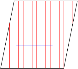
Figure 1. The torus $\omega_{T}$. A vertical segment of length $M$ (colored in red) intersects a horizontal slit (colored in blue) of length $|K|$.

Lemma 4.1.

For almost every $T$ we have that $\hat{\omega}$ is a limit point of $\{g_{t}\omega_{T}\}_{t\geq 0}.$

Proof.

Let $U^{+}$ denote the subgroup $\begin{pmatrix}1&\ast\\ 0&1\end{pmatrix}\ltimes\begin{pmatrix}\ast\\ 0\end{pmatrix}$ of $SL(2,{\mathbb{R}})\ltimes{\mathbb{R}}^{2}$. Then, $U^{+}$ is the expanding horospherical subgroup with respect to the action of $g_{t}$, or in other words, the orbits of $U^{+}$ are the unstable manifolds for the flow $g_{t}$.

By construction, map $T\to\omega_{T}$ projects to a positive measure subset ${\mathcal{D}}$ of a single $U^{+}$ orbit on ${\mathcal{M}}_{1,2}$. Moreover, the pushforward of the Lebesgue measure on the space of 3-IET’s to ${\mathcal{D}}$ is absolutely continuous with respect to the pushforward of the Haar measure on $U^{+}$ to ${\mathcal{D}}$. The lemma then follows from the ergodicity of $g_{t}$. ∎

Corollary 4.2.

For every $\delta>0$ and almost all $T$, there exists arbitrarily large $t>0$ with $g_{t}\omega_{T}\in B(\hat{\omega},\delta)\cap{\mathcal{S}}$.

Proof. Since $\hat{\omega}$ is square, for $p\in\hat{\omega}$, $F^{1}_{\hat{\omega}}p=p$. Therefore, for $\omega^{\prime}\in B(\hat{\omega},\delta^{\prime})$ and $p\in\omega^{\prime}$, $F^{1}_{\omega^{\prime}}p$ is within $c_{1}(\delta^{\prime})$ of $p$, where $c_{1}(\delta^{\prime})\to 0$ as $\delta^{\prime}\to 0$. Write $F^{1}_{\omega^{\prime}}p-p=(v_{1},v_{2})$, and note that for $\delta^{\prime}>0$ sufficiently small and for small $s\in{\mathbb{R}}$, for $p\in g_{s}\omega^{\prime}$, we have

$$F^{1}_{g_{s}\omega^{\prime}}p-p=(e^{-s}v_{1},1-e^{s}+e^{s}v_{2}).$$

Therefore, given $\omega^{\prime}\in B(\hat{\omega},\delta)$, we can choose $s\in{\mathbb{R}}$, with $|s|<c_{2}(\delta^{\prime})$ where $c_{2}(\delta^{\prime})\to 0$ as $\delta\to 0$, such that $1-e^{s}+e^{s}v_{2}=0$, i.e. $g_{s}\omega^{\prime}\in{\mathcal{S}}$. We have $g_{s}\omega^{\prime}\in B(\hat{\omega},c_{3}(\delta^{\prime}))$ with $c_{3}(\delta^{\prime})\to 0$ as $\delta^{\prime}\to 0$.

Suppose $T$ is such that $\hat{\omega}$ is a limit point of $\{g_{t}\omega_{T}\}_{t\geq 0}$. Choose $\delta^{\prime}>0$ such that $c_{3}(\delta^{\prime})<\delta$ and choose $t^{\prime}$ such that $g_{t^{\prime}}\omega_{T}\in B(\hat{\omega},\delta^{\prime})$ and then let $t=t^{\prime}+s$ where $s$ is as in the previous paragraph. Then $g_{t}\omega_{T}\in B(\hat{\omega},\delta)\cap{\mathcal{S}}$ as required. ∎

We now apply $g_{t}$ to Figure 1, with $t=\log M$. Note that $\psi_{M}(x)$ is also the intersection number between a vertical segment $\gamma_{1}$ of length $1$ and a horizonal slit $\gamma_{2}$ of length $M|K|$ (see Figure 2). From now on, we assume that $g_{t}\omega_{T}\in B(\hat{\omega},\delta)\cap{\mathcal{S}}$ for some $\delta\ll 1$.

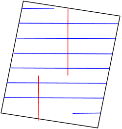
Figure 2. The torus $g_{\log M}\omega_{T}$: A vertical segment $\gamma_{1}$ of length $1$ (drawn in red) intersects a horizontal slit $\gamma_{2}$ of length $M|K|$ (drawn in blue). If we also assume that $g_{\log M}\omega_{T}\in B(\hat{\omega},\delta)\cap{\mathcal{S}}$ then the torus $g_{\log M}\omega_{T}$ is nearly square, and the two endpoints of $\gamma_{1}$ are on the same horizontal line segment, of length at most $1/2+O(\delta)$.

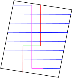
Figure 3. Closing the curves. We complete the vertical segment $\gamma_{1}$ to a closed curve $\hat{\gamma_{1}}$ by adding a horizontal segment $\zeta_{1}$ (drawn in green). Note that since $g_{t}\omega_{T}\in B(\hat{\omega},\delta)\cap{\mathcal{S}}$, the length of $\zeta_{1}$ is at most $1/2+O(\delta)$. Similarly, we close up the horizontal slit $\gamma_{2}$ to obtain a closed curve $\hat{\gamma}_{2}$ by adding in a horizontal segment $\zeta_{2}$ and a vertical segment $\zeta_{2}^{\prime}$ (drawn in purple).

The following lemma references Figure 3.

Lemma 4.3.

There exists $m$ so that if the green segment does not cross the purple segment then the number of times a trajectory of length 1 crosses $g_{t}K$ (the blue lines) is either $m$ or $m+1$. Moreover it is $m+1$ if it does not cross the (horizontal) purple segment and $m$ if it does.

In other words, for the set of points $x$ whose green segment does not cross the purple segment, ${\phi_{M}(x)}$ is $m$ if its red segment crosses the purple segment (where $\phi_{M}$ is as in (4.2)) and $\phi_{M}(x)=m+1$ if it does not.

Note that because Figure 3 is of $g_{\log(M)}\omega_{T}$, vertical trajectories of length 1 in Figure 3 correspond to vertical trajectories of length $M$ on $\omega_{T}$.

Proof.

Indeed, the family of curves we define are all homotopic and so their intersection with $\hat{\gamma}_{2}$ is all the same. So for such curves, if the green and purple segments have intersection number zero then the intersection of the red segment and blue segment depends only on the intersection of the purple segment and the red segment, which by construction is either 0 or 1. ∎

Lemma 4.4.

For all $\epsilon>0$ there exists $\delta>0$ so that if $\omega\in B(\hat{\omega},\delta)\cap\mathcal{S}$ and the flow $F^{s}_{\omega}$ is minimal then there exists $\rho<\epsilon$ and $L\in{\mathbb{N}}$ so that for any interval $J$ with $|J|=\rho$ we have

• $\lambda\left(\bigcup_{s\in[0,L)}F^{s}J\right)>1-\epsilon$

• For all $0\leq s<\ell<L$ we have $F^{s}J\cap F^{\ell}J=\emptyset$

• $F^{1}J$ is horizontally adjacent to $J$.

Proof.

Suppose $p$ is a point in $\omega$, and $\omega\in\mathcal{S}$. Then, $F^{1}p$ is horizontally adjacent to $p$. For all $\epsilon>0$ there exists $\delta>0$ so that if $\omega$ is in $\mathcal{S}\cap B(\hat{\omega},\delta)$ then $F^{1}p$ is translated by less than $\frac{\epsilon}{9}$. Since the vertical flow on $\omega$ is minimal, $F^{1}p\neq p$. Therefore, $F^{1}p$ is translated horizontally by some amount $\rho>0$. Let $J$ be a horizontal interval of length $\rho$. We choose $L=\min\{s>0:F^{s}J\cap J\neq\emptyset\}$. We have that $\lambda\left(\bigcup_{s\in[0,L)}F^{s}J\right)>1-\rho$. Indeed, $\bigcup_{s\in[0,L+1)}F^{s}J=\omega$. ∎

Proposition 4.5.

For any $a,b\in\mathbb{Z}$ and $\frac{c}{5}>\epsilon>0$ there exists $\delta>0$, $t_{0}>0$ so that if $g_{t}\omega_{T}\in B(\hat{\omega},\delta)\cap\mathcal{S}$, $\lambda(K)>c$ and $t>t_{0}$ then there exist

• $n\in\mathbb{Z}$, $r\in{\mathbb{N}},L\in\mathbb{N}$

• an interval $J\subset K$, and a measurable set $B\subset K$

so that the minimal return time (under $T$) to $J$ is at least $\frac{3}{2}r$, and for $A=\bigcup_{i=0}^{r}T^{i}J$ we have $\lambda(A)>\frac{1}{2}\lambda(K)-\epsilon,\lambda(B)>\frac{1}{2}\lambda(K)-\epsilon$ and the sets $A$ and $B$ satisfy

$$d(T^{n}x,T^{a}x)<\epsilon\text{ for all }x\in A$$

and

$$d(T^{n}x,T^{b}x)<\epsilon\text{ for all }x\in B.$$

Moreover, $T^{i}J\cap T^{j}J=\emptyset$ for all $0\leq i<j\leq\frac{3}{2}r$. Lastly, if $\nu^{(a)}$ is the joining supported on $\{(x,T^{a}x)\}$ then for all $x\in A$ we have

$$d_{KR}\left(\frac{1}{L}\sum_{i=0}^{L-1}\delta_{(T^{i}x,T^{i+n}x)},\nu^{(a)}\right)<2\epsilon$$

and if $\nu^{(b)}$ is the joining supported on $\{(x,T^{b}x)\}$ then for all $x\in B$ we have

$$d_{KR}\left(\frac{1}{L}\sum_{i=0}^{L-1}\delta_{(T^{i}x,T^{i+n}x)},\nu^{(b)}\right)<2\epsilon.$$

Remark 2.

Specializing to the case where $a=0$ and $b=k$, we see that $\frac{1}{2}(Id+T^{k})$ is in the weak closure of the powers of $T$. Veech showed that almost every 3-IET has simple spectrum [16, Theorem 1.3]. Combining these two facts with Ryzhikov’s [13, Theorem 6.1 (3) and (4)] we have that the spectrum of $T^{n}$ and $\underbrace{T\times...\times T}_{n\text{ times}}$ are simple for all $n>0$.

Proof.

In view of Lemma 4.4, we can choose $\delta$ so small that for any $\omega\in B(\hat{\omega},\delta)$,

1. The horizontal purple line has length between $\frac{1}{2}-\frac{\epsilon}{4}$ and $\frac{1}{2}+\frac{\epsilon}{4}$.

2. $F^{1}_{\omega}x=\begin{pmatrix}1&0\\ 0&1\end{pmatrix}\ltimes\begin{pmatrix}\rho\\ 0\end{pmatrix}x$ where $0<\rho\leq\frac{\epsilon}{10(|a|+|b|)}$.

Because $T\times T$ is uniquely ergodic on the support of $\nu^{(a)}$ and $\nu^{(b)}$ there exists $L_{0}$ so that if $d(p_{i},T^{a+i}y)<\epsilon$ for all $0\leq i\leq L$ then

(4.3) $$d_{KR}\left(\frac{1}{L}\sum_{i=0}^{L-1}\delta_{(T^{i}y,p_{i})},\nu^{(a)}\right)<2\epsilon,\qquad d_{KR}\left(\frac{1}{L}\sum_{i=0}^{L-1}\delta_{(T^{i}y,p_{i})},\nu^{(b)}\right)<2\epsilon$$

for all $L\geq L_{0}$ and $y\in K$. Indeed, $T\times T$ is uniquely ergodic on $\text{supp}(\nu^{(a)})$ and $\text{supp}(\nu^{(b)})$ and uniquely ergodic systems have uniform convergence of Birkhoff averages of continuous functions (see for example [3, Proposition 4.7.1]). We choose $t_{0}$ so large that any vertical trajectory of length $e^{t_{0}}$ on $\omega_{T}$ crosses $K$ at least $L_{0}$ times. We further assume $L_{0}>\max\{|a|,|b|\}$.

We now set about defining $J$ and $A$. Let $V$ be the horizontal purple line segment. Let $\rho$ be as in the previous lemma for $g_{t}\omega_{T}$. For any horizontal interval $I$ on $g_{t}\omega_{T}$ of length $\rho$ we have one of the following mutually exclusive possibilities:

1. $\bigcup_{s\in[0,1)}F^{s}(I)\cap V=\emptyset$

2. There exists $s\in[0,1)$ so that $F^{s}(I)\subset V$.

3. $\bigcup_{s\in[0,1)}F^{s}(I)\cap(\partial V)\neq\emptyset$

Note that by Lemma 4.3 there exists $m$ so that if $I\subset K$ so that if (b) holds then $\phi_{M}(x)=m$ and similarly if $I\subset K$ so that (a) holds then $\phi_{M}(x)=m+1$.

Let $\hat{A}$ be the set of points in $g_{t}\omega_{T}$ which belong to some horizontal interval of length $\rho$ satisfying (b). Let

(4.4) $$\tilde{A}=\bigcap\limits_{s\in[-2-|a-b|,2+|a-b|]}F^{s}_{g_{t}\omega_{T}}\hat{A}.$$

Let $\rho>0$ be given by Lemma 4.4 and $I$ be an interval of length $\rho$ in $\tilde{A}\cap g_{t}K$ so that $F^{-1}I\not\subset\tilde{A}$. Now $F^{1}I$ is horizontally adjacent to $I$, and so $F^{j}I$ is horizontally $j\rho$ over from $I$. So by our assumption on the length of $I$, we have

(4.5) $$F^{j}I\subset\tilde{A},\quad\text{ for all }\quad 0\leq j\leq\frac{|V|}{\rho}-2(2+|a+b|)-3\equiv\hat{p}.$$

(Note that by (ii) and the fact that $|V|>\frac{1}{2}-\epsilon$ we have $\hat{p}\geq 1$.)

We now use what we have done for the flow on $g_{t}\omega_{T}$ to establish some of our claims about the IET, $T$. Let $r$ be the cardinality of the set of intervals of length $\rho$ in $\bigcup_{s\in[0,\hat{p})}F^{s}I\cap K$. Note that because in our set $\hat{A}$ a vertical trajectory of length 1 crosses $g_{t}K\subset g_{t}\omega_{T}$ exactly $m$ times, $r=m\hat{p}$.

Let $A^{\prime}=g_{-t}\hat{A}\cap K\subset\omega_{T}\cap K$, which we can consider as a subset of the domain of $T$ as well (because it is contained in $K$). Note that we have

(4.6) $$\phi_{e^{t}}(x)=m\qquad\text{for $x\in A^{\prime}$.}$$

We also have for all $x\in A^{\prime}$,

(4.7) $$d(F^{e^{t}}x,x)=e^{-t}\rho,$$

because when we apply $g_{-t}$ to pull back our dynamics from $g_{t}\omega_{T}$ back to $\omega_{T}$ we contract horizontal distances by $e^{-t}$. It follows from (4.2), (4.6) and (4.7) that

(4.8) $$d(T^{m}(x),x)=e^{-t}\rho\qquad\text{for all $x\in A^{\prime}$.}$$

Let $J$ denote the interval corresponding to $I$ in the domain of our IET, $T$. That is, we consider $J=g_{-t}I\subset K\subset\omega_{T}$, which since it is in $K$ we consider as an interval in the domain of $T$. Let $A=\bigcup_{i=0}^{r-1}T^{i}J$, which we can consider as a subset of $K\subset\omega_{T}$. We now claim that

(4.9) $$A\subset g_{-t}\tilde{A}\cap K.$$

Indeed, by (4.5), we have

(4.10) $$F^{se^{t}}J\subset g_{-t}\tilde{A}\qquad\text{for all $0\leq s\leq\hat{p}$.}$$

It follows in view of (4.6), that for $x\in J$,

(4.11) $$\phi_{\hat{p}e^{t}}(x)=\sum_{k=0}^{\hat{p}-1}\phi_{e^{t}}(F^{ke^{t}}x)=m\hat{p}=r.$$

By (4.2), we have for $x\in J$ and $i\in{\mathbb{N}}$,

$$T^{i}x=F^{s}x,\quad\text{where $s$ is such that $\phi_{s}(x)=i$. }$$

Since for a fixed $x\in J$, the map $s\to\phi_{s}(x)$ is monotone increasing in $s$, for $0<i<r$ we have in view of (4.11),

$$T^{i}x=F^{s}x\quad\text{where $s<\hat{p}$.}$$

This, together with (4.10) implies (4.9). The same argument shows that

(4.12) $$T^{\ell}x\in A^{\prime}\qquad\text{for $x\in A$ and $|\ell|\leq m(|a-b|+1)$.}$$

We now claim that for all $x\in A$ we have:

$$d(T^{n}x,T^{a}x)\leq d(T^{a}x,T^{a}x)+\sum_{i=1}^{|a-b|}d(T^{im+a}x,T^{(i-1)m+a}x)\leq\epsilon e^{-t}\leq\epsilon.$$

Indeed, by (4.12) and (4.8) we have $d(T^{jm+a}x,T^{(j-1)m+a}x)=\rho e^{-t}$ for all $|j|\leq|a-b|$, because $|a|<m$. We obtain the second inequality by (ii).

We now show that for all $x\in A$

$$d_{KR}(\frac{1}{m}\sum_{i=0}^{m-1}\delta_{(T^{i}x,T^{i+n}x)},\nu^{(a)})<2\epsilon.$$

By construction, if $x\in A$ then $T^{i}x\in A^{\prime}$ for all $-m\leq i\leq m$. So we have that $d(T^{i+n}x,T^{i+a}x)<\epsilon$ for all $|i|\leq|m|$. So by (4.3) and the fact that $m\geq L_{0}$ we have our condition on $d_{KR}$.

We now show that $\lambda(A)>\frac{1}{2}\lambda(K)-\epsilon$. This follows from the fact that by (ii) the measure of the set of $x\in g_{t}\omega_{T}$ so that $F^{\ell}x$ crosses the horizontal purple strip for $0\leq\ell\leq 1$ and $-1\leq\ell\leq 0$ and $F^{s}_{g_{t}\omega_{T}}x$ does not have this property for some $-1\leq s\leq 1$ has measure at most $2\frac{\epsilon}{10(|a|+|b|)}$. By our condition on the length of the purple horizontal strip, the measure condition on $A$ is completed.

The fact that the return time of $T$ to $J$ is at most $\frac{3}{2}r$ follows from the fact that the measure of $A^{c}$ is at most $\frac{1}{2}\lambda(K)+\epsilon$ and so the orbit of $J$ after leaving $A$ and before returning to $J$ has measure at least $\frac{1}{2}\lambda(K)-\epsilon-\epsilon>\frac{1}{2}\lambda(A)$. So $J$ has at least $\frac{1}{2}r$ images outside of $A$ before part of it returns.

We now similarly define $B\subset A^{c}$ with the desired properties. First let

$$\hat{B}=\{x\in g_{t}\omega_{T}:\cup_{s\in[-3-|a-b|,3+|a-b|]}F^{s}_{g_{t}\omega_{T}}(x)\cap V=\emptyset\}.$$

Similarly to before let $\tilde{B}=\cap_{s\in[-1,1]}F^{s}_{g_{t}\omega_{T}}\hat{B}$ and $B=g_{-t}\tilde{B}\cap K\subset\omega_{T}$, considered as a subset of the domain of $T$. Now as above, by Lemma 4.3 if $x\in\tilde{B}$ then we have that a vertical trajectory of length 1 or -1 emanating from $x$ crosses $g_{t}K$ exactly $m+1$ times. Moreover, $F^{s}_{g_{t}\omega_{T}}x$ has this property for all $-|a-b|\leq s\leq|a-b|$. Since $n=b+(m+1)(a-b)$, for any $x\in B$ and $|i|\leq m$ we have $d(T^{n}T^{i}x,T^{b}T^{i}x)\leq\sum_{i=1}^{|a-b|}d(T^{i(m+1)}x,T^{(i-1)(m+1)}x)\leq\epsilon$. Thus, as above we have $d_{KR}(\frac{1}{m}\sum_{i=0}^{m-1}\delta_{(T^{i}x,T^{i+n}x)},\nu^{(b)})<2\epsilon$ for all $x\in B$. The fact that $\lambda(B)>\lambda(K)-\epsilon$ is similar to the case of $\lambda(A)$ above.

∎

Now given two number $a,b$ we may iteratively apply Proposition 4.5 to obtain the assumptions of Proposition 3.1. Indeed, we choose $\epsilon_{i}$ satisfying assumptions (c) and (e). We apply Proposition 4.5 to the pair of numbers $(a,b)$ and $\epsilon=\epsilon_{1}$ to obtain $m$, $A,B$ and $r$. Denote $m$ by $a_{1}$. We apply Proposition 4.5 to the pair of numbers $(a,b)$ and $\epsilon=\epsilon_{1}$ to obtain $m$, $r^{\prime}$, $A^{\prime},B^{\prime}$, and denote $m$ by $b_{1}$. We repeat this procedure with $a_{1}$ and $b_{1}$ in the place of $a$ and $b$ and $\epsilon_{2}$ in place of $\epsilon$ and obtain $a_{2},b_{2}$. We further request that the interval $J$ produced by Proposition 4.5 have $\max\{r,r^{\prime}\}\lambda(J)<\epsilon_{2}$. Iterating this we have the conditions of Proposition.

Proof of Theorem 1.1.

Let $\mu$ be an invariant measure for $T\times T$. By Corollary 2.3 there exists $n_{1},...,n_{d}$ so that $\nu_{i}$ is the joining supported on $\{(x,T^{n_{i}}x)\}$ and $d_{KR}(\mu,\frac{1}{d}\sum_{i=1}^{d}\nu_{i})<\epsilon$. For each pair $n_{i},n_{i+1}$ and $\frac{\epsilon}{2}$ we apply Proposition 4.5 to obtain $\delta$, $t_{0}$. We further do this for the pair $n_{d},\,n_{1}$. We choose $\delta$ to be the smallest of these and $t_{0}$ to be the largest. We obtain $t>t_{0}$ so that $g_{t}\omega_{T}\in B(\hat{\omega},\delta)$. We then obtain $m_{i}$, $r_{i}$ which we denote $n_{i}^{(1)}$ and $r_{i}^{(1)}$. We now repeat this $n_{i}^{(1)}$ in place of $n_{i}$, $\frac{\epsilon}{2^{2}}$ in place of $\frac{\epsilon}{2}$ and $\max\{r_{i}^{(1)}\}$. In doing this we obtain $n_{i}^{(2)}$ and $r_{i}^{(2)}$. We repeat this recursively having our $k$th choice of $\epsilon$ be $\frac{\epsilon}{2^{k}}$.

We are now left to prove that there is an ergodic self-joining that is neither $\lambda\times\lambda$ nor one-to-one on almost every fiber. Let $\nu_{0}^{(1)}$ be the self-joining carried on $\{(x,x)\}$ and $\nu_{0}^{(2)}$ be the self-joining carried on $\{(x,Tx)\}$. Let $\epsilon_{i}>0$ satisfy that

(4.13) $$d(x,Tx)>40C\sum_{i=1}^{\infty}\epsilon_{i}$$

and

(4.14) $$d_{KR}(\lambda\times\lambda,\frac{1}{2}(\nu_{0}^{(1)}+\nu_{0}^{(2)}))>4C\sum_{i=1}^{\infty}\epsilon_{i},$$

where $C$ is as in the conclusion of Proposition 3.1. We apply Proposition 3.1 for these $\epsilon_{i}$ as above to obtain $\nu_{i}^{(1)},\nu_{i}^{(2)}$ and their weak-* limit $\nu_{\infty}$, an ergodic measure which by (4.14) is not $\lambda\times\lambda$. The following lemma show $\nu_{\infty}$ can not be one-to-one on almost every fiber.

Lemma 4.6.

If $\mu$ is a measure that is one-to-one on almost every fiber then $\mu$ can not be the weak-* limit of a sequence of measures $\tilde{\nu}_{i}$ that are two-to-one on almost every fiber and so that

$$\lambda(\{x:diam(supp(\tilde{\nu}_{i})_{x})>\delta\})>\frac{3}{4}$$

for infinitely many $i$.

Proof.

There exists $f:[0,1)\to[0,1)$ measurable so that $\mu$ is carried on $\{(x,f(x))\}$. By Lusin’s Theorem there exists $\mathcal{K}$ compact with $\lambda(\mathcal{K})>\frac{99}{100}$ so that $f|_{\mathcal{K}}$ is uniformly continuous. Let $s>0$ be so that $d(f(x),f(y))<\frac{\delta}{8}$ for all $x,y\in\mathcal{K}$ with $d(x,y)<s$. Choose an interval $I$ with $|I|\leq s$, $\lambda(I\cap\mathcal{K})>\frac{99}{100}\lambda(I)$ and

(4.15) $$\lambda(\{x\in I:diam((\tilde{\nu}_{i})_{x})>\delta\})>\frac{1}{2}$$

for infinitely many $i$. Let $p=f(x)$ for some $x\in I\cap\mathcal{K}$ and let $g:[0,1)\times[0,1)\to\mathbb{R}$ be a 1-Lipschitz function so that

• $g|_{I^{c}\times[0,1)}\equiv 0$

• $g|_{I\times B(p,\frac{\delta}{4})}\equiv 0$

• $g(x,y)=\min\{d(x,\partial I),d(y,\partial B(p,\frac{\delta}{4})),\frac{\delta}{4}\}$ for all $(x,y)\in I\times(B(p,\frac{\delta}{4}))^{c}$.

Now $\int gd\sigma\leq.01|I|\cdot\|g\|_{\sup}\leq.01|I|\cdot\min\{\frac{\delta}{4},\frac{|I|}{2}\}$. On the other hand if $\tilde{\nu}_{i}$ satisfies (4.15) then on a set of $x\in I$ of measure at least $\frac{|I|}{3}$ we have one of the two points in $(\tilde{\nu}_{i})_{x}$ is at least $\frac{\delta}{2}$ away from $p$. A subset of these $x$ of measure at least $\frac{|I|}{6}$ satisfies $d(x,\partial I)\geq\frac{1}{12}|I|$. So $\int gd\tilde{\nu}_{i}\geq\frac{|I|}{6}\min\{\frac{\delta}{4},\frac{|I|}{12}\}$. Since $g$ is 1-Lipschitz it follows that $d_{KR}(\mu,\tilde{\nu}_{i})>|I|\min\{|I|(\frac{1}{72}-\frac{1}{200}),\frac{\delta}{24}-\frac{\delta}{400}\}$ proving the lemma. ∎

Letting $\tilde{\nu}_{i}=\frac{1}{2}(\nu_{i}^{(1)}+\nu_{i}^{(2)})$ and seeing that by (4.13) they satisfy the condition in the lemma, we see $T$ is not 2-simple. ∎

References

- [1] Ageev, O. N. A typical dynamical system is not simple or semisimple. Ergodic Theory Dynam. Systems 23 (2003), no. 6, 1625–1636
- [2] Boshernitzan, M. A unique ergodicity of minimal symbolic flows with linear block growth. J. Analyse Math. 44 (1984/85), 77–96.
- [3] Brin, M; Stuck, G Introduction to dynamical systems. Cambridge University Press, Cambridge, 2002. xii+240 pp.
- [4] Fogg, N. Pytheas Substitutions in dynamics, arithmetics and combinatorics. Edited by V. Berth , S. Ferenczi, C. Mauduit and A. Siegel. Lecture Notes in Mathematics, 1794. Springer-Verlag, Berlin, 2002. xviii+402 pp.
- [5] Janvresse, É; de la Rue, T; Ryzhikov, V Around King’s rank-one theorems: flows and ?n-actions. Dynamical systems and group actions. 143–161, Contemp. Math., 567, Amer. Math. Soc., Providence, RI, 2012.
- [6] Katok, A. B.; Stepin, A. M. Approximations in ergodic theory. Uspehi Mat. Nauk 22 1967 no. 5 (137), 81–106.
- [7] Khinchin, A. Continued fractions. With a preface by B. V. Gnedenko. Translated from the third (1961) Russian edition. Reprint of the 1964 translation. Dover Publications, Inc., Mineola, NY, 1997. xii+95 pp.
- [8] King, J. The commutant is the weak closure of the powers, for rank-1 transformations, Ergodic Theory Dynam. Systems 6 (1986), no. 3, 363–384.
- [9] King, J. Flat stacks, joining closure and genericity. Preprint
- [10] Lindenstrauss, J.; Olsen, G.; Sternfeld, Y. The Poulsen simplex, Ann. Inst. Fourier (Grenoble) 28 (1978), no. 1, vi, 91–114.
- [11] Rudolph, D. An example of a measure preserving map with minimal self-joinings, and applications. J. Analyse Math. 35 (1979), 97–122
- [12] Ryzhikov, V. V. Mixing rank and minimal self-joining of actions with an invariant measure. Mat. Sb. 183 (1992), no. 3, 133–160.
- [13] Ryzhikov, V. V. Weak limits of powers, the simple spectrum of symmetric products, and mixing constructions of rank 1. Mat. Sb. 198 (2007), no. 5, 137–159; translation in Sb. Math. 198 (2007), no. 5-6, 733–754
- [14] Ryzhikov, V. V. Self-joinings of rank-one actions and applications. École de Théorie Ergodique, 193–206, Sémin. Congr., 20, Soc. Math. France, Paris, 2010.
- [15] Veech, W. A. A criterion for a process to be prime, Monatsh. Math. 94 (1982), no. 4, 335–341.
- [16] Veech, W. A. The metric theory of interval exchange transformations. I. Generic spectral properties, Amer. J. Math. 106 (1984), no. 6, 1331–1359.