$\ell$-Boson stars

Abstract

We present new, fully nonlinear numerical solutions to the static, spherically symmetric Einstein-Klein-Gordon system for a collection of an arbitrary odd number $N$ of complex scalar fields with an internal $U(N)$ symmetry and no self-interactions. These solutions, which we dub $\ell$-boson stars, are parametrized by an angular momentum number $\ell=(N-1)/2$, an excitation number $n$, and a continuous parameter representing the amplitude of the fields. They are regular at every point and possess a finite total mass. For $\ell=0$ the standard spherically symmetric boson stars are recovered. We determine their generalizations for $\ell>0$, and show that they give rise to a large class of new static configurations which might have a much larger compactness ratio than $\ell=0$ stars.

I Introduction

Boson stars composed of massive scalar fields are among the most promising exotic objects that may populate the universe. They were originally proposed by Kaup Kaup68 and Ruffini and Bonazzola Ruffini:1969qy in the late sixties, and explored in more detail during the subsequent decades in e.g. Refs. Colpi:1986ye ; Friedberg87 ; Gleiser:1988rq ; Lee:1988av ; Seidel:1990 ; Guzman:2004wj (see also Jetzer:1991jr ; Lee:1991ax ; Schunck:2003kk ; Liebling:2012fv for reviews). Even though they remain hypothetical, boson stars are frequently considered as candidates for black hole mimickers Torres:2000dw ; Guzman:2005bs ; AmaroSeoane:2010qx , massive compact objects made of axions Hogan:1988mp ; Kolb:1993zz ; Barranco:2010ib , or even the core of the galactic halos Sin:1992bg ; Schive:2014dra in the context of fuzzy dark matter Marsh:2015xka ; Hui:2016ltb .

It is within this line that we present a new class of static solutions to the Einstein-Klein-Gordon (EKG) system which generalize the known boson stars by considering a collection of an arbitrary odd number $N$ of free complex scalar fields of the same mass. For $N=1$ these configurations reduce to the standard, spherically symmetric boson star configurations. For $N>1$, new static configurations are obtained which are still spherically symmetric if the collection of scalar fields are excited in an appropriate way.

Our approach is to consider that spacetime curvature is sourced by a collection of classical fields that compound a spherically symmetric configuration. The construction is based on a method introduced in Ref. Olabarrieta:2007di , where it was shown that for the case in which the fields are real and massless, and as long as all the harmonics with given angular momentum number $\ell=(N-1)/2$ are excited with equal amplitude, the total stress energy-momentum tensor is spherically symmetric. In this way, it is possible to study the dynamics of scalar fields which, individually, have angular momentum, while keeping the spherical symmetry of the spacetime. As remarked in Olabarrieta:2007di this resembles a spherically symmetric kinetic gas where the individual particles may rotate but the configuration is spherical. The authors of Ref. Olabarrieta:2007di used this technique to study a possible effect of the angular momentum on the critical collapse of scalar field configurations.

In the present work we show that their method still works for a collection of complex, non-interacting massive scalar fields. The situation is similar to that in standard boson stars, where an internal $U(1)$ symmetry “hides” the time dependency of the field avoiding Derrick’s theorem Derrick:1964ww ; Diez-Tejedor:2013sza . If we extend the group of symmetry to higher values of $N$, then not only the time evolution, but also the angular dependency of the non-trivial harmonics with angular momentum number $\ell=(N-1)/2$ can be accommodated in the internal field space, leading to new static and spherically symmetric solutions to the EKG system. We refer to these objects as $\ell$-boson stars in this paper. The main goal of this work is to determine their domain of existence and to compare their properties with the standard $\ell=0$ boson stars.

The remainder of this article is organized as follows. In Sec. II we derive the spherically symmetric field equations for the particular collection of scalar fields belonging to a fixed angular momentum number $\ell$. Next, in Sec. III we demonstrate the local existence of solutions to the EKG system in the vicinity of the center. Based on a shooting algorithm starting from the local solution at the center, in Sec. IV we numerically solve the field equations to find the globally regular solutions describing the $\ell$-boson stars, and discuss their behavior, including their density profile and mass curves for different values of $\ell$. Conclusions and an outlook to future work are drawn in Sec. V, and relevant identities involving spherical harmonics that are needed in this article are derived in the Appendix at the end of the paper.

We use the signature $(-,+,+,+)$ for the spacetime metric, and natural units such that $\hbar=c=1$. The numerical solutions presented below are in Planck units, where we have also taken the gravitational constant equal to 1, $G=1$.

II Field equations

In this section, we present the spherically symmetric EKG system that describes a collection of an arbitrary odd number of complex, non-interacting scalar fields $\Phi_{i}$, $i=1,\ldots,N$, of mass $\mu$ each, which are excited in an appropriate way consistent with the spacetime symmetries.

The stress energy-momentum tensor associated with such a collection of scalar fields is

$$T_{\mu\nu}=\frac{1}{2}\sum_{i}\left[\nabla_{\mu}\Phi_{i}^{*}\nabla_{\nu}\Phi_{i}+\nabla_{\mu}\Phi_{i}\nabla_{\nu}\Phi_{i}^{*}\right.$$

$$\left.-g_{\mu\nu}\left(\nabla_{\alpha}\Phi_{i}^{*}\nabla^{\alpha}\Phi_{i}+\mu^{2}\Phi_{i}^{*}\Phi_{i}\right)\right].$$ (1)

Here $\Phi_{i}^{*}$ denotes the complex conjugate of the field component $\Phi_{i}$, and $\nabla_{\mu}$ is the covariant derivative with respect to the spacetime metric $g_{\mu\nu}$. Notice that since the mass is the same for the $N$ fields, and they do not interact between themselves, this expression is invariant under $U(N)$ transformations in the internal field space. We assume that the different fields in the configuration satisfy the Klein-Gordon equation individually, such that $(\nabla_{\mu}\nabla^{\mu}-\mu^{2})\Phi_{i}=0$.

Following Olabarrieta:2007di we now consider solutions of the form

$$\Phi_{\ell m}(t,r,\vartheta,\varphi)=\phi_{\ell}(t,r)Y^{\ell m}(\vartheta,\varphi),$$ (2)

where the angular momentum number $\ell=(N-1)/2$ is fixed in the configuration and $m$, which plays the role of the index $i$ in Eq. (II), takes values $m=-\ell,-\ell+1,\ldots,\ell$. As usual $Y^{\ell m}$ denotes the standard spherical harmonics, and the amplitudes $\phi_{\ell}(t,r)$ are the same for all $m$. As shown in the Appendix this leads to a total stress energy-momentum tensor which is spherically symmetric. (The authors of Ref. Olabarrieta:2007di show a similar result valid for a collection of scalar fields which are, however, real and massless; for this reason we include here an independent proof.)

Representing the spacetime metric in terms of the Misner-Sharp mass $M(t,r)$ and the lapse function $\alpha(t,r)$, the line element is written as

$$ds^{2}=-\alpha^{2}dt^{2}+\gamma^{2}dr^{2}+r^{2}d\Omega^{2},\quad\gamma^{2}:=\frac{1}{1-\frac{2M}{r}},$$ (3)

with $r$ the areal radial coordinate and $d\Omega^{2}$ the standard line element on the unit two-sphere. With this notation and the assumption in Eq. (2), the EKG system yields

$$\dot{M} = -\frac{\kappa_{\ell}r^{2}}{2}\frac{\alpha}{\gamma}j^{(\ell)},$$ (4a)

$$M^{\prime} = \frac{\kappa_{\ell}r^{2}}{2}\rho^{(\ell)},$$ (4b)

$$\frac{\alpha^{\prime}}{\alpha} = \gamma^{2}\left(\frac{M}{r^{2}}+\frac{\kappa_{\ell}r}{2}S^{(\ell)}\right),$$ (4c)

$$\dot{\phi}_{\ell} = \alpha\Pi_{\ell},$$ (4d)

$$\dot{\Pi}_{\ell} = \frac{1}{r^{2}\gamma}\left(r^{2}\frac{\alpha}{\gamma}\phi_{\ell}^{\prime}\right)^{\prime}+\frac{\kappa_{\ell}r}{2}\alpha\gamma j^{(\ell)}\Pi_{\ell}$$ (4e)

$$- \alpha\left(\mu^{2}+\frac{\ell(\ell+1)}{r^{2}}\right)\phi_{\ell},$$

where $\kappa_{\ell}:=(2\ell+1)\>G$ is the (rescaled) gravitational coupling constant and where the source terms are given by

$$\rho^{(\ell)} = |\Pi_{\ell}|^{2}+|\chi_{\ell}|^{2}+\left(\mu^{2}+\frac{\ell(\ell+1)}{r^{2}}\right)|\phi_{\ell}|^{2},$$ (5a)

$$S^{(\ell)} = |\Pi_{\ell}|^{2}+|\chi_{\ell}|^{2}-\left(\mu^{2}+\frac{\ell(\ell+1)}{r^{2}}\right)|\phi_{\ell}|^{2},$$ (5b)

$$j^{(\ell)} = -2\mbox{Re}(\Pi_{\ell}^{*}\chi_{\ell}).$$ (5c)

Here $\Pi_{\ell}:=\alpha^{-1}\dot{\phi}_{\ell}$ is the conjugate momentum associated with the scalar field, $\chi_{\ell}:=\gamma^{-1}\phi_{\ell}^{\prime}$, and a dot and a prime denote partial derivatives with respect to $t$ and $r$, respectively.

In the following, we look for solutions with a harmonic time-dependency,

$$\phi_{\ell}(t,r)=e^{i\omega t}\psi_{\ell}(r),$$ (6)

with some real frequency $\omega$ (taken to be positive without loss of generality) and a real-valued function $\psi_{\ell}(r)$. This provides a nonlinear eigenvalue problem for the quantities $(M,\alpha\gamma,\psi_{\ell})$ which can be written as

$$M^{\prime}=\frac{\kappa_{\ell}r^{2}}{2}\left[\frac{\psi_{\ell}^{\prime 2}}{\gamma^{2}}+\left(\mu^{2}+\frac{\omega^{2}}{\alpha^{2}}+\frac{\ell(\ell+1)}{r^{2}}\right)\psi_{\ell}^{2}\right],\quad$$ (7a)

$$\frac{(\alpha\gamma)^{\prime}}{\alpha\gamma^{3}}=\kappa_{\ell}r\left[\frac{\psi_{\ell}^{\prime 2}}{\gamma^{2}}+\frac{\omega^{2}}{\alpha^{2}}\psi_{\ell}^{2}\right],$$ (7b)

$$\frac{1}{r^{2}\alpha\gamma}\left(\frac{r^{2}\alpha}{\gamma}\psi_{\ell}^{\prime}\right)^{\prime}=\left(\mu^{2}-\frac{\omega^{2}}{\alpha^{2}}+\frac{\ell(\ell+1)}{r^{2}}\right)\psi_{\ell}.$$ (7c)

For the particular case of $N=1$, i.e. $\ell=0$, these equations reduce to the ones describing static boson stars with a zero angular momentum scalar field. These configurations have been studied extensively in the literature, and may be parametrized by the central value of the field and an excitation number Jetzer:1991jr ; Lee:1991ax ; Schunck:2003kk ; Liebling:2012fv .

In the following, we study the solutions for $N>1$, i.e. $\ell>0$. In this case the presence of the centrifugal term $\ell(\ell+1)/r^{2}$ in the EKG system requires $\psi_{\ell}$ to vanish at the center of the configuration and to decay with a specific rate as $r\to 0$. This is analyzed next.

III Local solutions near the center

For $\ell=0$, a full proof for the existence of regular solutions of finite mass was given by Bizoń and Wasserman in Ref. Bizon:2000es . Although it would be very interesting to generalize their results to arbitrary values of $\ell$, a full existence proof clearly lies beyond the scope of this work. However, for the purpose of this paper we found it useful to generalize one partial result given in Bizon:2000es (see Proposition 3.1 of that paper), regarding the local existence of solutions near the center. This provides a rigorous discussion for the existence and behavior of the solutions in the vicinity of $r=0$, and allows us to set up the correct boundary conditions to start the numerical integration scheme described in the next section.

In order to discuss the solutions in the vicinity of $r=0$, it is convenient to introduce the following dimensionless quantities:

$$x:=\mu r, \;f(x):=\sqrt{\kappa_{\ell}}\psi_{\ell}(r),$$ (8a)

$$B(x):=2\mu M(r)/x^{2}, \;Q(x):=\frac{\mu}{\omega}\alpha(r)\gamma(r),$$ (8b)

in terms of which the system (7) can be rewritten as

$$\frac{d}{dx}(x^{2}B)=x^{2}\left[\frac{f_{x}^{2}}{\gamma^{2}}+\left(1+\frac{\gamma^{2}}{Q^{2}}+\frac{\ell(\ell+1)}{x^{2}}\right)f^{2}\right],\qquad$$ (9a)

$$\frac{d}{dx}\log Q=x\left[f_{x}^{2}+\frac{\gamma^{4}}{Q^{2}}f^{2}\right],$$ (9b)

$$\frac{1}{x^{2}Q}\frac{d}{dx}\left(\frac{x^{2}Q}{\gamma^{2}}f_{x}\right)=\left(1-\frac{\gamma^{2}}{Q^{2}}+\frac{\ell(\ell+1)}{x^{2}}\right)f.$$ (9c)

Here we have used the shorthand notation $f_{x}=df/dx$, and it is understood that $\gamma^{2}$ should be substituted by $[1-xB(x)]^{-1}$.

For $\ell=0$, it was shown in Ref. Bizon:2000es that for each positive values of $Q_{0}$ and $a_{0}$, there exists a local solution of the form

$$B(x) = {\cal O}(x),$$ (10a)

$$Q(x) = Q_{0}+{\cal O}(x^{2}),$$ (10b)

$$f(x) = a_{0}+{\cal O}(x^{2}),$$ (10c)

near the center $x=0$. In the following, we generalize this local existence result to arbitrary values of $\ell$. As mentioned above, the presence of the centrifugal term $\ell(\ell+1)/x^{2}$ drastically modifies the behavior of the fields close to the center. In fact, a heuristic approximation assuming $B\to 0$, $Q\to\textrm{const.}$ gives

$$-\frac{d}{dx}(x^{2}f_{x})+\ell(\ell+1)f\simeq 0,$$ (11)

which has solutions of the form $f\sim x^{\ell}$ or $f\sim x^{-\ell-1}$. Since we require regularity a the center, we discard the second possibility. We now show the existence of a two-parameter family of solutions for which

$$B(x) = {\cal O}(x^{2\ell-1}),$$ (12a)

$$Q(x) = Q_{0}\left[1+{\cal O}(x^{2\ell})\right],$$ (12b)

$$f(x) = \frac{a_{0}}{2\ell+1}x^{\ell}\left[1+{\cal O}(x^{2})\right].$$ (12c)

This implies $\alpha=\alpha_{c}[1+{\cal O}(x^{2\ell})]$, with $\alpha_{c}=Q_{0}\omega/\mu$, and $M={\cal O}(x^{2\ell+1})$, in terms of the original variables. Notice that these expressions are only valid as long as $\ell>0$.

In order to prove the existence of such solutions, we replace $f$ and its first derivative with the new fields $(G,H)$, such that

$$\left(\begin{array}[]{r}f(x)\\ xf_{x}(x)\end{array}\right)=\frac{x^{\ell}}{2\ell+1}\left(\begin{array}[]{cc}1&1\\ \ell&-(\ell+1)\end{array}\right)\left(\begin{array}[]{r}G(x)\\ H(x)\end{array}\right).$$ (13)

Note that (up to a constant $2\ell+1$) the two asymptotic solutions $f(x)=x^{\ell}$ and $f(x)=x^{-\ell-1}$ correspond to the fields $(G,H)=(1,0)$ and $(G,H)=x^{-2\ell-1}(0,1)$, respectively. In terms of the fields $u:=(B,Q,G,H)$, the system (9) can be rewritten in first-order form:

$$\frac{d}{dx}(x^{2}B) = x^{2\ell}F_{B}(x,u),$$ (14a)

$$\frac{dQ}{dx} = x^{2\ell-1}F_{Q}(x,u),$$ (14b)

$$\frac{dG}{dx} = F_{G}(x,u),$$ (14c)

$$\frac{d}{dx}(x^{2\ell+1}H) = -x^{2\ell+1}F_{G}(x,u),$$ (14d)

with the source terms given by

$$F_{B} = \frac{(x^{1-\ell}f_{x})^{2}}{\gamma^{2}}+\left[x^{2}\left(1+\frac{\gamma^{2}}{Q^{2}}\right)+\ell(\ell+1)\right](x^{-\ell}f)^{2},$$

$$F_{Q} = Q(x^{1-\ell}f_{x})^{2}+\frac{\gamma^{4}}{Q}x^{2}(x^{-\ell}f)^{2},$$ (15)

$$F_{G} = \gamma^{2}\left\{\left[x\left(1-\frac{\gamma^{2}}{Q^{2}}\right)+\ell(\ell+1)B\right](x^{-\ell}f)\right.$$

$$+\left[x^{2\ell-1}\left(x^{2}+\ell(\ell+1)\right)(x^{-\ell}f)^{2}-B\right](x^{1-\ell}f_{x})\Big{\}}.$$

In these expressions, $\gamma^{2}$ should be replaced with $[1-xB]^{-1}$ and the terms $x^{-\ell}f$ and $x^{1-\ell}f_{x}$ should be rewritten in terms of $G$ and $H$ according to Eq. (13). Note that when rewritten in this way, these terms are regular at $x=0$, which implies that the source terms $F_{B}$, $F_{Q}$ and $F_{G}$ are regular as well at $x=0$ for all $\ell\geq 1$.

Eqs. (14) can be reformulated as a fixed point problem of the form $u=Tu$, with the nonlinear map $Tu=(T_{1}u,T_{2}u,T_{3}u,T_{4}u)$ given by

$$T_{1}u(x) := x^{-2}\int_{0}^{x}y^{2\ell}F_{B}(y,u(y))dy,$$ (16a)

$$T_{2}u(x) := Q_{0}+\int_{0}^{x}y^{2\ell-1}F_{Q}(y,u(y))dy,$$ (16b)

$$T_{3}u(x) := a_{0}+\int_{0}^{x}F_{G}(y,u(y))dy,$$ (16c)

$$T_{4}u(x) := x^{-2\ell-1}\int_{0}^{x}y^{2\ell+1}F_{G}(y,u(y))dy.$$ (16d)

Introducing the function space $X$ of continuous, bounded functions $u$ on some interval $[0,x_{0}]$ with the $\sup$-norm, and the closed subspace $Y\subset X$ consisting of those fields $u\in X$ whose distance to the point $u_{0}:=(0,Q_{0},a_{0},0)$ is no greater than $1$, it is not difficult to show that $T$ leaves $Y$ invariant and defines a contraction on $Y$, provided $x_{0}$ is small enough. According to the contraction mapping principle, $T$ possesses a unique fixed point in $Y$, and this fixed point provides the required solution. The solution may be constructed by means of the iteration $u_{0}$, $u_{1}:=Tu_{0}$, $u_{2}:=Tu_{1}$, $\ldots$, from which one easily finds the asymptotic behavior (12).

IV Global solutions

\begin{overpic}[width=208.13574pt]{MvsR99_all.eps} \put(75.6,65.0){\includegraphics[scale={0.008}]{ell.eps}} \put(75.6,61.2){\includegraphics[scale={0.008}]{ell.eps}} \put(75.6,57.9){\includegraphics[scale={0.008}]{ell.eps}} \put(75.6,54.7){\includegraphics[scale={0.008}]{ell.eps}} \put(75.6,51.5){\includegraphics[scale={0.008}]{ell.eps}} \end{overpic}

\begin{overpic}[width=208.13574pt]{MvsOmega.eps} \put(75.4,64.6){\includegraphics[scale={0.008}]{ell.eps}} \put(75.4,60.8){\includegraphics[scale={0.008}]{ell.eps}} \put(75.4,57.6){\includegraphics[scale={0.008}]{ell.eps}} \put(75.4,54.4){\includegraphics[scale={0.008}]{ell.eps}} \put(75.4,51.2){\includegraphics[scale={0.008}]{ell.eps}} \end{overpic}

Figure 1: Left panel: Total mass vs effective radius for equilibrium configurations of different angular momentum number $\ell$. Right panel: Total mass vs frequency of oscillation for the same configurations as in the left panel.

In this section, we present numerical solutions to the EKG system described by Eqs. (7), that extend the local solutions of the previous section to provide global configurations that are regular everywhere and posses a finite mass. From this point onwards, and in order to simplify the numerical analysis, we set $G=1$, such that all quantities are dimensionless and measured in Planck units.

To proceed, we solve numerically the EKG system (7) expressed in the alternative form

$$\gamma^{\prime}=\frac{2\ell+1}{2}r\gamma\left[\left(\frac{\omega^{2}}{\alpha^{2}}+\frac{\ell(\ell+1)}{r^{2}}+\mu^{2}\right)\gamma^{2}u_{\ell}^{2}r^{2\ell}+(u_{\ell}^{\prime}r^{\ell}+\ell u_{\ell}r^{\ell-1})^{2}\right]-\left(\frac{\gamma^{2}-1}{2r}\right)\gamma,$$ (17a)

$$\alpha^{\prime}=\frac{2\ell+1}{2}r\alpha\left[\left(\frac{\omega^{2}}{\alpha^{2}}-\frac{\ell(\ell+1)}{r^{2}}-\mu^{2}\right)\gamma^{2}u_{\ell}^{2}r^{2\ell}+(u_{\ell}^{\prime}r^{\ell}+\ell u_{\ell}r^{\ell-1})^{2}\right]+\left(\frac{\gamma^{2}-1}{2r}\right)\alpha,$$ (17b)

$$u_{\ell}^{\prime\prime}=\left(\mu^{2}-\frac{\omega^{2}}{\alpha^{2}}\right)\gamma^{2}u_{\ell}-\left(\gamma^{2}+2\ell+1\right)\frac{u_{\ell}^{\prime}}{r}+\ell^{2}\left(\gamma^{2}-1\right)\frac{u_{\ell}}{r^{2}}+(2\ell+1)\left(\mu^{2}+\frac{\ell(\ell+1)}{r^{2}}\right)\gamma^{2}\left(ru^{\prime}_{\ell}+\ell u_{\ell}\right)u_{\ell}^{2}r^{2\ell},$$ (17c)

where $u_{\ell}:=\psi_{\ell}/r^{\ell}$. The choice of appropriate boundary conditions must guarantee that the solutions are regular and asymptotically flat. Demanding regularity at the origin, i.e.

$$u_{\ell}(r=0) = u_{\ell}^{0},$$ (18a)

$$u_{\ell}^{\prime}(r=0) = 0,$$ (18b)

$$\alpha(r=0) = 1,$$ (18c)

$$\gamma(r=0) = 1$$ (18d)

(see Sec. III for details), and a vanishing field amplitude at infinity, i.e. $u_{\ell}(r\to\infty)=0$, one obtains a nonlinear eigenvalue problem for the mode-frequency $\omega$. Here $u_{\ell}^{0}$ is an arbitrary positive constant, and with no loss of generality we have fixed the value of the lapse function at the origin to one. Notice that since the system of equations is invariant under the transformation $(\alpha,\omega)\mapsto\lambda(\alpha,\omega)$, with some positive arbitrary constant $\lambda$, one can always rescale the value of the lapse function at the end of the numerical integration in such a way that $\alpha(r\to\infty)=1$, providing an asymptotic flat coordinate system at infinity. We always perform such a rescaling when reporting our results below.

A word about our numerical algorithm is on order here. The integration of the system is performed using a shooting algorithm to find the frequencies $\omega$. Notice that, as mentioned above, we have rescaled the field as $u_{\ell}:=\psi_{\ell}/r^{\ell}$, and we solve for $u_{\ell}$ instead of $\psi_{\ell}$. The reason for this is that, for $\ell>1$, one finds that $\psi_{\ell}$ and its first $\ell-1$ derivatives vanish at the origin, which results in a numerically ill behaved set of boundary conditions. On the other hand, $u_{\ell}$ has a constant value at the origin and only its first derivative vanishes, which results in a numerically well behaved system of equations plus boundary conditions.

To find the solution one then integrates the system of Eqs. (17) outwards from the origin, with initial conditions given by Eqs. (18), and searches for the values of the frequency that match the required asymptotic behavior of the field (the solution should decay exponentially), until the shooting parameter converges to the desired accuracy. Notice that this process is somewhat delicate as for arbitrary $\omega$ there is always a solution that grows exponentially, and the shooting parameter must be precise enough to eliminate the growing solution. In practice we start with the outer boundary fairly close in, find a good initial guess for $\omega$, and then slowly move the boundary outward, adjusting the value of $\omega$ to high numerical precision as we do so. We have in fact constructed two independent codes, with a fourth order and a fifth order Runge-Kutta numerical integration, and we have checked that the solutions of both codes converge with numerical resolution as expected, and that these solutions match.

For simplicity, in all our solutions we take the mass parameter $\mu=1$, although the solutions can be rescaled to an arbitrary value of $\mu$ using the invariance of the equation system under the transformation

$$\mu\mapsto\lambda\mu,\quad\omega\mapsto\lambda\omega,\quad r\mapsto\lambda^{-1}r,\quad u_{\ell}\mapsto\lambda^{\ell}u_{\ell},$$ (19)

with the metric coefficients $\alpha$ and $\gamma$ unchanged.

We characterize the total mass of an $\ell$-boson star in terms of the asymptotic value of the Misner-Sharp mass function, which is approximated by evaluating the metric coefficient $\gamma(r)$ at the last grid point $r_{\rm{max}}$ of the computational domain, such that

$$M\approx\frac{r_{\textrm{max}}}{2}\left[1-\frac{1}{\gamma^{2}(r_{\rm{max}})}\right].$$ (20)

Although $\ell$-boson stars extend to infinity and do not posses a surface at a finite radius like usual fluid stars, one can associate to them an effective radius $R(99\%)$ defined as the areal radius of the object which contains $99\%$ of the total mass.

For a given angular momentum number $\ell$, the equilibrium configurations are labeled by a continuous parameter representing the field amplitude, i.e. the constant $u_{\ell}^{0}$ in Eq. (18), and a discrete number $n$ that labels the solutions to the eigenvalue problem. In this paper we restrict our attention to ground state configurations only, $n=1$, corresponding to the solutions with the lowest possible value of the frequency $\omega$ for a given angular momentum number and field amplitude.

Each of these configurations have an associated frequency $\omega$, a total mass $M$, and an effective radius $R(99\%)$. In Fig. 1 we show, for the equilibrium configurations with $\ell=0,1,2,3,4$, a plot for the total mass as a function of the effective radius (left panel) and frequency (right panel), respectively. Notice that the mass increases monotonically with the effective radius up to a maximum value, and then decreases, in analogy with what is known for standard $\ell=0$ boson stars. The configurations that correspond to this maximum value of the mass for the different values of $\ell$ have been labeled as A, B, C, D, and E in the figure. The main characteristics of those configurations are shown in Table 1. Notice also that the compactness of these objects, defined as the ratio of the total mass to the effective radius, grows with the angular momentum number, at least for the first five possible values of $\ell$ considered in this paper. The relation of the mass with the frequency resembles some of the characteristics of rotating boson stars. Notice that since the centrifugal term decreases with increasing areal radius, the global characteristics of these objects approach those of standard bosons stars when they grow in size, the differences being only close to the center of the configuration.

A representative $\ell$-boson star configuration appears in Fig. 2, where we show, for the configuration B of Fig. 1, the profile of the wave-function $\psi_{1}(r)$, introduced in Eq. (6), the energy density $\rho(r)=(2\ell+1)\rho^{(\ell)}(r)/(8\pi)$, where $\rho^{(\ell)}$ was given in Eq. (5a), and the metric coefficients $\gamma(r)$ and $\alpha(r)$ of Eq. (3), as functions of the areal radius. Notice that, contrary to what happens for the standard $\ell=0$ boson stars and perfect fluid configurations, the energy density at the origin does not take a maximum value that decreases monotonically to zero when the angular momentum number is non-trivial. This is a consequence of the regularity conditions discussed in Sec. III. In particular, the energy density takes a local minimum at the origin for the configurations with $\ell=1$, and vanishes if $\ell>1$. See Fig. 3 for details.

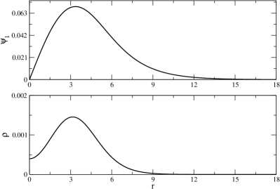
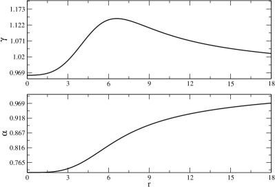
Figure 2: Self-gravitating $\ell$-boson star corresponding to point B in Fig. 1. Left panel: wave-function $\psi_{1}(r)$, and energy density $\rho(r)=(2\ell+1)\rho^{(\ell)}(r)/(8\pi)$, as functions of the radial coordinate. Right panel: the metric coefficients $\gamma(r)$ and $\alpha(r)$, also as a function of the radial coordinate. Notice that even though the wave-function vanishes at the origin, the energy density takes a value different from zero at that point. This is a characteristic of the $\ell=1$ configurations. See Fig. 3 for energy density profiles in the cases of $\ell=0$, 1 and 2. The regularity of these objects at the origin in evident in the profiles for the metric coefficients.

Configuration	$M$	$\;R(99\%)\;$	$\omega$	$M/R(99\%)$
A ($\ell=0$)	$\;0.63\;$	$7.89$	$\;0.854\;$	$0.08$
B ($\ell=1$)	$1.18$	$12.75$	$0.836$	$0.09$
C ($\ell=2$)	$1.72$	$15.35$	$0.832$	$0.11$
D ($\ell=3$)	$2.25$	$17.22$	$0.820$	$0.13$
E ($\ell=4$)	$2.78$	$19.80$	$0.819$	$0.14$

Table 1: Main characteristics of some $\ell$-boson stars with different angular momentum number, reported in Planck units. The labels A, B, C, D and E make reference to those in Fig. 1. Notice that the objects with a non-trivial angular momentum number are more compact than standard boson stars with $\ell=0$.

\begin{overpic}[width=208.13574pt]{rho.eps} \put(92.7,62.2){\includegraphics[scale={0.008}]{ell.eps}} \put(92.7,39.8){\includegraphics[scale={0.008}]{ell.eps}} \put(92.7,17.5){\includegraphics[scale={0.008}]{ell.eps}} \end{overpic}

\begin{overpic}[width=208.13574pt]{r2density.eps} \put(92.3,62.2){\includegraphics[scale={0.008}]{ell.eps}} \put(92.3,58.5){\includegraphics[scale={0.008}]{ell.eps}} \put(92.3,54.9){\includegraphics[scale={0.008}]{ell.eps}} \end{overpic}

Figure 3: Left panel: Profile of the energy density $\rho(r)=(2\ell+1)\rho^{(\ell)}(r)/(8\pi)$ for the configurations A, B, and C in Fig. 1, respectively. Notice that the vertical scale changes between the plots. It is interesting to emphasize that $\rho(0)\neq 0$ if $\ell=0$ or 1, but $\rho(0)=0$ if $\ell>1$. Only if $\ell=0$ the energy density takes its maximum value at the origin. Right panel: Same profiles as in left panel, but multiplied by the square of the areal radius. Even if the amplitude of the energy density decreases as the angular momentum number increases, the configurations become more extended, and then the combination $\rho r^{2}$ grows, leading to more massive objects; see Table 1 for details.

V Discussion and conclusions

We have introduced new solutions to the static EKG system of equations that describe regular self-gravitating objects of finite mass. These configurations incorporate some of the effects of angular momentum while keeping the spherical symmetry of the spacetime metric, generalizing standard non-rotating boson stars. The technique requires an arbitrary odd number $N$ of massive, complex, non-interacting scalar fields with an internal $U(N)$ symmetry, and are labeled by an angular momentum number, $\ell=(N-1)/2$, and the usual field amplitude and excitation number. This motivates the name $\ell$-boson star. In this paper we have restricted our attention to ground state configurations only, although this can be easily generalized to the case of excited states.

We have shown that these objects possess similar properties to those of standard $N=1$, $\ell=0$, boson stars. Specifically, for a given angular momentum number, the equilibrium configurations exhibit a maximum value of the mass, and this maximum grows as $\ell$ increases, leading to more compact objects. For the case of $\ell=0$, it is well known that the maximum mass configuration divides the stable and unstable branches. We have done some preliminary numerical evolutions for the case with $\ell=1$ and have found that the same appears to be true: for a given mass below the maximum, configurations with a large effective radius and higher frequencies (those to the right of the maximum in both panels of Fig. 1) remain stable when perturbed, while those with smaller effective radius and smaller frequencies (to the left of the maximum in Fig. 1) either collapse rapidly to a black hole, or oscillate with a very long period around a less compact state (depending on the precise way in which they are perturbed). We will report on the results of these simulations and those for $\ell>1$ elsewhere.

Even if in this paper we restricted our attention to the ground state $n=1$ and only one single value of $\ell$ at a time in the configurations, the system of Eqs. (7) can easily be generalized to the case when several different modes $(n,\ell)$ are present simultaneously. This can be achieved by summing over all the excited states in the right hand side of Eqs. (7a) and (7b), similarly to the multi-state configurations constructed in Bernal:2009zy ; UrenaLopez:2010ur for $\ell=m=0$. Under the classical approach that we assume in this paper, this requires the inclusion of more fields, making it possible to use not only odd, but also even values of $N$, and to obtain more general density profiles than those reported here. We leave a more detailed analysis for a companion paper.

The main implication of this work is that the solution space of spherically symmetric, static boson stars is much larger and has a much richer structure when a collection of scalar fields is considered instead of a single complex scalar field that necessarily requires of the harmonic $\ell=m=0$. An alternative interpretation for the collection of scalar fields considered here, and potential applications for dark matter observations, will be explored in another paper.

Appendix A Stress energy-momentum tensor for the collection of scalar fields given in Eq. (2)

The purpose of this appendix is to provide a proof for the statement regarding the fact that the stress energy-momentum tensor associated with a collection of scalar fields of the form in Eq. (2) is spherically symmetric. For an alternative proof based on methods from quantum mechanics, see the Appendix in Ref. Olabarrieta:2007di .

The proof here is based directly on the well-known identity

$$\sum\limits_{m=-\ell}^{\ell}|Y^{\ell m}(\vartheta,\varphi)|^{2}=\frac{2\ell+1}{4\pi},$$ (21)

which upon differentiation and taking into account that $(Y^{\ell m})^{*}=Y^{\ell-m}$, yields

$$\sum\limits_{m=-\ell}^{\ell}Y^{\ell m}(\vartheta,\varphi)^{*}\hat{\nabla}_{A}Y^{\ell m}(\vartheta,\varphi)=0.$$ (22)

Here and in the following, $\hat{\nabla}_{A}$ and $\hat{g}_{AB}$ refer to the covariant derivative and standard metric, respectively, on the unit two-sphere. Taking a further derivative gives

$$\sum\limits_{m=-\ell}^{\ell}(\hat{\nabla}_{A}Y^{\ell m})^{*}(\hat{\nabla}_{B}Y^{\ell m})=-\sum\limits_{m=-\ell}^{\ell}(Y^{\ell m})^{*}\hat{\nabla}_{A}\hat{\nabla}_{B}Y^{\ell m}.$$ (23)

Since $\hat{\nabla}^{A}\hat{\nabla}_{A}Y^{\ell m}=-\ell(\ell+1)Y^{\ell m}$, the trace of this equation together with Eq. (21) provide the following identity:

$$\sum\limits_{m=-\ell}^{\ell}(\hat{\nabla}^{A}Y^{\ell m})^{*}(\hat{\nabla}_{A}Y^{\ell m})=\frac{\ell(\ell+1)(2\ell+1)}{4\pi}.$$ (24)

On the other hand, taking the divergence on both sides of Eq. (23), and using Eq. (22), we obtain

$$\sum\limits_{m=-\ell}^{\ell}(\hat{\nabla}^{A}Y^{\ell m})^{*}\hat{\nabla}_{A}\hat{\nabla}_{B}Y^{\ell m}=0.$$ (25)

The previous formula implies that the symmetric trace-free tensor field on the two-sphere

$$\tau_{AB} := \sum\limits_{m=-\ell}^{\ell}\left[(\hat{\nabla}_{A}Y^{\ell m})^{*}(\hat{\nabla}_{B}Y^{\ell m})\right.$$ (26)

$$\left.\qquad-\frac{1}{2}\hat{g}_{AB}(\hat{\nabla}^{C}Y^{\ell m})^{*}(\hat{\nabla}_{C}Y^{\ell m})\right]$$

is divergence-free. However, all symmetric, trace- and divergence-free tensor fields on the two-sphere are trivial (see, for instance Lemma 1 in the Appendix of Ref. eCnOoS13 ), such that $\tau_{AB}=0$. This implies

$$\sum\limits_{m=-\ell}^{\ell}(\hat{\nabla}_{A}Y^{\ell m})^{*}(\hat{\nabla}_{B}Y^{\ell m})=\frac{\ell(\ell+1)(2\ell+1)}{8\pi}\hat{g}_{AB}.$$ (27)

Based on the identities (21–27), one easily finds the following expressions for the components of the stress energy-momentum tensor given in Eq. (II):

$$T_{ab} = \frac{2\ell+1}{4\pi}\left[(\partial_{a}\phi_{\ell})^{*}(\partial_{b}\phi_{\ell})-\frac{1}{2}\tilde{g}_{ab}\left(\tilde{g}^{cd}(\partial_{c}\phi_{\ell})^{*}(\partial_{d}\phi_{\ell})\right.\right.$$

$$\qquad\qquad\left.\left.+\frac{\ell(\ell+1)}{r^{2}}|\phi_{\ell}|^{2}+\mu^{2}|\phi_{\ell}|^{2}\right)\right],$$

$$T_{aB} = 0,$$ (28)

$$T_{AB} = -\frac{2\ell+1}{8\pi}r^{2}\left[\tilde{g}^{cd}(\partial_{c}\phi_{\ell})^{*}(\partial_{d}\phi_{\ell})+\mu^{2}|\phi_{\ell}|^{2}\right]\hat{g}_{AB},$$

where here $a,b=t,r$, $A,B=\vartheta,\varphi$ and $\tilde{g}_{ab}$ refers to the components of the time–radial part $-\alpha^{2}dt^{2}+\gamma^{2}dr^{2}$ of the metric.

References

- (1) D.J. Kaup, “Klein-Gordon geon,” Phys. Rev. 172, 1331 (1968)
- (2) R. Ruffini and S. Bonazzola, “Systems of selfgravitating particles in general relativity and the concept of an equation of state,” Phys. Rev. 187, 1767-1783 (1969)
- (3) M. Colpi, S.L. Shapiro and I. Wasserman, “Boson stars: Gravitational equilibria of selfinteracting scalar fields,” Phys. Rev. Lett. 57, 2485-2488 (1986)
- (4) R. Friedberg, T.D. Lee and Y. Pang, “Mini-soliton stars,” Phys. Rev. D 35, 3640-3657 (1987)
- (5) M. Gleiser, “Stability of boson stars,” Phys. Rev. D 38, 2376 (1988)
- (6) T.D. Lee and Y. Pang, “Stability of mini-boson stars,” Nucl. Phys. B 315, 477 (1989)
- (7) E. Seidel and W-M. Suen, ”Dynamical evolution of boson stars: Perturbing the ground state,” Phys. Rev. D 42, 384 (1990)
- (8) F.S. Guzman and L.A. Urena-Lopez, “Evolution of the Schrodinger-Newton system for a selfgravitating scalar field,” Phys. Rev. D 69, 124033 (2004) [arXiv:0404014 [gr-qc]]
- (9) P. Jetzer, “Boson stars,” Phys. Rept. 220, 163-227 (1992)
- (10) T.D. Lee and Y. Pang, “Nontopological solitons,” Phys. Rept. 221, 251-350 (1992)
- (11) F.E. Schunck and E.W. Mielke, “General relativistic boson stars,” Class. Quant. Grav. 20, R301-R356 (2003) [arXiv:0801.0307 [astro-ph]]
- (12) S.L. Liebling and C. Palenzuela, “Dynamical boson stars,” Living Rev. Rel. 15, 6 (2012) [arXiv:1202.5809 [gr-qc]]
- (13) D.F. Torres, S. Capozziello and G. Lambiase, “A Supermassive scalar star at the galactic center?,” Phys. Rev. D 62, 104012 (2000) [arXiv:104012 [astro-ph]]
- (14) F.G. Guzman, “Accretion disc onto boson stars: A Way to supplant black holes candidates,” Phys. Rev. D 73, 021501(R) (2006) [arXiv:0512081 [gr-qc]]
- (15) P. Amaro-Seoane, J. Barranco, A. Bernal, and L. Rezzolla, “Constraining scalar fields with stellar kinematics and collisional dark matter,” JCAP 1011, 002 (2010) [arXiv:1009.0019 [astro-ph.CO]]
- (16) C.J. Hogan and M.J. Rees, “Axion miniclusters,” Phys. Lett. B 205, 228-230 (1988)
- (17) E.W. Kolb and I.I. Tkachev, “Axion miniclusters and Bose stars,” Phys. Rev. Lett. 71 3051-3054 (1993) [arXiv:9303313 [hep-ph]]
- (18) J. Barranco and A. Bernal, “Self-gravitating system made of axions,” Phys. Rev. D 83, 043525 (2011) [arXiv:1001.1769 [astro-ph.CO]]
- (19) S-J. Sin, “Late time cosmological phase transition and galactic halo as Bose liquid,” Phys. Rev. D 50, 3650-3654 (1994) [arXiv:9205208 [hep-ph]]
- (20) H-Y. Schive, T. Chiueh and T. Broadhurst, “Cosmic structure as the quantum interference of a coherent dark wave,” Nature Phys. 10, 496-499 (2014) [arXiv:1406.6586 [astro-ph.GA]]
- (21) D.J.E. Marsh, “Axion cosmology,” Phys. Rept. 643, 1-79 (2016) [arXiv:1510.07633 [astro-ph.CO]]
- (22) L. Hui, J.P. Ostriker, S. Tremaine, E. Witten, “Ultralight scalars as cosmological dark matter,” Phys. Rev. D 95, 043541 (2017) [arXiv:1610.08297 [astro-ph.CO]]
- (23) I. Olabarrieta, J.F. Ventrella, M.W. Choptuik and W.G. Unruh, “Critical behavior in the gravitational collapse of a scalar field with angular momentum in spherical symmetry,” Phys. Rev. D 76, 124014 (2007) [arXiv:0708.0513 [gr-qc]]
- (24) G.H. Derrick, “Comments on nonlinear wave equations as models for elementary particles,” J. Math. Phys. 5 1252-1254 (1964)
- (25) A. Diez-Tejedor and A. Gonzalez-Morales, “No-go theorem for static scalar field dark matter halos with no Noether charges,” Phys. Rev. D 88, 067302 (2013) [arXiv:1306.4400 [gr-qc]]
- (26) P. Bizoń and A. Wasserman, “On existence of mini-boson stars,” Commun. Math. Phys. 215, 357-373 (2000) [arXiv:0002034 [gr-qc]]
- (27) A. Bernal, J. Barranco, D. Alic and C. Palenzuela, “Multi-state boson stars,” Phys. Rev. D 81 044031 (2010) [arXiv:0908.2435 [gr-qc]]
- (28) L.A. Urena-Lopez and A. Bernal, “Bosonic gas as a galactic dark matter halo,” Phys. Rev. D 82 123535 (2010) [arXiv:1008.1231 [gr-qc]]
- (29) E. Chaverra, N. Ortiz and O. Sarbach, “Linear perturbations of self-gravitating spherically symmetric configurations”, Phys. Rev. D 87, 0440154 (2013) [arXiv:1209.3731 [gr-qc]]