X-ray ionization of the intergalactic medium by quasars

Abstract

We investigate the impact of quasars on the ionization of the surrounding intergalactic medium (IGM) with the radiative transfer code CRASH4, now accounting for X-rays and secondary electrons. After comparing with analytic solutions, we post-process a cosmic volume ($\approx 1.5\times 10^{4}$ Mpc${}^{3}h^{-3}$) containing a ULAS J1120+0641-like quasar (QSO) hosted by a $5\times 10^{11}{\rm M}_{\odot}h^{-1}$ dark matter (DM) halo. We find that: (i) the average HII region ($R\sim 3.2$ pMpc in a lifetime $t_{f}=10^{7}$ yrs) is mainly set by UV flux, in agreement with semi-analytic scaling relations; (ii) a largely neutral ($x_{\textrm{HII}}<0.001$), warm ($T\sim 10^{3}$ K) tail extends up to few Mpc beyond the ionization front, as a result of the X-ray flux; (iii) LyC-opaque inhomogeneities induce a line of sight (LOS) scatter in $R$ as high as few physical Mpc, consistent with the DLA scenario proposed to explain the anomalous size of the ULAS J1120+0641 ionized region. On the other hand, with an ionization rate $\dot{N}_{\gamma,0}\sim 10^{57}$ s^-1, the assumed DLA clustering and gas opacity, only one LOS shows an HII region compatible with the observed one. We deduce that either the ionization rate of the QSO is at least one order of magnitude lower or the ULAS J1120+0641 bright phase is shorter than $10^{7}$ yrs.

1 INTRODUCTION

X-rays play a central role in astrophysics because they can penetrate the deepest layers of dense gaseous regions, inducing photo-chemistry and a complex chain of collisional ionizing processes (secondary ionization). Even in environments with a high column density of neutral hydrogen ($N_{\texttt{HI}}>10^{20}\textrm{cm}^{-2}$), X-rays can create extended and partially ionized regions where a substantial fraction of the primary ionizing energy is converted into secondary, high velocity photo-electrons. These fast, charged particles are then able to collisionally ionize or excite both the H and He components of the gas. Since the first studies of Dalgarno and collaborators (Dalgarno et al., 1963), X-rays have been recognized as a central agent regulating the gas chemistry in planetary atmospheres, supernova ejecta, and the interstellar medium.

Quasi-stellar object spectra, for example, show emission lines induced by X-rays entering the surrounding clouds of the host galaxy (Kallman, 1984, 2010) and easily escaping it into the IGM. These lines are an exceptional diagnostic tool of the physical state of the host galaxy ISM because they are very sensitive to temperature and gas electron density, and therefore they are impacted by secondary ionization.

Because of their large mean free path, X-rays can also leave a peculiar signature on the large scale of the intergalactic medium (IGM) by determining its temperature and ionization state (Venkatesan et al., 2001; Zaroubi et al., 2007; Ripamonti et al., 2008; Fialkov et al., 2014; Xu et al., 2014). At high redshift even a small contribution by X-rays sources could produce an initial ionization of the IGM and increase its temperature (Baek et al., 2010; Mesinger et al., 2013; Kakiichi et al., 2017; Meiksin et al., 2017; Ross et al., 2017; Madau & Fragos, 2017; Eide et al., 2018) above the value of the Cosmic Microwave Background, affecting the detectability of the 21-cm signal from neutral hydrogen in these remote epochs (Madau et al., 1997; Ciardi & Madau, 2003; Pritchard & Furlanetto, 2007; Pacucci et al., 2014; Ewall-Wice et al., 2016; Kern et al., 2017; Das et al., 2017; Semelin et al., 2017).

The present generation of radio-array facilities such as the LOw Frequency ARray (LOFAR), or the Mileura Wide-field Array (MWA), as well as the future Square Kilometre Array (SKA), are expected to have the sensitivity required to detect the signal (e.g. Pritchard & Furlanetto 2007) before the epoch of hydrogen reionization. The interpretation of these observations will require a precise theoretical modeling of the ionization and heating processes.

Secondary ionization is important also in more exotic processes, as the decay or annihilation of Warm and Cold Dark Matter occurring during the Dark Ages. Such processes have been proposed in recent years as an additional source of IGM pre-heating (e.g. see Valdés & Ferrara 2008; Valdés et al. 2010; Evoli et al. 2012 and references therein).

Theoretical models of radiative transfer (RT) require an accurate implementation of both photo-ionization and secondary ionization to correctly interpret the data provided by these new facilities, to increase the realism of both hydrogen and helium reionization simulations, and to make predictions of the temperature evolution of the intergalactic gas (e.g. Oh 2001; Venkatesan et al. 2001; Glover & Brand 2003; Baek et al. 2010; Venkatesan & Benson 2011; Ross et al. 2017).

Most of the photo-ionization codes in current active development (Ferland et al., 1998; Ercolano et al., 2008; Allen et al., 2008) already account for the soft X-ray contribution and include the effects of the secondaries by implementing different models of energy release by cascade of charged particles. Fitting functions valid for H and He cosmological mixtures not polluted by metals have been provided by Shull and Van Steenberg (Shull, 1979; Shull & van Steenberg, 1985) and are currently implemented, among others, in MAPPINGS III, CLOUDY (Ferland et al., 2013), MOCASSIN and the semi-numerical 21CMFAST code (Mesinger et al., 2011). Cosmological radiative transfer codes, accounting for time evolution as well (Ricotti et al., 2002; Baek et al., 2010; Wise & Abel, 2011; Friedrich et al., 2012; Jeon et al., 2014; Bryan et al., 2014; Lee et al., 2016) have also included the effects of secondaries, mainly preferring the Shull and Van Steenberg model with the prescriptions suggested by Ricotti et al. (2002), but did not explore the dependence of their results on alternative or more updated models of secondaries (see Appendices A and B of the present work.).

In this work we first introduce a novel implementation of the cosmological radiative transfer code CRASH (hereafter CRASH4) which self-consistently treats UV and X-ray photons by accounting for the physics of secondary ionization. As various models of this process available in the literature treat the physical problem with different approximations (see Appendix A), CRASH4 has been designed to embed any of them in a modular way, so that their impact on the code predictions can be easily assessed. Second, we benchmark the code predictions with a series of ideal tests investigating the impact of a bright quasar-like source on a surrounding homogeneous IGM; these test cases are essential to establish the average properties of both hydrogen and helium ionized regions.

Recent observations of the highest redshift quasars at $z\sim 7.5$ (Bañados et al., 2018) and $z\sim 7.1$ (Mortlock et al., 2011; Bolton et al., 2011) suggest that their surrounding IGM could be substantially neutral; the correct interpretation of their spectra requires a deep understanding of the structure and properties of their H$\,{\rm{\scriptstyle II}}$ regions and how they expand against collapsed structures present in the surrounding cosmic web. To this aim, we apply our code to a realistic case of a high redshift QSO surrounded by a neutral, well resolved IGM and we explore the evolution of the resulting ionized fronts as function of the source lifetime. The effects of both UV and X-rays photons on the IGM are then statistically analyzed by sampling the ionized volume with a large number of line-of-sights. Note that the results of the present work complement the findings of a companion paper (Kakiichi et al. 2017, KK17), based on the same CRASH4 code, but investigating the case of a higher redshift quasar surrounded by star forming galaxies. KK17 suggests that galaxy surveys, performed on a region of sky imaged by 21 cm tomography, could help disentangling the relative role of QSOs and galaxies in driving cosmic reionization. This last problem is also addressed with CRASH4 by performing large scale reionization simulations (see Eide et al. 2018).

The present work is organized as follows. A general overview of CRASH4 is provided in Section 2, where we also briefly introduce the soft X-ray band and the secondary ionization process. In Section 3, we provide an extensive series of tests to show the code reliability and flexibility in simulating different physical environments. A first application to a QSO environment is shown in Section 4 and the dependence of the results on the adopted model of secondaries is fully discussed in the related appendices. The paper conclusions are summarized in Section 5.

2 CRASH4 overview

The aim of the new release of the radiative transfer code CRASH (Ciardi et al., 2001; Maselli et al., 2003, 2009a; Graziani et al., 2013; Hariharan et al., 2017), is the implementation of a new RT scheme capable to simulate simultaneously the radiative transfer in many spectral bands: the Ly$\alpha$ spectral line, the Lyman-Werner band, the UV and soft X bands, and finally the energies up to the non-relativistic gamma rays limit. In the present work we focus on the implementation of the soft X-ray band ($E_{\gamma}\sim 200$ eV - 3 keV) and on the description of the secondary ionization models necessary to compute the gas ionization and temperature.

Since its first release, CRASH is able to simulate the hydrogen and helium photo-ionization induced by UV radiation ($E_{\gamma}\in[13.6-200]$ eV) emitted from point sources and/or a background. The emission scheme of the code has been progressively enhanced by introducing a better sampling of the spectral distribution, an accurate treatment of the gas temperature (see Maselli et al. 2009a) and, finally, by treating the resonant propagation of $\textrm{Ly}\alpha$ photons self-consistently with the ionizing continuum (Pierleoni et al., 2009). The last global release of CRASH focused instead on implementing ionization of atomic metals self-consistently with the RT scheme (Graziani et al., 2013) and the optional integration in galaxy formation hybrid pipelines (Graziani et al., 2015; Graziani et al., 2017). The introduction of metals, which are ionized both at energies below the H$\,{\rm{\scriptstyle I}}$ ionization potential (e.g. Si$\,{\rm{\scriptstyle I}}$) and at X-rays energies (e.g. O$\,{\rm{\scriptstyle VII}}$), has highlighted the need for extending the RT to a wider spectral range.

As several separate implementations of CRASH already solve the RT in different energy bands (e.g. Pierleoni et al. 2009), CRASH4 should be considered as the convergent release of the many code streams and has already allowed the extension of the RT scheme through dust polluted regions (Glatzle et al., submitted). The large set of new physical effects introduced by CRASH4, combined with a consistent and unified development of all its modules, provides more realism to reionization simulations accounting for different source types (KK17, Eide et al. 2018) and it is crucial to advance previous models of QSO regions (Maselli et al. 2004, Maselli et al. 2007 (hereafter AM07), Maselli et al. 2009b), often limited to the investigation of hydrogen only I-fronts created by a UV flux.

The new multi-spectral-band RT scheme required a novel strategy capable of increasing the computational complexity while maintaining the flexibility of the algorithm. By increasing the code modularization and introducing many layers of parallelism, we implemented each spectral band in a separate threaded module. The ensemble of these new cooperative modules is organized into a new code library (Radiative Transfer Library for Cosmology, hereafter RT4C). Each RT4C module also handles the new physics induced in the gas by photo-ionization in a specific spectral band (e.g. secondary ionization induced by X-rays) and provides the necessary extensions to the equations of ionization and thermal evolution.

As more details on the algorithm can be found in previous CRASH papers, here we just provide the basic information necessary to understand the details of the new implementation.

A CRASH4 run consists of emitting photon packets from ionizing sources present in the computational domain and following their propagation through a Cartesian grid of $N^{3}_{c}$ cells. At each cell crossing, CRASH evaluates the absorption probability for a single photon packet as $(1-e^{-\tau})$ and derives the corresponding number of photons absorbed in the cell as:

$$N_{abs}=N_{\gamma}(1-e^{-\tau}),$$ (1)

where $N_{\gamma}$ is the photon content of the packet entering the cell and

$$\tau=\sum_{i}n_{i}\sigma_{i}l,$$ (2)

is the gas optical depth in the cell due to the contribution of all chemical species $i$. $n_{i}$ is then the number density of species $i$, $\sigma_{i}$ is its photo-ionization cross section (PCS), and $l$ is the path casted in the cell by the crossing ray. For an easier reading, we have omitted the frequency dependency of $\sigma_{i}$, $\tau$ and $N_{abs}$ but it is important to note that the algorithm propagates photon packets (i.e. collection of photons ad different frequencies distributed according to the intrinsic source spectral shapes of the sources (Maselli et al., 2009a)). For this reason the method is intrinsically multi-frequency in each considered spectral band and all the above quantities have an explicit dependence on photon energies. $N_{abs}$ is used to compute the contribution of photo-ionization and photo-heating to the evolution of the various species and the gas temperature $T$. We remind here that the current ray tracing scheme relies on the infinite speed of light approximation (see Appendix D).

To properly extend the above scheme to the soft X-ray band, it is necessary to ensure that the PCS adopted for each ionized species (e.g. H, He and metals ions) are coherently computed as function of the photon energies and maintain the required precision in all the spectral bands accounted for. Note that this fundamental atomic data is generally provided as fitting functions combining predictions of complementary theoretical methods constrained on experimental data. For example, Verner et al. (1993); Verner & Yakovlev (1995) showed that their Hartree-Dirac-Slater calculations are very reliable for inner atomic shells while result less accurate at lower energies, especially for low ionized or neutral species. Calculations based on the higher level R-Matrix method (Berrington et al., 1974; Berrington et al., 1987; Burke et al., 2006) are available in the Opacity and IRON projects (Seaton et al., 1992; Badnell et al., 2005; Seaton, 2005)) and provide more accurate predictions in the low energy regime, i.e. near the thresholds of atomic outer shells.

It is then important for multi-frequency RT codes computing the ionization of astrophysical plasma, to rely on a coherent set of atomic PCS. CRASH4 adopts PCS for hydrogen and helium provided in Verner et al. (1996) .

The inclusion of secondary ionization effects and heating by secondary electrons is described below and in Appendix A and B. The electron released by a photo-ionization event at frequency $\nu$ and requiring a potential $E_{\textrm{th}}$, carries a kinetic energy $E_{k}=(h\nu-E_{\textrm{th}})$, which could be enough to induce ionization by collisions in the surrounding gas, as well as to excite and heat it. The efficiency of this process is generally modeled as a function of $E_{k}$ and of the pre-existing ionization state of the gas $x_{e}\equiv n_{\textrm{e}}/n_{\textrm{gas}}$, where $n_{\rm e}$ and $n_{\textrm{gas}}$ are the electron and gas number density, respectively. Recent numerical calculations provide tabulated values of the number of secondary ionizations per species $i$, $N_{s,i}(E_{k},x_{e})$, and of the fraction $f_{Q}(E_{k},x_{e})$ of the photo-electron energy $E_{k}$ contributing to the gas heating.

For each species $i$, the ionization contribution from secondary electrons ($\delta x_{i}$) can be evaluated as $\delta x_{i}\propto N_{abs}N_{s,i}(E_{k},x_{e})$, where $N_{abs}$ is defined in Eq. 1. Similarly, the contribution to the photo-heating of a cell can be evaluated as $\delta T=E_{k}f_{Q}(E_{k},x_{e})$.

In CRASH4 we implement tables provided by three recent models of secondary ionization: Shull & van Steenberg (1985, hereafter SVS85), Dalgarno et al. (1999, hereafter DG99) and Valdés & Ferrara (2008, hereafter VF08). While SVS85 is the most widely used in the literature, DG99 has a more accurate treatment of some micro-physical processes and allows a future integration of the H2 component in the gas mixture. Finally, VF08 provides an updated implementations of atomic data present in the literature, and fitting formulas valid also in the hard X and gamma spectral bands (Valdés et al., 2010). While all the above models are in global agreement for photon energies above 100 eV (see Appendix A), their different implementation makes them complementary. DG99, for example, explicitly treats the H2 component and photons with energies below 100 eV, and it is the ideal choice when the impact of both Lyman-Werner and ionizing bands is accounted for. VF08 provides instead an estimate of the Ly$\alpha$ re-emission triggered by high energy photons and should be selected when Ly$\alpha$ flux becomes a crucial aspect of the investigation.

Before moving to a description of the results of this implementation, here we highlight that the conversion of the energy of secondary electrons into ionization is more efficient in a neutral or very poorly ionized gas, while as $x_{e}$ increases, an increasingly larger fraction of the initial electron energy is converted into heating or excitation. We refer the reader to Appendix A for more details on the effects of secondary electrons, on the model-dependent function $N_{s,i}(E_{k},x_{e})$, and on assumptions of the different models implemented in CRASH4.

Finally, we note that, although the code allows for it, the radiation emitted from recombining gas has not been explicitly followed in these tests; then the effect of the soft X-ray component should be considered as a lower limit.

3 Ideal ionized regions

Here we present a series of tests designed to verify the correct implementation of the X-ray physics in CRASH4, and the resulting implications. Appendices A, B and C provide analogous tests performed with different ionization models and in different pre-ionization configurations. Finally, the time evolution of these regions and the implications of adopting the infinite speed of light approximation are discussed in Appendix D.

We compute the properties of the ionized sphere created by a QSO-type, isotropic, point source embedded in a box of $110h^{-1}$ Mpc comoving (cMpc) at redshift $z=7.08$ (i.e. $\sim 19.0$ physical Mpc (pMpc or simply Mpc) by assuming $h=0.72$). The domain is mapped on a Cartesian grid of $N_{c}^{3}=512^{3}$ cells and the source is placed at the box corner (1,1,1). As basic set-up we consider a source with ionization rate $\dot{N}_{\gamma,0}=1.36\times 10^{56}$ photons s^-1 and a power-law spectral shape $S(\nu)\propto\nu^{-1.5}$ . The source spectrum extends up to $E_{\textrm{max}}=3$ keV and it is sampled by $N_{f}=41$ frequency bins, which are reduced if a cut to lower energies is applied (see next section for more details). The source emission is sampled by $N_{p}=2\times 10^{8}$ photon packets throughout the duration of the simulation, $t_{f}=10^{8}$ yrs. This choice ensures a Monte Carlo convergent solution as verified by repeating the run with a number of packets increased by one order of magnitude. The gas is assumed to be homogeneous (with a number density $n_{\textrm{gas}}=9.59\times 10^{-5}$ cm^-3), neutral, and at an initial temperature $T_{0}=100$ K. All the values indicated above have been selected in light of a direct comparison with the realistic case investigated in Section 4 and consistent with parameters adopted in AM07 and Bolton et al. 2011.

3.1 Hydrogen only

In this section we describe the H$\,{\rm{\scriptstyle II}}$ region created in a gas composed by atomic hydrogen only. For this set-up we choose DG99 because it is the only model describing a configuration with pure H, while SVS85 and VF08 are designed to account for a cosmological gas mixture of H and He.

The spherically averaged profile of $x_{\textrm{HII}}$ at the intermediate time $t_{i}=6\times 10^{7}$ yrs is shown in the top panel of Figure 1, as obtained by cutting the assigned spectral shape up to different values of $E_{\gamma}$: $0.1$ keV (i.e. $E_{\gamma}\in[13.6-100]$ eV, dashed-double-dotted red line), 0.2 keV (dashed-dotted red line), $E_{\gamma}=0.5$ keV (triple-dotted red line) and finally a full case including photons with energies up to 3 keV (solid blue line). All the profiles account for the contribution of direct photo-ionization and secondary processes. Finally a case with maximum energy $E_{\gamma}=3.0$ keV but excluding the contribution of secondary ionization is shown as dashed black line. In each case the location of the I-front remains the same and corresponds to $d\sim 2.0$ physical Mpc, indicating that the UV radiation below $E_{\gamma}=0.1$ keV plays the most important role in establishing the gas full ionization.

Photons with $0.1$ keV $<E_{\gamma}<0.2$ keV induce instead a substantial difference in the external part of the H$\,{\rm{\scriptstyle II}}$ region (2.0 Mpc $<d<4.0$ Mpc), while the soft X-ray component is mainly supporting the tail at distances $d>4.0$ Mpc. Their highly penetrating flux creates then a large and diffuse low-ionization shell with $0.0001<x_{\textrm{HII}}<0.003$. As a reference, the comoving mean free path $\lambda_{X}$ of an X-ray photon with $E_{\gamma}=1$ keV in a H-only neutral IGM ($\bar{x}_{\textrm{HI}}\sim 1$) at $z=7.08$, is $\lambda_{X}=4.9\times\bar{x}_{\textrm{HI}}^{-1/3}((1+z)/15)^{-2}(E_{\gamma}/300\leavevmode\nobreak\ {\rm eV})^{3}=625$  cMpc, i.e. 77 pMpc (see Furlanetto et al. 2006; Pritchard & Loeb 2012). At $d>2.0$ Mpc, the efficiency of secondary electrons in ionizing the gas is also evident, increasing the ionization fractions of about one order of magnitude compared to a case without secondaries and maintaining the extreme tail of the profile up to $d\sim 8$ Mpc. It is important to note here that by disabling secondary ionization the code removes this effect at all photon energies, as imposed by the model in DG99. This is the reason why the dashed black line (i.e. without secondaries) corresponds to values lower than the dashed-dotted red line. It is also evident, by comparing the 0.2 keV and 0.1 keV cases, that part of the photons with $E_{\gamma}>0.1$ keV contributes in creating the external tail discussed above, as the efficiency of the secondary ionization process has no activation thresholds but increases with the photon energy (see Appendix A for more details).

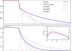
Figure 1: Radial profiles of $x_{\textrm{HII}}$ (top panel) and log$(T)$ (bottom) of the Strömgren sphere created in a gas made of neutral atomic hydrogen at the simulation time $t_{i}=6\times 10^{7}$ yrs, and adopting the DG99 model. The distance $d$ from the source is shown in physical Mpc. In all the panels the profiles are created by a spectrum extending up to: $E_{\textrm{max}}=3$ keV, with/without the effect of the secondary electrons (blue solid/black dashed line). The dashed-double-dotted red line indicates the profile created by cutting the energy at $E_{\textrm{max}}=0.1$ keV, the dashed-dotted red at $E_{\textrm{max}}=0.2$ keV, while the triple-dotted red line refers to a cut at $E_{\textrm{max}}=0.5$ keV. The small box in the bottom panel shows a zoom of the gas temperature (in linear scale of $10^{4}$ K) in the fully ionized region 0.1 Mpc $<d<1.9$ Mpc.

The bottom panel of Figure 1 shows the corresponding temperature profiles. Similarly to $x_{\rm HII}$, also the temperature inside the I-front ($T\sim 4.0\times 10^{4}$ K) is mainly determined by the effect of photons with $E_{\gamma}<0.1$ keV, while higher energy photons in the spectrum induce a remarkable gas heating in the external shell ($2.0$ Mpc$<d<2.9$ Mpc), where $T\geq 10^{3}$K. A zoom-in view of the radial distribution of $T$ in $0.1$ Mpc $<d<1.9$ Mpc is given in the panel inset, where we show the temperature values in linear scale to better understand the contribution of secondaries in subtracting energy to the gas photo-heating. Also note that even at larger distance (corresponding to $d>3.5$ Mpc) the temperature is maintained at values above $T_{0}=100$ K.

When secondary ionization is switched off, all the kinetic energy of the fast electrons goes into gas heating rather than being distributed between heating and ionization; the resulting gas temperature is then higher than in the case with secondaries. By comparing the red lines, the contribution to the gas heating by photons with $E_{\gamma}<0.2$ keV becomes evident (also see panel inset).

3.2 Hydrogen and helium

We now discuss the ionized spheres obtained in a gas composed by hydrogen (number fraction 0.92) and helium (number fraction 0.08). We adopted the DG99 model because it is the only one explicitly accounting for the effects of secondary ionization on $x_{\rm HeIII}$. A discussion of the differences induced by using the other models (SVS85 and VF08) can be found in Appendix B.

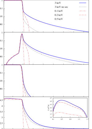
Figure 2: Radial profiles of the Strömgren sphere created in a cosmological mixture of H and He at the simulation time $t_{i}=6\times 10^{7}$ yrs, and adopting the DG99 model. The distance $d$ from the source is shown in physical Mpc. In all the panels the profiles are created by a spectrum extending up to: $E_{\textrm{max}}=3$ keV, with/without the effect of the secondary electrons (blue solid/black dashed line). The dashed-double-dotted red line indicates the profile created by cutting the energy at $E_{\textrm{max}}=0.1$ keV, the dashed-dotted red at $E_{\textrm{max}}=0.2$ keV, while the triple-dotted red line refers to a cut at $E_{\textrm{max}}=0.5$ keV. From the top to the bottom the panels refer to the profiles of $x_{\textrm{HII}}$, $x_{\textrm{HeII}}$, $x_{\textrm{HeIII}}$ and log$(T)$. The small box in the bottom panel shows a zoom of the gas temperature (in linear scale of $10^{4}$ K) in the fully ionized region $0.1<d<1.7$ Mpc. See text for more details.

In Figure 2 we show the results of this test. The location of the I-front of $x_{\textrm{HII}}$ is similar to the pure H case, indicating that helium does not substantially alter the ionization of the inner region. On the other hand, the partially ionized shell at $d>2.0$ Mpc created by photons with energy $E_{\gamma}\in[0.1-0.2]$ keV is reduced in size because He$\,{\rm{\scriptstyle I}}$ and He$\,{\rm{\scriptstyle II}}$ provide an important contribution to the optical depth even at the lowest energy cuts.

The qualitative agreement found with Figure 1 indicates that the presence of secondary electrons primarily affects the hydrogen component, which is more abundant and can easily support low hydrogen ionization $x_{\textrm{HII}}<0.001$ up to 8 Mpc.

The second and third panels from the top show the profiles of $x_{\textrm{HeII}}$ and $x_{\textrm{HeIII}}$, respectively. The location of the I-fronts of $x_{\textrm{HeII}}$ and the size of the partially ionized shells are similar to those of $x_{\rm HII}$. This result depends on the spectral shape index chosen for this test. By comparing the solid and dashed lines in the first three panels, we can confirm the dominant role of the secondaries in maintaining the external shell at low ionization, although their effect is less significant than for hydrogen. Neutral He is then more sensitive to direct photo-ionization by X-rays photons than to secondary ionization. The X-ray component has an impact also on the $x_{\textrm{HeIII}}$, although smaller than on the other profiles. A little role (similar to what is found for $x_{\rm HeII}$) is also played by the secondaries in maintaining the partial ionization level of the outer region (compare dashed and solid lines).

The bottom panel finally shows the temperature profiles. Here again, the major differences induced by the presence of X-rays are found in the shell outside the I-front: while the inner region is maintained at a temperature $T\sim 4.2\times 10^{4}$ K , the outer shell has temperatures in the range $10^{3}$ K$<T<10^{4}$ K up to a distance of $d\sim 2.5$ Mpc, i.e. the end of the $x_{\textrm{HeIII}}$ profile. The initial temperature $T_{0}=100$ K is finally restored after a long and smoothly decreasing tail corresponding to the decrease of the $x_{\textrm{HII}}$ ionization profile. A zoom of the temperature behavior in the fully ionized region is provided also for this configuration. Here the contribution of photons with $0.1$ keV $<E_{\gamma}<0.5$ keV is more evident as they mainly interact with the helium component (compare solid and dashed-dotted/dashed-double-dotted lines). Photons with energies $E_{\gamma}>0.5$ keV do not affect the heating of the inner region as their profile overlaps with the solid blue line. Finally, note that when helium is included the energy is distributed in a more complex way across the three ions. For example, we note that the temperature of the low ionization tail obtained by disabling the secondary ionization (black dashed line) is lower than in the case with X-rays (solid blue) and does not have a straightforward interpretation. Here two effects combine: (i) the He column density is lower than the H one, and thus the collisional ionization probability on atoms of helium results one order of magnitude lower (see blue lines in Figures A1, A2, Appendix A), and (ii) at X-ray frequencies the photo-ionization cross section of neutral helium is about one order of magnitude higher than the one of hydrogen.

We have repeated the test presented above in a range of gas number density ($n_{gas}\in[10^{-2},10^{-5}]$ cm^-3), source ionization rates ($\dot{N}_{\gamma,0}\in[10^{54}-10^{57}]$  photons s^-1) and non neutral initial conditions $x_{0}$ ($x_{\textrm{0,HII}}=x_{\textrm{0,HeII}}=x_{0}\in[10^{-4}-2\times 10^{-1}]$ and $x_{\textrm{0,HeIII}}=0$) to verify that the qualitative results illustrated above are not numerical artifacts nor features restricted to a specific set-up. As expected, we found a similar behavior in all configurations. Quantitatively though, there are differences with e.g. the size of the partially ionized shell strongly depending on $x_{0}$ as detailed in Appendix C. On the other hand, the location of the I-front remains the same as long as $x_{0}<0.1$, while it progressively moves away from the source with increasing $x_{0}$. In realistic cases, involving many sources and an in-homogeneous gas distribution, the problem becomes strongly model-dependent.

To summarize the results of this section, the presence of X-rays creates an extended region at low ionization and temperatures up to $10^{3}$ K, which is not present at photon energies $E_{\gamma}<0.1$ keV. This feature is confirmed by all the models of secondary ionization (see Appendix B), even if the internal structure of the ionized shell can significantly change from one model to another.

4 IGM ionization by quasars

In this section we consider a QSO-like source at $z\sim 7.08$ embedded in a massive halo, in analogy with Bolton et al. (2011). The gas distribution is simulated using the code GADGET3 (Springel, 2005) in a box of comoving size 25 Mpc $h^{-1}$, chosen so that the most massive halo at $z\sim 7.08$ (with a total mass of $\sim 5\times 10^{11}$ M${}_{\odot}h^{-1}$, $R_{vir}\sim 292.2$ ckpc $\sim 36.2$ kpc physical) is located in a corner of the box. The simulation employs $2\times 512^{3}$ gas and dark matter particles, resulting in a particle mass resolution of $1.50\times 10^{6}{\rm M}_{\odot}h^{-1}$ and $6.91\times 10^{6}{\rm M}_{\odot}h^{-1}$, respectively, and a gravitational softening length of 1.628 kpc$\leavevmode\nobreak\ h^{-1}$. The outputs of this hydrodynamical simulation are mapped onto a grid of $N_{c}^{3}=512^{3}$ cells and post-processed with CRASH4. The resulting spatial resolution is $d\sim 48.8h^{-1}$ ckpc, i.e. $\sim 8.4$ physical kpc.

We place our source within the most massive halo located in the grid corner (1,1,1), and consider the emission in a quadrant angle. The gas mixture is composed by hydrogen and helium in cosmological fractions and we only consider the case of an initial neutral gas configuration; this set-up allows us to understand the contribution of the gas inhomogeneities in enhancing or suppressing the features found in the test cases. In the reference run the source emissivity is $\dot{N}_{\gamma,0}=1.36\times 10^{56}$ photons s^-1 as in the ideal tests to allow a direct comparison. In addition, we also investigate the implications of a higher value $\dot{N}_{\gamma,1}=1.36\times 10^{57}$ photons s^-1, consistent with the ionization rate estimated for the high redshift quasar ULAS J1120+0641 (Mortlock et al., 2011), while the other parameters are the same as in the previous section. The effects of the two ionization rates in a uniform medium are discussed in Appendix B (see also Keating et al. 2015).

For this study we adopt a full spectrum including X-rays with energies up 3 keV and the VF08 model of secondary ionization, providing the most updated treatment of the atomic coefficients and the most recent modeling of collisional processes induced by secondaries (see Appendix A and B for more information). The simulation starts assuming the gas as neutral and takes as initial temperature $\bar{T}_{0}$ the average value of $\sim 100$ K provided by the gas hydrodynamics. The simulation duration is set up to $t_{f}=10^{8}$ yrs, with results stored at intervals of $\Delta t=10^{7}$ yrs, consistent with an average quasar lifetime (see Khrykin et al. 2016 for a recent estimate at lower redshift). This set-up significantly improves a series of previous studies (e.g. AM07) both in the spatial resolution, in the accuracy of the RT physics and in the derived properties of the IGM (i.e. its ionization and temperature). It should be noted that old treatments of RT were computationally limited to a shorter UV range (AM07 uses $E_{\gamma}\in[13.6-42]$ eV) appropriate for computations with hydrogen only, while CRASH4 is designed to overcome these limitations and to provide a more realistic description of the multi-frequency RT through cosmic mixtures. As final remark we point out that this set-up does not consider any previous reionization history; we defer the discussion of this important point to the companion work KK17.

4.1 Average properties of the ionized region

To understand the impact of the quasar on the simulated volume, we first summarize the average properties of the HII region at an intermediate time $t_{i}=6\times 10^{7}$ yrs and at the end of the simulation $t_{f}=10^{8}$ yrs. The volume average hydrogen ionization fractions are $\bar{x}_{\textrm{HII}}\sim 0.162$ and $\bar{x}_{\textrm{HII}}\sim 0.274$, with a minimum value in the simulated volume of about $x_{\textrm{HII}}\sim 3\times 10^{-4}$ in both cases. These values clearly indicate that (i) the fully ionized region involves only $\sim 15$% (30 %) of the simulated volume and its impact on the ionization of the neutral IGM is limited in space, (ii) the X-ray flux pervades the entire cosmological box impacting gas far from the fully ionized fronts. Similar considerations can be applied to the helium component, which results fully ionized in 12 % (20 %) of the volume and is never completely neutral, clearly indicating the presence of high energy photons at the end of the simulated volume. Consistently with these findings, the volume-averaged gas temperature is almost in photo-ionization regime, $\bar{T}\sim 5.5\times 10^{3}$ $(\sim 8.5\times 10^{3})$ K, with a large spread from $T_{\textrm{max}}\sim 4.0\times 10^{4}$ $(\sim 8.4\times 10^{4})$ K down to $T_{\textrm{min}}\sim 115$ K (a negligible heating for the scope of the present work). The spherically-averaged profiles of the ionized region are similar to the profiles found in the previous section, predicting an I-front position around $d\sim 2.61$ $(\sim 3.2)$ physical Mpc, which is consistent with semi-analytic estimates of a sphere radius $R_{s}$ (derived by Cen & Haiman 2000; Madau & Rees 2000 and further discussed in White et al. 2003):

$$R_{s}=7.0\mathrm{\,pMpc}\left(\frac{\dot{N}_{\gamma,0}}{10^{58}\mathrm{s^{-1}}}\frac{t_{s}}{10^{7}\mathrm{yr}}\right)^{\nicefrac{{1}}{{3}}}\left(\frac{1+z}{7.37}\right)^{-1},$$ (3)

yielding $R_{s}=2.77$ $(3.3)$ physical Mpc, when computed for values appropriate to our simulation. These estimates, though, can not account for the effects of X-rays outside the I-front and can not describe the large oscillations revealed along different LOSs. These are discussed in the next section.

4.2 Direction-dependent ionized region size

To analyze the impact of the cosmic web on the structure of ionization fronts, we draw $10^{6}$ random LOS from the central source; we also checked that their casted path captures both the hydrogen and helium I-fronts and the long partially ionized tail. We start discussing the longest/shortest LOS (LOS A/LOS B) I-front found at the reference time $t_{i}=6\times 10^{7}$ yrs and at the end of the simulation, while the statistical properties of the sample are presented at the end of the section.

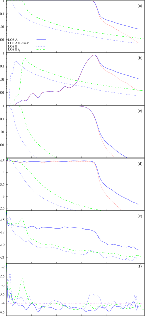
Figure 3: The most (LOS A, blue solid lines) and the least (LOS B, blue dashed lines) extended ionization profile in the realistic ionized region created around the QSO considered in Section 4. Red lines with same linestyle refer to the same LOS profiles derived from a simulation performed with a spectrum cut at 0.2 keV. The lines refer to the simulation time $t_{i}=6\times 10^{7}$ yrs and the distance $d$ from the source is shown in physical Mpc. The green dashed-dotted line refers instead to the LOS B (UV+X) found in the same simulation at the final time $t_{f}=10^{8}$ yrs. From the top to the bottom the panels refer to the profiles of $x_{\textrm{HII}}$, $x_{\textrm{HeII}}$, $x_{\textrm{HeIII}}$, log$(T)$, log$(\gamma)$ and log$(n_{gas})$. The horizontal line in the bottom panel indicates the volume average value of the gas number density in the adopted hydro-dynamical snapshot.

Figure 3 shows LOS A/LOS B in both $E_{\gamma}=3.0$ keV and $E_{\gamma}=0.2$ keV spectrum configurations, together with the corresponding profiles of temperature, gas recombination rate ($\gamma$) and number density. It is immediately evident that the position of the hydrogen I-fronts of the two LOSs differs by $-92$% and $+26$% from the semi-analytic estimate $R_{s}\sim 2.77$. These differences are mainly due to the high number density present in the inner region of the halo (corresponding to over-densities $\Delta=n_{\textrm{gas}}/\bar{n}_{\textrm{gas}}>100$) and the various gas structures found along each LOS, as seen in panel (f). Note that the global shape of the profiles is broadly similar to that of spherically averaged profiles (see Appendix B and compare with Figure B1), while significant spatial $x_{\textrm{HeII}}$ oscillations are induced by the underlying density distribution.

At $t=6\times 10^{7}$ yrs the I-front of LOS B is trapped within $d\sim 0.2$ Mpc, as photons with energies lower than 0.2 keV cannot escape the inner over-density (for this reason its line is not visible in the plot), while X-rays can travel up to end of the box and create a smoothly declining profile at low ionization ($0.0001<x_{\textrm{HII}}<0.01$), which extends up to $d\sim 5$ Mpc. A similar interpretation applies to LOS A, intercepting a smoother gas distribution (mostly under-dense) and consequently finding its I-front pushed away by $\sim 3.5$ physical Mpc.

These differences are mainly due to photons $E_{\gamma}<0.2$ keV (UV regime), while the X-rays photons create an extended layer of ionized hydrogen at $0.1<x_{\textrm{HII}}<0.001$ with extension $d\sim 4.5$ Mpc, physical. For both LOSs, the external region of the box is characterized by values $x_{\textrm{HII}}\leq 10^{-3}$. As in the ideal tests (refer for e.g. to Figure 2), low ionization is produced by secondary electrons, whose effects are modulated by variations of the recombination rate associated with gas density peaks (see panel (e)).

Similarly to hydrogen, the $x_{\textrm{HeII}}$ profiles become more extended due to X-rays, while the fully ionized helium is hardly affected, as it depends mainly on the UV flux.

The temperature profiles are shown in panel (d) of Figure 3. Note, for LOS A, the presence of a long tail at $T\sim 10^{3}$ K extending up to $d\sim 4.5$ Mpc, and temperatures as high as $T\sim 500$ K found up to distance $d\sim 6$ Mpc; beyond this distance the gas has not been reached by photons and its temperature is at $\bar{T}_{0}$. This is a clear indication that the X-ray heating in the region surrounding the QSO is not negligible. The gas temperature of LOS B follows the same trend and decreases below $T\sim 10^{4}$ K at $d>0.5$ Mpc. Note, on the other hand that it remains above $T=10^{3}$ K up to $d\sim 1.5$ Mpc indicating substantial heating by X-ray photons. The initial temperature is finally restored at distances $d>2.5$ Mpc.

We performed the previous analysis at the simulation end ($t_{f}=10^{8}$ yrs) to investigate the front displacement, finding a similar relative scatter ($\sim 4$ Mpc). LOS B at $t_{f}$ shows that UV photons are stopped by over-densities ($\Delta>30$) present within 1 Mpc (see Figure 3, dashed-dotted green line). Depending on the assumed QSO lifetime, systems clustering around the QSO can then significantly shape its I-front and change its impact on the surrounding IGM (see also KK17). More quantitatively, we find that 0.5 % of our I-fronts stop within 2 Mpc while only $\sim 9$ % within 3 Mpc. Despite their effectiveness in trapping the UV flux, the probability of observing a radius smaller than $R_{s}$ is then very low, at least within the adopted clustering.

For a better comparison with the case of ULAS J1120+0641, in the following we investigate how the least extended LOS changes by adopting $\dot{N}_{\gamma,1}=1.36\times 10^{57}$ s^-1 and a lifetime $t_{i}=10^{7}$ yrs. In this case LOS B shows an I-front at $d\sim 1.7$ Mpc and it is particularly remarkable as it is created by a sudden increase of $n_{\textrm{gas}}$ corresponding to a series of collapsed structures with gas over-density $\Delta>100$. In the left panel of Figure 4 we show the cosmic web in a slice cut intercepting this region (dashed white square). By visualizing the gas distribution we verified that there is an intricate structure in which many filaments cross. Many systems with column densities $19\leq\log(N_{\textrm{gas}}/{\rm cm}^{-2})<21$ are found in this region. The I-front of LOS B can be easily identified as the feature traced by the iso-contour lines of $x_{\textrm{HII}}$ in decreasing value, from red (0.99996) to blue (0.015). A zoomed-in view of the region of interest is given in the four panels on the right side of the same figure. Here the gas ionization profiles of both hydrogen and helium are shown, as well as the gas temperature. The simultaneous presence of DLA ($N_{\textrm{gas}}\sim 4\times 10^{20}$ cm^-2 as well as many Lyman limit systems (i.e. more than 35 systems with $19.9\leq\log(N_{\textrm{gas}}/{\rm cm}^{-2})\leq 20.3$ in the cubic region relative to the zoomed-view) causes the front to drop sharply both in $x_{\textrm{HII}}$ and $T$. Consistently, the fully ionized helium front is found at shorter distances, being more sensitive to the gas over-densities via recombinations. This picture is remarkably consistent with the QSO properties observed by Mortlock et al. (2011) and the DLA scenario proposed in Bolton et al. (2011) for the interpretation of the HII region size. The spectrum of ULAS J1120+0641, exhibits in fact a Ly$\alpha$ damping wing which could be produced by both a substantially neutral IGM in front of the QSO, and the presence of a DLA along the observed LOS (although the number of these systems clustering around a QSO is generally very small). Bolton et al. (2011) investigated the implications of the above scenarios by simulating 100 Ly$\alpha$ absorption spectra produced by a high-resolution hydrodynamical simulation and a 1D radiative transfer code. The authors conclude that the derived transmission profiles could be consistent with an almost neutral IGM in the vicinity the QSO with an assumed lifetime $t_{i}\in[10^{6}-10^{7}]$ yr. On the other hand, if a DLA lies within 5 proper Mpc of the quasar, the possibility of an highly ionized IGM cannot be ruled out (but note that this only occurs in $\sim 5$% of their LOSs). Finally, a QSO bright phase longer than $10^{7}$ yr would imply, for their model, a too large near-zone.

Despite the above similarities, our simulation shows that the number of lines of sight found within 2 Mpc at $t_{i}=10^{7}$ yrs is only 0.02 % of the entire sample. At successive times (from $t=3\times 10^{7}$ yrs) the over-dense systems get fully ionized and the ionized region occupies more than 40 % of the volume. At late times (i.e. from $t=6\times 10^{7}$ yrs) more than 90 % becomes fully ionized. In Figure 5 we show the same region at the final time of the reference set-up (i.e. $\dot{N}_{\gamma,0}$, $t_{f}=10^{8}$ yrs). Note that while the inner region is still fully ionized (although with a slightly lower ionization fraction and temperature) the shaping of the I-front is remarkably similar to the previous case and the DLA discussed above is still capable to stop the ionizing flux.

Quasar lifetime and ionization rate are both crucial to determine the impact of the QSO on the surrounding IGM, against over-densities. Within the clustering of DLA systems predicted by the adopted hydro-dynamical simulation, our radiative transfer run clearly shows that in a pre-assumed neutral IGM, the probability to find a LOS showing an ionized region smaller than 2 Mpc is extremely low. As long as the quasar lifetime is sufficiently long (i.e. larger than $6\times 10^{7}$ yrs), this remains valid even with the lowest ionization rate. In the brightest case (corresponding to the ionization rate in Mortlock et al. 2011) the duration of the QSO optically bright phase is instead strictly limited below $\sim 10^{7}$ yrs.

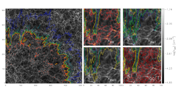
Figure 4: Slice cut of the box intercepting the region containing LOS B for a simulation with $\dot{N}_{\gamma,0}=1.36\times 10^{57}$ s^-1 at $t=10^{7}$ yrs. $n_{\textrm{gas}}$ is shown as gray color palette, while the iso-contour lines represent fronts at progressively lower ionization fraction, $x_{\textrm{HII}}={0.99996,0.99995,0.9,0.1,0.05,0.015}$, from red to blue. The box dimensions are shown in cell units (1 cell $\sim 0.05h^{-1}$ cMpc $\sim 8.4$ kpc physical), as a reference the virial radius of the halo is contained in the first four cells. The region crossed by LOS B in Figure 3, is indicated by the dashed square and zoomed-in in the four panels on the right. In these panels iso-contour lines of $x_{\textrm{HII}}$ (top left), $x_{\textrm{HeII}}$ (top right), $x_{\textrm{HeIII}}$ (bottom left) are shown with the same color scheme. The bottom right panel adopts the same color scheme to map iso-contour regions corresponding to $\log(T/{\rm K})=[4.55,4.4,4.0,3.5,3.0,2.69]$.

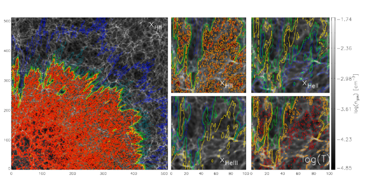
Figure 5: Slice cut of the box intercepting the region containing LOS B for a simulation with $\dot{N}_{\gamma,0}=1.36\times 10^{56}$ s^-1 at $t_{f}=10^{8}$ yrs. $n_{\textrm{gas}}$ is shown as gray color palette, while the iso-contour lines represent fronts at progressively lower ionization fraction, $x_{\textrm{HII}}={0.99996,0.99995,0.9,0.1,0.05,0.015}$, from red to blue. The box dimensions are shown in cell units (1 cell $\sim 0.05h^{-1}$ cMpc $\sim 8.4$ kpc physical), as a reference the virial radius of the halo is contained in the first four cells. The region crossed by LOS B in Figure 3, is indicated by the dashed square and zoomed-in in the four panels on the right. In these panels iso-contour lines of $x_{\textrm{HII}}$ (top left), $x_{\textrm{HeII}}$ (top right), $x_{\textrm{HeIII}}$ (bottom left) are shown with the same color scheme. The bottom right panel adopts the same color scheme to map iso-contour regions corresponding to $\log(T/{\rm K})=[4.55,4.4,4.0,3.5,3.0,2.69]$.

4.3 Statistic of ionization fronts

We now turn to a statistical analysis of the distribution of $d_{max}$, defined as the maximum distance after which the ionization fraction is found always below an assigned threshold value $x_{th}$ . Guided by the ideal cases discussed in Section 3 and Appendix B and C, we investigate the values $x_{th}=0.001,0.01,0.1,0.9$, descriptive of X-rays or UV (i.e. photons with $E_{\gamma}\leq 0.2$ keV) dominated regions found in the reference case at $t=6\times 10^{7}$ yrs.

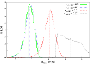
Figure 6: Percentage of LOS showing the maximum distance $d_{max}$ [physical Mpc] at which $x_{\textrm{th,HII}}$ = 0.9 (solid green line), 0.1 (dashed blue line), 0.01 (dashed-dotted red line), and 0.001 (dotted black line). Vertical lines show the average value of the distance, $\bar{d}_{max}$, with the same color conventions. The statistic refers to the simulation time $t_{i}=6\times 10^{7}$ yrs.

In Figure 6 we show the percentage of LOS for which a given $d_{max}$ value is found for a given $x_{\textrm{th,HII}}$. First note that the solid green and the dashed blue histograms are very similar and have average values of $\bar{d}_{max}=2.84$ and 2.89 Mpc. We associate these distributions with the I-front set up by the UV flux: the similar shape of the histograms and their close average values are the statistical indication of an abrupt decline of the I-front. The width of the histogram indicates instead the spread of $d_{max}$ : when $0.1<x_{\textrm{HII}}<0.9$, only $\sim 60$% of these LOS are found in 2.7 Mpc $<d_{max}<3.2$ Mpc. The tails of the distributions indicate that less than 0.1% of LOS are found in $d_{max}<2.7$ Mpc and in $d_{max}>3.2$ Mpc.

The X-rays dominated regions are instead associated with $x_{\textrm{th,HII}}=0.01$ and $x_{\textrm{th,HII}}=0.001$. The average values of their distributions are far apart from those of the UV I-front, of about 1.2 and 2.5 Mpc, i.e $\bar{d}_{max}\sim 4.1$ Mpc and $\bar{d}_{max}\sim 5.4$ Mpc, respectively. Also, note the extended width ($\approx$ 1-2 Mpc) of these low ionization regions.

To confirm the physical interpretation provided above, we now investigate the statistic of $d_{max}$ for different values of $x_{\textrm{th,HeIII}}$. In this case we expect a significant overlap in the histograms of $d_{max}$ at various ionization fractions because He$\,{\rm{\scriptstyle III}}$ does not show any extended ionization layer in the ideal tests. This statement is statistically verified in Figure 7, which has the same line and color organization of the previous one. First note the overlap of the histograms and how close their average values are (vertical lines): only $d\sim 0.7$ Mpc separate the solid green and dotted black lines; this is the statistical indication of a compact ionization front, rapidly decreasing beyond the UV dominated front ($x_{\textrm{th,HeIII}}=0.9$ at $\bar{d}_{max}\sim 2.8$ Mpc). As commented in Section 3.1.2, the low ionization rate of X-rays beyond the UV I-front is not sufficient to sustain fully ionized helium.

The same analysis (not shown here for brevity) has been performed for He$\,{\rm{\scriptstyle II}}$ and does confirm the previous comparative results.

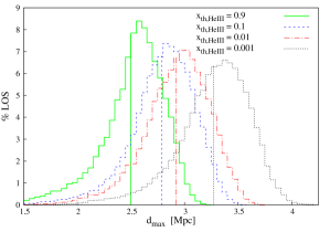
Figure 7: Percentage of LOS showing the maximum distance $d_{max}$ [physical Mpc] at which $x_{\textrm{th,HeIII}}=0.9$ (solid green line), 0.1 (dashed blue line), 0.01 (dashed-dotted red line), and 0.001 (dotted black line). Vertical lines show the average value of the distance $\bar{d}_{max}$, with same color conventions. The statistic refers to the simulation time $t_{i}=6\times 10^{7}$ yrs.

We conclude from the statistic of ionization fronts that also with realistic gas distributions X-rays create an extended, highly-fluctuating low ionization layer up to few physical Mpc, far from the emitting source.

5 CONCLUSIONS

This paper describes the impact of X-rays emitted by a high-redshift quasar on the surrounding IGM by using detailed RT simulations. The simulations are performed with the new release of the cosmological radiative transfer code CRASH4 which treats the RT problem in multi-frequency bands and self-consistently computes the gas temperature. After a brief introduction of the new code architecture, we focus on the X-ray band implementation. We first describe the various secondary ionization models implemented in CRASH4, pointing out the importance of a correct modeling of secondary ionization process. The correctness of the numerical implementation and the complications introduced by the X-ray band are first investigated in a series of idealized tests by discussing the effects of an X-ray flux on a pure hydrogen case and on a cosmological mixture of hydrogen and helium.

As a first astrophysical application, we focus on a realistic case of a quasar-like source targeting the high redshift quasar ULAS J1120+0641 (Mortlock et al., 2011). In this initial investigation we assume that the surrounding IGM is neutral when the QSO powers on. Under this hypothesis we study the detailed structure of its ionization fronts. From an accurate statistical analysis of the front along a large number of lines of sight we draw the following conclusions.

• The main ionization pattern observed in the region surrounding the QSO is determined by its UV flux, while the specific signature of X-rays consists in the creation of an extended low-ionization layer, highly sensitive to the gas over-densities surrounding the quasar halo.

• When statistically analyzed through many lines of sight, the quasar ionization front shows an average size consistent with semi-analytic estimates found in the literature, but also exhibits a non negligible scatter higher than 2 physical Mpc (i.e from $-92$% to $+26$% from the average value $R_{s}$), mainly induced by the presence of an X-ray flux in the QSO spectrum. Our statistical analysis also shows that the presence of a DLA system along a specific line of sight can significantly bias the estimate of the HII region radius, and consequently the deduced progress of reionization through proximity effect. Further investigations will be performed with the same gas distribution to assess the importance of radiative transfer effects in presence of a pre-ionized IGM, extending the findings of KK17.

• Within the observed ionization rates and the adopted DLA clustering from the hydro-dynamical simulation, we find only one LOS showing an HII region comparable with the observed one. By comparing the region created by different ionization rates and quasar lifetimes we deduce that either the ionization rate of the QSO is at least one order of magnitude lower or its bright phase is limited to $t_{f}\ll 10^{7}$ yrs to support a DLA scenario with a minimum probability.

The cosmological consequences on recombination lines, temperature history of the IGM, on the progress of helium reionization and on the detectability of the 21-cm signal will be investigated with future high-resolution reionization simulations.

Appendix A Secondary ionization models

The physics of secondary ionization was first dealt with by Spencer and Fano by providing the degradation spectrum of electrons and by calculating the energy losses induced by fast electrons (Spencer & Fano, 1954). More recent calculations account for the effects of gas ionization and metallicity: simulations in a partially ionized medium have been carried out by many authors and generally include sophisticated treatments of the micro-physical processes involving gas mixtures of H, He and eventually H2 (Spitzer & Tomasko, 1968; Habing & Goldsmith, 1971; Bergeron & Collin-Souffrin, 1973; Shull, 1979; Shull & van Steenberg, 1985; Xu & McCray, 1991; Dalgarno et al., 1999; Valdés & Ferrara, 2008). The last four implementations are briefly reviewed in the following; the interested reader can find more details in the cited literature.

Here we describe the secondary ionization models implemented in CRASH4 by briefly reviewing the main features and constraints of these models. Hereafter the quantities $f_{Q}$ and $f_{x_{i}}$ will refer to the fraction of the kinetic energy of the electrons, $E_{k}$, that goes into gas heating and collisional ionization of species $i$, respectively.

Different methods have been used to evaluate the efficiency of secondary ionization and heating, which depends on both $E_{k}$ and the ionization state of the gas, $x_{e}\equiv n_{\textrm{e}}/n_{\textrm{gas}}$, where $n_{\rm e}$ and $n_{\textrm{gas}}$ are the electron and gas number density.

Early studies employed the continuous slowing down approximation (see Pal et al. 1985 and references therein), while more recent investigations took into account the discrete nature of energy loss processes, either by solving the Spencer-Fano equation (Spencer & Fano, 1954) or by performing Monte Carlo numerical integrations (Dalgarno & Lejeune, 1971; Bergeron & Collin-Souffrin, 1973; Shull, 1979). The reliability of these results is determined largely by the accuracy of the cross sections adopted for the micro-physics of the excitation, ionization and dissociation processes.

While the efficiency of the secondary ionization process depends non-linearly on $E_{k}$ and $x_{e}$ for energies $<$100 eV, at $E_{k}>$100 eV the energy distribution of a primary electron remains approximately constant and the efficiency of the process has a linear dependence on $E_{k}$.

In gas mixtures it is generally assumed that the secondary electrons lose energy mainly in collisions with hydrogen because it normally dominates in mass. On the other hand, the presence of helium cannot be neglected because its cross sections are larger at the resonant photo-ionization potentials. When the gas is composed by H, He, H2 and metals, the process becomes increasingly more difficult to model and the definition of gas ionization fraction must be adapted to the various species releasing electrons into the gas by collisions.

In the following we will discuss in more detail the three models implemented in CRASH4.

A.1 The DG99 model

DG99 (Dalgarno et al., 1999) has an accurate treatment of many micro-physical processes including the presence of a molecular component in the gas mixture. In fact, this model simulates the slowing down of fast electrons in a partially ionized gas composed of H, He and H2. The energy deposition is calculated by a Monte Carlo scheme following the history of an electron with initial energy $E_{k}$ (Habing & Goldsmith, 1971) through the total number of excitations, ionizations and dissociations. The model includes many processes of excitation of atomic hydrogen and helium and also accounts for double ionization of helium. Although the energy loss due to electron impact excitation and ionization of He$\,{\rm{\scriptstyle II}}$ is small, the excitation of the resonance line at $30.4$ nm is accounted for because of its effects on the secondaries.

Fittings functions are given for five energy intervals in the energy range $E_{k}=30$ eV -1 keV with an accuracy, limited by the bin size, of about 2%. The fits are valid only for $10^{-6}\leq x\leq 0.1$, where $x$ is the ionization fraction. In the range of energies and ionization fraction of common validity, the DG99 numbers are in good agreement with those from SVS85, the discrepancies being mainly due to updated atomic data and a more accurate treatment of atomic processes.

Because in DG99 values of $f_{x_{i}}$ and $f_{Q}$ are provided for different compositions of the gas, in CRASH4 we have implemented tables corresponding to the five energy bins for a case of pure H, as well as for a gas composed of H and He in cosmological abundance. The energy interval is extended from 1 keV to 3 keV by linear extrapolation. Following the approach of Meijerink & Spaans (2005), for a fixed value of $E_{k}$, the tables can be extended to $x>0.1$ using the analytic functions provided in Xu & McCray (1991). For $x<10^{-6}$ we assume instead that the gas is fully neutral. The original binning in $x$ and $E_{k}$ are maintained as provided in the paper, while intermediate values are obtained by linear interpolation.

A.2 The SVS85 model

Even if outdated in the atomic coefficients, SVS85 has been adopted by all the codes participating in the Cosmological Radiative Transfer Project (Iliev et al., 2006, 2009) and it is included in CRASH4 because it results useful for code comparison and testing.

The model is based on a Monte Carlo simulation (Shull, 1979) which follows the degradation of the primary electron energy through various interactions with H and He, assumed in cosmological abundance ratio. The model treats collisional ionization of H$\,{\rm{\scriptstyle I}}$, He$\,{\rm{\scriptstyle I}}$ and He$\,{\rm{\scriptstyle II}}$, collisional excitation of the same species, and electron scattering by Coulomb collisions with thermal electrons. Interactions with He$\,{\rm{\scriptstyle III}}$ are neglected and $x_{\rm HeII}=x_{\rm HII}$ is assumed; molecules or heavy elements are not accounted for.

A series of analytic expressions for the fraction of the electron energy $E_{k}$ that goes into gas heating ($f_{Q}$), ionization of species $i$ ($f_{x_{i}}$), and line excitation of hydrogen and helium is provided as function of $E_{k}$ and gas ionization $x$. The fits are valid in the range $E_{k}=[0.1-3]$ keV and $10^{-4}\leq x\leq 0.95$ with an accuracy of $\sim$1-2%.

The SVS85 model has been implemented in CRASH4 by importing the values tabulated for $E_{k}=100$ eV and 3 keV, and by interpolating linearly within this energy range to find the energies specified in the source spectra of each CRASH4 simulation. It should be noted that the values at energies lower than $E_{k}=100$ eV are not provided by the model and they have been evaluated by linear extrapolation down to $E_{k}=30$ eV, which is a lower limit dictated by the atomic physics of collisions. Also consider that while the interpolation in the range 100 eV-3 keV is justified because of the linear dependence of $f_{x_{i}}$ and $f_{Q}$ on $E_{k}$ in this energy range, the extrapolation at lower energies is arbitrary and not documented in literature covering the numerical implementation of other codes.

For each electron energy, the binning in $x$ provided by the SVS85 model is maintained, while intermediate values are obtained by linear interpolation. We assume that for $x>0.95$ the fractions are the same as for $x=0.95$, while we linearly extrapolate the values of $f_{x_{i}}$ and $f_{Q}$ at $x=10^{-4}$ down to $10^{-6}$ (the minimum value of validity for the DG99 model) and assume that $x=0$ for even lower ionization levels.

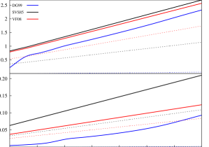
Figure 8: Average number of collisional ionizations of H$\,{\rm{\scriptstyle I}}$ (top panel) and He$\,{\rm{\scriptstyle I}}$ (bottom panel) as a function of the electron energy $E_{k}$ in the non-linear regime $E_{k}<100$ eV, with $x=0.1$ (dashed lines) and $x=10^{-4}$ (solid lines). The DG99, SVS85 and VF08 models are represented by blue, black and red lines, respectively.

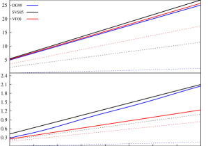
Figure 9: Average number of collisional ionizations of H$\,{\rm{\scriptstyle I}}$ (top panel) and He$\,{\rm{\scriptstyle I}}$ (bottom panel) as a function of the electron energy $E_{k}$ in the non-linear regime $E_{k}>100$ eV, with $x=0.1$ (dashed lines) and $x=10^{-4}$ (solid lines). The DG99, SVS85 and VF08 models are represented by blue, black and red lines, respectively.

A.3 VF08 model

The VF08 model provides one of the most advanced and updated implementations of atomic data in the literature and fitting trends valid for $E_{k}>3$ keV. The adoption of VF08 will allow then a future integration of secondary effects from the hard X-ray and gamma spectral bands (Valdés et al., 2010). Following the method used by SVS85, this model includes the most recent atomic data, accurate cross sections for collisional ionization and excitations from electron impacts, electron-electron collisions, free-free interactions and gas recombinations. Together with the inclusion of the generally neglected two-photon forbidden transition $2s\rightarrow 1s$, processes producing continuum photons (i.e. gas recombinations, Bremsstrahlung free-free and ion-electron interactions) are also accounted for. As SVS85, they assume a gas made of H and He in cosmological proportions and $x_{\rm HeII}=x_{\rm HII}$, neglecting doubly ionized helium. Values for the fraction of energy going into photons with energy below 10.2 eV are provided as well.

Fitting functions for $f_{x_{i}}$ and $f_{Q}$ are provided in the range $E_{k}$=[3-10] keV, with an accuracy better than 3.5%. The validity range in ionization fraction is $10^{-4}\leq x\leq 0.99$. For $x<0.1$ the functions are very similar to those provided by SVS85, while differences as large as 30% are found for higher ionization fractions.

The inclusion of VF08 in CRASH4 has been done as the one of SVS85, i.e. by importing the values tabulated for $E_{k}=10$ keV, and evaluating the values at lower energies by linear extrapolation down to $E_{k}=30$ eV. The extension of the tables to a wider range of ionization fraction has been done as for SVS85.

In the paragraphs below we summarise the behaviour of the three models by showing the average number of collisional ionizations, $N_{s,i}$, as function of the photo-electron energy $E_{k}$ in the non-linear (Figure A1) and linear regime (Figure A2). In both figures we only show the ionizations of H$\,{\rm{\scriptstyle I}}$ and He$\,{\rm{\scriptstyle I}}$ because only the DG99 model provides values for He$\,{\rm{\scriptstyle II}}$. We show curves for $x=10^{-4}$ and 0.1, which are the minimum and maximum ionization fraction shared by the three models. For $E_{k}<100$ eV DG99 is the only accurate model, while the curves from SVS85 and VF08 are obtained by linear extrapolation of results at $E_{k}=100$ eV and 3 keV, respectively. From Figure A1 it is clear that the number of collisional ionizations is largely overestimated when a linear extrapolation is applied, and that the discrepancy with the DG99 model increases with the ionization fraction. In fact, while for $x\lower 2.15277pt\hbox{$\;\buildrel>\over{\sim}\;$}0.1$ hardly any ionization occurs in the DG99 model, this is not the case for SVS85 and VF08. The above considerations apply both for H$\,{\rm{\scriptstyle I}}$ and He$\,{\rm{\scriptstyle I}}$. Substantial differences exist also in the linear regime shown in Figure A2. While in a quasi-neutral medium (solid lines) the agreement between the models is extremely good (at least for H$\,{\rm{\scriptstyle I}}$), it rapidly worsens with increasing ionization fractions, with SVS85 and VF08 finding larger $N_{\rm s,HI}$ and $N_{\rm s,HeI}$, as in the non linear regime.

Appendix B Impact of secondary ionization models on H$\,{\rm{\scriptstyle II}}$ regions

To understand how the choice of a specific secondary ionization model impacts the final properties of the H$\,{\rm{\scriptstyle II}}$ regions (see Figure 2), we ran the same test of Section 3.2 by adopting the SVS85 and VF08 models. In addition to the standard ionization rate $\dot{N}_{\gamma,0}=1.36\times 10^{56}$ photons s^-1 we also considered the case with $\dot{N}_{\gamma,1}=1.36\times 10^{57}$ photons s^-1.

The results of this comparison are summarized in Figure B1 for a case in which the contribution from X-rays and secondary ionization is included. First note that for the simple configuration of this test the results provided by SVS85 and VF08 are indistinguishable in the case with $\dot{N}_{\gamma,0}$, while few small differences in the hydrogen and helium profiles are found in the remaining cases.

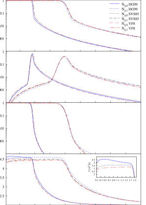
Figure 10: Radial profiles of the Strömgren sphere created in a cosmological mixture of H and He at the simulation time $t_{i}=6\times 10^{7}$ yrs. The distance $d$ from the source is shown in physical Mpc. In all the panels the profiles are obtained using the model: DG99 (blue lines), SVS85 (black) and VF08 (red). For each simulation set two cases are considered: $\dot{N}_{\gamma,0}=1.36\times 10^{56}$ photons s^-1 and $\dot{N}_{\gamma,1}=1.36\times 10^{57}$ photons s^-1. From the top to the bottom the panels refer to the profiles of $x_{\textrm{HII}}$, $x_{\textrm{HeII}}$, $x_{\textrm{HeIII}}$ and log$(T)$ [K]. The small box in the bottom panel shows a zoom of the gas temperature (in linear scale of $10^{4}$ K) in the fully ionized region 0.1 Mpc $<d<2.0$ Mpc, physical.

Second, while a discrepancy is found between DG99 and the other models and it increases at higher ionization rates, DG99 always predicts a radius of the I-front smaller by 13%. These differences are due to the different behavior of the models in the limit $x_{e}\rightarrow 0$ (see Appendix A). Other differences in the $x_{\rm HeII}$ and $x_{\rm HeIII}$ profiles are also present although less evident.

The highest discrepancy though is observed in the temperature (bottom panel and small box inside it), which is systematically higher in the DG99 model. These differences are due not only to the linear extrapolation of models SVS85 and VF08 at energies below their valodity limit, but in the way the heating mechanism is modelled. SVS85 and VF08 tend in fact to over-estimate the ionization reducing the contribution to the photo-heating (see Figures A1 and A2 in Appendix A) but also to distribute more energy to excitations instead of gas photo-heating.

Appendix C Effects of initial conditions

Here we show a series of ideal tests repeated in a range of gas number densities, and non neutral initial conditions. The reference secondary ionization model adopted for runs with varying number density is DG99, while VF08 is adopted for tests with varying initial ionization fractions to allow a direct comparison with the results in Appendix B and Section 4.

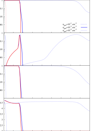
Figure 11: Radial profiles of the Strömgren sphere created by a QSO-like source in cosmological mixture of H and He by adopting the DG99 model and different values of the gas number density: $n_{gas}=10^{-1}$ cm^-3 (dashed lines), $10^{-3}$ cm^-3 (solid), and $10^{-5}$ cm^-3 (dotted). The lines refer to the simulation time in all the configurations $t_{i}=6\times 10^{7}$ yrs. The distance $d$ from the source is shown in physical Mpc. In all the panels the profiles referring to the (UV+X) case are represented as blue lines. Only for the case $n_{gas}=10^{-3}$ cm^-3 we show the profile with UV radiation only(red lines). From the top to the bottom the panels refer to the profiles of $x_{\textrm{HII}}$, $x_{\textrm{HeII}}$, $x_{\textrm{HeIII}}$ and log$(T)$ [K].

Here we show ideal tests adopting the same parameters as in Section 4 but for the gas density which is set up as uniform in space. As always the convergence of the solutions has been verified with an identical simulation increasing the number of packets by one order of magnitude. We varied the gas number density in the range $n_{gas}\in[10^{-1},10^{-5}]$ cm^-3; some representative profiles are shown in Figure C1 with the same color convention used in Section 3. Here different line-styles correspond to different values of the gas number density: $n_{gas}=10^{-1}$ cm^-3 in dashed, $n_{gas}=10^{-3}$ cm^-3 in solid, and finally $n_{gas}=10^{-5}$ cm^-3 in dotted. As always we show the profiles in physical distance $d$.

First note how the profiles of the Strömgren spheres are really sensitive to the gas number density both in the I-front positions and the extended shells at low ionization found in the reference case (solid lines). For example in the top panel we show how the hydrogen I-fronts of the spheres change from $d\sim 0.15$ Mpc to $d\sim 0.95$ Mpc, and finally $d>3.7$ Mpc, when the gas number density changes by one order of magnitude. The external shell increases its extension accordingly (compare the blue lines) and escapes the domain boundaries when $n_{gas}=10^{-5}$ cm^-3. By comparing the blue and red lines we note also how the X-rays band becomes progressively more effective in creating a diffuse profile when the gas number density decreases. Similar considerations can be applied at the ions of helium in the middle and bottom panels. In particular note how easy it is to maintain the helium fully ionized at large distances when the number density reached $n_{gas}=10^{-5}$ cm^-3.

The temperature profiles are impacted as well, as shown in the bottom panel. The entire cube is set up at photo-ionization temperature in the lowest density case while in the case $n_{gas}=10^{-3}$ cm^-3 the gas temperature is maintained at $T>10^{3}$ K at distances larger than $d\sim 0.9$ physical Mpc only by the X-rays contribution. The column density created by $n_{gas}=10^{-1}$ cm^-3 on the other hand is sufficient to completely stop the soft X-ray flux by 0.15 Mpc from the QSO source.

In the paragraphs below we study the dependence of our results when an initial ionization $x_{0}$ of the gas is assumed. For this test we adopt the gas number density of the reference case $n_{gas}=9.59\times 10^{-5}$ cm^-3 and assume an initial ionization $x_{0,\textrm{HII}}=x_{0,\textrm{HeII}}=x_{0}=$0.01, 0.1 and 0.5, while $x_{0,\textrm{HeIII}}=0$.

When a pre-ionization $x_{0}<0.1$ is set up, all the species rapidly increase their ionization in the external, low ionization region ($d>1.5$ Mpc), as evident by comparing all the lines with the dashed-dotted one. This is because an initial ionization decreases the gas optical depth in both H$\,{\rm{\scriptstyle II}}$ and He$\,{\rm{\scriptstyle II}}$ and then the profiles of He$\,{\rm{\scriptstyle III}}$ change as well. Longer tails in the temperature profiles are also created (see bottom panel) by inducing gas temperatures higher than $T=1000$ K at $d>2.0$ Mpc.

Smaller effects are found instead on the ionization I-fronts of the Strömgren spheres which show a noticeable shift only for $x_{0}>0.1$. Also note that a pre-ionization condition has a substantial impact on the temperature of the fully ionized gas which reaches a lower photo-ionization equilibrium temperature (compare dotted curve with dashed-dotted in the bottom panel).

As final remark, we point out that tests performed by mixing initial ionization $x_{0}\sim 0.01$ and temperatures $T_{0}\sim 10^{3}$ K have been performed as well during the test of CRASH4 without finding remarkable differences with the results shown in this section.

Appendix D Infinite speed of light effects on time evolution

Here we repeat Tests 3.1 and 3.2 with longer simulation duration to capture the late evolution of the HII region. To find the equilibrium configuration in a gas of $n_{\textrm{gas}}=9.59\times 10^{-5}$ cm^-3 we should set up a final time $t_{f}=4\times t_{rec}\sim 4\times 10^{9}$ yrs, as prescribed in a similar test of the Cosmological Radiative Transfer Comparison Project (Iliev et al., 2006). Note that while $t_{f}\sim 10^{9}$ yrs is still consistent with extreme low-redshift QSO lifetimes (Martini & Weinberg, 2001), our simulation would reach $z\sim 1.34$ when the assumption that the bubble tail expands in a neutral gas (i.e. isolated QSO) is unrealistic. We have thus chosen to end the simulation at $t_{f}=10^{8}$ yrs, which corresponds to $z\sim 6.45$. This time is sufficiently long to follow the late evolution of the tails in our idealized set-up. The box size is $110h^{-1}$ Mpc comoving but with the same grid resolution as in Section 3.1.

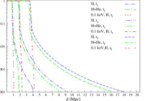
Figure 12: Radial profiles of $x_{\textrm{HII}}$ of the Strömgren sphere created in a gas made of neutral atomic hydrogen only (blue/red lines) and H+He (green) at different simulation times: $t_{i}=2\times 10^{6}$ yrs, $t_{s}=2\times 10^{7}$ yrs, $t_{f}=10^{8}$ yrs. The secondary ionization model adopted in the simulation is DG99. The distance $d$ from the source is shown in physical Mpc. Blue and green lines refer to a spectrum cut at $E_{\textrm{max}}=3$ keV, while red lines refer to $E_{\textrm{max}}=0.1$ keV.

$t$ [yrs]	$z$	$R_{c}$ [Mpc]	$R_{s}$ [Mpc]	$v_{f,c}$ [$c$]	$d_{\textrm{max},0.001}$ [Mpc](H/H+He)	$d_{\textrm{max},0.0001}$ [Mpc](H/H+He)	$d_{c,\textrm{vac}}$ [Mpc]
$2\times 10^{6}$	$7.07$	$0.850$	$0.891$	$1.24$	2.40/1.77	4.10/1.88	0.6
$4\times 10^{6}$	$7.06$	$1.072$	$1.123$	$0.78$	3.0/2.0	4.44/2.52	1.23
$6\times 10^{6}$	$7.04$	$1.259$	$1.285$	$0.61$	3.45/2.45	5.34/4.52	1.85
$8\times 10^{6}$	$7.03$	$1.373$	$1.415$	$0.51$	3.75/2.93	6.32/5.50	2.45
$10^{7}$	$7.01$	$1.487$	$1.524$	$0.43$	4.02/3.31	7.04/6.22	3.07
$2\times 10^{7}$	$6.94$	$1.912$	$1.920$	$0.28$	4.95/4.43	9.46/8.45	6.14
$4\times 10^{7}$	$6.82$	$2.478$	$2.419$	$0.18$	6.45/5.80	12.40/11.14	12.27
$6\times 10^{7}$	$6.69$	$2.906$	$2.769$	$0.14$	7.56/6.83	14.58/13.11	18.50
$10^{8}$	$6.45$	$3.64$	$3.283$	$0.11$	9.41/8.49	18.14/16.30	30.70

Table 1: Time evolution of the $x_{\textrm{HII}}$ profiles. $t$ is the simulation time in years, $z$ is the redshift, $R_{c}$ is the I-front position computed by CRASH4 and $R_{s}$ is the I-front of the semi-analytic estimate in formula (3), both in proper Mpc. $v_{f,c}$ is the I-front speed computed from $R_{c}$, in units of $c\sim 3\times 10^{10}$ cm s^-1. $d_{\textrm{max},0.001}$ and $d_{\textrm{max},0.0001}$ are the maximum extension of the $x_{\textrm{HII}}$ profiles at $x_{\textrm{HII}}>0.001$ and $x_{\textrm{HII}}>0.0001$, respectively. The H/H+He nomenclature refers to the H only and H+He cases. As a reference, the last column shows the maximum distance traveled by light in vacuum at fixed time ($d_{c,\textrm{vac}}$).

Figure D1 shows the spherically averaged radial profiles of $x_{\textrm{HII}}$ at different times for both 0.1 keV and 3 keV cases; by comparing them the contribution of X-rays to the tails becomes evident. The more realistic case in which helium is included is also shown by green lines. Table D1 complements Figure D1 by providing more details on the fronts obtained with the cosmic web discussed in Section 4 at early and late times: $R_{c}$ is the value of the I-front position computed by CRASH4, $R_{s}$ the value inferred by equation (3) and $v_{f,c}$ is the front speed computed for $R_{c}$, in units of physical speed of light $c\sim 3\times 10^{10}$ cm s^-1. The maximum tail extension at assigned time and ionization fraction ($d_{max,x_{\textrm{HII}}}$) is computed for $x_{\textrm{HII}}=0.001,0.0001$ and can be compared with the maximum distance traveled by light in vacuum ($d_{c,\textrm{vac}}$). Note that $x_{\textrm{HII}}=0.0001$ is the lowest Monte Carlo convergent value found in our simulation by sampling the source with $2\times 10^{8}$ photon packets.

The extension of the tails is overestimated at short times as they are present beyond the maximum distance traveled by radiation in vacuum. This error is due to the infinite speed of light approximation which creates an excess of high energy photons beyond the I-front and induces an early growth of the external regions. As shown in the table, this effect becomes progressively less evident in time and disappears at $t=6\times 10^{7}$ yrs. The effective impact on the time evolution of the tail cannot be assessed with a single rule of thumb, as it depends both on the source properties (e.g. it is higher in the early evolution of extremely bright sources), gas number density and the efficiency of secondary electrons. In conclusion, its impact has to be verified depending on the problem at hand.

References

- Allen et al. (2008) Allen M. G., Groves B. A., Dopita M. A., Sutherland R. S., Kewley L. J., 2008, \hrefhttp://dx.doi.org/10.1086/589652 ApJS, \hrefhttp://adsabs.harvard.edu/abs/2008ApJS..178…20A 178, 20
- Bañados et al. (2018) Bañados E., et al., 2018, \hrefhttp://dx.doi.org/10.1038/nature25180 NATURE, \hrefhttp://adsabs.harvard.edu/abs/2018Natur.553..473B 553, 473
- Badnell et al. (2005) Badnell N. R., Bautista M. A., Butler K., Delahaye F., Mendoza C., Palmeri P., Zeippen C. J., Seaton M. J., 2005, \hrefhttp://dx.doi.org/10.1111/j.1365-2966.2005.08991.x MNRAS, \hrefhttp://adsabs.harvard.edu/abs/2005MNRAS.360..458B 360, 458
- Baek et al. (2010) Baek S., Semelin B., Di Matteo P., Revaz Y., Combes F., 2010, \hrefhttp://dx.doi.org/10.1051/0004-6361/201014347 AAP, \hrefhttp://adsabs.harvard.edu/abs/2010A
- Bergeron & Collin-Souffrin (1973) Bergeron J., Collin-Souffrin S., 1973, AAP, \hrefhttp://adsabs.harvard.edu/abs/1973A
- Berrington et al. (1974) Berrington K. A., Burke P. G., Chang J. J., Chivers A. T., Robb W. D., Taylor K. T., 1974, \hrefhttp://dx.doi.org/10.1016/0010-4655(74)90096-4 Computer Physics Communications, \hrefhttp://adsabs.harvard.edu/abs/1974CoPhC…8..149B 8, 149
- Berrington et al. (1987) Berrington K. A., Burke P. G., Butler K., Seaton M. J., Storey P. J., Taylor K. T., Yan Y., 1987, \hrefhttp://dx.doi.org/10.1088/0022-3700/20/23/027 Journal of Physics B Atomic Molecular Physics, \hrefhttp://adsabs.harvard.edu/abs/1987JPhB…20.6379B 20, 6379
- Bolton et al. (2011) Bolton J. S., Haehnelt M. G., Warren S. J., Hewett P. C., Mortlock D. J., Venemans B. P., McMahon R. G., Simpson C., 2011, \hrefhttp://dx.doi.org/10.1111/j.1745-3933.2011.01100.x MNRAS, \hrefhttp://adsabs.harvard.edu/abs/2011MNRAS.416L..70B 416, L70
- Bryan et al. (2014) Bryan G. L., et al., 2014, \hrefhttp://dx.doi.org/10.1088/0067-0049/211/2/19 ApJS, \hrefhttp://adsabs.harvard.edu/abs/2014ApJS..211…19B 211, 19
- Burke et al. (2006) Burke P. G., Noble C. J., Burke V. M., 2006, \hrefhttp://dx.doi.org/10.1016/S1049-250X(06)54005-4 Advances in Atomic Molecular and Optical Physics, \hrefhttp://adsabs.harvard.edu/abs/2006AAMOP..54..237B 54, 237
- Cen & Haiman (2000) Cen R., Haiman Z., 2000, \hrefhttp://dx.doi.org/10.1086/312937 ApJL, \hrefhttp://adsabs.harvard.edu/abs/2000ApJ…542L..75C 542, L75
- Ciardi & Madau (2003) Ciardi B., Madau P., 2003, \hrefhttp://dx.doi.org/10.1086/377634 ApJ, \hrefhttp://adsabs.harvard.edu/abs/2003ApJ…596….1C 596, 1
- Ciardi et al. (2001) Ciardi B., Ferrara A., Marri S., Raimondo G., 2001, \hrefhttp://dx.doi.org/10.1046/j.1365-8711.2001.04316.x MNRAS, \hrefhttp://adsabs.harvard.edu/abs/2001MNRAS.324..381C 324, 381
- Cunto et al. (1993) Cunto W., Mendoza C., Ochsenbein F., Zeippen C. J., 1993, AAP, \hrefhttp://adsabs.harvard.edu/abs/1993A
- Dalgarno & Lejeune (1971) Dalgarno A., Lejeune G., 1971, \hrefhttp://dx.doi.org/10.1016/0032-0633(71)90126-7 PLANSS, \hrefhttp://adsabs.harvard.edu/abs/1971P
- Dalgarno et al. (1963) Dalgarno A., McElroy M. B., Moffett R. J., 1963, \hrefhttp://dx.doi.org/10.1016/0032-0633(63)90071-0 PLANSS, \hrefhttp://adsabs.harvard.edu/abs/1963P
- Dalgarno et al. (1999) Dalgarno A., Yan M., Liu W., 1999, \hrefhttp://dx.doi.org/10.1086/313267 ApJS, \hrefhttp://adsabs.harvard.edu/abs/1999ApJS..125..237D 125, 237
- Das et al. (2017) Das A., Mesinger A., Pallottini A., Ferrara A., Wise J. H., 2017, \hrefhttp://dx.doi.org/10.1093/mnras/stx943 MNRAS, \hrefhttp://adsabs.harvard.edu/abs/2017MNRAS.469.1166D 469, 1166
- Eide et al. (2018) Eide M. B., Graziani L., Ciardi B., Feng Y., Kakiichi K., Di Matteo T., 2018, \hrefhttp://dx.doi.org/10.1093/mnras/sty272 MNRAS, \hrefhttp://adsabs.harvard.edu/abs/2018MNRAS.476.1174E 476, 1174
- Ercolano et al. (2008) Ercolano B., Young P. R., Drake J. J., Raymond J. C., 2008, \hrefhttp://dx.doi.org/10.1086/524378 ApJS, \hrefhttp://adsabs.harvard.edu/abs/2008ApJS..175..534E 175, 534
- Evoli et al. (2012) Evoli C., Valdés M., Ferrara A., Yoshida N., 2012, \hrefhttp://dx.doi.org/10.1111/j.1365-2966.2012.20624.x MNRAS, \hrefhttp://adsabs.harvard.edu/abs/2012MNRAS.422..420E 422, 420
- Ewall-Wice et al. (2016) Ewall-Wice A., et al., 2016, \hrefhttp://dx.doi.org/10.1093/mnras/stw1022 MNRAS, \hrefhttp://adsabs.harvard.edu/abs/2016MNRAS.460.4320E 460, 4320
- Ferland et al. (1998) Ferland G. J., Korista K. T., Verner D. A., Ferguson J. W., Kingdon J. B., Verner E. M., 1998, \hrefhttp://dx.doi.org/10.1086/316190 PASP, \hrefhttp://adsabs.harvard.edu/abs/1998PASP..110..761F 110, 761
- Ferland et al. (2013) Ferland G. J., et al., 2013, RMXAA, \hrefhttp://adsabs.harvard.edu/abs/2013RMxAA..49..137F 49, 137
- Fialkov et al. (2014) Fialkov A., Barkana R., Visbal E., 2014, \hrefhttp://dx.doi.org/10.1038/nature12999 NATURE, \hrefhttp://adsabs.harvard.edu/abs/2014Natur.506..197F 506, 197
- Friedrich et al. (2012) Friedrich M. M., Mellema G., Iliev I. T., Shapiro P. R., 2012, \hrefhttp://dx.doi.org/10.1111/j.1365-2966.2012.20449.x MNRAS, \hrefhttp://adsabs.harvard.edu/abs/2012MNRAS.421.2232F 421, 2232
- Furlanetto et al. (2006) Furlanetto S. R., Oh S. P., Briggs F. H., 2006, \hrefhttp://dx.doi.org/10.1016/j.physrep.2006.08.002 Physrep, \hrefhttp://adsabs.harvard.edu/abs/2006PhR…433..181F 433, 181
- Glover & Brand (2003) Glover S. C. O., Brand P. W. J. L., 2003, \hrefhttp://dx.doi.org/10.1046/j.1365-8711.2003.06311.x MNRAS, \hrefhttp://adsabs.harvard.edu/abs/2003MNRAS.340..210G 340, 210
- Graziani et al. (2013) Graziani L., Maselli A., Ciardi B., 2013, \hrefhttp://dx.doi.org/10.1093/mnras/stt206 MNRAS, \hrefhttp://adsabs.harvard.edu/abs/2013MNRAS.431..722G 431, 722
- Graziani et al. (2015) Graziani L., Salvadori S., Schneider R., Kawata D., de Bennassuti M., Maselli A., 2015, \hrefhttp://dx.doi.org/10.1093/mnras/stv494 MNRAS, \hrefhttp://adsabs.harvard.edu/abs/2015MNRAS.449.3137G 449, 3137
- Graziani et al. (2017) Graziani L., de Bennassuti M., Schneider R., Kawata D., Salvadori S., 2017, \hrefhttp://dx.doi.org/10.1093/mnras/stx900 MNRAS, \hrefhttp://adsabs.harvard.edu/abs/2017MNRAS.469.1101G 469, 1101
- Habing & Goldsmith (1971) Habing H. J., Goldsmith D. W., 1971, \hrefhttp://dx.doi.org/10.1086/150979 ApJ, \hrefhttp://adsabs.harvard.edu/abs/1971ApJ…166..525H 166, 525
- Hariharan et al. (2017) Hariharan N., Graziani L., Ciardi B., Miniati F., Bungartz H.-J., 2017, \hrefhttp://dx.doi.org/10.1093/mnras/stx162 MNRAS, \hrefhttp://adsabs.harvard.edu/abs/2017MNRAS.467.2458H 467, 2458
- Iliev et al. (2006) Iliev I. T., et al., 2006, \hrefhttp://dx.doi.org/10.1111/j.1365-2966.2006.10775.x MNRAS, \hrefhttp://adsabs.harvard.edu/abs/2006MNRAS.371.1057I 371, 1057
- Iliev et al. (2009) Iliev I. T., et al., 2009, \hrefhttp://dx.doi.org/10.1111/j.1365-2966.2009.15558.x MNRAS, \hrefhttp://adsabs.harvard.edu/abs/2009MNRAS.400.1283I 400, 1283
- Jeon et al. (2014) Jeon M., Pawlik A. H., Bromm V., Milosavljević M., 2014, \hrefhttp://dx.doi.org/10.1093/mnras/stu444 \mnras, \hrefhttp://adsabs.harvard.edu/abs/2014MNRAS.440.3778J 440, 3778
- Kakiichi et al. (2017) Kakiichi K., Graziani L., Ciardi B., Meiksin A., Compostella M., Eide M. B., Zaroubi S., 2017, \hrefhttp://dx.doi.org/10.1093/mnras/stx603 MNRAS, \hrefhttp://adsabs.harvard.edu/abs/2017MNRAS.468.3718K 468, 3718
- Kallman (1984) Kallman T. R., 1984, \hrefhttp://dx.doi.org/10.1086/161994 ApJ, \hrefhttp://adsabs.harvard.edu/abs/1984ApJ…280..269K 280, 269
- Kallman (2010) Kallman T. R., 2010, \hrefhttp://dx.doi.org/10.1007/s11214-010-9711-6 SSR, \hrefhttp://adsabs.harvard.edu/abs/2010SSRv..157..177K 157, 177
- Keating et al. (2015) Keating L. C., Haehnelt M. G., Cantalupo S., Puchwein E., 2015, \hrefhttp://dx.doi.org/10.1093/mnras/stv2020 MNRAS, \hrefhttp://adsabs.harvard.edu/abs/2015MNRAS.454..681K 454, 681
- Kern et al. (2017) Kern N. S., Liu A., Parsons A. R., Mesinger A., Greig B., 2017, \hrefhttp://dx.doi.org/10.3847/1538-4357/aa8bb4 \apj, \hrefhttp://adsabs.harvard.edu/abs/2017ApJ…848…23K 848, 23
- Khrykin et al. (2016) Khrykin I. S., Hennawi J. F., McQuinn M., Worseck G., 2016, \hrefhttp://dx.doi.org/10.3847/0004-637X/824/2/133 ApJ, \hrefhttp://adsabs.harvard.edu/abs/2016ApJ…824..133K 824, 133
- Lee et al. (2016) Lee K.-Y., Mellema G., Lundqvist P., 2016, \hrefhttp://dx.doi.org/10.1093/mnras/stv2556 MNRAS, \hrefhttp://adsabs.harvard.edu/abs/2016MNRAS.455.4406L 455, 4406
- Madau & Fragos (2017) Madau P., Fragos T., 2017, \hrefhttp://dx.doi.org/10.3847/1538-4357/aa6af9 ApJ, \hrefhttp://adsabs.harvard.edu/abs/2017ApJ…840…39M 840, 39
- Madau & Rees (2000) Madau P., Rees M. J., 2000, \hrefhttp://dx.doi.org/10.1086/312934 ApJL, \hrefhttp://adsabs.harvard.edu/abs/2000ApJ…542L..69M 542, L69
- Madau et al. (1997) Madau P., Meiksin A., Rees M. J., 1997, \hrefhttp://dx.doi.org/10.1086/303549 ApJ, \hrefhttp://adsabs.harvard.edu/abs/1997ApJ…475..429M 475, 429
- Martini & Weinberg (2001) Martini P., Weinberg D. H., 2001, \hrefhttp://dx.doi.org/10.1086/318331 ApJ, \hrefhttp://adsabs.harvard.edu/abs/2001ApJ…547…12M 547, 12
- Maselli et al. (2003) Maselli A., Ferrara A., Ciardi B., 2003, \hrefhttp://dx.doi.org/10.1046/j.1365-8711.2003.06979.x MNRAS, \hrefhttp://adsabs.harvard.edu/abs/2003MNRAS.345..379M 345, 379
- Maselli et al. (2004) Maselli A., Ferrara A., Bruscoli M., Marri S., Schneider R., 2004, \hrefhttp://dx.doi.org/10.1111/j.1365-2966.2004.07810.x MNRAS, \hrefhttp://adsabs.harvard.edu/abs/2004MNRAS.350L..21M 350, L21
- Maselli et al. (2007) Maselli A., Gallerani S., Ferrara A., Choudhury T. R., 2007, \hrefhttp://dx.doi.org/10.1111/j.1745-3933.2007.00283.x MNRAS, \hrefhttp://adsabs.harvard.edu/abs/2007MNRAS.376L..34M 376, L34
- Maselli et al. (2009a) Maselli A., Ciardi B., Kanekar A., 2009a, \hrefhttp://dx.doi.org/10.1111/j.1365-2966.2008.14197.x MNRAS, \hrefhttp://adsabs.harvard.edu/abs/2009MNRAS.393..171M 393, 171
- Maselli et al. (2009b) Maselli A., Ferrara A., Gallerani S., 2009b, \hrefhttp://dx.doi.org/10.1111/j.1365-2966.2009.14699.x MNRAS, \hrefhttp://adsabs.harvard.edu/abs/2009MNRAS.395.1925M 395, 1925
- Meijerink & Spaans (2005) Meijerink R., Spaans M., 2005, \hrefhttp://dx.doi.org/10.1051/0004-6361:20042398 AAP, \hrefhttp://adsabs.harvard.edu/abs/2005A
- Meiksin et al. (2017) Meiksin A., Khochfar S., Paardekooper J.-P., Dalla Vecchia C., Kohn S., 2017, \hrefhttp://dx.doi.org/10.1093/mnras/stx1857 \mnras, \hrefhttp://adsabs.harvard.edu/abs/2017MNRAS.471.3632M 471, 3632
- Mesinger et al. (2011) Mesinger A., Furlanetto S., Cen R., 2011, \hrefhttp://dx.doi.org/10.1111/j.1365-2966.2010.17731.x MNRAS, \hrefhttp://adsabs.harvard.edu/abs/2011MNRAS.411..955M 411, 955
- Mesinger et al. (2013) Mesinger A., Ferrara A., Spiegel D. S., 2013, \hrefhttp://dx.doi.org/10.1093/mnras/stt198 MNRAS, \hrefhttp://adsabs.harvard.edu/abs/2013MNRAS.431..621M 431, 621
- Mortlock et al. (2011) Mortlock D. J., et al., 2011, \hrefhttp://dx.doi.org/10.1038/nature10159 NATURE, \hrefhttp://adsabs.harvard.edu/abs/2011Natur.474..616M 474, 616
- Oh (2001) Oh S. P., 2001, \hrefhttp://dx.doi.org/10.1086/320957 ApJ, \hrefhttp://adsabs.harvard.edu/abs/2001ApJ…553..499O 553, 499
- Pacucci et al. (2014) Pacucci F., Mesinger A., Mineo S., Ferrara A., 2014, \hrefhttp://dx.doi.org/10.1093/mnras/stu1240 MNRAS, \hrefhttp://adsabs.harvard.edu/abs/2014MNRAS.443..678P 443, 678
- Pal et al. (1985) Pal P. B., Gupta S. K., Varshney V. P., Gupta D. K., 1985, \hrefhttp://dx.doi.org/10.1143/JJAP.24.1070 Japanese Journal of Applied Physics, \hrefhttp://adsabs.harvard.edu/abs/1985JaJAP..24.1070P 24, 1070
- Piconcelli et al. (2005) Piconcelli E., Jimenez-Bailón E., Guainazzi M., Schartel N., Rodríguez-Pascual P. M., Santos-Lleó M., 2005, \hrefhttp://dx.doi.org/10.1051/0004-6361:20041621 AAP, \hrefhttp://adsabs.harvard.edu/abs/2005A
- Pierleoni et al. (2009) Pierleoni M., Maselli A., Ciardi B., 2009, \hrefhttp://dx.doi.org/10.1111/j.1365-2966.2008.13874.x MNRAS, \hrefhttp://adsabs.harvard.edu/abs/2009MNRAS.393..872P 393, 872
- Pritchard & Furlanetto (2007) Pritchard J. R., Furlanetto S. R., 2007, \hrefhttp://dx.doi.org/10.1111/j.1365-2966.2007.11519.x MNRAS, \hrefhttp://adsabs.harvard.edu/abs/2007MNRAS.376.1680P 376, 1680
- Pritchard & Loeb (2012) Pritchard J. R., Loeb A., 2012, \hrefhttp://dx.doi.org/10.1088/0034-4885/75/8/086901 Reports on Progress in Physics, \hrefhttp://adsabs.harvard.edu/abs/2012RPPh…75h6901P 75, 086901
- Ricotti et al. (2002) Ricotti M., Gnedin N. Y., Shull J. M., 2002, \hrefhttp://dx.doi.org/10.1086/341255 ApJ, \hrefhttp://adsabs.harvard.edu/abs/2002ApJ…575…33R 575, 33
- Ripamonti et al. (2008) Ripamonti E., Mapelli M., Zaroubi S., 2008, \hrefhttp://dx.doi.org/10.1111/j.1365-2966.2008.13104.x MNRAS, \hrefhttp://adsabs.harvard.edu/abs/2008MNRAS.387..158R 387, 158
- Ross et al. (2017) Ross H. E., Dixon K. L., Iliev I. T., Mellema G., 2017, \hrefhttp://dx.doi.org/10.1093/mnras/stx649 MNRAS, \hrefhttp://adsabs.harvard.edu/abs/2017MNRAS.468.3785R 468, 3785
- Seaton (2005) Seaton M. J., 2005, \hrefhttp://dx.doi.org/10.1111/j.1365-2966.2005.00019.x MNRAS, \hrefhttp://adsabs.harvard.edu/abs/2005MNRAS.362L…1S 362, L1
- Seaton et al. (1992) Seaton M. J., Zeippen C. J., Tully J. A., Pradhan A. K., Mendoza C., Hibbert A., Berrington K. A., 1992, RMXAA, \hrefhttp://adsabs.harvard.edu/abs/1992RMxAA..23…19S 23, 19
- Semelin et al. (2017) Semelin B., Eames E., Bolgar F., Caillat M., 2017, \hrefhttp://dx.doi.org/10.1093/mnras/stx2274 MNRAS, \hrefhttp://adsabs.harvard.edu/abs/2017MNRAS.472.4508S 472, 4508
- Shull (1979) Shull J. M., 1979, \hrefhttp://dx.doi.org/10.1086/157553 ApJ, \hrefhttp://adsabs.harvard.edu/abs/1979ApJ…234..761S 234, 761
- Shull & van Steenberg (1985) Shull J. M., van Steenberg M. E., 1985, \hrefhttp://dx.doi.org/10.1086/163605 ApJ, \hrefhttp://adsabs.harvard.edu/abs/1985ApJ…298..268S 298, 268
- Spencer & Fano (1954) Spencer L. V., Fano U., 1954, \hrefhttp://dx.doi.org/10.1103/PhysRev.93.1172 Physical Review, \hrefhttp://adsabs.harvard.edu/abs/1954PhRv…93.1172S 93, 1172
- Spitzer & Tomasko (1968) Spitzer Jr. L., Tomasko M. G., 1968, \hrefhttp://dx.doi.org/10.1086/149610 ApJ, \hrefhttp://adsabs.harvard.edu/abs/1968ApJ…152..971S 152, 971
- Springel (2005) Springel V., 2005, \hrefhttp://dx.doi.org/10.1111/j.1365-2966.2005.09655.x MNRAS, \hrefhttp://adsabs.harvard.edu/abs/2005MNRAS.364.1105S 364, 1105
- Telfer et al. (2002) Telfer R. C., Zheng W., Kriss G. A., Davidsen A. F., 2002, \hrefhttp://dx.doi.org/10.1086/324689 ApJ, \hrefhttp://adsabs.harvard.edu/abs/2002ApJ…565..773T 565, 773
- Valdés & Ferrara (2008) Valdés M., Ferrara A., 2008, \hrefhttp://dx.doi.org/10.1111/j.1745-3933.2008.00471.x MNRAS, \hrefhttp://adsabs.harvard.edu/abs/2008MNRAS.387L…8V 387, L8
- Valdés et al. (2010) Valdés M., Evoli C., Ferrara A., 2010, \hrefhttp://dx.doi.org/10.1111/j.1365-2966.2010.16387.x MNRAS, \hrefhttp://adsabs.harvard.edu/abs/2010MNRAS.404.1569V 404, 1569
- Venkatesan & Benson (2011) Venkatesan A., Benson A., 2011, \hrefhttp://dx.doi.org/10.1111/j.1365-2966.2011.19407.x MNRAS, \hrefhttp://adsabs.harvard.edu/abs/2011MNRAS.417.2264V 417, 2264
- Venkatesan et al. (2001) Venkatesan A., Giroux M. L., Shull J. M., 2001, \hrefhttp://dx.doi.org/10.1086/323691 ApJ, \hrefhttp://adsabs.harvard.edu/abs/2001ApJ…563….1V 563, 1
- Verner & Yakovlev (1995) Verner D. A., Yakovlev D. G., 1995, AAPS, \hrefhttp://adsabs.harvard.edu/abs/1995A
- Verner et al. (1993) Verner D. A., Yakovlev D. G., Band I. M., Trzhaskovskaya M. B., 1993, \hrefhttp://dx.doi.org/10.1006/adnd.1993.1022 Atomic Data and Nuclear Data Tables, \hrefhttp://adsabs.harvard.edu/abs/1993ADNDT..55..233V 55, 233
- Verner et al. (1996) Verner D. A., Ferland G. J., Korista K. T., Yakovlev D. G., 1996, \hrefhttp://dx.doi.org/10.1086/177435 ApJ, \hrefhttp://adsabs.harvard.edu/abs/1996ApJ…465..487V 465, 487
- White et al. (2003) White R. L., Becker R. H., Fan X., Strauss M. A., 2003, \hrefhttp://dx.doi.org/10.1086/375547 AJ, \hrefhttp://adsabs.harvard.edu/abs/2003AJ….126….1W 126, 1
- Wise & Abel (2011) Wise J. H., Abel T., 2011, \hrefhttp://dx.doi.org/10.1111/j.1365-2966.2011.18646.x MNRAS, \hrefhttp://adsabs.harvard.edu/abs/2011MNRAS.414.3458W 414, 3458
- Xu & McCray (1991) Xu Y., McCray R., 1991, \hrefhttp://dx.doi.org/10.1086/170180 ApJ, \hrefhttp://adsabs.harvard.edu/abs/1991ApJ…375..190X 375, 190
- Xu et al. (2014) Xu H., Ahn K., Wise J. H., Norman M. L., O’Shea B. W., 2014, \hrefhttp://dx.doi.org/10.1088/0004-637X/791/2/110 ApJ, \hrefhttp://adsabs.harvard.edu/abs/2014ApJ…791..110X 791, 110
- Zaroubi et al. (2007) Zaroubi S., Thomas R. M., Sugiyama N., Silk J., 2007, \hrefhttp://dx.doi.org/10.1111/j.1365-2966.2006.11361.x MNRAS, \hrefhttp://adsabs.harvard.edu/abs/2007MNRAS.375.1269Z 375, 1269