$K$-Beam Minimax: Efficient Optimization for Deep Adversarial Learning

Abstract

Minimax optimization plays a key role in adversarial training of machine learning algorithms, such as learning generative models, domain adaptation, privacy preservation, and robust learning. In this paper, we demonstrate the failure of alternating gradient descent in minimax optimization problems due to the discontinuity of solutions of the inner maximization. To address this, we propose a new $\epsilon$-subgradient descent algorithm that addresses this problem by simultaneously tracking $K$ candidate solutions. Practically, the algorithm can find solutions that previous saddle-point algorithms cannot find, with only a sublinear increase of complexity in $K$. We analyze the conditions under which the algorithm converges to the true solution in detail. A significant improvement in stability and convergence speed of the algorithm is observed in simple representative problems, GAN training, and domain-adaptation problems.

1 Introduction

There is a wide range of problems in machine learning which can be formulated as continuous minimax optimization problems. Examples include generative adversarial nets (GANs) (Goodfellow et al., 2014), privacy preservation (Hamm, 2015; Edwards & Storkey, 2015), domain adaption (Ganin & Lempitsky, 2015), and robust learning (Globerson & Roweis, 2006) to list a few. More broadly, the problem of finding a worst-case solution or an equilibrium of a leader-follower game (Brückner & Scheffer, 2011) can be formulated as a minimax problem. Furthermore, the KKT condition for a convex problem can be considered a minimax point of the Lagrangian (Arrow et al., 1958). Efficient solvers for minimax problems can have positive impacts on all these fronts.

To define the problem, consider a real-valued function $f(u,v)$ on a subset $\mathcal{U}\times\mathcal{V}\subseteq\mathbb{R}^{d}\times\mathbb{R}^{D}$. A (continuous) minimax optimization problem is $\min_{u\in\mathcal{U}}\max_{v\in\mathcal{V}}f(u,v)$. It is called a discrete minimax problem if the maximization domain $\mathcal{V}$ is finite. A related notion is the (global) saddle point $(u^{\ast},v^{\ast})$ which is a point that satisfies

$$f(u^{\ast},v)\leq f(u^{\ast},v^{\ast})\leq f(u,v^{\ast}),\;\;\forall(u,v)\in\mathcal{U}\times\mathcal{V}.$$

When $f(u,v)$ is convex in $u$ and concave in $v$, saddle points coincide with minimax points, due to the Von Neumann’s theorem (v. Neumann, 1928): $\max_{v}\min_{u}f(u,v)=f(u^{\ast},v^{\ast})=\min_{u}\max_{v}f(u,v).$ The problem of finding saddle points has been studied intensively since the seminal work of Arrow et al. (1958), and a gradient descent method was proposed by Uzawa (1958). Much theoretical work has ensued, in particular on the stability of saddle points and convergence (see Sec. 2). However, the cost function $f$ in realistic machine learning applications is seldom convex-concave and may not have a global saddle point. Fig. 1 shows motivating examples of surfaces on $[-0.5,0.5]^{2}\subseteq\mathbb{R}^{2}$. Examples (a),(b), and (c) are saddle point problems: all three have a critical point at the origin $(u,v)=(0,0)$, which is also a saddle point and a minimax point. However, examples (d),(e), and (f) do not have global saddle points: example (d) has minimax points $(u,v)\in\{(\pm 0.25,-0.25),(\pm 0.25,0.5)\}$ and examples (e) and (f) have minimax points $(u,v)=(0,\pm 0.5)$. These facts are not obvious until one analyzes each surface. (See Appendix for more information.) Furthermore, the non-existence of saddle points also happens with unconstrained problems: consider the function $f(u,v)=-0.5u^{2}+2uv-v^{2}$ defined on $\mathbb{R}^{2}$. The inner maximum has the closed-form solution $\phi(u)=0.5u^{2}$, and the outer minimum $\min_{u}\phi(u)$ is $0$ at $u=0$. Therefore, $(u,v)=(0,0)$ is the global minimax point (and also a critical point). However, $f$ cannot have a saddle point, local or global, since $f$ is strictly concave in $u$ and $v$ respectively.

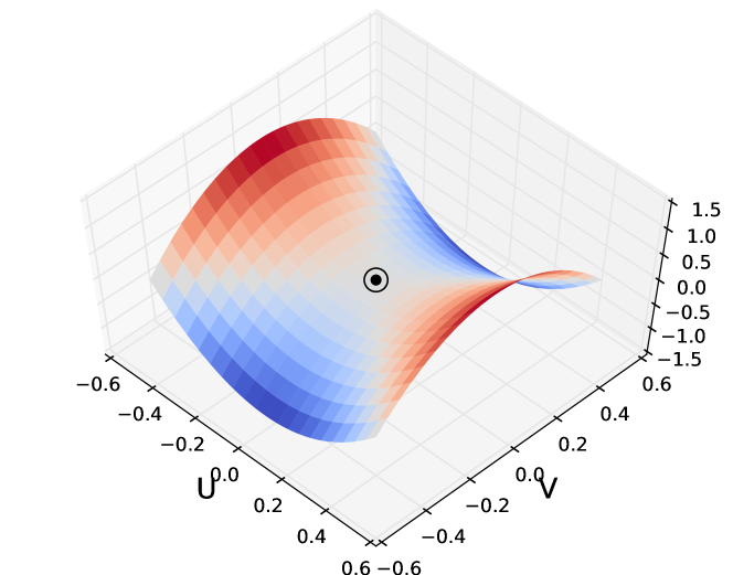
(a) Saddle ($u^{2}-v^{2}$)

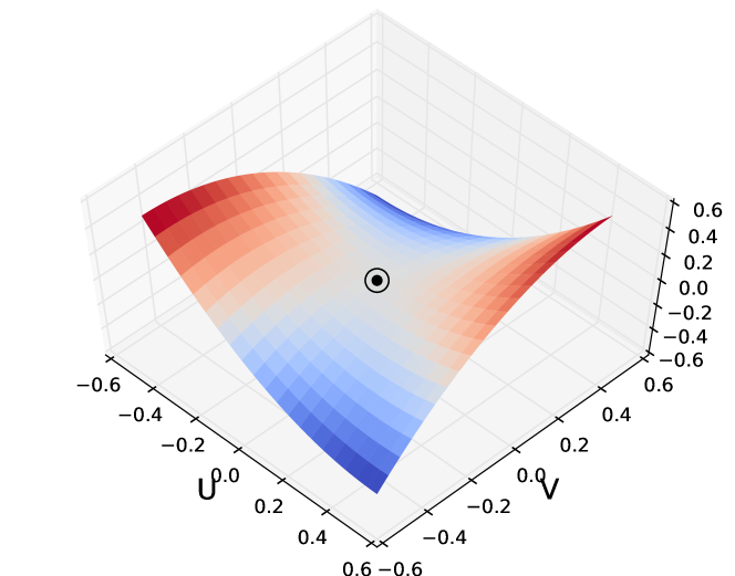
(b) Rotated saddle ($u^{2}-v^{2}+2uv$)

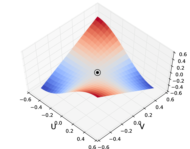
(c) Seesaw ($-v\sin(\pi u)$)

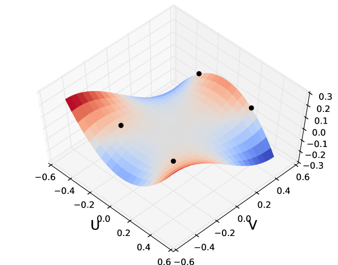
(d) Monkey saddle ($v^{3}-3vu^{2}$)

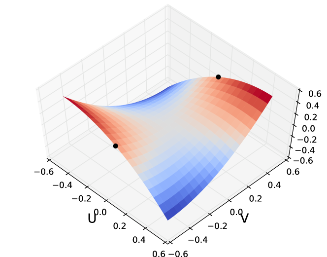
(e) Anti-saddle ($-u^{2}+v^{2}+2uv$)

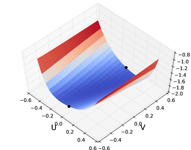
(f) Weapons (Danskin, 1967)
($e^{-10(u+.5)e^{-(v+.5)}}+e^{-10(.5-u)e^{v-.5}}$)

Figure 1: Saddle points (empty black circles) and minimax points (filled black circles). Surfaces (a),(b),(c) have both a saddle and minimax point at $(0,0)$, whereas surfaces (d),(e),(f) do not have global saddle points but only minimax points. All surfaces have a critical point at $(0,0)$.

Despite the fact that saddle points and minimax points are conceptually different, many machine learning applications in the literature do not distinguish the two. This is a mistake, because a local saddle point is only an equilibrium point and is not the robust or worst case solution that problem may be seeking. Furthermore, most papers have used the alternating gradient descent method

$$u\leftarrow u-\rho\nabla_{u}f(u,v),\;\;\mathrm{and}\;\;v\leftarrow v+\eta\nabla_{v}f(u,v).$$ (1)

Alternating descent fails to find minimax points even for 2-dimensional examples (d)-(f) in Fig. 1 as we show empirically in the Sec. 6.1. To explain the reason for failure, let’s define the inner maximum value $\phi(u):=\max_{v\in\mathcal{V}}f(u,v)$ and the corresponding maximum points $R(u):=\arg\max_{v\in\mathcal{V}}f(u,v)$. The main reason for failure is that the solution $R(u)$ may not be unique and can be discontinuous w.r.t. $u$. For example, in Fig. 1 (e), we have $R(u)=\{-0.5\}$ for $u<0$ and $R(u)=\{+0.5\}$ for $u>0$. This discontinuity at $u=0$ makes it impossible for a gradient descent-type method to keep track of the true inner maximization solution as $v$ has to jump between $\pm 0.5$.

In this paper, we propose a $K$-beam approach that tracks $K$ candidate solutions (or “beams”) of the inner maximization problem to handle the discontinuity. The proposed $\epsilon$-subgradient algorithm (Algs. 1 and  2) generalizes the alternating gradient-descent method ($K$=1) and also exact subgradient methods. In the analysis, we prove that it can find minimax points if the inner problem $\max_{v\in\mathcal{V}}f(u,v)$ can be approximated well by $\max_{v\in A}f(u,v)$ over a finite set $A$ at each $u$, summarized by Theorem 7 which is the main result of analysis. For the purpose of analysis we assume that $f$ is convex in $u$ similar to the majority of the analyses on gradient-type algorithms. However, we allow $f$ to be non-concave in $v$ and have multiple local maxima, which makes our setting much more general than that of classic saddle point problems with convex-concave $f$ or previous work which assumed only bilinear couplings between $u$ and $v$ (Chambolle & Pock, 2011; He & Yuan, 2012).

Practically, the algorithm can find solutions that gradient descent cannot find with only a sublinear increase of time complexity in $K$. To demonstrate the advantages of the algorithm, we test the algorithm on the toy surfaces (Fig. 1) for which we know the true minimax solutions. For real-world demonstrations, we also test the algorithm on GAN problems (Goodfellow et al., 2014), and unsupervised domain-adaptation problems (Ganin & Lempitsky, 2015). Examples were chosen so that the performance can be measured objectively – by the Jensen-Shannon divergence for GAN and by cross-domain classification error for domain adaptation. Evaluations show that the proposed $K$-beam subgradient-descent approach can significantly improve stability and convergence speed of minimax optimization.

The remainder of the paper is organized as follows. We discuss related work in Sec. 2 and backgrounds in Sec. 3. We propose the main algorithm in Sec. 4, and present the analysis in Sec. 5. The results of experiments are summarized in Sec. 6, and the paper is concluded in Sec. 7. Due to space limits, all proofs in Sec. 5 and additional figures are reported in Appendix. The codes for the project can be found at https://github.com/jihunhamm/k-beam-minimax.

2 Related work

Following the seminal work of Arrow et al. (1958) (Chap. 10 of Uzawa (1958) in particular), many researchers have studied the questions of the convergence of (sub)gradient descent for saddle point problems under different stability conditions (Dem’yanov & Pevnyi, 1972; Golshtein, 1972; Maistroskii, 1977; Zabotin, 1988; Nedić & Ozdaglar, 2009). Optimization methods for minimax problems have also been studied somewhat independently. The algorithm proposed by Salmon (1968), referred to as the Salmon-Daraban method by Dem’yanov & Pevnyi (1972), finds continuous minimax points by solving successively larger discrete minimax problems. The algorithm can find minimax points for a differentiable $f$ on compact $\mathcal{U}$ and $\mathcal{V}$. However, the Salmon-Daraban method is impractical, as its requires exact minimization and maximization steps at each iteration, and also because the memory footprint increases linearly with iteration. Another method of continuous minimax optimization was proposed by Dem’yanov & Malozemov (1971, 1974). The grid method, similar to the Salmon-Daraban method, iteratively solves a discrete minimax problem to a finite precision using the $\epsilon$-steepest descent method.

Recently, a large number of papers tried to improve GAN models in particular by modifying the objective (e.g.,Uehara et al. (2016); Nowozin et al. (2016); Arjovsky et al. (2017)), but relatively little attention was paid to the improvement of the optimization itself. Exceptions are the multiadversarial GAN (Durugkar et al., 2016), and the Bayesian GAN (Saatci & Wilson, 2017), both of which used multiple discriminators and have shown improved performance, although no analysis was provided. Also, gradient-norm regularization has been studied recently to stabilize gradient descent (Mescheder et al., 2017; Nagarajan & Kolter, 2017; Roth et al., 2017), which is orthogonal to and can be used simultaneously with the proposed method. Note that there can be multiple causes of instability in minimax optimization, and what we address here is more general and not GAN-specific.

3 Backgrounds

Throughout the paper, we assume that $f(u,v):\mathcal{U}\times\mathcal{V}\to\mathbb{R}$ is a continuously differentiable function in $u$ and $v$ separately. A general form of the minimax problem is $\inf_{u\in\mathcal{U}}\sup_{v\in\mathcal{V}}f(u,v)$. We assume that $\mathcal{U}$ and $\mathcal{V}$ are compact and convex subsets of Euclidean spaces such as a ball with a large but finite radius. Since $f$ is continuous, min and max values are bounded and attainable. In addition, the solutions to min or max problems are assumed to be in the interior of $\mathcal{U}$ ad $\mathcal{V}$, enforced by adding appropriate regularization (e.g, $\|u\|^{2}$ and $-\|v\|^{2}$) to the optimization problems if necessary.

As already introduced in Sec. 1, the inner maximum value and points are the key objects in the analysis of minimax problems.

Definition.

The maximum value $\phi(u)$ is $\max_{v\in\mathcal{V}}f(u,v)$.

Definition.

The corresponding maximum points $R(u)$ is $\arg\max_{v\in\mathcal{V}}f(u,v)$, i.e., $R(u)=\{v\in\mathcal{V}\;|\;f(u,v)=\max_{v\in\mathcal{V}}f(u,v)\}$.

Note that $\phi(u)$ and $R(u)$ are functions of $u$. With abuse of notation, the $R(\mathcal{U})$ is the union of maximum points for all $u\in\mathcal{U}$, i.e., $R(\mathcal{U}):=\bigcup_{u\in\mathcal{U}}R(u)$

As a generalization, the $\epsilon$-maximum points $R^{\epsilon}(u)$ are the points whose values are $\epsilon$-close to the maximum:
$R^{\epsilon}(u):=\{v\in\mathcal{V}\;|\;\max_{v\in\mathcal{V}}f(u,v)-f(u,v)\leq\epsilon\}$.

Definition.

$S(u)$ is the set of local maximum points

$$S(u) := \{v_{0}\in\mathcal{V}\;|\;\exists r>0\;\;s.t.\;\;\forall v\in\mathcal{V},$$

$$\;\;\;\;\;\;\|v_{0}-v\|\leq r\Rightarrow f(u,v_{0})\geq f(u,v)\}.$$

Note that $\nabla_{v}f(u,v)=0$ for $v\in S(u)$ due to differentiability assumption, and that $R(u)\subseteq S(u)$.

Definition.

$\min_{u\in\mathcal{U}}\max_{v\in A}f(u,v)$ is a discrete minimax problem if $A$ is a finite set $A:=\{v^{1},...,v^{K}\}\subseteq\mathcal{V}$.

We accordingly define $\phi_{A}(u)$, $R_{A}(u)$ and $R^{\epsilon}_{A}(u)$ by $\phi_{A}(u):=\max_{v\in A}f(u,v)$, and $R^{\epsilon}_{A}(u):=\{v\in A\;|\;\max_{v\in A}f(u,v)-f(u,v)\leq\epsilon\}$.

We also summarize a few results we will use, which can be found in convex analysis textbooks such as Hiriart-Urruty & Lemaréchal (2001).

Definition.

An $\epsilon$-subgradient of a convex function $\phi(u)$ at $u_{0}$ is $g\in\mathbb{R}^{d}$ that satisfies for all $u$

$$\phi(u)-\phi(u_{0})\geq\langle g,\;u-u_{0}\rangle-\epsilon.$$

The $\epsilon$-subdifferential $\partial_{\epsilon}\phi(u_{0})$ is the set of all $\epsilon$-subgradients at $u_{0}$.

Consider the convex hull $\mathrm{co}\{\cdot\}$ of the set of gradients.

Lemma 1 (Corollary 4.3.2, Theorem 4.4.2, Hiriart-Urruty & Lemaréchal (2001)).

Suppose $f(u,v)$ is convex in $u$ for each $v\in A$. Then $\partial\phi_{A}(u)=\mathrm{co}\{\cup_{v\in A}\nabla_{u}f(u,v)\}$. Similarly, suppose $f(u,v)$ is convex in $u$ for each $v\in\mathcal{V}$. Then $\partial\phi(u)=\mathrm{co}\{\cup_{v\in\mathcal{V}}\nabla_{u}f(u,v)\}$.

Definition.

A point $u$ is called an $\epsilon$-stationary point of $\phi_{A}(u)$ if $\max_{v\in R^{\epsilon}_{A}}\langle\nabla_{u}f(u,v),\;g\rangle\geq 0$ for all $g\in\mathbb{R}^{d}$.

Lemma 2 (Chap 3.6, Dem’yanov & Malozemov (1974)).

A point $u$ is an $\epsilon$-stationary point of $\phi(u)$ if and only if $0\in\mathrm{co}\{\cup_{v\in R^{\epsilon}(u)}\nabla_{u}f(u,v)\}$.

4 Algorithm

The alternating gradient descent method predominantly used in the literature fails when the inner maximization $\max_{v\in\mathcal{V}}f(u,v)$ has more than one solution, i.e., $R(u)$ is not a singleton. To address the problem, we propose the $K$-beam method to simultaneously track the maximum points $R(u)$ by keeping the candidate set $A=(v^{1},...,v^{K})$ for some large $K$. (The choice for $K$ will be discussed in Analysis and Experiments.) This approach can be exact, if the maximum points over the whole domain $R(\mathcal{U})$ is finite, as in examples (a),(e) and (f) of Fig. 1 (see Appendix.) In other words, the problem becomes a discrete minimax problem. More realistically, the maximum points $R(\mathcal{U})$ is infinite but $R(u)$ can still be finite for each $u$, as in all the examples of Fig. 1 except (c). At $i$-th iteration, the $K$-beam method updates the current candidates $A_{i}=(v^{1}_{i},...,v^{K}_{i})$ such that the discrete maximum $\phi_{A_{i}}(u)$ is a good approximation to the true $\phi(u)$. In addition, we present an $\epsilon$-subgradient algorithm that generalizes exact subgradient algorithms.

4.1 Details of the algorithm

Algorithm 1 $K$-beam $\epsilon$-subgradient descent

Input: $f,K,N,(\rho_{i}),(\eta_{i}),(\epsilon_{i})$
Output: $u_{N},A_{N}$
Initialize $u_{0},A_{0}=(v^{1}_{0},...,v^{K}_{0})$
Begin

  for $i=1,\;...\;,N$ do

     Min step:

     Update $u_{i}=u_{i-1}+\rho_{i}\;g(u_{i},A_{i},\epsilon_{i})$ where $g$ is a descent direction from Alg. 2.

     Max step:

     for $k=1,\;...\;,K$ in parallel do

        Update $v_{i}^{k}\leftarrow v_{i-1}^{k}+\eta_{i}\;\nabla_{v}f(u_{i},v_{i-1}^{k})$.

     end for

     Set $A_{i}=(v^{1}_{i},\;...\;,v^{K}_{i})$.

  end for

Alg. 1 is the main algorithm for solving minimax problems. At each iteration, the algorithm alternates between the min step and the max step. In the min step, it approximately minimizes $\phi(u)$ by following a subgradient direction $z\in\partial_{\epsilon}\phi_{A_{i}}(u)$. In the max step, it updates $A_{i}=\{v^{1}_{i},...,v^{K}_{i}\}$ to track the local maximum points of $f(u,\cdot)$ so that the approximate subdifferential $\partial_{\epsilon}\phi_{A_{i}}(u)$ remains close to the true subdifferential $\partial\phi(u)$.

The hyperparameters of the algorithm are the beam size ($K=|A|$), the total number of iterations ($N$), and the step size schedules for min step $(\rho_{i})$ and for max step $(\eta_{i})$ and the approximation schedule $(\epsilon_{i})$.

Algorithm 2 Descent direction

Input: $f,u,A=(v^{1},...,v^{K}),\epsilon$
Output: $g$
Begin

  Find $k_{\max}=\arg\max_{1\leq k\leq K}f(u,v^{k})$.

  Find $\{v^{k_{1}},...,v^{k_{n}}\}=R^{\epsilon}_{A}(u)=\{v\in A\;|\;f(u,v^{k_{\max}})-f(u,v^{k})\leq\epsilon\}$.

  Compute $z_{j}=\nabla_{u}f(u,v^{k_{j}})$ for $j=1,..,n$.

  Optional stopping criterion:

  if $0\in\mathrm{co}\{z_{1}\cup...\cup z_{n}\}$ then

     Found a stationary point. Quit optimization.

  end if

  Decent direction:

  if $n=1$ then

     Return $g=-z_{1}$.

  else

     Randomly choose $z\in\mathrm{co}\{z_{1}\cup...\cup z_{n}\}$ and return $g=-z$.

  end if

Alg. 2 is the subroutine for finding a descent direction. If $\epsilon$=0, this subroutine identifies the best candidate $v^{k_{\mathrm{max}}}$ among the current set $A_{i}$ and returns its gradient $\nabla_{u}f(u,v^{k_{\mathrm{max}}})$. If $\epsilon>0$, it finds $\epsilon$-approximate candidates and returns any direction in the convex hull of their gradients. We make a few remarks below.

• Alternating gradient descent (1) is a special case of the $K$-beam algorithm for $K=1$ and $\epsilon_{1}=\epsilon_{2}=...=0$.

• As will be shown in the experiments, the algorithm usually performs better with increasing $K$. However, increase in computation can be made negligible, since the $K$ updates in the max step can be performed in parallel.

• One can use different schemes for the step sizes $(\rho_{i}),(\eta_{i})$ and $(\epsilon_{i})$. For the purpose of analysis, we use non-summable but square-summable step size, e.g., $1/i$. Any decreasing sequence $(\epsilon_{i})\to 0$ can be used.

• The algorithm uses subgradients since the maximum value $\phi(u)$ is non-differentiable even if $f$ is, when there are more than one maximum point $(|R(u)|>1)$ (Danskin, 1967). In practice, when $\epsilon$ is close to 0, the approximate maximum set $R^{\epsilon}_{A}(u)$ in Alg. 2 is often a singleton in which case the descent direction from Alg. 2 is simply the gradient $-\nabla_{u}f(u,v)$.

• The convergence of the algorithm (Sec. 5) is not affected by the random choice $z\in\mathrm{co}\{z_{1}\cup...\cup z_{n}\}$ in Alg. 2. In practice, the random choice can help to avoid local minima if $f$ is not convex.

• Checking the stopping criterion $0\in\mathrm{co}\{\cup_{j}z_{j}\}$ can be non-trivial (see Sec. 5.4), and may be skipped in practice.

5 Analysis

We analyze the conditions under which Alg. 1 and Alg. 2 find a minimax point. We want the finite set $A_{i}$ at $i$-th iteration to approximate the true maximum points $R(u_{i})$ well, which we measure by the following two distances. Firstly, we want the following one-sided Hausdorff distance

$$d_{H}(R(u_{i}),A_{i}):=\max_{v\in R(u_{i})}\min_{v^{\prime}\in A_{i}}\|v-v^{\prime}\|$$ (2)

to be small, i.e., each global maximum $v\in R(u_{i})$ is close to at least one candidate in $A_{i}$. Secondly, we also want the following one-sided Hausdorff distance

$$d_{H}(A_{i},S(u_{i})):=\max_{v^{\prime}\in A_{i}}\min_{v\in S(u_{i})}\|v-v^{\prime}\|$$ (3)

to be small, where $S(u_{i})$ is the local maxima, i.e., each candidate is close to at least one local maximum $v\in S(u_{i})$. This requires that $K$ is at least as large as $\max_{u}|S(u)|$.

We discuss the consequences of these requirements more precisely in the rest of the section. For the purpose of analysis, we will make the following additional assumptions.
Assumptions. $\phi(u)$ is convex and achieves the minimum $\phi^{\ast}=\phi(u^{\ast})$. Also, $f(u,v)$ is $l$-Lipschitz in $v$ for all $u$, and $\nabla_{u}f(u,v)$ is $r$-Lipschitz in $v$ for all $u$.

Remark on the assumption. Note that we only assume the convexity of $f$ over $u$ and not the concavity over $v$, which makes this setting more general than that of classic analyses which assume the concavity over $v$, or that of restricted models with a bilinear coupling $f(u,v)=f_{\mathrm{convex}}(u)+g_{\mathrm{concave}}(v)+u^{T}Av$. While we allow $f$ to be non-concave in $v$ and have multiple local maxima, we also require $f$ and $\nabla_{u}f$ to be Lipschitz in $v$ for the purpose of analysis.

5.1 Finite $R(u)$, exact max step

If $R(u)$ is finite for each $u$, and if the maximization in the max step can be done exactly as assumed in the Salmon-Daraban method (Salmon, 1968), then the problem is no more difficult than a discrete minimax problem.

Lemma 3.

Suppose $R(u)$ is finite at $u$. If $d_{H}(R(u),A)=0$, then $R(u)=R_{A}(u)$ and therefore $\partial\phi(u)=\partial\phi_{A}(u)$.

Since the subdifferential is exact, Alg. 1 finds a minimax solution as does the subgradient-descent method with the true $\phi(u)$. We omit the proof and present a more general theorem shortly.

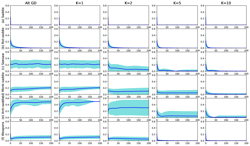
Figure 2: Convergence of Alt-GD and $K$-beam ($K=1,2,5,10$) for the six surfaces (Fig. 1) after 200 iterations, measured by the distance to the closest optimal point. The dark blue line is the average error and the light blue area is the avg$\pm$std. For easy surfaces (a) and (b), all methods converge quickly. For surfaces (c)-(f), Alt-GD fails to converge to the solution whereas $K$-beam does with $K>1$.

5.2 Finite $R(u)$, inexact max step

Exact maximization in each max step is unrealistic, unless $\max_{v}f(u,v)$ can be solved in closed form. Therefore we consider what happens to the convergence of the algorithm with an approximate max step. If $d_{H}(R(u),A)\leq\delta$ and $d_{H}(A,S(u))\leq\delta$ for some $\delta\geq 0$, how close are $\phi(\cdot)$ and $\phi_{A}(\cdot)$ in the vicinity of $u$? The following lemmas answer this question. (See Appendix for a visual aid.) From the smoothness assumptions on $f$, we have

Lemma 4.

If $d_{H}(R(u),A)\leq\delta$, then for each $v\in R(u)$ there is one or more $v^{\prime}\in A$ such that $\phi(u)-f(u,v^{\prime})\leq l\delta$ and $\|\nabla_{u}f(u,v)-\nabla_{u}f(u,v^{\prime})\|\leq r\delta$.

The following lemma shows that if $A$ approximates $R(u)$ well, then $v^{\prime}$ chosen by Alg. 2 is not far from a true maximum $v\in R(u)$.

Lemma 5.

Assume $R(u)$ and $S(u)$ are both finite at $u$. Let $\zeta=\phi(u)-\max_{v\in S(u)\setminus R(u)}f(u,v)$ be the smallest gap between the global and the non-global maximum values at $u$. If all local maxima are global maxima, then set $\zeta=\infty$. If $d_{H}(R(u),A)\leq\delta$ and $d_{H}(A,S(u))\leq\delta$ where $\delta<0.5(\zeta-\epsilon)/l$, then for each $v^{\prime}\in R^{\epsilon}_{A}(u)$, there is $v\in R(u)$ such that $\|v-v^{\prime}\|\leq\delta$.

Furthermore, the subgradients at the approximate maximum points are close to the subgradients at the true maximum points.

Lemma 6.

Suppose $\delta$ is chosen as in Lemma 5 and $\mathcal{U}$ is bounded: $\max_{u\in\mathcal{U}}\|u\|=B$. Then any $z^{\prime}\in\mathrm{co}$ $\{\cup_{v\in{R^{\epsilon}_{A}}}\nabla_{u}f(u_{0},v)\}$ is an $(2r\delta B)$-subgradient of $\phi(u_{0})$.

Now we state our main theorem that if the max step is accurate enough for a large $i$ in terms of $\zeta_{i}$ (a property of $f$) and $\epsilon_{i},\xi_{i}$ (chosen by a user), then the algorithm finds the minimum value using a step size $\rho_{i}\sim 1/i$.

Theorem 7.

Suppose the conditions of Lemmas 4, 5 and  6 hold, and also suppose the max step in Alg. 1 is accurate for sufficiently large $i\geq i_{0}$ for some $i_{0}\geq 1$ so that $\max[d_{H}(R(u_{i}),A_{i}),d_{H}(A_{i},S(u_{i}))]\leq\delta_{i}$ holds where $\delta_{i}\leq\min\left[0.5(\zeta_{i}-\epsilon_{i})/l,\;0.5\xi_{i}/(rB)\right]$ for some non-negative sequence $(\xi_{1},\xi_{2},...).$ If the step size satisfies $\rho_{i}\geq 0,\forall i$, $\sum_{i=1}^{\infty}\rho_{i}=\infty$, $\sum_{i=1}^{\infty}\rho_{i}^{2}<\infty$, and $\sum_{i=1}^{\infty}\rho_{i}\xi_{i}<\infty$, then $\min[\phi(u_{1}),...,\phi(u_{i})]$ converges to the minimum value $\phi^{\ast}$.

For $\rho_{i}$ and $\xi_{i}$ we can also use $1/i$. The $\epsilon_{i}$ can be any non-negative value. A large $\epsilon_{i}$ can make each min step better since the descent direction in Alg. 2 uses more $z_{i}$’s and therefore is more robust. The price to pay is that it may take more iterations for the max step to meet the condition $\delta_{i}\leq\min\left[0.5(\zeta_{i}-\epsilon_{i})/l,\;0.5\xi_{i}/(rB)\right]$.

5.3 Infinite $R(u)$

Infinite $R(u)$ is the most challenging case. We only mention the accuracy of the approximating $R(u)$ with a finite and fixed $A$ as in the grid methods of Dem’yanov & Malozemov (1971, 1974).

Lemma 8.

For any $\epsilon>0$, one can choose a fixed $A=(v^{1},...,v^{K})$ such that $\phi(u)-\phi_{A}(u)\leq\epsilon$ holds for all $u$. Furthermore, if $\hat{u}=\arg\min_{u}\phi_{A}(u)$ is the minimizer of the approximation, then $\phi(\hat{u})-\phi(u^{\ast})\leq\epsilon$.

If $A$ is dense enough, the solution $\hat{u}$ can be made arbitrarily accurate, but the corresponding $K=|A|$ can be too large and has to be limited in practice.

5.4 Optional stopping criteria

The function $\phi(u)$ is non-smooth and its gradient need not vanish at the minimum, causing oscillations. A stopping criterion can help to terminate early. We can stop at an $\epsilon$-stationary point of $\phi(u)$ by checking if $0\in\partial_{\epsilon}\phi(u)$ from Lemma 2. Algorithmically, this check is done by solving a LP or a QP problem (Dem’janov, 1968). The stopping criterion presented in Alg. 2 is a necessary condition for the approximate stationarity of $\phi(u)$:

Lemma 9.

Let $\epsilon=\epsilon^{\prime}+l\delta$ $(\epsilon,\epsilon^{\prime}\geq 0)$ where $l$ is the Lipschitz coefficient of $f(u,v)$ in $v$. If $u_{0}$ is an $\epsilon$-stationary point of $\phi(u)$, then $u_{0}$ is an $\epsilon^{\prime}$-stationary point of $\phi_{A}(u)$.

The size $n$ of the QP problem is $|R^{\epsilon}_{A}(u)|$ which is small for $\epsilon\ll 1$, but it can be costly to solve at every iteration. It is therefore more practical to stop after a maximum number of iterations or by checking the stopping criterion only every so often.

6 Experiments

6.1 Simple surfaces

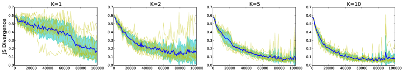
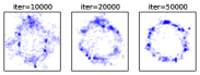
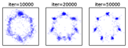
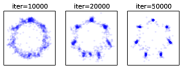
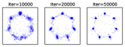
Figure 3: Top row: Jensen-Shannon divergence vs iteration for GAN training with MoG. The dark blue line is the average divergence and the light blue area is the avg$\pm$std. The light yellow lines are traces of 10 independent trials. Training is more stable and faster with a larger $K$. Bottom row: Corresponding samples generated after 10000, 20000, and 50000 iterations.

We test the proposed algorithm to find minimax points of the simple surfaces in Fig. 1. We compare Alternating Gradient Descent (Alt-GD), and the proposed $K$-beam algorithm with $K=1,2,5,10$. Note that for $K=1$, the minimax algorithm is basically the same as Alt-GD. Since the domain is constrained to $[-0.5,0.5]^{2}$, we use the projected gradient at each step with the common learning rate of $\rho_{i}=\eta_{i}=0.1/i$. In our preliminary tests, the value of $\epsilon_{i}$ in Alg. 1 did not critically affect the results, and we report the case $\epsilon_{i}=0$ for all subsequent tests. The experiments are repeated for 100 trials with random initial conditions.

Fig. 2 shows the convergence of Alt-GD and $K$-beam ($K=1,2,5,10$) after 200 iterations, measured by the distance of the current solution to the closest optimal point $d(u_{i},U^{\ast}):=\min_{u\in U^{\ast}}\|u_{i}-u\|$, where $U^{\ast}$ is the set of minimax solutions. We plot the average and the confidence level of the 100 trials. All methods converge well for surfaces (a) and (b). The surface (c) is more difficult. Although $(0,0)$ is a saddle point, (i.e., $0=f(0,v)\leq f(0,0)\leq f(u,0)=0,\;\forall u,v$), the point $(0,0)$ is unstable as it has no open neighborhood in which $f$ is a local minimum in $u$ and a local maximum in $v$. For non-saddle point problems (d)-(e), one can see that Alt-GD simply cannot find the true solution, whereas $K$-beam can find the solution if $K$ is large enough. For anti-saddle (e), $K=2$ is the smallest number to find the solution since the local maximum point $|S(u)|$ is at most 2. However, concavity-convexity of $f$ (instead of convexity-concavity) makes optimization difficult and therefore $K>2$ helps to recover from bad random initial points and find the solution.

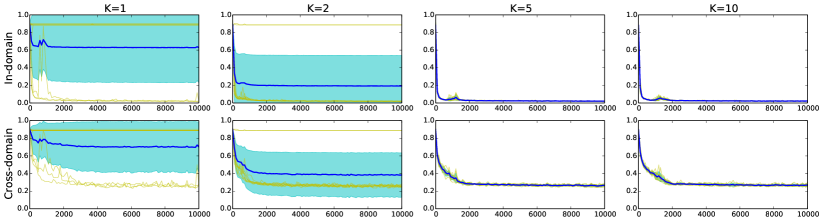
Figure 4: Test error vs iteration for MNIST and MNISTM. The top/bottom row corresponds to in-domain/cross-domain results, respectively. The dark blue line is the average error and the light blue area is the avg$\pm$std. The light yellow lines are traces of 10 independent trials. For $K$=1 or 2, some trials fail to converge at all. With $K$=5 or 10, all trials converge to $0.02$ (in-domain) and $0.27$ (cross-domain).

6.2 GAN training with MoG

We train GANs with the proposed algorithm to learn a generative model of two-dimensional mixtures of Gaussians (MoGs). Let $x$ be a sample from the MoG with the density $p(x)=\frac{1}{7}\sum_{i=0}^{6}\mathcal{N}\left((\sin(\pi i/4),\cos(\pi i/4)),\;(0.01)^{2}I_{2}\right)$,

and $z$ be a sample from the 256-dimensional Gaussian distribution $\mathcal{N}(0,I_{256})$. The optimization problem is

$$\min_{u}\max_{v}E\left[\log D(x;v)+\log(1-D(G(z;u);v))\right],$$

where $G(z;u)$ and $D(x;v)$ are generator and discriminator networks respectively. Both $G$ and $D$ are two-layer tanh networks with 128 hidden units per layer, trained with Adam optimizer with batch size 128 and the learning rate of $10^{-4}$ for the discriminator and $10^{-3}$ for the generator.

For evaluation, we measure the Jensen-Shannon divergence

$$\mathrm{JSD}=\frac{1}{2}\mathrm{KL}\left(P,\frac{P+Q}{2}\right)+\frac{1}{2}\mathrm{KL}\left(Q,\frac{P+Q}{2}\right)$$

between the true MoG $P$ and the samples $Q$ from the generator. We measure the divergence by discretizing the 2D region into $20\times 20$ bins and compare the histograms of 64,000 random samples from the generator and 640,000 samples from the MoG. The top row, Fig. 3, shows the JSD curves of $K$-beam with $K$=1,2,5,10. Alt-GD performs nearly the same as $K$=1 and is omitted. The results are from 10 trials with random initialization. Note first that GAN training is sensitive in that each trial curve is jagged and often falls into the “mode collapsing” where there is a jump in the curve. With $K$ increasing, the curve converges faster on average and is more stable as evidenced by the shrinking variance. The bottom row, Fig. 3, shows the corresponding samples from the generators after 10,000, 20,000, and 50,000 iterations from all 10 trials. The generated samples are also qualitatively better with $K$ increasing.

Additionally, we measure the runtime of the algorithms by wall clock on the same system using a single NVIDIA GTX980 4GB GPU with a single Intel Core i7-2600 CPU. Even on a single GPU, the runtime per iteration increases only sublinear in K: relative to the time required for $K$=1, we get $\times$1.07 ($K$=2), $\times$1.63 ($K$=5), and $\times$2.26 ($K$=10). Since the advantages are clear and the incurred time is negligible, there is a strong motivation to use the proposed method instead of Alt-GD.

6.3 Unsupervised domain adaptation

We perform experiments on unsupervised domain adaptation (Ganin & Lempitsky, 2015) which is another example of minimax problems. In domain adaption, it is assumed that two data sets belonging to different domains share the same structure. For examples, MNIST and MNIST-M are both images of handwritten digits 0–9, but MNIST-M is in color and has random background patches. Not surprisingly, the classifier trained on MNIST does not perform well with digits from MNIST-M out of the box. Unsupervised domain adaption tries to learn a common transformation $G$ of the domains into another representation/features such that the distributions of the two domains are as similar as possible while preserving the digit class information. The discriminator $D_{1}$ tries to predict the domain accurately, and the target classifier $D_{2}$ tries to predict the label correctly. The optimization problem can be rewritten as $\min_{u=\{u^{\prime},w\}}\max_{v}f(u,v)$ with

$$f(u,v)=-E[D_{1}(G(x;u^{\prime});v)]+\lambda\;E[D_{2}(G(x;u^{\prime});w)],$$

which is the weighted difference of the expected risks of the domain classifier $D_{1}$ and the digit classifier $D_{2}$. This form of minimax problem has also been proposed earlier by Hamm (2015, 2017) to remove sensitive information from data. In this experiment, we show domain adaptation results. The transformer $G$ is a two-layer ReLU convolutional network that maps the input features (=images) to an internal representation of dim=2352. The discriminator $D_{1}$ is a single-layer ReLU dense network of 100 hidden units, and the digit classifier $D_{2}$ is a two-layer ReLU dense network of 100 hidden units. All networks are trained with the momentum optimizer with the batch size of 128 and the learning rate of $10^{-2}$. The experiments are repeated for 10 trials with random initialization. We use $\lambda=1$.

We performed the task of predicting the class of MNISTM digits, trained using labeled examples of MNIST and unlabeled examples of MNISTM. Fig. 4 shows the classification error of in-domain (top row) and cross-domain (bottom row) prediction tasks as a function of iterations. Again we omit the result of Alt-GD as it performs nearly the same as $K$=1. With $K$ small, the average error is high for both in-domain and cross-domain tests, due to failed optimization which can be observed in the traces of the trials. As $K$ increases, instability disappears and both in-domain and cross-domain errors converge to their lowest values.

Summary and discussions

• Experiments with 2D surfaces clearly show that the alternating gradient-descent method can fail completely when the minimax points are not local saddle points, while the $K$-beam method can find the true solutions.

• For GAN and domain adaptation problems involving nonlinear neural networks, the $K$-beam and Alt-GD can both find good solutions if they converge. The key difference is, the $K$-beam consistently converges to a good solution, whereas Alt-GD finds the solution only rarely (which are the bottom yellow curves for $K$=1 in Fig. 3 and Fig. 4.) Similar results can be observed in GAN-MNIST experiments in Appendix.

• The true $K$ value cannot be computed analytically for nontrivial functions. However, an overestimated $K$ does not hurt the performance theoretically – it is only redundant. One the other hand, an underestimated $K$ can be suboptimal but is still better than $K$=1. Therefore, in practice, one can choose as large a number as allowed by resource limits such as $K$=5 or 10.

• The $K$-beam method is different from running Alt-GD for $K$-times more iterations, since the instability of Alt-GD hinders convergence regardless of the total number of iterations. The $K$-beam method is also different from $K$-parallel independent runs of Alt-GD, which are basically the figures of $K$=1 in Fig. 3 and Fig. 4, but with $K$-times more trials. The variance will be reduced but the average curve will remain similar.

7 Conclusions

In this paper, we propose the $K$-beam subgradient descent algorithm to solve continuous minimax problems that appear frequently in machine learning. While simple in implementation, the proposed algorithm can significantly improve the convergence of optimization compared to the alternating gradient descent approach as demonstrated by synthetic and real-world examples. We analyze the conditions for convergence without assuming concavity or bilinearity, which we believe is the first result in the literature. There are open questions regarding possible relaxations of assumptions used which are left for future work.

Appendix

Appendix A Simple surfaces

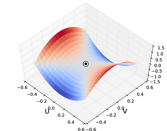
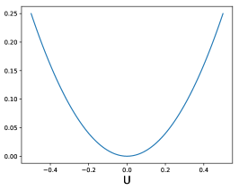
(a) Saddle ($u^{2}-v^{2}$)
critical pts $\{(0,0)\}$ saddle pts $\{(0,0)\}$ minimax pts $\{(0,0)\}$

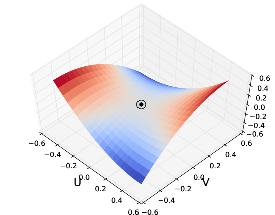
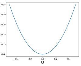
(b) Rotated saddle ($u^{2}-v^{2}+2uv$) critical pts $\{(0,0)\}$ saddle pts $\{(0,0)\}$ minimax pts $\{(0,0)\}$

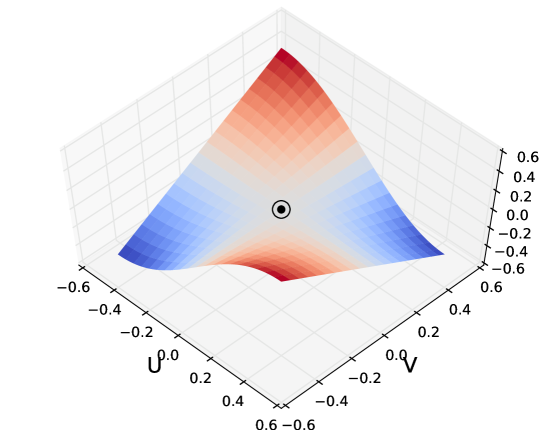
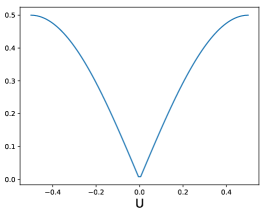
(c) Seesaw ($-v\sin(\pi u)$) critical pts $\{(0,0)\}$ saddle pts $\{(0,0)\}$ minimax pts $\{(0,v)|v\in[-0.5,0.5])\}$

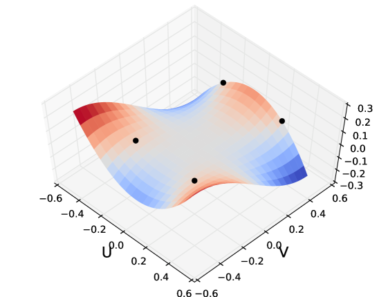
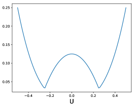
(d) Monkey saddle ($v^{3}-3vu^{2}$) critical pts $\{(0,0)\}$ saddle pts $\{\}$ minimax pts $\{(\pm 0.25,-0.25),(\pm 0.25,0.5)\}$

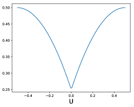
(e) Anti-saddle ($-u^{2}+v^{2}+2uv$) critical pts $\{(0,0)\}$ saddle pts $\{\}$ minimax pts $\{(0,\pm 0.5)\}$

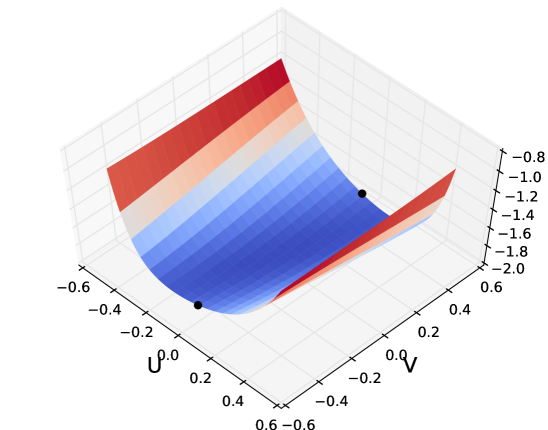
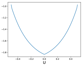
(f) Weapons ($e^{-10(u+.5)e^{-(v+.5)}}+e^{-10(.5-u)e^{v-.5}}$) critical pts $\{(0,0)\}$ saddle pts $\{\}$ minimax pts $\{(0,\pm 0.5)\}$

Figure 5: Examples of saddle point (top row) and non-saddle point (bottom row) problems. The smaller inset after each surface is the max value function $\phi(u)=\max_{v}f(u,v)$.

Fig.1 shows the six surfaces $f(u,v)$ and the maximum value function $\phi(u)=\max_{v\in\mathcal{V}}f(u,v)$. From $\phi(u)$ one can check the minima $\arg\min_{u}\phi(u)$ are:
(a) $u=0$, (b) $u=0$, (c) $u=0$, (d) $u=\pm 0.25$, (e) $u=0$, and (f) $u=0$.
The corresponding maxima $R(u)=\arg\max_{v\in\mathcal{V}}f(u,v)$ at the minimum are:
(a) $R(0)=\{0\}$, (b) $R(0)=\{0\}$, (c) $R(0)=[-0.5,0.5]$, (d) $R(\pm 0.25)=\{-0.25,0.5\}$, (e) $R(0)=\{-0.5,0.5\}$, and (f) $R(0)=\{-0.5,0.5\}$.

Furthermore, $R(\mathcal{U})$ for the whole domain is:
(a) $R(\mathcal{U})=\{0\}$, (b) $R(\mathcal{U})=[-0.5,0.5]$, (c) $R(\mathcal{U})=\{-0.5,0.5\}$ except for $R(0)=[-0.5,0.5]$, (d) $R(\mathcal{U})=[-0.5,-0.25]\cup\{0.5\}$, (e) $R(\mathcal{U})=\{-0.5,0.5\}$, and (f) $R(\mathcal{U})=\{-0.5,0.5\}$. These can be verified by solving the minimax problems in closed form.

Note that the origin $(0,0)$ is a critical point for all surfaces. It is also a global saddle point and minimax point for surfaces (a)-(c), but is neither a saddle nor a minimax point for surfaces (d)-(f).

Appendix B Proofs

Lemma 1 (Corollary 4.3.2, Theorem 4.4.2, (Hiriart-Urruty & Lemaréchal, 2001)).

Suppose $f(u,v)$ is convex in $u$ for each $v\in A$. Then $\partial\phi_{A}(u)=\mathrm{co}\{\cup_{v\in A}\nabla_{u}f(u,v)\}$. Similarly, suppose $f(u,v)$ is convex in $u$ for each $v\in\mathcal{V}$. Then $\partial\phi(u)=\mathrm{co}\{\cup_{v\in\mathcal{V}}\nabla_{u}f(u,v)\}$.

Lemma 2 (Chap 3.6, (Dem’yanov & Malozemov, 1974)).

A point $u$ is an $\epsilon$-stationary point of $\phi_{A}(u)$ if and only if $0\in\mathrm{co}\{\cup_{v\in R^{\epsilon}_{A}(u)}\nabla_{u}f(u,v)\}$.

Lemma 3.

Suppose $R(u)$ is finite at $u$. If $d_{H}(R(u),A)=0$, then $R(u)=R_{A}(u)$ and therefore $\partial\phi(u)=\partial\phi_{A}(u)$.

Proof.

Since $A\subseteq\mathcal{V}$ , $\max_{v\in\mathcal{V}}f(u,v)=\max_{v\in R(u)}$ $f(u,v)\geq\max_{v\in A}f(u,v)$. By $d_{H}(R(u),A)=0$, we have $R(u)\subseteq A$ and therefore for each $v\in R(u)$, $f(u,v)=\max_{v\in\mathcal{V}}f(u,v)=\max_{v\in A}f(u,v)$, so $v\in R_{A}(u)$. Conversely, if $v\in R_{A}(u)$ then $f(u,v)=\max_{v\in A}f(u,v)=\max_{v\in\mathcal{V}}f(u,v)$, so $v\in R(u)$. The remainder of the theorem follows from the definition of subdifferentials. ∎

Fig. 6 explains several symbols used in the following lemmas.

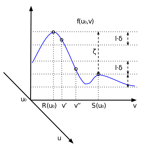
Figure 6: Consider a slice of $f(u,v)$ at $u=u_{0}$. $\zeta$: smallest gap between the $f$ values of global maxima $R(u)$ and non-global maxima $S(u)\setminus R(u)$. $v^{\prime}$ is no farther than $\delta$ to a point in $R(u_{0})$ and $v^{\prime\prime}$ is no farther than $\delta$ to a point in $S(u_{0})\setminus R(u_{0})$. By choosing $\epsilon<\zeta-2l\delta$, we have $v^{\prime}\in R^{\epsilon}_{A}(u_{0})$ and $v^{\prime\prime}\notin R^{\epsilon}_{A}(u_{0})$. See Lemma 5.

Lemma 4.

If $d_{H}(R(u),A)\leq\delta$, then for each $v\in R(u)$ there is one or more $v^{\prime}\in A$ such that $\phi(u)-f(u,v^{\prime})\leq l\delta$ and $\|\nabla_{u}f(u,v)-\nabla_{u}f(u,v^{\prime})\|\leq r\delta$.

The proof follows directly from the Lipschitz assumptions.

Lemma 5.

Assume $R(u)$ and $S(u)$ are both finite at $u$. Let $\zeta=\phi(u)-\max_{v\in S(u)\setminus R(u)}f(u,v)$ be the smallest gap between the global and the non-global maximum values at $u$. If all local maxima are global maxima, then set $\zeta=\infty$. If $d_{H}(R(u),A)\leq\delta$ and $d_{H}(A,S(u))\leq\delta$ where $\delta<0.5(\zeta-\epsilon)/l$, then for each $v^{\prime}\in R^{\epsilon}_{A}(u)$, there is $v\in R(u)$ such that $\|v-v^{\prime}\|\leq\delta$.

Proof.

Let any $v^{\prime}\in A$ be $\delta$-close to a global maximum, then $f(u,v^{\prime})\geq\phi(u)-l\delta$. Similarly, let any $v^{\prime\prime}\in A$ be $\delta$-close to a non-global maximum, then $f(u,v^{\prime\prime})\leq\phi(u)-(\zeta-l\delta)$. Consequently, $f(u,v^{\prime})\geq f(u,v^{\prime\prime})+\zeta-2l\delta>f(u,v^{\prime\prime})+\epsilon$, i.e., any $f(u,v^{\prime})$ and $f(u,v^{\prime\prime})$ are separated by at least $\epsilon$. Therefore, each $v^{\prime}$ satisfies $v^{\prime}\in R^{\epsilon}_{A}=\{v\in A\;|\;\phi_{A}(u)-f(u,v)\leq\epsilon\}$ but no $v^{\prime\prime}$ satisfies $v^{\prime\prime}\in R^{\epsilon}_{A}$. ∎

Lemma 6.

Suppose $\delta$ is chosen as in Lemma 5 and $\mathcal{U}$ is bounded ($\forall u\in\mathcal{U},\;\|u\|=B<\infty$.) Then any $z^{\prime}\in\mathrm{co}\{\cup_{v\in{R^{\epsilon}_{A}}}\nabla_{u}f(u_{0},v)\}$ is an $(2r\delta B)$-subgradient of $\phi(u_{0})$.

Proof.

From Lemmas 4 and  5, for each $(v^{k})^{\prime}\in R^{\epsilon}_{A}$, there is $v^{k}\in R(u_{0})$ such that $\|\nabla_{u}f(u_{0},v^{k})-\nabla_{u}f(u_{0},(v^{k})^{\prime})\|\leq r\delta.$ Let $z_{k}=\nabla_{u}f(u_{0},v^{k})$ and $z^{\prime}_{k}=\nabla_{u}f(u_{0},(v^{k})^{\prime})$. Then, for all $k=1,...,|R^{\epsilon}_{A}|$ and for all $u$,

$$\phi(u)-\phi(u_{0})-\langle z_{k}^{\prime},\;u-u_{0}\rangle$$

$$= \phi(u)-\phi(u_{0})-\langle z_{k}+z^{\prime}_{k}-z_{k},\;u-u_{0}\rangle$$

$$\geq -\langle z^{\prime}_{k}-z_{k},\;u-u_{0}\rangle$$

$$\geq -\|z^{\prime}_{k}-z_{k}\|\|u-u_{0}\|$$

$$\geq -r\delta\|u-u_{0}\|\geq-2r\delta B.$$

By taking any convex combination of $\sum_{k=1}^{n}a_{k}(\cdot)$ on both sides, we have

$$\phi(u)-\phi(u_{0})-\langle\sum_{k=1}^{n}a_{k}z^{\prime}_{k},\;u-u_{0}\rangle\geq-2r\delta B,$$

and therefore any $z^{\prime}\in\mathrm{co}\{\cup_{v\in{R^{\epsilon}_{A}}}\nabla_{u}f(u_{0},v)\}$ is a $(2r\delta B)$-subgradient of $\phi(u_{0})$ ∎

Theorem 7.

Suppose the conditions of Lemmas 4, 5 and  6 hold, and also suppose the max step in Alg.2 is accurate for sufficiently large $i\geq i_{0}$ for some $i_{0}\geq 1$ so that $\max[d_{H}(R(u_{i}),A_{i}),d_{H}(A_{i},S(u_{i}))]\leq\delta_{i}$ holds where $\delta_{i}\leq\min\left[0.5(\zeta_{i}-\epsilon_{i})/l,\;0.5\xi_{i}/(rB)\right]$ for some non-negative sequence $(\xi_{1},\xi_{2},...).$ If the step size satisfies $\rho_{i}\geq 0,\forall i$, $\sum_{i=1}^{\infty}\rho_{i}=\infty$, $\sum_{i=1}^{\infty}\rho_{i}^{2}<\infty$, and $\sum_{i=1}^{\infty}\rho_{i}\xi_{i}<\infty$, then $\min[\phi(u_{1}),...,\phi(u_{i})]$ converges to the minimum value $\phi^{\ast}$.

Note that a stronger result such as $\lim\inf_{i\to\infty}\phi(u_{i})=\phi^{\ast}$ is possible (see, e.g., (Correa & Lemaréchal, 1993)), but we give a simpler proof similar to (Boyd et al., 2003) which assumes $\|\nabla_{u}f(u,v)\|\leq L$ for some $L>0$.

Proof.

We combine previous lemmas with the standard proof of the $\epsilon$-subgradient descent method. Let $u_{i+1}=u_{i}-\rho_{i}g_{i}$. Then,

$$\|u_{i+1}-u^{\ast}\|^{2}$$

$$= \|u_{i}-u^{\ast}\|^{2}+\rho_{i}^{2}\|g_{i}\|^{2}+2\rho_{i}\langle g_{i},\;u^{\ast}-u_{i}\rangle$$

$$\leq \|u_{i}-u^{\ast}\|^{2}+\rho_{i}^{2}\|g_{i}\|^{2}+2\rho_{i}(\phi(u^{\ast})-\phi(u_{i})+\xi_{i})$$

from the definition of $\partial_{\xi}\phi(u)$. Taking $\sum_{i=1}^{N}(\cdot)$ on both sides gives us

$$\|u_{N+1}-u^{\ast}\|^{2} \leq \|u_{1}-u^{\ast}\|^{2}+\sum_{i=1}^{N}\rho_{i}^{2}\|g_{i}\|^{2}$$

$$+2\sum_{i=1}^{N}\rho_{i}(\phi(u^{\ast})-\phi(u_{i})+\xi_{i}),$$

or equivalently,

$$2\sum_{i=1}^{N}(\rho_{i}(\phi(u_{i})-\phi(u^{\ast})-\xi_{i})\leq\|u_{1}-u^{\ast}\|^{2}+\sum_{i=1}^{N}\rho_{i}^{2}\|g_{i}\|^{2}.$$

If we define $\underline{\phi}(u_{i}):=\min[\phi(u_{1}),...,\phi(u_{i})]$, then $\sum_{i=1}^{N}\rho_{i}(\phi(u_{i})-\phi^{\ast})\geq(\sum_{i=1}^{N}\rho_{i})(\underline{\phi}(u_{i})-\phi^{\ast})$. Combining the two inequalities, we have

$$0 \leq \underline{\phi}(u_{i})-\phi^{\ast}\leq\frac{\sum_{i=1}^{N}\rho_{i}(\phi(u_{i})-\phi^{\ast})}{\sum_{i=1}^{N}\rho_{i}}$$

$$\leq \frac{\|u_{1}-u^{\ast}\|^{2}+\sum_{i=1}^{N}\rho_{i}^{2}\|g_{i}\|^{2}+2\sum_{i=1}^{N}\rho_{i}\xi_{i}}{2\sum_{i=1}^{N}\rho_{i}}$$

$$\leq \frac{\|u_{1}-u^{\ast}\|^{2}+\sum_{i=1}^{N}\rho_{i}^{2}L^{2}+2\sum_{i=1}^{N}\rho_{i}\xi_{i}}{2\sum_{i=1}^{N}\rho_{i}}.$$

With $\sum_{i=1}^{\infty}\rho_{i}=\infty$, $\sum_{i=1}^{\infty}\rho_{i}^{2}<\infty$, and $\sum_{i=1}^{\infty}\rho_{i}\xi_{i}<\infty$, we get $\underline{\phi}(u_{i})\to\phi^{\ast}$. ∎

Lemma 8.

For any $\epsilon>0$, one can choose a fixed $A=(v^{1},...,v^{k})$ such that $\phi(u)-\phi_{A}(u)\leq\epsilon$ holds for all $u$. Furthermore, if $\hat{u}=\arg\min_{u}\phi_{A}(u)$ is the minimizer of the approximation, then $\phi(\hat{u})-\phi(u^{\ast})\leq\epsilon$.

Proof.

Since $\mathcal{V}$ is compact and $f$ is continuous, we can find a finite grid $A$ such as a uniform $\epsilon/l$-grid for $l$-Lipschitz $f$ so that $\phi(u)-\phi_{A}(u)\leq\epsilon$ for all $u$. Furthermore, we have

$$\phi(\hat{u})-\phi(u^{\ast}) = \phi(\hat{u})-\phi_{A}(\hat{u})+\phi_{A}(\hat{u})-\phi(u^{\ast})$$

$$\leq \phi(\hat{u})-\phi_{A}(\hat{u})+\phi_{A}(u^{\ast})-\phi(u^{\ast})$$

$$\leq \phi(\hat{u})-\phi_{A}(\hat{u})\leq\epsilon,$$

since $\phi_{A}(u)=\max_{v\in A}f(u,v)\leq\max_{v\in\mathcal{V}}f(u,v)=\phi(u)$ for all $u$. ∎

Lemma 9.

Let $\epsilon=\epsilon^{\prime}+l\delta$ $(\epsilon,\epsilon^{\prime}\geq 0)$ where $l$ is the Lipschitz coefficient of $f(u,v)$ in $v$. If $u_{0}$ is an $\epsilon$-stationary point of $\phi(u)$, then $u_{0}$ is also an $\epsilon^{\prime}$-stationary point of $\phi_{A}(u)$.

Proof.

At the $\epsilon^{\prime}$-stationary point of $\phi_{A}$, we have $\max_{v\in R^{\epsilon^{\prime}}_{A}}\langle\nabla_{u}f(u,v),\;g\rangle\geq 0$ for all $g$ by definition. Since $R^{\epsilon}(u)=R^{\epsilon^{\prime}+l\delta}(u)\supseteq R^{\epsilon^{\prime}}_{A}(u)$, we have $\max_{v\in R^{\epsilon}}\langle\nabla_{u}f(u,v),\;g\rangle\geq\max_{v\in R^{\epsilon^{\prime}}_{A}}\langle\nabla_{u}f(u,v),\;g\rangle\geq 0$ for all $g$. ∎

Appendix C GAN training for MNIST

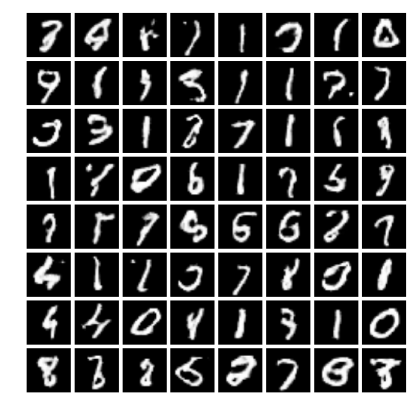
(a) $K=1$

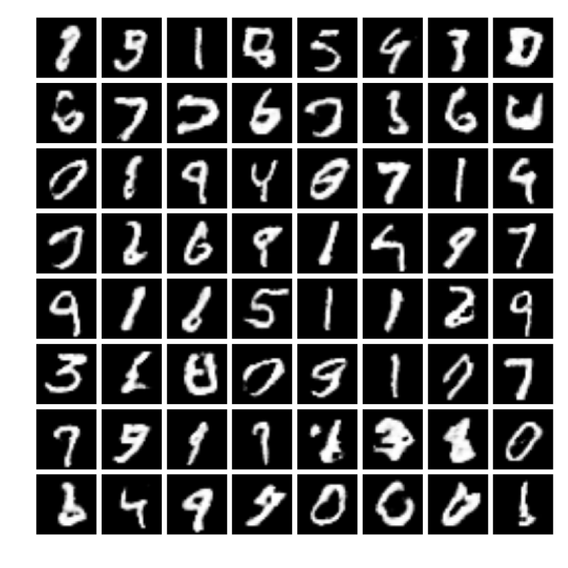
(b) $K=2$

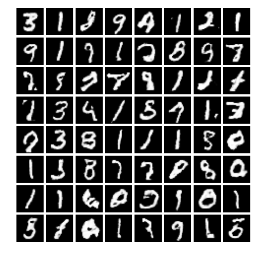
(c) $K=5$

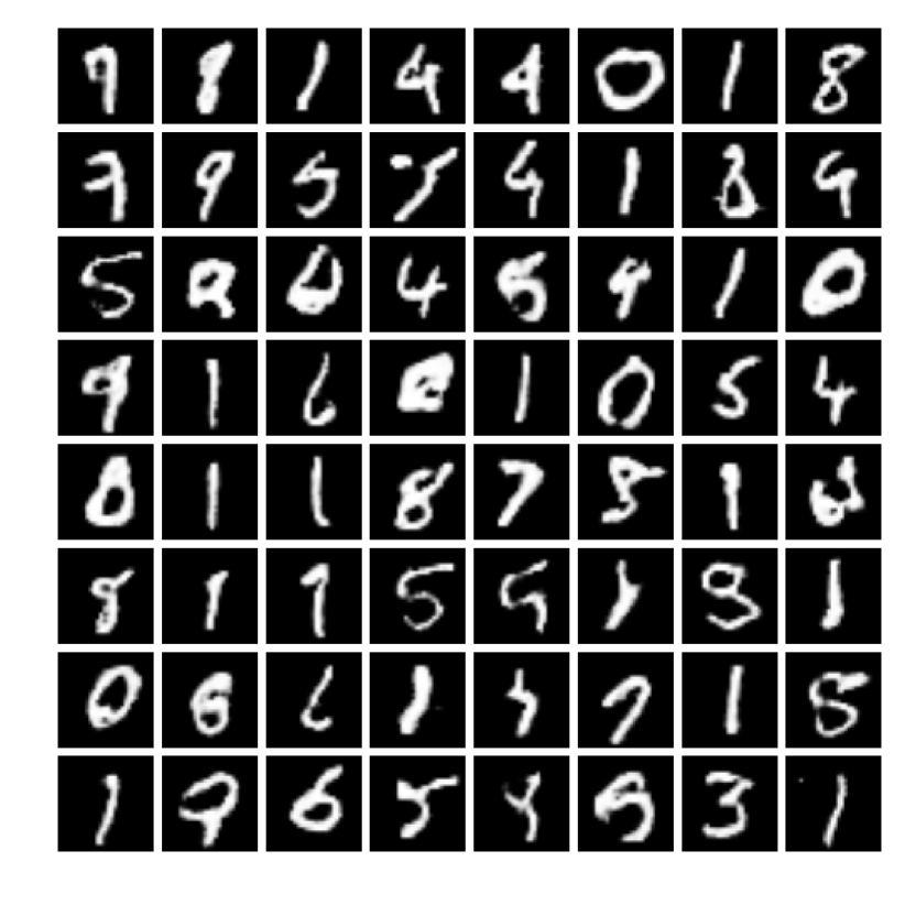
(d) $K=10$

Figure 7: MNIST images generated using GAN after 10000 iterations, trained with $K=1,2,5,10$.

We also trained GANs to generate MNIST images with the $K$-beam method. The objective function is the same as the MoG experiments, but the generator $G$ and the discriminator networks $D$ are more complex as shown in Table 1(b).

The networks are trained with the batch size of 128 using the Adam optimizer with the learning rate of $10^{-3}$.

Fig. 7 shows typical training results for $K=1,2,5,10$ and $J=1$. Images generated with a larger $K$ look slightly more natural than those with a smaller $K$. However, an important difference is that GAN training often fails to converge to a good solution due to “mode collapsing” (Nagarajan & Kolter, 2017) when $K$ is small, as observed by an abrupt change in the cost function during optimization. The mode collapsing rarely happens with larger $K$’s such as $K$=10 with GAN-MNIST. This difference in stability is not directly observable by qualitatively comparing the best generated images from each setting, but it can be measured objectively by average convergence and variance as shown in the figures of the main paper.

Table 1: Generator and discriminator networks for GAN-MNIST

(a) Generator

Type	Size
Input	input dim=10
Fully connected	hidden nodes=7x7x64, ReLU
Conv transpose	filter size=5x5x32, ReLU
Conv transpose	filter size=5x5x1
Sigmoid	output dim=28x28x1

(b) Discriminator

Type	Size
Input	input dim=28x28x1
Conv	filter size=5x5x16, ReLU
Max pool	size=2x2, stride=2x2
Conv	filter size=5x5x32, ReLU
Max pool	size=2x2, stride=2x2
Fully connected	hidden nodes=50, ReLU
Fully connected	output dim=2

References

- Arjovsky et al. (2017) Arjovsky, M., Chintala, S., and Bottou, L. Wasserstein gan. arXiv preprint arXiv:1701.07875, 2017.
- Arrow et al. (1958) Arrow, K. J., Hurwicz, L., Uzawa, H., and Chenery, H. B. Studies in linear and non-linear programming. Stanford University Press, 1958.
- Boyd et al. (2003) Boyd, S., Xiao, L., and Mutapcic, A. Subgradient methods. lecture notes of EE392o, Stanford University, Autumn Quarter, 2003.
- Brückner & Scheffer (2011) Brückner, M. and Scheffer, T. Stackelberg games for adversarial prediction problems. In Proceedings of the 17th ACM SIGKDD international conference on Knowledge discovery and data mining, pp. 547–555. ACM, 2011.
- Chambolle & Pock (2011) Chambolle, A. and Pock, T. A first-order primal-dual algorithm for convex problems with applications to imaging. Journal of mathematical imaging and vision, 40(1):120–145, 2011.
- Correa & Lemaréchal (1993) Correa, R. and Lemaréchal, C. Convergence of some algorithms for convex minimization. Mathematical Programming, 62(1):261–275, 1993.
- Danskin (1967) Danskin, J. M. The theory of max-min and its application to weapons allocation problems. Springer, 1967.
- Dem’janov (1968) Dem’janov, V. F. Algorithms for some minimax problems. Journal of Computer and System Sciences, 2(4):342–380, 1968.
- Dem’yanov & Malozemov (1971) Dem’yanov, V. F. and Malozemov, V. N. On the theory of non-linear minimax problems. Russian Mathematical Surveys, 26(3):57–115, 1971.
- Dem’yanov & Malozemov (1974) Dem’yanov, V. F. and Malozemov, V. N. Introduction to minimax. John Wiley & Sons, 1974.
- Dem’yanov & Pevnyi (1972) Dem’yanov, V. F. and Pevnyi, A. B. Numerical methods for finding saddle points. USSR Computational Mathematics and Mathematical Physics, 12(5):11–52, 1972.
- Durugkar et al. (2016) Durugkar, I., Gemp, I., and Mahadevan, S. Generative multi-adversarial networks. arXiv preprint arXiv:1611.01673, 2016.
- Edwards & Storkey (2015) Edwards, H. and Storkey, A. Censoring representations with an adversary. arXiv preprint arXiv:1511.05897, 2015.
- Ganin & Lempitsky (2015) Ganin, Y. and Lempitsky, V. Unsupervised domain adaptation by backpropagation. In Proceedings of the 32nd International Conference on Machine Learning (ICML-15), pp. 1180–1189, 2015.
- Globerson & Roweis (2006) Globerson, A. and Roweis, S. Nightmare at test time: robust learning by feature deletion. In Proceedings of the 23rd international conference on Machine learning, pp. 353–360. ACM, 2006.
- Golshtein (1972) Golshtein, E. Generalized gradient method for finding saddlepoints. Matekon, 10(3):36–52, 1972.
- Goodfellow et al. (2014) Goodfellow, I., Pouget-Abadie, J., Mirza, M., Xu, B., Warde-Farley, D., Ozair, S., Courville, A., and Bengio, Y. Generative adversarial nets. In Advances in Neural Information Processing Systems, pp. 2672–2680, 2014.
- Hamm (2015) Hamm, J. Preserving privacy of continuous high-dimensional data with minimax filters. In International Conference on Artificial Intelligence and Statistics (AISTATS), pp. 324–332, 2015.
- Hamm (2017) Hamm, J. Minimax filter: learning to preserve privacy from inference attacks. The Journal of Machine Learning Research, 18(1):4704–4734, 2017.
- He & Yuan (2012) He, B. and Yuan, X. Convergence analysis of primal-dual algorithms for a saddle-point problem: From contraction perspective. SIAM Journal on Imaging Sciences, 5(1):119–149, 2012.
- Hiriart-Urruty & Lemaréchal (2001) Hiriart-Urruty, J.-B. and Lemaréchal, C. Fundamentals of convex analysis. Springer, 2001.
- Maistroskii (1977) Maistroskii, D. Gradient methods for finding saddle points. Matekon, 14(1):3–22, 1977.
- Mescheder et al. (2017) Mescheder, L., Nowozin, S., and Geiger, A. The numerics of gans. In Advances in Neural Information Processing Systems, pp. 1823–1833, 2017.
- Nagarajan & Kolter (2017) Nagarajan, V. and Kolter, J. Z. Gradient descent gan optimization is locally stable. In Advances in Neural Information Processing Systems, pp. 5591–5600, 2017.
- Nedić & Ozdaglar (2009) Nedić, A. and Ozdaglar, A. Subgradient methods for saddle-point problems. Journal of optimization theory and applications, 142(1):205–228, 2009.
- Nowozin et al. (2016) Nowozin, S., Cseke, B., and Tomioka, R. f-gan: Training generative neural samplers using variational divergence minimization. arXiv preprint arXiv:1606.00709, 2016.
- Roth et al. (2017) Roth, K., Lucchi, A., Nowozin, S., and Hofmann, T. Stabilizing training of generative adversarial networks through regularization. In Advances in Neural Information Processing Systems, pp. 2015–2025, 2017.
- Saatci & Wilson (2017) Saatci, Y. and Wilson, A. G. Bayesian gan. In Advances in neural information processing systems, pp. 3622–3631, 2017.
- Salmon (1968) Salmon, D. Minimax controller design. IEEE Transactions on Automatic Control, 13(4):369–376, 1968.
- Uehara et al. (2016) Uehara, M., Sato, I., Suzuki, M., Nakayama, K., and Matsuo, Y. Generative adversarial nets from a density ratio estimation perspective. arXiv preprint arXiv:1610.02920, 2016.
- Uzawa (1958) Uzawa, H. Iterative methods in concave programming. In Arrow, K., Hurwicz, L., and Uzawa, H. (eds.), Studies in linear and non-linear programming, chapter 10, pp. 154–165. Stanford University Press, Stanford, CA, 1958.
- v. Neumann (1928) v. Neumann, J. Zur theorie der gesellschaftsspiele. Mathematische annalen, 100(1):295–320, 1928.
- Zabotin (1988) Zabotin, I. A subgradient method for finding a saddle point of a convex-concave function. Issled. Prikl. Mat, 15:6–12, 1988.