On seeking efficient Pareto optimal points in multi-player minimum cost flow problems with application to transportation systems

Abstract

In this paper, we propose a multi-player extension of the minimum cost flow problem inspired by a transportation problem that arises in modern transportation industry. We associate one player with each arc of a directed network, each trying to minimize its cost function subject to the network flow constraints. In our model, the cost function can be any general nonlinear function, and the flow through each arc is an integer. We present algorithms to compute efficient Pareto optimal point(s), where the maximum possible number of players (but not all) minimize their cost functions simultaneously. The computed Pareto optimal points are Nash equilibriums if the problem is transformed into a finite static game in normal form.

1 Introduction

In recent years, product transportation systems are increasingly being dominated by retailers such as Amazon, Alibaba, and Walmart, who utilize e-commerce solutions to fulfill customer supply chain expectations (Turban et al., 2017; Galloway, 1998; Li, 2014; Mendez et al., 2017). In the supply chain strategy of these retailers, products located at different warehouses are shipped to geographically dispersed retail centers by different transportation organizations. These transportation organizations (carriers) compete among themselves and transport goods between warehouses and retail centers over multiple transportation links. For example, Amazon uses FedEx, UPS (United Parcel Service), AAR (Association of American Railroads), and other competing organizations to provide transportation services (Laseter and Rabinovich, 2011, Chapter 11).

Product shipment from a warehouse to a retail center requires contracting multiple competing carriers, e.g., a common shipment may comprise of (i) a trucking shipment from the warehouse to a railhead provided by FedEx, then (ii) a rail shipment provided by AAR, and finally (iii) a trucking shipment from the rail yard to the retail center provided by UPS. It is common that different competing carriers operate over the same transportation link, e.g., both FedEx and UPS provide trucking shipment services for Amazon over the same transportation link (Li, 2014, Section 9.1). The goal of each carrier is to maximize its profit (minimize its cost). So a relevant question in this regard is how to determine a good socially-optimal solution for the competing carriers.

We can formulate the multi-carrier transportation setup described above as a multi-player extension of the well-known minimum cost flow problems. The transportation setup can be modeled by a directed network, where a warehouse is a supply node and a retail center is a demand node. A transportation link is an arc, and a carrier (e.g., FedEx, UPS) in charge of transporting products over that transportation link is a player. The products transported over the directed network are modeled as the flow through the network, and customer supply chain expectations can be modeled as mass-balance constraints. Each of the carriers is trying to maximize its profit by maximizing the total number of products that it transports. Carriers are competing for a limited resource, namely the total number of products to be transported. Note that one carrier making the maximum profit may impact the other carriers in a negative manner and even violate customer supply chain expectations. Our goal is to define a socially-optimal solution concept in this setup and to provide algorithms to calculate such a solution.

The problem above can be generalized as a multi-player minimum cost flow problem (Gupta and Pavel, 2016). We associate one player with one arc of the directed and connected network graph. Parallel arcs between two nodes denote two competing carriers over the same transportation link. Each of the players is trying to minimize its cost function, subject to the network flow constraints. The flow through each arc is taken to be an integer. This assumption incurs no significant loss of generality because by suitable scaling we can use the integer model to obtain a real-valued flow vector to any desired degree of accuracy. Naturally, defining an efficient solution concept is of interest in such a problem setup.

The unambiguously best choice would be a utopian vector optimal solution, which minimizes all the objectives simultaneously. However, this is unlikely to exist in practice (Boyd and Vandenberghe, 2004, page 176). A generic Pareto optimal point, where none of the objective functions can be improved without worsening some of the other objective values, is a better solution concept. However, there can be numerous such generic Pareto optimal points, many of which would be poor in quality or efficiency (Boyd and Vandenberghe, 2004, Section 4.7.5). In this paper, we investigate an efficient Pareto optimal point (Miettinen, 2012, Section 2.2) as a good compromise solution that finds a balance between the utopian vector optimality and the generic Pareto optimality. We present algorithms to compute an efficient Pareto optimal point, i.e., a Pareto optimal point where the maximum possible (but not all) number of players minimize their cost functions simultaneously.

Related work.

  The classic version of the minimum cost flow problem has a linear cost function for which polynomial time algorithms exist (Ahuja et al., 1993, Chapter 10), even when the network structure (e.g., nodes and arcs) is subject to uncertainty (Bertsimas et al., 2013). The polynomial runtime can be improved to a linear runtime when the minimum cost flow problem has a special structure (Vaidyanathan and Ahuja, 2010). However, for nonlinear cost functions, results exist for very specific cases, and no work seems to exist for arbitrary nonlinear functions. The most commonly used nonlinear cost function is the fixed charge function, where the cost on the arc is $0$ if the flow is zero and affine otherwise. Network flow problems with fixed charge costs are studied in (Magnanti and Wong, 1984; Graves and Orlin, 1985; Daskin, 2011), where the integrality condition on the flow is not considered. Minimum cost flow problems with concave cost functions are studied in (Feltenmark and Lindberg, 1997; Yaged, 1971; He et al., 2015; Tuy et al., 1995; Fontes et al., 2006). Minimum cost flow problems with piece-wise linear cost functions is investigated in (Zangwill, 1968; Jorjani and Lamar, 1994; Gamarnik et al., 2012). A dynamic domain contraction algorithm for nonconvex piece-8wise linear network flow problems is proposed in Kim and Pardalos (2000). A particle swarm optimization based hybrid algorithm to solve the minimum concave cost network flow problem is investigated in Yan et al. (2011). Finding Pareto optimal points in multi-objective network flow problem with integer flows has been limited so far to linear cost functions and two objectives (Raith and Ehrgott, 2009; Lee and Pulat, 1993; Eusébio and Figueira, 2009; Hernández et al., 2011). A multi-player minimum cost flow problem with nonconvex cost functions is explored in (Gupta and Pavel, 2016). Integer multi-commodity flow problems are investigated in (Barnhart et al., 1996; Brunetta et al., 2000; Ozdaglar and Bertsekas, 2004); the underlying problems are optimization problems in these papers.

Contributions.

  In this paper, we propose an extension of the minimum cost flow problem to a multi-player setup and construct algorithms to compute efficient Pareto optimal solutions. Our problem can be interpreted as a multi-objective optimization problem (Boyd and Vandenberghe, 2004, Section 4.7.5) with the objective vector consisting of a number of univariate general nonlinear cost functions subject to the network flow constraints and integer flows. In comparison with existing literature, we do not require the cost function to be of any specific structure. The only assumption on the cost functions is that they are proper. In contrast to relevant works in multi-objective network flow problems, our objective vector has an arbitrary number of components; however, each component is a function of a decoupled single variable. We extend this setup to a problem class that is strictly larger than, but that contains the network flow problems. We develop our algorithms for this larger class.

We show that, although in its original form the problem has coupled constraints binding every player, there exists an equivalent variable transformation that decouples the optimization problems for a maximal number of players. Solving these decoupled optimization problems can potentially lead to a significant reduction in the number of candidate points to be searched. We use the solutions of these decoupled optimization problems to reduce the size of the set of candidate efficient Pareto optimal solutions even further using algebraic geometry. Then we present algorithms to compute efficient Pareto optimal points that depend on a certain semi-algebraic set being nonempty. We also present a penalty based approach applicable when that semi-algebraic set is empty; such an approach can be of value to network administrators and policy makers. To the best of our knowledge, our methodology is novel. The computed efficient Pareto optimal point has some desirable properties: (i) it is a good compromise solution between the utopian vector optimality and the generic Pareto optimality, and (ii) it is a Nash equilibrium if we convert our setup into a finite static game in normal form.

The rest of the paper is organized as follows. Section 1 presents notation and notions used in the paper. Section 2 describes the problem for directed networks and the extension to a strictly larger class. In Section 3, we transform the problem under consideration into decoupled optimization problems for a number of players and reformulate the optimization problems for the rest of the players using consensus constraints. Section 4 presents algorithms for computing efficient Pareto optimal points for our problem if a certain semi-algebraic set is nonempty. Section 5 discusses a penalty based approach if the semi-algebraic set is empty. Section 6 presents an illustrative numerical example of our methodology in a transportation setup. Finally, in Section 7 we present some concluding remarks regarding our methodology. Proofs are provided in the Appendix.

Notation and notions.

We denote the sets of real numbers, integers, and natural numbers by $\mathbf{R}$, $\mathbf{Z}$, and $\mathbf{N}$, respectively. The $i$th column, $j$th row, and $(i,j)$th component of a matrix $A\in\mathbf{R}^{m\times n}$ is denoted by $A_{i}$, $a_{j}^{T}$, and $a_{ij}$, respectively. The submatrix of a matrix $A\in\mathbf{R}^{m\times n}$, which constitutes of its rows $r_{1},r_{1}+1,\ldots,r_{2}$ and columns $c_{1},c_{1}+1,\ldots,c_{2}$, is denoted by $A_{[r_{1}:r_{2},c_{1}:c_{2}]}\in\mathbf{R}^{(r_{2}-r_{1}+1)\times(c_{2}-c_{1}+1)}$. If we make two copies of a vector $x\in\mathbf{R}^{n}$, then the copies are denoted by $x^{(1)}$ and $x^{(2)}$. By $I_{i,j}\in\mathbf{R}^{n\times n}$, we denote a matrix that has a $1$ on its $(i,j)$th position and $0$ everywhere else. If $C$ and $D$ are two nonempty sets, then $C+D=\{x+y\mid x\in C,y\in D\}$. If $A\in\mathbf{R}^{m\times n}$ is a matrix and $C$ is a nonempty set containing $n$-dimensional points, then $AC=\{Ax\mid x\in C\}$. The set of consecutive integers from 1 to $n$ is denoted by $[n]=\{1,2,\ldots,n\}$ and $m$ to $n$ is denoted by $[m:n]=\{m,m+1,\ldots,n\}$. If we have two vectors $x,y\in\mathbf{R}^{n}$, then $x\succeq y$ means

$$\left(\forall i\in[n]\right)\quad x_{i}\geq y_{i},$$

and we write $x-y\in\mathbf{R}_{+}^{n}$. Depending on the context, $0$ can represent the scalar zero, a column vector of zeros, or a matrix with all the entries zero, e.g., if we say $x\in\mathbf{R}^{n}$ and $x=0$, then $0$ represents a column vector of $n$ zeros. On the other hand, if we say $A\in\mathbf{R}^{m\times n}$ and $A=0$, then $0$ represents a matrix of $m$ rows and $n$ columns with all entries zero.

Consider a standard form polyhedron $\{x\in\mathbf{R}^{n}\mid Ax=b,x\succeq 0\}$, where $A\in\mathbf{R}^{m\times n}$ is a full row rank matrix, and $b\in\mathbf{R}^{m}$. A basis matrix of this polyhedron is constructed as follows. We pick $m$ linearly independent columns of $A$ and construct the $m\times m$ invertible square submatrix out of those columns; the resultant matrix is called a basis matrix. The concept of basis matrix is pivotal in simplex algorithm, which is used to solve linear programming problem. Suppose we have a polyhedron defined by linear equality and inequality constraints in $\mathbf{R}^{n}$. Then $\tilde{x}\in\mathbf{R}^{n}$ is called a basic solution of the polyhedron, if all the equality constraints are active at $\tilde{x}$, and out of all the active constraints (both equality and inequality) that are active at $\tilde{x}$, there are $n$ of them that are linearly independent.

2 Problem statement

Let $G=(\mathcal{\mathcal{M}},\mathcal{A})$ be a directed connected graph associated with a network, where $\mathcal{M}=[m+1]$ is the set of nodes, and $\mathcal{A}=[n]$ is the set of (directed) arcs. With each arc $j\in\mathcal{A}$, we associate one player, which we call the $j$th player. The variable controlled by the $j$th player is the nonnegative integer flow on arc $j$, denoted by $x_{j}\in\mathbf{Z}$. Each player is trying to minimize a proper cost function $f_{j}:\mathbf{Z}\to\mathbf{R}$, subject to the network flow constraints. We assume each of the cost functions is proper, i.e., for all $i\in[n]$ we have $-\infty\not\not\in f_{i}(\mathbf{Z}),$ and $\textrm{dom}f_{i}=\{x_{i}\in\mathbf{Z}^{n}\mid f_{i}(x_{i})<+\infty\}\neq\emptyset.$ There is an upper bound $u_{j}$, which limits how much flow the $j$th player can carry through arc $j$. Without any loss of generality, we take the lower bound on every arc to be $0$ (Ahuja et al., 1993, Page 39). The supply or demand of flow at each node $i\in\mathcal{M}$ is denoted by $b_{i}$. If $b_{i}>0$, then $i$ is a supply node; if $b_{i}<0$, then $i$ is a demand node with a demand of $-b_{i}$, and if $b_{i}=0$, then $i$ is a trans-shipment node. We allow parallel arcs to exist between two nodes.

In any minimum cost flow problem there are three types of constraints.

(i) Mass balance constraint. The mass balance constraint states that for any node, the outflow minus inflow must equal the supply/demand of the node. We describe the constraint using the node-arc incidence matrix. Let us fix a particular ordering of the arcs, and let $x\in\mathbf{Z}^{n}$ be the resultant vector of flows. First, we define the augmented node-arc incidence matrix $\tilde{A}$, where each row corresponds to a node, and each column corresponds to an arc. The symbol $\tilde{a}_{ij}$ denotes the $(i,j)$th entry of $\tilde{A}$ that corresponds to the $i$th node and the $j$th arc; $\tilde{a}_{ij}$ is $1$ if $i$ is the start node of the $j$th arc, $-1$ if $i$ is the end node of the $j$th arc, and $0$ otherwise. Note that parallel arcs will correspond to different columns with same entries in the augmented node-arc incidence matrix. So every column of $\tilde{A}$ has exactly two nonzero entries, one equal to $1$ and one equal to $-1$ indicating the start node and the end node of the associated arc. Denote, $\tilde{b}=(b_{1},\ldots,b_{m},b_{m+1})$. Then in matrix notation, we write the mass balance constraint as: $\tilde{A}x=\tilde{b}.$ The sum of the rows of $\tilde{A}$ is equal to zero vector, so one of the constraints associated with the rows of the linear system $\tilde{A}x-\tilde{b}$ is redundant, and by removing the last row of the linear system, we can arrive at a system, $Ax=b,$ where $A=\tilde{A}_{[1:m,1:n]}$ is the node-arc incidence matrix, and $b=\tilde{b}_{[1:m]}$. The vector $b$ is also called the resource vector. Now $A$ is a full row rank matrix under the assumption of $G$ being connected and $\sum_{i\in\mathcal{N}}b_{i}=0$ (Bertsimas and Tsitsiklis, 1997, Corollary 7.1).

(ii) Flow bound constraint. The flow on any arc must satisfy the lower bound and capacity constraints, i.e., $0\preceq x\preceq u$. The flow bound constraint can often be relaxed or omitted in practice (Boyd and Vandenberghe, 2004, pages 550-551). In such cases, the flow direction is flexible, and overflow is allowed subject to a suitable penalty.

(iii) Integrality constraint. The flow on any arc is integer-valued, i.e., $x\in\mathbf{Z}^{n}$. This does not incur a significant loss of generality (see Remark 1 below).

So the constraint set, which we denote by $P$ can be written as,

$$P= \left\{x\in\mathbf{Z}^{n}\mid Ax=b,0\preceq x\preceq u\right\},$$ (1)

and the subset of $P$ containing only the equality constraints is denoted by $Q$, i.e.,

$$Q=\left\{x\in\mathbf{Z}^{n}\mid Ax=b\right\}.$$ (2)

Consider a set of players denoted by $[n]$. The decision variable controlled by the $i$th player is $x_{i}\in\mathbf{Z}$, i.e., each player has to take an integer-valued action. The vector formed by all the decision variables is denoted by $x=(x_{1},x_{2},\ldots,x_{n})\in\mathbf{Z}^{n}$. By $x_{-i}\in\mathbf{Z}^{n-1}$, we denote the vector formed by all the players decision variables except $i$th player’s decision variable. To put emphasis on the $i$th player’s variable we sometimes write $x$ as $(x_{i},x_{-i})$. Each player has a cost function $f_{i}(x_{i}):\mathbf{Z}\to\mathbf{R}$, which depends on its variable $x_{i}$. The goal of the $i$th player for $i\in[n]$, given other players’ strategies $x_{-i}\in\mathbf{Z}^{n-1}$, is to solve the minimization problem

$$\begin{aligned} &\text{minimize}_{x_{i}}&&f_{i}\left(x_{i}\right)\\ &\text{subject to}&&A_{i}x_{i}+\sum_{j=1,j\neq i}^{n}A_{j}x_{j}=b\\ &&&0\preceq(x_{i},x_{-i})\preceq u\\ &&&x\in\mathbf{Z}^{n}.\end{aligned}$$ (3)

Our objective is to calculate efficient Pareto optimal points for the problem. We define vector optimal points first, then Pareto optimal point, and finally efficient Pareto optimal point.

Definition 1

(Vector optimal point) In problem (3), a point $x^{\textrm{vo}}\in P$ is vector optimal if it satisfies the following:

$$\left(\forall\tilde{x}\in P\right)\left(\forall i\in[n]\right)\quad f_{i}(\tilde{x}_{i})\geq f_{i}(x_{i}^{\textrm{vo}}).$$

Definition 2

(Pareto optimal point) In problem (3), a point $x^{\textrm{po}}\in P$ is Pareto optimal if it satisfies the following: there does not exist another point $\tilde{x}\in P$ such that

$$\left(\forall i\in[n]\right)\quad f_{i}(\tilde{x}_{i})\leq f_{i}(x_{i}^{\textrm{po}}),$$ (4)

with at least one index $j\in[n]$ satisfying $f_{j}(\tilde{x}_{j})<f_{j}(x_{j}^{\textrm{po}})$.

Definition 3

(Efficient Pareto optimal point) In problem (3), a point $x^{*}$ is an efficient Pareto optimal solution, if it is Pareto optimal and it achieves partial vector optimality over a maximal subset of $[n]$; i.e., $x^{*}$ satisfies (4) and the set $\mathcal{S}\subseteq[n]$ that satisfies

$$\left(\forall\tilde{x}\in P\right)\left(\forall i\in\mathcal{S}\right)\quad f_{i}(\tilde{x}_{i})\geq f_{i}(x_{i}^{*}),$$

is maximal.

Remark 1

In our model, we have taken the flow through any arc of the network to be an integer. However this assumption does not incur a significant loss of generality because we can use our integer model to obtain a real valued Pareto optimal solution to an arbitrary degree of accuracy by using the following scaling technique (Ahuja et al., 1993, page 545). Suppose we want a real valued Pareto optimal solution $x^{*}$. Such a real valued Pareto optimal solution corresponds to a modified version of problem (3) with the last constraint being changed to $x\in\mathbf{R}^{n}.$ In practice, we always have an estimate of how many points after the decimal point we need to consider. So in the modified problem we substitute each $x_{i}$ for $i\in[n]$ with $y_{i}/\alpha$, where $y_{i}\in\mathbf{Z}$, and $\alpha$ is chosen depending on the desired degree of accuracy (e.g., $\alpha$=$1,000$ or $10,000$ or larger depending on how many points after the decimal point we are interested in). Then we proceed with our methodology described in the subsequent sections to compute Pareto optimal solutions over integers. Let $y^{*}$ be one such integer-valued Pareto optimal solution. Then $x^{*}=\left(x_{i}^{*}\right)_{i=1}^{n}=\left(\frac{1}{\alpha}y_{i}^{*}\right)_{i=1}^{n}$ corresponds to a real-valued Pareto optimal solution to the degree of accuracy of $1/\alpha$.

Remark 2

We can formulate our problem as an $n$ person finite static game in normal form (Basar and Olsder, 1995, pages 88-91). In problem (3), a player $i\in[n]$ has a finite but possibly astronomical number of alternatives to choose from the feasible set. Let $\mathfrak{m}_{i}$ be the number of feasible alternatives available to player $i$. Furthermore, define the index set $\mathfrak{M}_{i}=[\mathfrak{m}_{i}]=\{1,\ldots,\mathfrak{m}_{i}\}$ with a typical element of the set designated as $\mathfrak{n}_{i}$, which corresponds to some flow $x_{i}$. If player $1$ chooses a strategy $\mathfrak{n}_{1}\in\mathfrak{M}_{1}$, player $2$ chooses a strategy $\mathfrak{n}_{2}\in\mathfrak{M}_{2}$, and so on for all the other players, then the cost incurred to player $i$ is a single number $\text{$\mathfrak{a}$}_{\mathfrak{n}_{1}\cdots\mathfrak{n}_{n}}^{i}$ that can be determined from problem (3). The ordered tuple of all these numbers (over $i\in[n]$), i.e., $\left(\text{$\mathfrak{a}$}_{\mathfrak{n}_{1}\cdots\mathfrak{n}_{n}}^{1},\text{$\mathfrak{a}$}_{\mathfrak{n}_{1}\cdots\mathfrak{n}_{n}}^{2},\ldots,\text{$\mathfrak{a}$}_{\mathfrak{n}_{1}\cdots\mathfrak{n}_{n}}^{n}\right)$, constitutes the corresponding unique outcome of the game. For a strategy $\left(\mathfrak{n}_{1}\cdots\mathfrak{n}_{n}\right)$ that violates any of the constraints in problem (3), the cost is taken as $+\infty$. Players make their decisions independently, and each player unilaterally seeks the minimum possible loss, of course by also taking into account the possible rational and feasible choices of the other players. The noncooperative Nash equilibrium solution concept within the context of this $n$-person game can be described as follows.

Definition 4

(Noncooperative Nash equilibrium) (Basar and Olsder, 1995, page 88) An $n$-tuple of strategies $\left(\mathfrak{n}_{1}^{{\rm Nash}},\ldots,\mathfrak{n}_{n}^{{\rm Nash}}\right)$ with $\mathfrak{n}_{i}^{{\rm Nash}}\in\mathfrak{M}_{i}$ for all $i\in[n]$, is said to constitute a noncooperative Nash equilibrium solution for the aforementioned $n$-person nonzero-sum static finite game in normal form if the following $n$ inequalities are satisfied for all $\mathfrak{n}_{i}\in\mathfrak{M}_{i}$ and all $i\in[n]$:

$$\mathfrak{a}^{i,{\rm Nash}}=\text{$\mathfrak{a}$}_{\mathfrak{n}_{1}^{{\rm Nash}}\mathfrak{n}_{2}^{{\rm Nash}}\cdots\mathfrak{n}_{n}^{{\rm Nash}}}^{i}\leq\text{$\mathfrak{a}$}_{\mathfrak{n}_{1}^{{\rm Nash}}\mathfrak{n}_{2}^{{\rm Nash}}\cdots\mathfrak{n}_{i}\cdots\mathfrak{n}_{n}^{{\rm Nash}}}^{i}.$$ (5)

The flow corresponding to $\left(\mathfrak{n}_{1}^{{\rm Nash}},\ldots,\mathfrak{n}_{n}^{{\rm Nash}}\right)$ is denoted by $x^{{\rm Nash}}=\left(x_{1}^{{\rm Nash}},\ldots,x_{n}^{{\rm Nash}}\right)$ and is called the noncooperative Nash equilibrium flow. Here, the $n$-tuple $(\mathfrak{a}^{1,{\rm Nash}},\mathfrak{a}^{2,{\rm Nash}},\ldots,\mathfrak{a}^{n,{\rm Nash}})$ is known as a noncooperative (Nash) equilibrium outcome of the $n$-person game in normal form. Note that the strategy associated with an efficient Pareto optimal solution $x^{*}$ in Definition 3 also satisfies (5) in Definition 4, thus it is a noncooperative Nash equilibrium flow.

We now extend the class of problems that we are going to investigate, which is strictly larger than the class defined by problem (3) and contains it. We will develop our algorithms for this larger class. Everything defined in the previous subsection still holds, and we extend the constraint set $P$ and the equality constraint set $Q$ as follows. The structure of $P$ is still that of a standard form integer polyhedron, i.e., $P=\{x\in\mathbf{Z}^{n}\mid Ax=b,0\preceq x\preceq u\}$, where $A$ is a full row rank matrix, but it may not necessarily be a node-arc incidence matrix only. Denote the convex hull of the points in $P$ by $\mathop{\bf conv}P$. Consider the relaxed polyhedron $\mathop{\bf relaxed}P=\{x\in\mathbf{R}^{n}\mid Ax=b,0\preceq x\preceq u\}$, where we have relaxed the condition of $x$ being an integer-valued vector. We now impose the following assumption.

Assumption 1

For any integer-valued $b$, $\mathop{\bf relaxed}P$ has at least one integer-valued basic solution.

As vertices of a polyhedron are also basic solutions (Bertsimas and Tsitsiklis, 1997, page 50), if $\mathop{\bf conv}P$ and $\mathop{\bf relaxed}P$ share at least one vertex, Assumption 1 will be satisfied. We can see immediately that if $A$ is a node-arc incidence matrix, then $P$ will belong to this class as $\mathop{\bf conv}P=\mathop{\bf relaxed}P$ for network flow problems (Schrijver, 1998, Chapter 19). In other practical cases of interest, the matrix can satisfy Assumption 1, e.g., matrices with upper or lower triangular square submatrices with diagonal entries 1, sparse matrices with $m$ variables appearing only once with coefficients one, etc. Moreover, at the expense of adding slack variables (thus making a larger dimensional problem), we can turn the problem under consideration into one satisfying Assumption 1, though the computational price may be heavy.

In the rest of the paper, whenever we mention (1), (2), and (3), they correspond to this larger class of problems containing the network flow problems, and the full row rank matrix $A$ is associated with this larger class. So the results developed in the subsequent sections will hold for a network flow setup.

Remark 3

Before proceeding any further, we recall that integer programming problems are $\mathcal{NP}$-hard, and even determining the existence of one feasible point in $P$ is $\mathcal{NP}$ hard (Bertsimas and Weismantel, 2005, page 242). So problem (3) is at least as hard.

3 Problem transformation

In this section, we describe how to transform problem (3) into $n-m$ decoupled optimization problems for the last $n-m$ players and how to reformulate the optimization problems for the rest of the players using consensus constraints. These transformation and reformulation are necessary for the development of our algorithms.

3.1 Decoupling optimization problems for the last $n-m$ players

First, we present the following lemma. Recall that, an integer square matrix is unimodular if its determinant is $\pm 1$.

Lemma 1

Assumption 1 holds if and only if we can extract a unimodular basis matrix from $A$.

Without any loss of generality, we rearrange the columns of the matrix $A$ so that the unimodular basis matrix constitutes the first $m$ columns, i.e., if $A=[A_{1}\mid A_{2}\mid\ldots\mid A_{m}\mid A_{m+1}\mid\ldots\mid A_{n}]$, then $\det([A_{1}\mid A_{2}\mid\ldots\mid A_{m}])=\pm 1$, and we reindex the variables accordingly. Let us denote $[A_{1}\mid A_{2}\mid\ldots\mid A_{m}]=B$, so $A=[B\mid A_{m+1}\mid\ldots\mid A_{n}]$. Next we present the following Lemma.

Lemma 2

Let, $C=B^{-1}A$ and $d=B^{-1}b$. Then $C\in\mathbf{Z}^{m\times n}$, $d\in\mathbf{Z}^{m}$, and the sets $Q$ and $P$ (defined in (1) and (2), respectively) have the equivalent representations:

$$Q =\left\{x\in\mathbf{Z}^{n}\mid Cx=d\right\},$$ (6)

$$P =\left\{x\in\mathbf{Z}^{n}\mid Cx=d,0\preceq x\preceq u\right\}.$$ (7)

Before we present the next result, we recall the following definitions and facts. A full row rank matrix $A\in\mathbf{Z}^{m\times n}$ is in Hermite normal form, if it is of the structure $[B|0]$, where $B\in\mathbf{Z}^{m\times m}$ is invertible and lower triangular, and $0$ represents $\{0\}^{m\times n-m}$ (Schrijver, 1998, Section 4.1). Any full row rank integer matrix can be brought into the Hermite normal form using elementary integer column operations in polynomial time in the size of the matrix (Bertsimas and Weismantel, 2005, Page 243).

Lemma 3

The matrix $C$, as defined in Lemma 2, can be brought into the Hermite normal form $[I|0]$ by elementary integer column operations, more specifically by adding integer multiple of one column to another column.

Lemma 4

There exists a unimodular matrix $U$ such that $CU=\left[I\mid 0\right]$.

The following theorem is key in transforming the problem into an equivalent form with $m$ decoupled optimization problems for players $m+1,m+2,\ldots,n$.

Theorem 3.1

The constraint set $Q$ defined in (6) is nonempty. Furthermore, any vector $x\in Q$ can be maximally decomposed in terms of a new variable $z\in\mathbf{Z}^{n-m}$ as follows:

$$x\in Q\Leftrightarrow\exists z\in\mathbf{Z}^{n-m}\textrm{ such that }x=\begin{bmatrix}d_{1}-h_{1}^{T}z\\ d_{2}-h_{2}^{T}z\\ \vdots\\ d_{m}-h_{m}^{T}z\\ z_{1}\\ \vdots\\ z_{n-m}\end{bmatrix},$$ (8)

where $d_{i}$ is the $i$th component of $d=B^{-1}b$, and $h_{i}^{T}\in\mathbf{Z}^{1\times n-m}$ is the $i$th row of $B^{-1}A_{[1:m,m+1:n]}$.

We can transform our problem using the new variable $z$. The advantage of this transformation is that for player $m+1,m+2,\ldots,n$, we have decoupled optimization problems. By solving these decoupled problems, we can reduce the constraint set significantly (especially when the number of minimizers for the constraint set are small).

From Theorem 3.1, $x_{i}=z_{i-m}$ for $i\in[m+1:n]$. For problem (3), we can write the optimization problem for any player $m+i$ for $i\in[n-m]$ as follows.

$$\begin{aligned} &\text{minimize}_{z_{i}}&&f_{i}(z_{i})\\ &\text{subject to}&&0\leq z_{i}\leq u_{i}\\ &&&z_{i}\in\mathbf{Z}.\end{aligned}$$ (9)

Each of these optimization problems is a decoupled univariate optimization problem, which can be easily solved graphically. We can optimize over real numbers, find the minimizers of the resultant relaxed optimization problem, determine whether the floor or ceiling of such a minimizer results in the minimum cost, and pick that as a minimizer of the original problem. Solving $n-m$ decoupled optimization problems immediately reduces the constraint set into a much smaller set. Let us denote the set of different optimal solutions for player $m+i$ for $i\in[n-m]$ as $D_{i}=\left\{z_{i,1},z_{i,2},\ldots,z_{i,p_{i}}\right\}$ sorted from smaller to larger, where $p_{i}$ is the total number of minimizers. Define, $D=\bigtimes_{i=1}^{n-m}D_{i}$. Note that $D\neq\emptyset$ .

3.2 Consensus reformulation for the first $m$ players

In this section, we transform the optimization problems for the first $m$ players using (8) and consensus constraints. Consider the optimization problems for the first $m$ players in variable $z$, which have coupled costs due to (8). We deal with the issue by introducing consensus constraints (Parikh and Boyd, 2013, Section 5.2). We provide each player $i\in[m]$ with its own local copy of $z$, denoted by $z^{(i)}\in\mathbf{Z}^{n-m}$, which acts as its decision variable. This local copy has to satisfy the following conditions. First, using (8) for any $i\in[m]$, $x_{i}=d_{i}-h_{i}^{T}z^{(i)}$. The copy $z^{(i)}$ has to be in consensus with the rest of the first $m$ players, i.e., $z^{(i)}=z^{(j)}$ for all $j\in[m]\setminus\{i\}$. Second, the copy $z^{(i)}$ has to satisfy the flow bound constraints, i.e., $0\leq d_{i}-h_{i}^{T}z^{(i)}\leq u_{i}$ for all $i\in[m]$. Third, for the last $n-m$ players $z_{i}\in D_{i}$, as obtained from the solutions of the decoupled optimization problems (9), so $z^{(i)}$ has to be in $D$, i.e., for all $i\in[m]$ we have

$$z^{(i)}=z\in D\Leftrightarrow\left(\forall j\in[n-m]\right)z_{j}^{(i)}\in D_{j}.$$

Combining the aforementioned conditions, for all $i\in[m]$, the $i$th player’s optimization problem in variable $z^{(i)}$ can be written as:

$$\begin{aligned} &\text{minimize}_{z^{(i)}}&&\bar{f}_{i}\left(z^{(i)}\right)=f_{i}(d_{i}-h_{i}^{T}z^{(i)})\\ &\text{subject to}&&z^{(i)}=z^{(j)},\quad j\in[m]\setminus\{i\}\\ &&&0\leq d_{i}-h_{i}^{T}z^{(i)}\leq u_{i}\\ &&&z_{j}^{(i)}\in D_{j},\quad j\in[n-m].\end{aligned}$$ (10)

An integer linear inequality constraint $\alpha\leq v\leq\beta,$ where $\alpha,\beta,v\in\mathbf{Z}$, is equivalent to $v\in\{\alpha,\alpha+1,\ldots,\beta\}\Leftrightarrow(v-\alpha)(v-\alpha-1)\cdots(v-\beta)=0$. Using this fact, we write the last two constraints in (10) in polynomial forms as follows.

$$q_{i}(z^{(i)})=(d_{i}-h_{i}^{T}z^{(i)})(d_{i}-h_{i}^{T}z^{(i)}-1)\cdots(d_{i}-h_{i}^{T}z^{(i)}-u_{i})=0,$$ (11)

$$r_{j}(z^{(i)})=(z_{j}^{(i)}-z_{j,1})(z_{j}^{(i)}-z_{j,2})\ldots(z_{j}^{(i)}-z_{j,p_{i}})=0,\quad\quad j\in[n-m].$$ (12)

Hence for all $i\in[m]$ any feasible $z^{(i)}$ for problem (10) comes from the following set:

$$\mathcal{F} = \bigcap_{k=1}^{m}\{z\in\mathbf{Z}^{n-m}\mid q_{k}(z)=0,\textrm{and}\left(\forall j\in[n-m]\right)\quad r_{j}(z)=0\}$$ (13)

$$= \{z\in\mathbf{Z}^{n-m}\mid\left(\forall k\in[m]\right)\;q_{k}(z)=0,\textrm{and}\left(\forall j\in[n-m]\right)\;r_{j}(z)=0\}.$$

In (13), the intersection in the first line ensures that the consensus constraints are satisfied, and the second line just expands the first. So the optimization problem (10) is equivalent to

$$\begin{aligned} &\textrm{minimize}_{z^{(i)}}&&\bar{f}_{i}\left(z^{(i)}\right)\\ &\text{subject to}&&z^{(i)}\in\mathcal{F},\end{aligned}$$ (14)

for $i\in[m]$. Thus each of these players is optimizing over a common constraint set $\mathcal{F}$. So finding the points in $\mathcal{F}$ is of interest, which we discuss next.

4 Algorithms

In this section, first, we review some necessary background on algebraic geometry, and then we present a theorem to check if $\mathcal{F}$ is nonempty and provide an algorithm to compute the points in a nonempty $\mathcal{F}$. Finally, we present our algorithm to compute efficient Pareto optimal points. In devising our algorithm, we use algebraic geometry rather than integer programming techniques for the following reasons. First, in this way, we are able to provide an algebraic geometric characterization for the set of efficient Pareto optimal solutions for our problem. Second, we can show that this set is nonempty if and only if the reduced Groebner basis (disucussed in Section 4.1 below) of a certain set associated with the problem is not equal to $\{1\}$ (Theorem 4.2). Third, the mentioned result has an algorithmic significance: the reduced Groebner basis can be used to construct algorithms to calculate efficient Pareto optimal points.

4.1 Background on algebraic geometry

A monomial in variables $x=(x_{1},x_{2},\ldots,x_{n})$ is a product of the structure $x^{\alpha}=x_{1}^{\alpha_{1}}\cdots x_{n}^{\alpha_{n}},$ where $\alpha=(\alpha_{1},\ldots,\alpha_{n})\in\mathbf{N}{}^{n}$. A polynomial is an expression that is the sum of a finite number of terms with each term being a monomial times a real or complex coefficient. The set of all real polynomials in $x=(x_{1},\ldots,x_{n})$ with real and complex coefficients are denoted by $\mathbf{R}[x]$ and $\mathbf{C}[x]$, respectively, with the variable ordering $x_{1}>x_{2}>\cdots>x_{n}$. The ideal generated by $f_{1},f_{2},\ldots,f_{m}\in\mathbf{\mathbf{C}}[x]$ is the set

$$\mathbf{ideal}\left\{f_{1},\ldots,f_{m}\right\}=\left\{\sum_{i=1}^{m}h_{i}f_{i}\mid\left(\forall i\in[m]\right)\;h_{i}\in\mathbf{C}[x]\right\}.$$

Consider $f_{1},f_{2},\ldots,f_{s}$ which are polynomials in $\mathbf{C}[x]$. The affine variety $V$ of $f_{1},f_{2},\ldots,f_{m}$ is given by

$$V(f_{1},\ldots,f_{m}) = \left\{x\in\mathbf{C}^{n}\mid\left(\forall i\in[m]\right)\quad f_{i}(x)=0\right\}.$$ (15)

A monomial order on $\mathbf{C}[x_{1},\ldots,x_{n}]$ is a relation, denoted by $\succ$, on the set of monomials $x^{\alpha},\alpha\in\mathbf{N}^{n}$ satisfying the following. First, it is a total order; second, if $x^{\alpha}\succ x^{\beta}$ and $x^{\gamma}$ is any monomial, then $x^{\alpha+\gamma}\succ x^{\beta+\gamma}$; third, every nonempty subset of $\mathbf{N}^{n}$ has a smallest element under $\succ$. We will use lexicographic order, where we say $x^{\alpha}\succ_{\text{lex}}x^{\beta}$ if and only if the left most nonzero entry of $\alpha-\beta$ is positive. Suppose that we are given a monomial order $\succ$ and a polynomial $f(x)=\sum_{\alpha\in S}f_{\alpha}x^{\alpha}$. The leading term of the polynomial with respect to $\succ$, denoted by $\textrm{lt}_{\succ}\left(f\right)$, is that monomial $f_{\alpha}x^{\alpha}$ with $f_{\alpha}\neq 0$, such that $x^{\alpha}\succ x^{\beta}$ for all other monomials $x^{\beta}$ with $f_{\beta}\neq 0$. The monomial $x^{\alpha}$ is called the leading monomial of $f$. Consider a nonzero ideal $I$. The set of the leading terms for the polynomials in $I$ is denoted by $\textrm{lt}_{\succ}\left(I\right)$. Thus $\textrm{lt}_{\succ}\left(I\right)=\left\{cx^{\alpha}\mid\left(\exists f\in I\right)\quad\textrm{lt}_{\succ}(f)=cx^{\alpha}\right\}.$ By $\mathbf{ideal}\left\{\textrm{lt}_{\succ}\left(I\right)\right\}$ with respect to $\succ$, we denote the ideal generated by the elements of $\textrm{lt}_{\succ}\left(I\right)$.

A Groebner basis $G_{\succ}$ of an ideal $I$ with respect to the monomial order $\succ$ is a finite set of polynomials $g_{1},\ldots,g_{t}\in I$ such that $\mathbf{ideal}\left\{\textrm{lt}_{\succ}\left(I\right)\right\}=\mathbf{ideal}\left\{\textrm{lt}_{\succ}\left(g_{1}\right),\ldots,\textrm{lt}_{\succ}\left(g_{t}\right)\right\}.$ A reduced Groebner basis $G_{\textrm{reduced},\succ}$ for an ideal $I$ is a Groebner basis for $I$ with respect to monomial order $\succ$ such that, for any $f\in G_{\textrm{reduced},\succ}$, the coefficient associated with $\textrm{lt}_{\succ}\left(f\right)$ is $1$, and for all $f\in G_{\textrm{reduced},\succ}$, no monomial of $f$ lies in $\mathbf{ideal}\left\{\textrm{lt}_{\succ}\left(G\setminus\{f\}\right)\right\}$. For a nonzero ideal $I$ and given monomial ordering, the reduced Groebner basis is unique (Proposition 6, Cox et al., 2007, Page 92). Suppose $I=\mathbf{ideal}\left\{f_{1},\ldots,f_{m}\right\}\subseteq\mathbf{C}\left[x_{1},\ldots,x_{n}\right]$. Then for any $l\in[n]$, the $l$th elimination ideal for $I$ is defined by $I_{l}=I\cap\mathbf{C}[x_{l+1},\ldots,x_{n}].$ Let $I\subseteq\mathbf{C}\left[x_{1},\ldots,x_{n}\right]$ be an ideal, and let $G$ be a Groebner basis of $I$ with respect to lexicographic order with $x_{1}\succ x_{2}\succ\ldots\succ x_{n}$. Then for every integer $l\in\left\{0,n-1\right\}$, the set $G_{l}=G\cap\mathbf{C}\left[x_{l+1},\ldots,x_{n}\right]$ is a Groebner basis for the $l$th elimination ideal $I_{l}$.

4.2 Nonemptyness of $\mathcal{F}$

We will use the following theorem in proving the results in this section.

Theorem 4.1

(Weak Nullstellensatz (Theorem 1, Cox et al., 2007, page 170)) Consider $f_{1},f_{2},\ldots,f_{s}$ as polynomials in $\mathbf{C}[x_{1},x_{2},\ldots,x_{n}]$. If $V(f_{1},f_{2},\ldots,f_{m})=\emptyset$ (see (15) for definition of $V$), then

$$\mathbf{ideal}\{f_{1},f_{2},\ldots,f_{m}\}=\mathbf{C}[x_{1},x_{2},\ldots,x_{n}].$$

First, we present the following result.

Theorem 4.2

The set $\mathcal{F}$ is nonempty if and only if

$$G_{\textrm{reduced},\succ}\neq\{1\},$$

where $G_{\textrm{reduced},\succ}$ is the reduced Groebner basis of $\mathbf{ideal}\left\{q_{1},\ldots,q_{m},r_{1},\ldots,r_{n-m}\right\}$ with respect to any ordering.

Remark 4

In the proof, we have shown that feasibility of the system (26) in $\mathbf{C}^{n-m}$ is equivalent to its feasibility in $\mathbf{Z}^{n-m}$. So

$$V\left(q_{1},\ldots,q_{m},r_{1},\ldots,r_{n-m}\right)\cap\mathbf{Z}^{n-m}=V\left(q_{1},\ldots,q_{m},r_{1},\ldots,r_{n-m}\right).$$ (16)

If we are interested in just verifying the feasibility of the polynomial system, then calculating a reduced Groebner basis with respect to any ordering suffices. However, if we are interested in extracting the feasible points, then we choose lexicographic ordering as lexicographic ordering allows us to use algebraic elimination theory. There are many computer algebra packages to compute reduced Groebner basis such as Macaulry2, SINGULAR, FGb, Maple, and Mathematica. We now describe how to extract the points in $\mathcal{F}$.

Suppose $G_{\textrm{reduced},\succ}\neq\{1\}$. Naturally, the next question is how to compute points in $\mathcal{F}$? In the next section, we will show that the points in $\mathcal{F}$ are related to the efficient Pareto optimal points that we are seeking. We now briefly discuss systematic methods for extracting $\mathcal{F}$ based on algebraic elimination theory, a branch of computational algebraic geometry. For details on elimination theory, we refer the interested readers to (Cox et al., 2007, Chapter 3). First, we present the following lemma.

Lemma 5

Suppose $G_{\textrm{reduced},\succ}\neq\{1\}$. Then $\mathcal{F}=V\left(G_{\textrm{reduced},\succ_{\textrm{lex}}}\right)\neq\emptyset.$

Algorithm 1 below calculates all the points in $\mathcal{F}$, when $G_{\textrm{reduced},\succ_{\textrm{lex}}}\neq\{1\}.$ Lemma 6 proves its accuracy.

Lemma 6

Algorithm 1 correctly calculates all the points in $\mathcal{F}$, when it is nonempty.

Input: Polynomial system $q_{i}(z)=0$ for $i\in[m]$, and $r_{j}(z)=0$ for $j\in[n-m]$, $G_{\textrm{reduced},\succ_{\textrm{lex}}}\neq\{1\}.$

Output: The set $\mathcal{F}$.

Step

1.

• Calculate the set $G_{n-m-1}=G_{\textrm{reduced},\succ_{\textrm{lex}}}\cap\mathbf{C}\left[z_{n-m}\right],$ which is a Groebner basis of the $(n-m)$th elimination ideal of $\mathbf{ideal}\left\{q_{1},\ldots,q_{m},r_{1},\ldots,r_{n-m}\right\}$ that consists of univariate polynomials in $z_{n-m}$ as an implication of (Cox et al., 2007, page 116, Theorem 2).

• Find the variety of $G_{n-m-1}$, denoted by $V\left(G_{n-m-1}\right),$ which contains the list all possible $z_{n-m}$ coordinates for the points in $\mathcal{F}$.

Step

2.

• Calculate $G_{n-m-2}=G_{\textrm{reduced},\succ_{\textrm{lex}}}\cap\mathbf{C}\left[z_{n-m-1},z_{n-m}\right],$ which is again a Groebner basis of the $(n-m-1)$th elimination ideal of $\mathbf{ideal}\left\{q_{1},\ldots,q_{m},r_{1},\ldots,r_{n-m}\right\}$ and consists of bivariate polynomials in $z_{n-m}$ and $z_{n-m-1}$.

• From Step 1, we already have the $z_{n-m}$ coordinates for the points in $\mathcal{F}$. So by substituting those $|V(G_{n-m-1})|$ values in $G_{n-m-2}$, we arrive at a set of univariate polynomials in $z_{n-m-1}$, which we denote by $\{\bar{G}_{n-m-2}^{(i)}\}_{i=1}^{|V(G_{n-m-1})|}$.

• For all $i=1,2,\ldots,|V(G_{n-m-1})|$, find the variety of $\bar{G}_{n-m-2}^{(i)}$, denoted by $V(\bar{G}_{n-m-2}^{(i)})$, which contains the list all possible $z_{n-m-1}$ coordinates associated with a particular $z_{n-m}\in V(G_{n-m-1})$. We now have all the possible $\left(z_{n-m-1},z_{n-m}\right)$ coordinates of $\mathcal{F}$.

Step

3.

• We repeat this procedure for $G_{n-m-3},G_{n-m-4},\ldots,G_{0}$. In the end, we have set of all points in $\mathcal{F}$.

return $\mathcal{F}$.

Algorithm 1 Extracting the points in $\mathcal{F}$

4.3 Finding efficient Pareto optimal points from $\mathcal{F}$

Suppose $G_{\textrm{reduced},\succ_{\textrm{lex}}}\neq\{1\}$, and using Algorithm 1 we have computed $\mathcal{F}$. We now propose Algorithm 2 and show that the resultant points are Pareto optimal.

Input: The optimization problem (14) for any $i\in[m]$, $\mathcal{F}\neq\emptyset$.

Output: Efficient Pareto optimal solutions for problem (3).

Step

1.

for

$i=1,\ldots,m$

$$X_{i}:=\left\{d_{i}-h_{i}^{T}z^{(i)}\mid z^{(i)}\in\mathcal{F}\right\}=d_{i}-h_{i}^{T}\mathcal{F},$$

$$\left(\forall x_{i}\in X_{i}\right)\quad(X_{i})^{-1}(x_{i}):=\{z^{(i)}\in\mathcal{F}\mid x_{i}=d_{i}-h_{i}^{T}z^{(i)}.\}$$ (17)

end

for

Step

2.

Sort the elements of the $\{X_{i}\}_{i=1}^{m}$s with respect to cardinality of the elements in a descending order. Denote the index set of the sorted set by $\{s_{1},s_{2},\ldots,s_{m}\}$ such that

$$|X|_{s_{1}}\geq|X|_{s_{2}}\geq\cdots\geq|X|_{s_{m}}.$$

Step

3.

for

$i\in[m]$

Solve the univariate optimization problem

$$\begin{aligned} &\mathrm{minimize}_{x_{s_{i}}}&&f_{s_{i}}(x_{s_{i}})\\ &\mathrm{subject\;to}&&x_{s_{i}}\in X_{s_{i}},\end{aligned}$$ (18)

and denote the set of solutions by $X_{s_{i}}^{*}$. Set

$$\mathcal{F}_{s_{i}}^{*} := \bigcup_{x_{s_{i}}\in X_{s_{i}}^{*}}(X_{s_{i}}^{*})^{-1}(x_{s_{i}})\subseteq\mathcal{F},$$ (19)

if

$i\leq m$

$$X_{s_{i+1}}:=\left\{d_{s_{i+1}}-h_{s_{i+1}}^{T}z\mid z\in\mbox{$\mathcal{F}$}_{s_{i}}^{*}\right\}.$$ (20)

end

if

end

for

return $\mathcal{F}_{s_{m}}^{*}.$

Algorithm 2 Computing the set of solutions to problem (14).

We have the following results for Algorithm 2.

Lemma 7

In Algorithm 2, for all $i\in[m-1]$, we have $\mathcal{F}_{s_{i+1}}^{*}\subseteq\mathcal{F}_{s_{i}}^{*}\subseteq\mathcal{F}$ ($\mathcal{F}_{s_{i}}^{*}$ defined in (19)).

Lemma 8

In Algorithm 2, for any $i\in[m]$, $x_{s_{i}}\in X_{s_{i}}^{*}$ (the set $X_{i}^{*}$ is defined in Step 1, 3 of Algorithm 2) if and only if $z^{*}\in\mathcal{F}_{s_{i}}^{*}$. Furthermore, $z^{*}\in\mathcal{F}_{s_{i}}^{*}$ solves the following optimization problem

$$\begin{aligned} &\mathrm{minimize}_{z}&&f_{s_{i}}(d_{s_{i}}-h_{s_{i}}^{T}z)\\ &\mathrm{subject\;to}&&z\in\mathcal{F}_{s_{i-1}}^{*},\end{aligned}$$

for all $i\in[2:m]$.

In Algorithm 2, at no stage can $\mathcal{F}_{s_{i}}^{*}$ get empty.

Lemma 9

Suppose $\mathcal{F}\neq\emptyset$. Then in Algorithm 2, $\mathcal{F}_{s_{i}}^{*}$ is nonempty for any $i\in[m]$.

Theorem 4.3

For any $z^{*}\in\mathcal{F}_{s_{m}}^{*}$,

$$x^{*}=(d_{1}-h_{1}^{T}z^{*},\ldots,d_{m}-h_{m}^{T}z^{*},z_{1}^{*},\ldots,z_{n-m}^{*})$$ (21)

is an efficient Pareto optimal point.

5 A penalty based approach when $\mathcal{F}$ is empty

In the case that $\mathcal{F}$ is empty, we design a penalty based approach to solve a penalized version of problem (14) that can be of use to network administrators and policy makers. First, for $i\in[m]$, using (13), (12), and (11), problem (14) can be written in the following equivalent form:

$$\begin{aligned} &\textrm{minimize}_{z^{(i)}\in D}&&\bar{f}_{i}\left(z^{(i)}\right)\\ &\text{subject to}&&\left(\forall k\in[m]\right)\quad q_{k}(z^{(i)})=0.\end{aligned}$$ (22)

When $\mathcal{F}=\emptyset$, we relate the problem above to a penalized version, which is a standard practice in operations research literature (Bertsekas et al., 2003, Page 278). In this penalized version, we disregard the equality constraints $q_{k}(z^{(i)})=0$ for $k\in[m]$, rather we we augment the cost with a term that penalizes the violation of these equality constraints. So a penalized version of the problem (22) is as follows:

$$\begin{aligned} &\textrm{minimize}_{z^{(i)}}&&\bar{f}_{i}\left(z^{(i)}\right)+\sum_{k=1}^{m}\gamma_{k}p\left(q_{k}(z^{(i)})\right),\\ &\textrm{subject to}&&z^{(i)}\in D.\end{aligned}$$ (23)

where $p:\mathbf{R}\to\mathbf{R}_{+}$ is a penalty function, and $\gamma_{k}$ is a positive penalty parameter. Some common penalty functions are:

• exact penalty: $p:x\mapsto x^{2}$,

• power barrier: $p:x\mapsto|x|$, etc.

We have already shown $D$ to be a nonempty set. From a network point of view, the penalized problem (23) has the following interpretation. For the first $m$ arcs in the directed network under consideration, rather than having a strict flow bound constraint (see the discussion in Section 2), we have a penalty when $x_{i}<0$ or $x_{i}>u_{i}$ for $i\in[m]$. The flow bound constraint is still maintained for $i\in[m+1:n]$. In this regard, the original problem defined by (3) has the following penalized version:

$$\begin{aligned} &\text{minimize}_{x_{i}}&&f_{i}\left(x_{i}\right)+\left({\textrm{penalty for violation of }\atop 0\leq x_{i}\leq u_{i}\textrm{ for player }i\in[m]}\right)\\ &\text{subject to}&&Ax=A(x_{i},x_{-i})=A_{i}x_{i}+\sum_{j=1,j\neq i}^{n}A_{j}x_{j}=b\\ &&&0\leq x_{i}\leq u_{i},\quad i\in[m+1:n]\\ &&&x\in\mathbf{Z}^{n}.\end{aligned}$$ (24)

Problem (24) can be considered as a network flow problem, where flow direction is flexible or overflow is allowed subject to a suitable penalty, which is a quite realistic scenario in practice (Boyd and Vandenberghe, 2004, pages 550-551). With this penalized problem, we can proceed as follows. In the developments of Section 4.3 set:

$$\bar{f}_{i}\left(z^{(i)}\right):=\bar{f}_{i}\left(z^{(i)}\right)+\sum_{k=1}^{m}\gamma_{k}p\left(q_{k}(z^{(i)})\right),$$

$$\mathcal{F}:=D\neq\emptyset,$$

and then apply Algorithm 2, which will calculate efficient Pareto optimal points for the penalized problem (24).

The described penalty scheme can be of use to network administrators and policy makers to enforce a decision making architecture. Such an architecture would allow the players to make independent decisions while ensuring that (i) total amount of flow is conserved in the network by maintaining the mass balance constraint, (ii) the flow bound constraint is strictly enforced for the last $n-m$ players and is softened for the first $m$ players by imposing penalty, and yet (iii) an efficient Pareto optimal point for the penalized problem can be achieved by the players where none of their objective functions can be improved without worsening some of the other players’ objective values.

From both the players’ and the policy maker’s point of views, the penalty based approach makes sense and can be considered fair for the following reason. In the exact version, each of the last $n-m$ players gets to minimize its optimization problem (9) in a decoupled manner, whereas each of the first $m$ players is solving a more restrictive optimization problem (18). So cutting each of the first $m$ players some slack by softening the flow bound constraint, where it can carry some extra flow or flow in opposite direction by paying a penalty, can be considered fair.

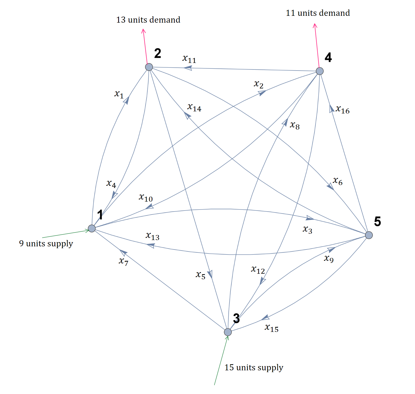
Figure 1: Network under consideration

6 Numerical example

In this section, we present an illustrative numerical example of our methodology in a transportation setup. We have used Wolfram Mathematica 10 for numerical computation.

Problem setup.

 Consider the following directed network with 5 nodes and 16 arcs as shown in Figure 1. Nodes 2 and 4 represent two retail centers with demands for 13 and 11 units of a certain product. The warehouses are denoted by nodes 1 and 3, which supply 9 and 15 units, respectively. Node 5 is a trans-shipment node. Different modes of shipment from one node to other is represented by the arcs in the figure, and these shipments are carried out by different organizations (carriers). The cost of a certain shipment depends on the number of products shipped; it is nonlinear and not necessarily convex. With each arc, we associate one carrier (player).

The cost functions for the players are listed in Table 1. The cost functions associated with players 5, 7, 10, and 15 are convex, and the cost functions associated with the rest of the players are nonconvex. Each of the players is trying to minimize its cost. The number of products carried by each player has to be non-negative, and the capacity of each player is represented by

$$u=(10,7,11,13,16,12,4,5,6,14,13,15,5,6,6,10),$$

where $u_{i}$ represents the maximum capacity for the number of products carried by player $i$.

Player	Cost function
1	$-\frac{x_{1}^{4}}{30}-\frac{13x_{1}^{3}}{15}+\frac{259x_{1}^{2}}{30}-\frac{263x_{1}}{15}+1$
2	$\frac{77x_{2}^{5}}{120}-\frac{247x_{2}^{4}}{24}+\frac{471x_{2}^{3}}{8}-\frac{3365x_{2}^{2}}{24}+\frac{6779x_{2}}{60}+1$
3	$\frac{47x_{3}^{4}}{24}-\frac{133x_{3}^{3}}{4}+\frac{4897x_{3}^{2}}{24}-\frac{2123x_{3}}{4}+485$
4	$\frac{323x_{4}^{5}}{3360}-\frac{2179x_{4}^{4}}{1120}+\frac{47393x_{4}^{3}}{3360}-\frac{48709x_{4}^{2}}{1120}+\frac{7885x_{4}}{168}+5$
5	$(x_{5}-1)^{2}$
6	$-\frac{x_{6}^{4}}{8}+\frac{25x_{6}^{3}}{12}-\frac{71x_{6}^{2}}{8}+\frac{95x_{6}}{12}+10$
7	$|x_{7}-5|$
8	$\frac{11x_{8}^{7}}{1260}-\frac{7x_{8}^{6}}{36}+\frac{119x_{8}^{5}}{72}-\frac{479x_{8}^{4}}{72}+\frac{4609x_{8}^{3}}{360}-\frac{803x_{8}^{2}}{72}+\frac{155x_{8}}{28}+1$
9	$-\frac{15}{16}x_{9}^{3}+\frac{365x_{9}^{2}}{16}-\frac{2865x_{9}}{16}+\frac{7315}{16}$
10	$(x_{10}-10)^{2}$
11	$\frac{5x_{11}^{4}}{6}-\frac{35x_{11}^{3}}{3}+\frac{355x_{11}^{2}}{6}-\frac{370x_{11}}{3}+90$
12	$\frac{5x_{12}^{4}}{6}-\frac{25x_{12}^{3}}{3}+\frac{175x_{12}^{2}}{6}-\frac{110x_{12}}{3}+15$
13	$\frac{5x_{13}^{4}}{6}-15x_{13}^{3}+\frac{595x_{13}^{2}}{6}-280x_{13}+285$
14	$\frac{5x_{14}^{4}}{6}-\frac{85x_{14}^{3}}{3}+\frac{2155x_{14}^{2}}{6}-\frac{6020x_{14}}{3}+4165$
15	$|x_{15}-7|$
16	$\begin{cases}x_{16}+1,&\text{if }0\leq x_{16}\leq 3\\ 0,&\textrm{if }4\leq x_{16}\leq 6\\ (x_{16}+1)^{3},&\textrm{if }7\leq x_{16}\leq 9\\ -\frac{x_{16}^{3}}{6}+\frac{13x_{16}^{2}}{2}-\frac{244x_{16}}{3}+330,&\textrm{else}\end{cases}$

Table 1: Cost functions for the players in the network considered

We seek efficient Pareto optimal points in this setup.

Computing node-arc incidence matrix and resource vector.

 First, we compute the node-arc incidence matrix associated with the network under consideration by following the procedure mentioned in the description of the mass balance constraint in Section 2. The resultant augmented node-arc incidence matrix of the network is:

$$\tilde{A}=\setcounter{MaxMatrixCols}{16}\begin{pmatrix}-1&-1&-1&1&0&0&1&0&0&1&0&0&1&0&0&0\\ 1&0&0&-1&-1&-1&0&0&0&0&1&0&0&1&0&0\\ 0&0&0&0&1&0&-1&-1&-1&0&0&1&0&0&1&0\\ 0&1&0&0&0&0&0&1&0&-1&-1&-1&0&0&0&1\\ 0&0&1&0&0&1&0&0&1&0&0&0&-1&-1&-1&-1\\ \end{pmatrix}$$

The vector $\tilde{b}$, where $\tilde{b}_{i}$ represents the demand or supply at node $i$, can be computed by recording the given demand or supply at each node and is given by $\tilde{b}=(9,-13,15,-11,0)$. As discussed in the description of the mass balance constraint in Section 2, we compute the full row rank node-arc incidence matrix $A$ by removing the 5th row of $\tilde{A}$ and the resource vector $b$ by removing the last component of $\tilde{b}$, i.e., $b=(9,-13,15,-11)$. So $A$ has 4 rows and 16 columns, and it is:

$$A=\setcounter{MaxMatrixCols}{16}\begin{pmatrix}-1&-1&-1&1&0&0&1&0&0&1&0&0&1&0&0&0\\ 1&0&0&-1&-1&-1&0&0&0&0&1&0&0&1&0&0\\ 0&0&0&0&1&0&-1&-1&-1&0&0&1&0&0&1&0\\ 0&1&0&0&0&0&0&1&0&-1&-1&-1&0&0&0&1\\ \end{pmatrix},$$

where we associate player $i$ with the $i$th column of $A$.

Reindexing the variables.

 To obtain the notational advantage as discussed in the comment after Lemma 1, we next rearrange the columns of the matrix $A$ so that the unimodular basis matrix comprising of the last 4 columns of $A$ constitutes the first $4$ columns in the new $A$ i.e., if $A=[A_{1}\mid A_{2}\mid\ldots\mid A_{4}\mid A_{5}\mid\ldots\mid A_{16}]$ then $\det([A_{1}\mid A_{2}\mid\ldots\mid A_{4}])=\pm 1$. We reindex the variables as follows. The last 4 players are reindexed as the first four players, and players 1 to 12 are reindexed as players 5 to 16. Due to this reindexing procedure, we need to reindex the upper bound vector $u$, where the last 4 indices become the first 4 indices, and the indices 1 to 12 become indices 5 to 16, i.e.,

$$u=(5,6,6,10,10,7,11,13,16,12,4,5,6,14,13,15).$$

Note that indices of $b$ would not change due to the reindexing procedure. We perform our computation on these reindexed variables and then revert the resultant efficient Pareto optimal solutions to the original indexing.

Problem transformation.

  Now we are in a position to transform the problem by following the methodology described in Section 3. First, we decouple the optimization problems for the last 12 players. In order to achieve that, we follow the constructive proofs of Lemma 4 and Theorem 3.1 to arrive at the following representation of the variable $x$ in terms of the new variable $z$:

$$x=\left(\begin{array}[]{c}x_{1}\\ x_{2}\\ x_{3}\\ x_{4}\\ x_{5}\\ x_{6}\\ x_{7}\\ x_{8}\\ x_{9}\\ x_{10}\\ x_{11}\\ x_{12}\\ x_{13}\\ x_{14}\\ x_{15}\\ x_{16}\end{array}\right)=\left(\begin{array}[]{c}z_{1}+z_{2}+z_{3}-z_{4}-z_{7}-z_{10}+9\\ -z_{1}+z_{4}+z_{5}+z_{6}-z_{11}-13\\ -z_{5}+z_{7}+z_{8}+z_{9}-z_{12}+15\\ -z_{2}-z_{8}+z_{10}+z_{11}+z_{12}-11\\ z_{1}\\ z_{2}\\ z_{3}\\ z_{4}\\ z_{5}\\ z_{6}\\ z_{7}\\ z_{8}\\ z_{9}\\ z_{10}\\ z_{11}\\ z_{12}\end{array}\right),$$ (25)

where the advantage of this transformation is that, for players 5 to 16, we have decoupled univariate optimization problems of the form (9) in $z$, and by solving these decoupled problems, we can reduce the constraint set significantly.

Solving the decoupled optimization problems.

 Next we solve the aforementioned decoupled univariate optimization problems for the last 12 players by following the procedure described in the last paragraph of Subsection 3.1. The solution set is given by Table 2; in this table, the sets of optimal solutions for players $5,6,\ldots,16$ are given by $D_{1},D_{2},\ldots,D_{12}$, respectively. Solving these 12 decoupled optimization problems immediately reduces the constraint set into a much smaller set, which we define as $D=\bigtimes_{i=1}^{12}D_{i}$.

$D_{1}$	$\{1\}$
$D_{2}$	$\{3\}$
$D_{3}$	$\{5\}$
$D_{4}$	$\{4,6\}$
$D_{5}$	$\{7,11\}$
$D_{6}$	$\{10\}$
$D_{7}$	$\{2\}$
$D_{8}$	{1}
$D_{9}$	$\{3\}$
$D_{10}$	$\{7\}$
$D_{11}$	$\{7\}$
$D_{12}$	$\{4,5,6,10,11\}$

Table 2: $D$ for the network under consideration

Elements	$z_{1}$	$z_{2}$	$z_{3}$	$z_{4}$	$z_{5}$	$z_{6}$	$z_{7}$	$z_{8}$	$z_{9}$	$z_{10}$	$z_{11}$	$z_{12}$
1	1	3	5	4	11	10	2	1	3	7	7	4
2	1	3	5	4	11	10	2	1	3	7	7	5
3	1	3	5	4	11	10	2	1	3	7	7	6
4	1	3	5	6	11	10	2	1	3	7	7	4
5	1	3	5	6	11	10	2	1	3	7	7	5
6	1	3	5	6	11	10	2	1	3	7	7	6

Table 3: Table listing elements of $\mathcal{F}$

Consensus reformulation for the first 4 players.

  Now we are in a position to transform the optimization problems for the first 4 players using (8) and consensus constraints as described in Subsection 3.2. By following the straightforward procedure of Subsection 3.2, we arrive at 4 optimization problems of the form (14), where each of the players 1 to 4 is optimizing its cost function over a common constraint set denoted by $\mathcal{F}$. Next we compute the points in $\mathcal{F}$.

Computing the points in $\mathcal{F}.$

  To compute the points in $\mathcal{F}$, we follow the methodology described in Subsection 4.2. Finding the points in $\mathcal{F}$ requires computing the reduced Groebner basis with respect to lexicographic ordering, denoted by $G_{\textrm{reduced},\succ_{\textrm{lex}}}$. We compute $G_{\textrm{reduced},\succ_{\textrm{lex}}}$ using the GroebnerBasis function in Wolfram Mathematica 10, and we find it to be not equal to $\{1\}$. Hence $\mathcal{F}$ is nonempty due to Lemma 5. Next we compute the points in $\mathcal{F}$ by following Algorithm 1; the list of computed points is given by Table 3.

Computing the efficient Pareto optimal points.

 The final step is computing the efficient Pareto optimal points from $\mathcal{F}$ by executing the three steps described in Algorithm 2. After applying Algorithm 2, we arrive at two efficient Pareto optimal points in variable $z$ as follows:

$$(1,3,5,4,11,10,2,1,3,7,7,5),$$

and

$$(1,3,5,6,11,10,2,1,3,7,7,6).$$

Using the relationship between $x$ and $z$ in (25), we can express these efficient Pareto optimal points in variable $x$ as follows:

$$(5,4,5,4,1,3,5,4,11,10,2,1,3,7,7,5),$$

and

$$(3,6,4,5,1,3,5,6,11,10,2,1,3,7,7,6).$$

Note that these efficient Pareto optimal points above are associated with the reindexed $x$. By reversing this reindexing, where indices 5 to 16 will be indices 1 to 12, and indices 1 to 4 will be indices 13 to 16, we arrive at the efficient Pareto optimal points in our original variable $x$ as follows:

$$(1,3,5,4,11,10,2,1,3,7,7,5,5,4,5,4),$$

and

$$(1,3,5,6,11,10,2,1,3,7,7,6,3,6,4,5).$$

7 Conclusions

In this paper, we have proposed a multi-player extension of the minimum cost flow problem inspired by a multi-player transportation problem. We have associated one player with each arc of a directed connected network, each trying to minimize its cost subject to the network flow constraints. The cost can be any general nonlinear function, and the flow through each arc is integer-valued. In this multi-player setup, we have presented algorithms to compute an efficient Pareto optimal point, which is a good compromise solution between the utopian vector optimality and the generic Pareto optimality and is a Nash equilibrium if our problem is transformed into an $n$-person finite static game in normal form.

Some concluding remarks on the limitations of our methodology are as follows. First, at the heart of our methodology is the transformation provided by Theorem 3.1, which decouples the optimization problems for the last $n-m$ players. Each of these decoupled optimization problems is univariate over a discrete interval and is easy to solve. This can potentially allow us to work in a much smaller search space. So if we have a system where $n-m>m\Leftrightarrow m<\frac{n}{2}$, then it will be convenient from a numerical point of view. Second, computation of Pareto optimal points depends on determining the points in $\mathcal{F}$ using Groebner basis. Calculating Groebner basis can be numerically challenging for large system (Cox et al., 2007, pages 111-112), though significant speed-up has been achieved in recent years by computer algebra packages such as Macaulry2, SINGULAR, FGb, and Mathematica.

Appendix

Proof of Lemma 1

Any basic solution of $\mathop{\bf relaxed}P$ can be constructed as follows. Take $m$ linearly independent columns

$$A_{B(1)},A_{B(2)},\ldots,A_{B(m)},$$

where $B(1),B(2),\ldots,B(m)$ are the indices of those columns. Construct the basis matrix

$$B=\begin{bmatrix}A_{B(1)}&&A_{B(2)}&&\cdots&&A_{B(m)}\end{bmatrix}.$$

Set $x_{B}=(x_{B(1)},x_{B(2)},\ldots,x_{B(m)})=B^{-1}b$, which is called the basic variable in linear programming theory. Set the rest of the components of $x$ (called the nonbasic variable) to be zero, i.e.,

$$x_{NB}=(x_{NB(1)},x_{NB(2)},\ldots,x_{NB(n-m)})=(0,0,\ldots,0).$$

The resultant $x$ will be a basic solution of $\mathop{\bf relaxed}P$ [Bertsimas and Tsitsiklis, 1997, Theorem 2.4].

Suppose there is an integer basic solution in $\mathop{\bf relaxed}P$. Denote that integer basic solution by $\bar{x}$ and the associated basis matrix by $\bar{B}$. The nonbasic variables are integers (zeros) in every basic solution, so the basic variables $\bar{x}_{\bar{B}}=\bar{B}^{-1}b$ has to be an integer vector for any integer $b$. Now from Cramer’s rule [Bertsimas and Weismantel, 2005, Proposition 3.1],

$$\left(\forall b\in\mathbf{Z}^{m}\right)\quad\left(\bar{x}_{\bar{B}}=\bar{B}^{-1}b\in\mathbf{Z}^{m}\Leftrightarrow\forall i\in[m]\quad\bar{x}_{\bar{B}(i)}=\frac{\det\bar{B}^{i}}{\det\bar{B}}\in\mathbf{Z}\right),$$

where $\bar{B}^{i}$ is the same as $\bar{B}$, except the $i$th column has been replaced with $\bar{b}$. Now $\det\bar{B}^{i}\in\mathbf{Z}$ because $b$ is an integer vector. So having integer basic solution is equivalent to $\det\bar{B}=\pm 1$, i.e., $\bar{B}$ is unimodular. $\blacksquare$

Proof of Lemma 2

First, note that unimodularity of $B$ is equivalent to unimodularity of $B^{-1}$, which we show easily as follows. First note that, $\det\left(B^{-1}\right)=\frac{1}{\det B}=\frac{1}{\pm 1}=\pm 1$. Each component of $B^{-1}$ is a subdeterminant of $B$ divided by $\det B$. As $B\in\mathbf{Z}^{m\times m}$ and $\det B=\pm 1$, each component of $B^{-1}$ is an integer. Thus $B^{-1}$ is a unimodular matrix. Similarly, unimodularity of $B^{-1}$ implies $B$ is unimodular.

So $C=B^{-1}A\in\mathbf{Z}^{m\times n}$ and $d=B^{-1}b\in\mathbf{Z}^{m}$ as $A$ and $b$ are integer matrices. As multiplying both sides of a linear system by an invertible matrix does not change the solution, we have $Ax=b\Leftrightarrow B^{-1}Ax=B^{-1}b\Leftrightarrow Cx=d$. Thus we arrive at the claim. $\blacksquare$

Proof of Lemma 3

First, recall that the following operations on a matrix are called elementary integer column operations: (i) adding an integer multiple of one column to another column, (ii) exchanging two columns, and (iii) multiplying a column by -1.

The matrix $C$ is of the form:

$$C = B^{-1}A$$

$$= B^{-1}\left[B\mid A_{m+1}\mid A_{m+2}\mid\cdots\mid A_{n}\right]$$

$$= \begin{bmatrix}1&0&\cdots&0&C_{1,m+1}&C_{1,m+2}&\cdots&C_{1,n}\\ 0&1&\cdots&0&C_{2,m+1}&C_{2,m+2}&\cdots&C_{2,n}\\ \vdots&\vdots&\vdots&\vdots&\vdots&\vdots&\vdots&\vdots\\ 0&0&\cdots&1&C_{m,m+1}&C_{m,m+2}&\cdots&C_{m,n}\end{bmatrix}$$

Consider the first column of $C$. For all $j=m+1,m+2,\ldots,n$, we multiply the first column of $C$, $C_{1}=e_{1}$ of $C$ by $-C_{1,j}$ and then add it to $C_{i}$. Thus $C$ is transformed to

$$\begin{bmatrix}1&0&\cdots&0&0&0&\cdots&0\\ 0&1&\cdots&0&C_{2,m+1}&C_{2,m+2}&\cdots&C_{2,n}\\ \vdots&\vdots&\vdots&\vdots&\vdots&\vdots&\vdots&\vdots\\ 0&0&\cdots&1&C_{m,m+1}&C_{m,m+2}&\cdots&C_{m,n}\end{bmatrix}$$

Similarly for column indices, $i=2,3,\ldots,m$, respectively we do the following. For $j=m+1,m+2,\cdots,n$, we multiply the $i$th column $e_{i}$ with $-C_{i,j}$ and add it to $C_{j}$. In the end, the Hermite normal form becomes:

$$\begin{bmatrix}1&0&\cdots&0&0&0&\cdots&0\\ 0&1&\cdots&0&0&0&\cdots&0\\ \vdots&\vdots&\vdots&\vdots&\vdots&\vdots&\vdots&\vdots\\ 0&0&\cdots&1&0&0&\cdots&0\end{bmatrix}.$$

The steps describing the process in Lemma 3 can be summarized by Algorithm 3, which we are going to use to prove Lemma 4. $\blacksquare$

Algorithm 3 Converting $C$ to $[I|0]$

1:procedure Converting $C$ to $[I|0]$

2:     for $i:=1,2,\ldots,m$ do

3:         for $j:=m+1,m+2,\ldots,n$ do

4:              $C_{j}:=C_{j}-C_{i,j}e_{i}$

5:         end for

6:     end for

7:end procedure

Proof of Lemma 4

If we multiply column $C_{i}$ of a matrix $C$ with an integer factor $\gamma$ and subsequently add it to another column $C_{j}$, then it is equivalent to right multiplying the matrix $C$ with a matrix $I+\gamma I_{ij}$ (recall that the matrix $I_{ij}$ has a one in $(i,j)$th position and zero everywhere else). Note that $I+\gamma I_{ij}$ is a triangular matrix with diagonal entries being one, $\gamma$ being on the $(i,j)$th position, and zero everywhere else. As the determinant of a triangular matrix is the product of its diagonal entries, $\det(I+\gamma I_{ij})=1$. So $I+\gamma I_{ij}$ is a unimodular matrix. Furthermore, step 4 of the procedure above to convert $C$ to Hermite normal form, i.e., $C_{j}=C_{j}-C_{i,j}e_{i}$ is equivalent to left multiplying the current matrix with $I-C_{i,j}I_{ij}$. So the inner loop of the procedure above over $j=m+1,m+2,\ldots,n$ (lines 2-4) can be achieved by left multiplying the current matrix with

$$U_{i}=\prod_{j=m+1}^{n}(I-C_{ij}I_{ij})=(I-C_{i,m+1}I_{i,m+1})(I-C_{i,m+2}I_{i,m+2})\cdots(I-C_{i,n}I_{i,n})$$

As each of the matrices in the product is a unimodular matrix and determinant of multiplication of square matrices of same size is equal to multiplication of determinant of those matrices, we have $\det(U_{i})=1$. So $U_{i}$ is a unimodular matrix. Structurally the $i$th row of $U_{i}$, denoted by $u_{i}^{T}$, has a $1$ on $i$th position, has $-C_{i,j}$ on $j$th position for $j=m+1,m+2,\ldots,n$, and zero everywhere else. Any other $k$th row $(k\neq i)$ of $U_{i}$ is $e_{k}^{T}$. So we can convert $C$ to its Hermite normal form by repeatedly left multiplying $C$ with $U_{1},U_{2},\ldots,U_{m}$, respectively. This is equivalent to left multiplying $C$ with one single matrix $U=\prod_{i=1}^{m}U_{i}$. The final matrix $U$ is unimodular as it is multiplication of unimodular matrices. $\blacksquare$

Proof of Theorem 1

Let $y=U^{-1}x$. As $U$ is unimodular, $U^{-1}$ is also unimodular. Hence $x\in\mathbf{Z}^{n}\Leftrightarrow y\in\mathbf{Z}^{n}$. Let $y=(y_{1},y_{2})$, where $y_{1}\in\mathbf{Z}^{m}$ and $y_{2}\in\mathbf{Z}^{n-m}$. Then

$$Q\neq\emptyset$$

$$\Leftrightarrow \exists x\in\mathbf{Z}^{n}\;\left(Cx=d\right)$$

$$\Leftrightarrow \exists y\in\mathbf{Z}^{n}\;\left(CUy=\begin{bmatrix}I&0\end{bmatrix}\begin{bmatrix}y_{1}\\ y_{2}\end{bmatrix}=y_{1}=d\right).$$

As $d=B^{-1}b\in\mathbf{Z}^{m}$ (Lemma 2), by taking $y=\begin{bmatrix}y_{1}\\ y_{2}\end{bmatrix}=\begin{bmatrix}B^{-1}b\\ z\end{bmatrix}\in\mathbf{Z}^{n}$, where $z\in\mathbf{Z}^{n-m}$, we can satisfy the condition above. Thus $Q$ is nonempty.

Now for any $x$, we can maximally decompose it in terms of $z$ as:

$$x\in Q\Leftrightarrow x=Uy =\begin{bmatrix}I_{m}&-B^{-1}A_{[1:m,m+1:n]}\\ 0_{n-m\times m}&I_{n-m}.\end{bmatrix}\begin{bmatrix}B^{-1}b\\ z\end{bmatrix}$$

$$=\begin{bmatrix}B^{-1}\left(b-A_{[1:m,m+1:n]}z\right)\\ z\end{bmatrix}$$

$$=\begin{bmatrix}d_{1}-h_{1}^{T}z\\ d_{2}-h_{2}^{T}z\\ \vdots\\ d_{m}-h_{m}^{T}z\\ z_{1}\\ \vdots\\ z_{n-m}\end{bmatrix},$$

where the last $n-m$ variables are completely decoupled in terms of $z$. Note that the decomposition is maximal by construction and cannot be extended any further in general cases. $\blacksquare$

Proof of Theorem 3

The proof sketch is as follows. The elements of $\mathcal{F}$ are the solution of the polynomial system:

$$\left(\forall i\in[m]\right)\quad q_{i}(z)=0$$

$$\left(\forall j\in[n-m]\right)\quad r_{j}(z)=0.$$ (26)

We prove in two steps. In step $1$, we show that the polynomial system (26) is feasible if and only if

$$1\notin\mathbf{ideal}\left\{q_{1},\ldots,q_{m},r_{1},\ldots,r_{n-m}\right\}.$$

Then in step $2$, we show that, $1\notin\mathbf{ideal}\left\{q_{1},\ldots,q_{m},r_{1},\ldots,r_{n-m}\right\}$ is equivalent to $G_{\textrm{reduced},\succ}\neq\{1\}$.

Step 1. Polynomial system (26) is feasible if and only if $1\notin\mathbf{ideal}\left\{q_{1},\ldots,q_{m},r_{1},\ldots,r_{n-m}\right\}.$

We prove necessity first and then sufficiency.
($\Rightarrow$)

Assume system (26) is feasible, but $1\in\mathbf{ideal}\left\{q_{1},\ldots,q_{m},r_{1},\ldots,r_{n-m}\right\}$. That means

$$\left(\exists h_{1},\ldots,h_{m},s_{1},\ldots,s_{n-m}\in\mathbf{C}[z]\right)\left(\forall z\in\mathbf{C}^{n-m}\right)\quad 1=\sum_{i=1}^{m}h_{i}(z)q_{i}(z)+\sum_{i=1}^{n-m}s_{i}(z)r_{i}(z),$$ (27)

and

$$\left(\exists\bar{z}\in\mathbf{Z}{}^{n-m}\right)\bigg{(} \left(\forall i\in[m]\right)\quad q_{i}(\bar{z})=0,$$

$$\left(\forall i\in[n-m]\right)\quad r_{i}(\bar{z})=0\bigg{)}.$$ (28)

Putting $z=\bar{z}$ in (27) and using (28) we get $1=0$, so we have a contradiction.
($\Leftarrow$)

We want to show that if $1\not\in\mathbf{ideal}\{q_{1},\cdots,q_{m},r_{1},\cdots,r_{n-m}\}$, then the polynomial system (26) is feasible. We prove the contrapositive again: if the polynomial system (26) is infeasible in integers, then $1\in\mathbf{ideal}\{q_{1},\cdots,q_{m},r_{1},\cdots,r_{n-m}\}$.

First, we show that, feasibility of the system in $\mathbf{C}^{n-m}$ is equivalent to feasibility in $\mathbf{Z}^{n-m}$. As $\mathbf{Z}^{n-m}\subset\mathbf{C}^{n-m}$, if the polynomial system is infeasible in $\mathbf{C}^{n-m}$, it is infeasible in $\mathbf{Z}^{n-m}$. Also, if the polynomial system is infeasible in $\mathbf{Z}^{n-m}$, then it will be infeasible in $\mathbf{C}^{n-m}$. We show this by contradiction. Assume the system system is infeasible in $\mathbf{Z}^{n-m}$ but feasible in $\mathbf{C}^{n-m}$ i.e., $\mathbf{C}^{n-m}\setminus\mathbf{Z}^{n-m}$. Let that feasible solution be $\tilde{z}\in\mathbf{C}^{n-m}\setminus\mathbf{Z}^{n-m}$, so there is at least one component of it (say $\tilde{i}$) such that $\tilde{z}_{\tilde{i}}\in\mathbf{C}\setminus\mathbf{Z}$. Now

$$r_{\tilde{i}}(\tilde{z})=(\tilde{z}_{\tilde{i}}-z_{i,1})(\tilde{z}_{\tilde{i}}-z_{i,2})\ldots(\tilde{z}_{\tilde{i}}-z_{i,p_{i}}),$$

where, by construction, each of the elements of the set $D_{i}=\left\{z_{i,1},z_{i,2},\ldots,z_{i,p_{i}}\right\}$ are integers and different from each other, so each component in the product $r_{\tilde{i}}(\tilde{z})$ are nonzero complex numbers with the absence of complex conjugates. So $r_{\tilde{i}}(\tilde{z})\neq 0$, which is a contradiction.

If the polynomial system is infeasible in $\mathbf{C}^{n-m}$, then it is equivalent to saying that,

$$V(q_{1},\ldots,q_{m},r_{1},\ldots,r_{n-m})=\emptyset,$$

where $V$ has been defined in (15). Then using the Weak Nullstellensatz, we have

$$\mathbf{ideal}\{q_{1},\ldots,q_{m},r_{1},\ldots,r_{n-m}\}=\mathbf{C}[z_{1},z_{2},\ldots,z_{n-m}].$$

As $1\in\mathbf{C}[z_{1},z_{2},\ldots,z_{n-m}]$, this means $1\in\mathbf{ideal}\{q_{1},\ldots,q_{m},r_{1},\ldots,r_{n-m}\}$.

Step 2. Now we show $1\notin\mathbf{ideal}\left\{q_{1},\ldots,q_{m},r_{1},\ldots,r_{n-m}\right\}$ is equivalent to $G_{\textrm{reduced},\succ}\neq\{1\}.$

We have shown that feasibility of the system in $\mathbf{C}^{n-m}$ is equivalent to feasibility in $\mathbf{Z}^{n-m}$. As a result, we can work over complex numbers, which is a algebraically closed field. This allows us to apply consistency algorithm [Cox et al., 2007, page 172], which states that $1\notin\mathbf{ideal}\left\{q_{1},\ldots,q_{m},r_{1},\ldots,r_{n-m}\right\}$ if and only if $G_{\textrm{reduced},\succ}\neq\{1\}$ . $\blacksquare$

Proof of Lemma 5

By Theorem 4.2, we have $\mathcal{F}\neq\emptyset$. So from the definition of affine variety in (15) and (13) we can write $\mathcal{F}$ as:

$$\mathcal{F}=V\left(q_{1},\ldots,q_{m},r_{1},\ldots,r_{n-m}\right)\cap\mathbf{Z}^{n-m}.$$

From the equation above and (16) we have,

$$\mathcal{F} = V\left(q_{1},\ldots,q_{m},r_{1},\ldots,r_{n-m}\right)$$

$$\neq \emptyset.$$

By definition of basis, we have $\mathbf{ideal}\left\{q_{1},\ldots,q_{m},r_{1},\ldots,r_{n-m}\right\}=\mathbf{ideal}\left\{G_{\textrm{reduced},\succ_{\textrm{lex}}}\right\}$, which implies

$$V\left(q_{1},\ldots,q_{m},r_{1},\ldots,r_{n-m}\right)=V\left(G_{\textrm{reduced},\succ_{\textrm{lex}}}\right)$$

due to [Proposition 2, Cox et al., 2007, page 32]. So $\mathcal{F}=V\left(G_{\textrm{reduced},\succ_{\textrm{lex}}}\right).$ $\blacksquare$

Proof of Lemma 6

Using Theorem 4.2, we have $G_{\textrm{reduced},\succ_{\textrm{lex}}}\neq\emptyset$. So by the elimination theorem [Theorem 2, Cox et al., 2007, page 116] $V\left(G_{n-m-1}\right)$ is nonempty and will contain the list of all possible $z_{n-m}$ coordinates for the points in $\mathcal{F}$. As $G_{\textrm{reduced},\succ_{\textrm{lex}}}\neq\emptyset$, when moving from one step to the next, not all the affine varieties associated with the univariate polynomials (after replacing the previous coordinates into the elimination ideal) can be empty due to the extension theorem [Theorem 3, Cox et al., 2007, page 118]. Using this logic repeatedly, the final step will give us $\mathcal{F}=V(G_{\textrm{reduced},\succ_{\textrm{lex}}})\neq\emptyset$. $\blacksquare$

Proof of Lemma 7

Follows from (19), (17) and (20). $\blacksquare$

Proof of Lemma 8

For any $i\in[m]$,

$$x_{s_{i}}\in X_{s_{i}}^{*}$$

$$\Leftrightarrow d_{s_{i}}-h_{s_{i}}^{T}z\in X_{s_{i}}^{*}$$

$$\Leftrightarrow z\in\mathcal{F}_{s_{i}}^{*},$$

where the second line follows from (8). So

$$\left(\begin{aligned} &\mathrm{minimize}_{x_{s_{i}}}&&f_{s_{i}}(x_{s_{i}})\\ &\mathrm{subject\;to}&&x_{s_{i}}\in X_{s_{i}}\end{aligned}\right)$$

$$= \left(\begin{aligned} &\mathrm{minimize}_{x_{s_{i}}}&&f_{s_{i}}(d_{s_{i}}-h_{s_{i}}^{T}z)\\ &\mathrm{subject\;to}&&z\in\mathcal{F}_{s_{i-1}}^{*}\end{aligned}\right),$$

where the second line follows from (20) in Algorithm 2. $\blacksquare$

Proof of Lemma 9

As $\mathcal{F}\neq\emptyset$, $X_{s_{1}}:=\left\{d_{s_{1}}-h_{s_{1}}^{T}z^{(s_{1})}\mid z^{(s_{1})}\in\mathcal{F}\right\}\neq\emptyset$. Assume, for $i\in[m]$, we have $\mathcal{F}_{s_{i}}^{*}\neq\emptyset$. Then $X_{s_{i+1}}:=\left\{d_{s_{i+1}}-h_{s_{i+1}}^{T}z\mid z\in\mbox{$\mathcal{F}$}_{s_{i}}^{*}\right\}=d_{s_{i+1}}-h_{s_{i+1}}^{T}\mathcal{F}_{s_{i}}^{*}\neq\emptyset$. The subsequent optimization problem is

$$\mathrm{minimize}_{x_{s_{i+1}}} f_{s_{i+1}}(x_{s_{i+1}})$$

$$\mathrm{subject\;to} x_{s_{i+1}}\in X_{s_{i+1}}.$$

As we are optimizing over a finite and countable set, a minimizer will exist. So $X_{s_{i+1}}^{*}\neq\emptyset$. Hence $\mathcal{F}_{s_{i}}^{*}=\bigcup_{x_{i}\in X_{s_{i}}^{*}}(X_{s_{i}}^{*})^{-1}(x_{i})\neq\emptyset$. So for any $i=1,\ldots,m$, we have $\mathcal{F}_{s_{i}}^{*}$ nonempty. $\blacksquare$

Proof of Theorem 4

We want to show that $x^{*}$ is feasible, and for every $x\in P,i\in[n]$ , if we have $f_{i}(x_{i}^{*})\geq f_{i}(x_{i})$, then for every $j\in[n]$, $f_{j}(x_{j}^{*})=f_{j}(x_{j})$. Using (21) and (8), we can translate the Pareto optimality condition in $z$ as follows. Consider a $z\in\mathbf{Z}^{n-m}$ such that

$$(0,\ldots,0)\preceq\left(\left(d_{i}-h_{i}^{T}z\right)_{i=1}^{m}\right),z)\preceq (u_{1},\ldots,u_{n}),$$ (29)

and suppose

$$\left(\left(f_{i}(d_{i}-h_{i}^{T}z^{*})_{i=1}^{m}\right),\left(f_{m+i}(z_{i}^{*})\right)_{i=1}^{n-m}\right)\succeq \left(\left(f_{i}(d_{i}-h_{i}^{T}z)_{i=1}^{m}\right),\left(f_{m+i}(z_{i})\right)_{i=1}^{n-m}\right).$$ (30)

Then we want to show that:

$$\left(\left(f_{i}(d_{i}-h_{i}^{T}z^{*})_{i=1}^{m}\right),\left(f_{m+i}(z_{i}^{*})\right)_{i=1}^{n-m}\right)= \left(\left(f_{i}(d_{i}-h_{i}^{T}z)_{i=1}^{m}\right),\left(f_{m+i}(z_{i})\right)_{i=1}^{n-m}\right)$$ (31)

Let us start with the last $n-m$ rows. As, $z^{*}\in\mathcal{F}_{s_{m}}^{*}\subseteq\mathcal{F}\subseteq D$ and by construction, $D=\bigtimes_{i=1}^{n-m}D_{i}$, where any element of $D_{i}$ is a minimizer of (9), so

$$\left(f_{m+i}(z_{i}^{*})\right)_{i=1}^{n-m}\succeq\left(f_{m+i}(z_{i})\right)_{i=1}^{n-m}$$

implies

$$\left(f_{m+i}(z_{i}^{*})\right)_{i=1}^{n-m}=\left(f_{m+i}(z_{i})\right)_{i=1}^{n-m}.$$

In the subsequent steps, it suffices to confine $z\in D$, as otherwise last $n-m$ inequalities of (30) will be violated. Now let us consider the first $m$ inequalities of (30) As discussed in Section 3.2, any $z$ is in $D$ which obeys the inequalities $0\leq d_{i}-h_{i}^{T}z\leq u_{i}$ for $i=1,\ldots,m$; this is equivalent to $z\in\mathcal{F}\subseteq D$. Consider, $s_{1}\in[m]$ . Lemmas 7 and 8 implies that $z^{*}$ solves the following optimization problem $\min_{z}\{f_{s_{1}}(d_{s_{1}}-h_{s_{1}}^{T}z)\mid z\in\mathcal{F}\}=\min_{x_{s_{1}}}\{f_{s_{1}}(x_{s_{1}})\mid x_{s_{1}}\in X_{s_{1}}\}$, which has solution $x_{s_{1}}^{*}\in X_{s_{1}}^{*}\Leftrightarrow z^{*}\in\mathcal{F}_{s_{1}}^{*}\supseteq\mathcal{F}_{s_{m}}^{*}$. So $f_{s_{1}}(d_{s_{1}}-h_{s_{1}}^{T}z)\leq f_{s_{1}}(d_{s_{1}}-h_{s_{1}}^{T}z^{*})$ implies $f_{s_{1}}(d_{s_{1}}-h_{s_{1}}^{T}z)=f_{s_{1}}(d_{s_{1}}-h_{s_{1}}^{T}z^{*})$ and $z\in\mathcal{F}_{s_{1}}^{*}$.

Consider $s_{2}\in[m]\setminus\{s_{1}\}$. First, note that $z\in\mathcal{F}_{s_{1}}^{*}$, otherwise $f_{s_{1}}(d_{s_{1}}-h_{s_{1}}^{T}z)\leq f_{s_{1}}(d_{s_{1}}-h_{s_{1}}^{T}z^{*})$ will not hold. Now the $x_{s_{2}}^{*}$ associated with $z^{*}$ solves the following optimization problem $\min_{x_{s_{2}}}\{f_{s_{2}}(x_{s_{2}})\mid x_{s_{2}}\in X_{s_{2}}\}=\min_{z}\{f_{s_{2}}(d_{s_{2}}-h_{s_{2}}^{T}z)\mid z\in\mathcal{F}_{s_{1}}^{*}\}$, where an optimal solution to the first line will be in $X_{s_{2}}^{*}$ and the optimal solution to the second line will be in $\mathcal{F}_{s_{2}}^{*}$ (Lemma 8). So combining $f_{s_{2}}(d_{s_{2}}-h_{s_{2}}^{T}z)\leq f_{s_{2}}(d_{s_{2}}-h_{s_{2}}^{T}z^{*})$ and $z\in\mathcal{F}_{s_{1}}^{*}$ implies $f_{s_{2}}(d_{s_{2}}-h_{s_{2}}^{T}z)=f_{s_{2}}(d_{s_{2}}-h_{s_{2}}^{T}z^{*}).$ Repeating a similar argument for $i=s_{3},s_{4},\ldots,s_{m}$, we can show that

$$\left(\forall i\in\{s_{1},\ldots,s_{m}\}\right)\quad f_{s_{2}}(d_{s_{2}}-h_{s_{2}}^{T}z)=f_{s_{i}}(d_{s_{i}}-h_{s_{i}}^{T}z^{*}).$$

Thus we have arrived at (31). $\blacksquare$

References

• Gupta and Pavel [2016] Shuvomoy Das Gupta and Lacra Pavel. Multi-player minimum cost flow problems with nonconvex costs and integer flows. In Decision and Control (CDC), 2016 IEEE 55th Conference on, pages 7617–7622. IEEE, 2016.
• Turban et al. [2017] Efraim Turban, Jon Outland, David King, Jae Kyu Lee, Ting-Peng Liang, and Deborrah C Turban. Electronic Commerce 2018: A Managerial and Social Networks Perspective. Springer, Berlin, 2017.
• Galloway [1998] Scott Galloway. The Four: The Hidden DNA of Amazon, Apple, Facebook, and Google. Portfolio, New York, 2017.
• Li [2014] Ling Li. Managing Supply Chain and Logistics: Competitive Strategy for a Sustainable Future. World Scientific Publishing Co Inc, 2014.
• Mendez et al. [2017] Victor M Mendez, Carlos A Monje Jr, and Vinn White. Beyond traffic: Trends and choices 2045: A national dialogue about future transportation opportunities and challenges. In Disrupting Mobility, pages 3–20. Springer, Cham, 2017.
• Laseter and Rabinovich [2011] Timothy M Laseter and Elliot Rabinovich. Internet retail operations: integrating theory and practice for managers. CRC Press, 2011.
• Boyd and Vandenberghe [2004] Stephen Boyd and Lieven Vandenberghe. Convex optimization. Cambridge university press, 2004.
• Miettinen [2012] Kaisa Miettinen. Nonlinear multiobjective optimization, volume 12. Springer Science & Business Media, 2012.
• Ahuja et al. [1993] Ravindra K Ahuja, Thomas L Magnanti, and James B Orlin. Network Flows: Theory, Algorithms, and Applications. Prentice Hall, 1993.
• Bertsimas et al. [2013] Dimitris Bertsimas, Ebrahim Nasrabadi, and Sebastian Stiller. Robust and adaptive network flows. Operations Research, 61(5):1218–1242, 2013.
• Vaidyanathan and Ahuja [2010] Balachandran Vaidyanathan and Ravindra K Ahuja. Fast algorithms for specially structured minimum cost flow problems with applications. Operations research, 58(6):1681–1696, 2010.
• Magnanti and Wong [1984] Thomas L Magnanti and Richard T Wong. Network design and transportation planning: Models and algorithms. Transportation science, 18(1):1–55, 1984.
• Graves and Orlin [1985] Stephen C Graves and James B Orlin. A minimum concave-cost dynamic network flow problem with an application to lot-sizing. Networks, 15(1):59–71, 1985.
• Daskin [2011] Mark S Daskin. Network and discrete location: models, algorithms, and applications. John Wiley & Sons, 2011.
• Feltenmark and Lindberg [1997] Stefan Feltenmark and Per Olof Lindberg. Network methods for head-dependent hydro power scheduling. Springer, 1997.
• Yaged [1971] Bt Yaged. Minimum cost routing for static network models. Networks, 1(2):139–172, 1971.
• He et al. [2015] Qie He, Shabbir Ahmed, and George L Nemhauser. Minimum concave cost flow over a grid network. Mathematical Programming, 150(1):79–98, 2015.
• Tuy et al. [1995] Hoang Tuy, Saied Ghannadan, Athanasios Migdalas, and Peter Värbrand. The minimum concave cost network flow problem with fixed numbers of sources and nonlinear arc costs. Journal of Global Optimization, 6(2):135–151, 1995.
• Fontes et al. [2006] Dalila BMM Fontes, Eleni Hadjiconstantinou, and Nicos Christofides. A branch-and-bound algorithm for concave network flow problems. Journal of Global Optimization, 34(1):127–155, 2006.
• Zangwill [1968] Willard I Zangwill. Minimum concave cost flows in certain networks. Management Science, 14(7):429–450, 1968.
• Jorjani and Lamar [1994] S Jorjani and BW Lamar. Cash flow management network models with quantity discounting. Omega, 22(2):149–155, 1994.
• Gamarnik et al. [2012] David Gamarnik, Devavrat Shah, and Yehua Wei. Belief propagation for min-cost network flow: Convergence and correctness. Operations research, 60(2):410–428, 2012.
• Kim and Pardalos [2000] Dukwon Kim and Panos M Pardalos. A dynamic domain contraction algorithm for nonconvex piecewise linear network flow problems. Journal of Global optimization, 17(1-4):225–234, 2000.
• Yan et al. [2011] Shangyao Yan, Yu-Lin Shih, and Wang-Tsang Lee. A particle swarm optimization-based hybrid algorithm for minimum concave cost network flow problems. Journal of Global Optimization, 49(4):539–559, 2011.
• Raith and Ehrgott [2009] Andrea Raith and Matthias Ehrgott. A two-phase algorithm for the biobjective integer minimum cost flow problem. Computers & Operations Research, 36(6):1945–1954, 2009.
• Lee and Pulat [1993] Haijune Lee and P Simin Pulat. Bicriteria network flow problems: Integer case. European Journal of Operational Research, 66(1):148–157, 1993.
• Eusébio and Figueira [2009] Augusto Eusébio and José Rui Figueira. Finding non-dominated solutions in bi-objective integer network flow problems. Computers & Operations Research, 36(9):2554–2564, 2009.
• Hernández et al. [2011] Salvador Hernández, Srinivas Peeta, and George Kalafatas. A less-than-truckload carrier collaboration planning problem under dynamic capacities. Transportation Research Part E: Logistics and Transportation Review, 47(6):933–946, 2011.
• Barnhart et al. [1996] Cynthia Barnhart, Christopher A Hane, and Pamela H Vance. Integer multicommodity flow problems. In Integer Programming and Combinatorial Optimization, pages 58–71. Springer, Berlin, 1996.
• Brunetta et al. [2000] Lorenzo Brunetta, Michele Conforti, and Matteo Fischetti. A polyhedral approach to an integer multicommodity flow problem. Discrete Applied Mathematics, 101(1):13–36, 2000.
• Ozdaglar and Bertsekas [2004] Asuman E Ozdaglar and Dimitri P Bertsekas. Optimal solution of integer multicommodity flow problems with application in optical networks. In Frontiers in global optimization, pages 411–435. Springer, Boston, 2004.
• Bertsimas and Tsitsiklis [1997] Dimitris Bertsimas and John N Tsitsiklis. Introduction to linear optimization, volume 6. Athena Scientific Belmont, MA, 1997.
• Basar and Olsder [1995] Tamer Basar and Geert Jan Olsder. Dynamic noncooperative game theory, volume 23. SIAM, 1995.
• Schrijver [1998] Alexander Schrijver. Theory of linear and integer programming. John Wiley & Sons, 1998.
• Bertsimas and Weismantel [2005] Dimitris Bertsimas and Robert Weismantel. Optimization over integers, volume 13. Dynamic Ideas Belmont, 2005.
• Parikh and Boyd [2013] Neal Parikh and Stephen Boyd. Proximal algorithms. Foundations and Trends in optimization, 1(3):123–231, 2013.
• Cox et al. [2007] David Cox, John Little, and Donal O’shea. Ideals, varieties, and algorithms, volume 3. Springer, 2007.
• Bertsekas et al. [2003] Dimitri P. Bertsekas, Asuman E. Ozdaglar, and Angelia Nedic. Convex analysis and optimization. Athena scientific optimization and computation series. Athena Scientific, Belmont (Mass.), 2003. ISBN 1-886529-45-0.