Optimizing Sparse Matrix-Vector Multiplication on Emerging Many-Core Architectures

Abstract

Sparse matrix vector multiplication (SpMV) is one of the most common operations in scientific and high-performance applications, and is often responsible for the application performance bottleneck. While the sparse matrix representation has a significant impact on the resulting application performance, choosing the right representation typically relies on expert knowledge and trial and error. This paper provides the first comprehensive study on the impact of sparse matrix representations on two emerging many-core architectures: the Intel’s Knights Landing (KNL) XeonPhi and the ARM-based FT-2000Plus (FTP). Our large-scale experiments involved over 9,500 distinct profiling runs performed on 956 sparse datasets and five mainstream SpMV representations. We show that the best sparse matrix representation depends on the underlying architecture and the program input. To help developers to choose the optimal matrix representation, we employ machine learning to develop a predictive model. Our model is first trained offline using a set of training examples. The learned model can be used to predict the best matrix representation for any unseen input for a given architecture. We show that our model delivers on average 95% and 91% of the best available performance on KNL and FTP respectively, and it achieves this with no runtime profiling overhead.

I Introduction

Sparse matrix-vector multiplication (SpMV) is commonly seen in scientific and high-performance applications [33, 48]. It is often responsible for the performance bottleneck and notoriously difficult to optimize [22, 21, 2]. Achieving a good SpMV performance is challenging because its performance is heavily affected by the density of nonzero entries or their sparsity pattern. As the processor is getting increasingly diverse and complex, optimizing SpMV becomes harder.

Prior research has shown that the sparse matrix storage format (or representation) can have a significant impact on the resulting performance, and the optimal representation depends on the underlying architecture as well as the size and the content of the matrices [1, 19, 46, 4, 3]. While there is already an extensive body of study on optimizing SpMV on SMP and multi-core architectures [22, 21], it remains unclear how different sparse matrix representations affect the SpMV performance on emerging many-core architectures.

This work investigates techniques to optimize SpMV on two emerging many-core architectures: the Intel Knights Landing (KNL) and the Phytium FT-2000Plus (FTP) [50, 29]. Both architectures integrate over 60 processor cores to provide potential high performance, making them attractive for the next-generation HPC systems. In this work, we conduct a large-scale evaluation involved over 9,500 profiling measurements performed on 956 representative sparse datasets by considering five widely-used sparse matrix representations: CSR [46], CSR5 [21], ELL [18], SELL [25, 19], and HYB [1].

We show that while there is significant performance gain for choosing the right sparse matrix representation, mistakes can seriously hurt the performance. To choose the right matrix presentation, we develop a predictive model based on machine learning techniques. The model takes in a set of quantifiable properties, or features, from the input sparse matrix, and predicts the best representation to use on a given many-core architecture. Our model is first trained offline using a set of training examples. The trained model can then be used to choose the optimal representation for any unseen sparse matrix. Our experimental results show that our approach is highly effective in choosing the sparse matrix representation, delivering on average 91% and 95% of the best available performance on FTP and KNL, respectively.

This work makes the following two contributions:

• It presents an extensible framework to evaluate SpMV performance on KNL and FTP, two emerging many-core architectures for HPC;

• It is the first comprehensive study on the impact of sparse matrix representations on KNL and FTP;

• It develops a novel machine learning based approach choose the right representation for a given architecture, delivering significantly good performance across many-core architectures;

• Our work is immediately deployable as it requires no modification to the program source code.

II Background

In this section, we first introduce SpMV and sparse matrix storage formats, before describing the two many-core architectures targeted in the work.

II-A Sparse Matrix-Vector Multiplication

SpMV can be formally defined as $\mathbf{y}=\mathbf{Ax}$, where the input matrix, $\mathbf{A}$ ($M\times N$), is sparse, and the input, $\mathbf{x}$ ($N\times 1$), and the output, $\mathbf{y}$ ($M\times 1$), vectors are dense. Figure 1 gives a simple example of SpMV with $M$ and $N$ equal to 4, where the number of nonzeros ($nnz$) of the input matrix is 8.

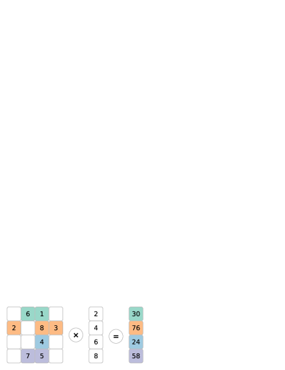
Figure 1: A simple example of SpMV with a $4\times 4$ matrix and a vector. The product of the SpMV is a one-dimensional vector.

II-B Sparse Matrix Representation

Since most of the elements of a sparse matrix are zeros, it would be a waste of space and time to store these entries and perform arithmetic operations on them. To this end, researcher have designed a number of compressed storage representations to store only the nonzeros. We describe the sparse matrix representations targeted in this work. Note that different representations require different SpMV implementations, and thus have different performance on distinct architectures and inputs.

COO. The coordinate (COO) format (a.k.a. IJV format) is a particularly simple storage scheme. The arrays row, col, and data are used to store the row indices, column indices, and values of the nonzeros. This format is a general sparse matrix representation, because the required storage is always proportional to the number of nonzeros for any sparsity pattern. Different from other formats, COO stores explicitly both row indices and column indices. Table I shows an example matrix in the COO format.

TABLE I: Matrix storage formats and their data structures for the sparse matrix shown in Figure 1.

Representation	Specific Values
COO	$row=[0,0,1,1,1,2,3,3]$ $col=[1,2,0,2,3,2,1,2]$ $data=[6,1,2,8,3,4,7,5]$
CSR	$ptr=[0,2,5,6,8]$ $indices=[1,2,0,2,3,2,1,2]$ $data=[6,1,2,8,3,4,7,5]$
CSR5	$ptr=[0,2,5,6,8]$ $tile\_ptr=[0,1,4]$ $tile\_des:bit\_flag=[T,T,F,F|T,T,T,F],$ $y\_off=[0,1|0,2],seg\_off=[0,0|0,0]$ $indices=[1,0,2,2|3,1,2,2]$ $data=[6,2,1,8|3,7,4,5]$
ELL	$data=\begin{bmatrix}6&1&*\\ 2&8&3\\ 4&*&*\\ 7&5&*\end{bmatrix}$ $indices=\begin{bmatrix}1&2&*\\ 0&2&3\\ 2&*&*\\ 1&2&*\end{bmatrix}$
SELL	$data=\begin{bmatrix}6&1&*\\ 2&8&3\\ 4&*&\\ 7&5&\end{bmatrix}$ $indices=\begin{bmatrix}1&2&*\\ 0&2&3\\ 2&*&\\ 1&2&\end{bmatrix}$ $slices=[3,2]$
SELL-C-$\sigma$	$data=\begin{bmatrix}2&8&3\\ 6&1&*\\ 7&5&\\ 4&*&\\ \end{bmatrix}$ $indices=\begin{bmatrix}0&2&3\\ 1&2&*\\ 1&2&\\ 2&*&\\ \end{bmatrix}$ $slices=[3,2]$
HYB	ELL: $data=\begin{bmatrix}6&1\\ 2&8\\ 4&*\\ 7&5\end{bmatrix}$ $indices=\begin{bmatrix}1&2\\ 0&2\\ 2&*\\ 1&2\end{bmatrix}$ COO: $row=[1]$, $col=[3]$, $data=[3]$

CSR. The compressed sparse row (CSR) format is the most popular, general-purpose sparse matrix representation. This format explicitly stores column indices and nonzeros in array indices and data, and uses a third array ptr to store the starting nonzero index of each row in the sparse matrix (i.e., row pointers). For an $M\times N$ matrix, ptr is sized of $M+1$ and stores the offset into the $i^{th}$ row in ptr[i]. Thus, the last entry of ptr is the total number of nonzeros. Table I illustrates an example matrix represented in CSR. We see that the CSR format is a natural extension of the COO format by using a compressed scheme. In this way, CSR can reduce the storage requirement. More importantly, the introduced ptr facilitates a fast query of matrix values and other interesting quantities such as the number of nonzeros in a particular row.

CSR5. To achieve near-optimal load balance for matrices with any sparsity structures, CSR5 first evenly partitions all nonzero entries to multiple 2D tiles of the same size. Thus when executing parallel SpMV operation, a compute core can consume one or more 2D tiles, and each SIMD lane of the core can deal with one column of a tile. Then the main skeleton of the CSR5 format is simply a group of 2D tiles. The CSR5 format has two tuning parameters: $\omega$ and $\sigma$, where $\omega$ is a tile’s width and $\sigma$ is its height. CSR5 is an extension to the CSR format [21]. Apart from the three data structures from CSR, CSR5 introduces another two data structures: a tile pointer tile_ptr and a tile descriptor tile_des. Table I illustrates an example matrix represented in CSR5, where $\omega$=$\sigma$=$2$.

ELL. The ELLPACK (ELL) format is suitable for the vector architectures. For an $M\times N$ matrix with a maximum of $K$ nonzeros per row, ELL stores the sparse matrix in a dense $M\times K$ array (data), where the rows having fewer than $K$ are padded. Another data structure indices stores the column indices and is zero-padded in the same way with that of data. Table I shows the ELL representation of the example sparse matrix, where $K=3$ and the data structures are padded with *. The ELL format would waste a decent amount of storage. To mitigate this issue, we can combine ELL with another general-purpose format such as CSR or COO (see Section I).

SELL and SELL-C-$\sigma$. Sliced ELL (SELL) is an extension to the ELL format by partitioning the input matrix into strips of $C$ adjacent rows [25]. Each strip is stored in the ELL format, and the number of nonzeros stored in ELL may differ over strips. Thus, a data structure slice is used to keep the strip information. Table I demonstrates a matrix represented in the SELL format when $C=2$. A variant to SELL is the SELL-C-$\sigma$ format which introduces sorting to save storage overhead [19]. That is, they choose to sort the matrix rows not globally but within $\sigma$ consecutive rows. Typically, the sorting scope $\sigma$ is selected to be a multiple of $C$. The effect of local sorting is shown in Table I with $C=2$ and $\sigma=4$.

HYB. The HYB format is a combination of ELL and COO, and it stores the majority of matrix nonzeros in ELL while the remaining entries in COO [1]. Typically, HYB stores the typical number of nonzeros per row in the ELL format and the exceptionally long rows in the COO format. In the general case, this typical number ($K$) can be calculated directly from the input matrix. Table I shows an example matrix in this hybrid format, with $K=2$.

III Evaluation Setup

III-A Hardware Platforms

Our work targets two many-core architectures designed for HPC, described as follows.

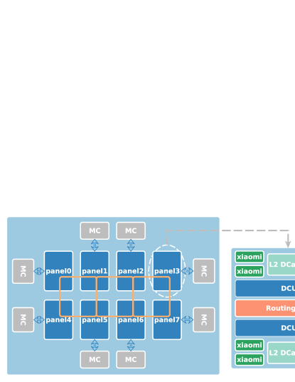
Figure 2: A high-level view of the FT-2000Plus architecture. Processor cores are groups into panels (left) where each panel contains eight ARMv8 based Xiaomi cores (right).

FT-2000Plus. Figure 2 gives a high-level view of the FT-2000Plus architecture. This architecture [29] integrates 64 ARMv8 based Xiaomi cores, offering a peak performance of 512 Gflops for double-precision operations, with a maximum power consumption of 100 Watts. The cores can run up to 2.4 GHz, and are groups into eight panels with eight cores per panel. Each core has a private L1 data cache of 32KB, and a dedicated 2MB L2 cache shared among four cores. The panels are connected through two directory control units (DCU) and a routing cell [50], where cores and caches are linked via a 2D mesh network. External I/O are managed by the DDR4 memory controllers (MC), and the routing cells at each panel link the MCs to the DCUs.

Intel KNL. A KNL processor has a peak performance of 6 Tflops/s and 3Tflops/s respectively for single- and double-precision operations [31]. A KNL socket can have up to 72 cores where each core has four threads running at 1.3 GHz. Each KNL core has a private L1 data and a private L1 instruction caches of 32KB, as well as two vector processor units (VPU), which differs from the KNC core [11, 10].

As shown in Figure 3, KNL cores are organized around 36 tiles where each title has two cores. Each title also has a private, coherent 1MB L2 data cache shared among cores, which is managed by the cache/home agent (CHA). Tiles are connected into a 2D mesh to facilitate coherence among the distributed L2 caches. Furthermore, a KNL chip has a ‘near’ and a ‘far’ memory components. The ‘near’ memory components are multi-channel DRAM (MCDRAM) which are connected to the tiles through the MCDRAM Controllers (EDC). The ‘far’ memory components are DDR4 RAM connected to the chip via the DDR memory controllers (DDR MC). While the ‘near’ memory is smaller than the ‘far’ memory, it provides 5x more bandwidth over traditional DDRs. Depending how the chip is configured, some parts or the entire near memory can share a global memory space with the far memory, or be used as a cache. In this context, MCDRAM is used in the cache mode and the dataset can be hold in the high-speed memory.

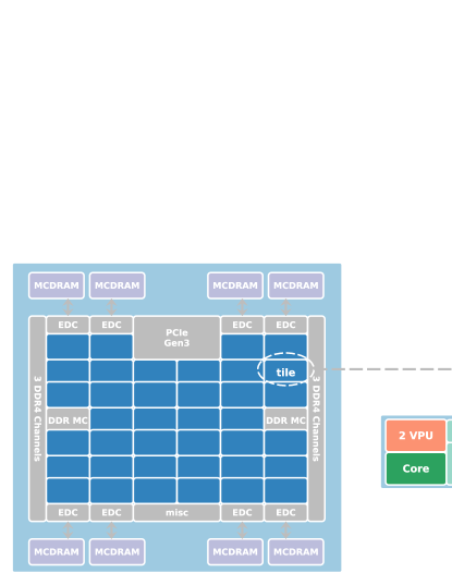
Figure 3: A high-level overview of the Intel KNL architecture. Cores are grouped into tiles (left) with two cores per title (right).

III-B Systems Software

Both platforms run a customized Linux operating system with Kernel v4.4.0 on FTP and v3.10.0 on KNL. For compilation, we use gcc v6.4.0 on FTP and Intel icc v17.0.4 on KNL with the default “-O3” compiler option. We use the OpenMP threading model on both platforms with 64 threads on FTP and 272 threads on KNL.

III-C Datasets

Our experiments use a set of 956 square matrices (with a total size of 90 GB) from the SuiteSparse matrix collection [7]. The number of nonzeros of these matrices ranges from 100K to 20M. The dataset includes both regular and irregular matrices, covering application domains ranging from scientific computing to social networks.

III-D SpMV Implementation

Algorithm 1 illustrates our library-based SpMV implementation using the CSR5 format as an example. Our library takes in the raw data of the Matrix Market format into memory of the COO format. Then we convert the COO-based data into our target storage format (CSR, CSR5, ELL, SELL, or HYB). When calculating SpMV, we use the OpenMP threading model for parallelization. This process is format dependent, i.e., the basic task can be a row, a block row, or a data tile. When calculating a single element of $\mathbf{y}$ falls into different tasks, we will have to gather the partial results. This efficient data gathering can be achieved by manually vectorize the SpMV code with intrinsics. Due to the lack of the gather/scatter function, we do not use the neon intrinsics on FTP. This is because our experimental results show that explicitly using the intrinsics results in a loss in performance, compared with the C version. When measuring the performance, we run the experiments for $FRQ$ times and calculate the mean results.

Algorithm 1 The SpMV Bench based on CSR5

1:procedure BenchSpMV($\mathbf{A}$, $\mathbf{x}$; $\mathbf{y}$)

2:        COOFMT* $ctx$ $\leftarrow$ ReadMatrix($mtx\_file$)

3:        CSR5FMT* $ntx$ $\leftarrow$ ConvertToCSR5($ctx$)

4:        for $t\leftarrow 1,2,\ldots,FRQ$ do

5:               #pragma omp for

6:               for each tile $dt$ in $ntx$ do

7:                       $y^{\prime}$ $\leftarrow$ CalculateSpMV($dt$)

8:               end for

9:               UpdateProduct($y$, $y^{\prime}$)

10:        end for

11:        DumpInfo($runT$, $gflops$, $bw$)

12:        DeleteMTX($ctx$, $ntx$)

13:end procedure

IV Memory Allocation and Code Vectorization

SpMV performance depends on a number of factors on a many-core architecture. These include memory allocation and code optimization strategies, and the sparse matrix representation. The focus of this work is to identify the optimal sparse matrix representation that leads to the quickest running time. To isolate the problem, we need to ensure that performance comparisons of different representations are conducted on the best possible memory allocation and code optimization strategies. To this end, we investigate how Non-Uniform Memory Access (NUMA) and code vectorization affect the SpMV performance on FTP and KNL. We then conduct our experiments on the best-found strategy of NUMA memory allocation and vectorization.

IV-A The Impact of NUMA Bindings

Unlike the default setting of KNL, the FTP architecture exposes multiple NUMA nodes where a group of eight cores are directly connected to a local memory module. Indirect access to remote memory modules is possible but slow. This experiment evaluates the impact of NUMA on SpMV performance on FTP. We use the Linux NUMA utility, numactl, to allocate the required data buffers from the local memory module of a running processor.

Figure 4 show the performance improvement when using NUMA-aware over non-NUMA-aware memory allocation across five sparse matrix representation. We see that static NUMA bindings enables significant performance gains for all the five storage formats on FTP. Compared with the case without tuning, using the NUMA tunings can yield an average speedup of 1.5x, 1.9x, 6.0x, 2.0x, and 1.9x for CSR, CSR5, ELL, SELL, and HYB, respectively. Note that we have achieved the maximum speedup for the ELL-based SPMV. This is due to the fact that using ELL allocates the largest amount of memory buffers, and the manual NUMA tunings can ensure that each NUMA node accesses its local memory as much as possible.

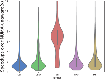
Figure 4: The violin diagram shows the speedup distribution of NUMA-aware memory allocation over NUMA-unaware memory allocation on FTP. The thick black line shows where 50% of the data lie. NUMA-aware memory allocation can significantly improve the SpMV performance.

IV-B The Impact of Vectorization on KNL

The two many-core architectures considered in the work support SIMD vectorization [12]. KNL and FTP have a vector unit of 512 and 128 bits respectively. Figure 5 shows that vectorization performance of CSR5 and SELL-based SpMV on KNL. Overall, we see that manually vectorizing the code using vectorization intrinsics can significantly improve the SpMV performance on KNL. Compared with the code without manual vectorization, the vectorized code yields a speedup of 1.6x for CSR5 and 1.5x for SELL. However, we observe no speedup for vectorized code on FTP. This is that because FTP has no support of the gather operation which is essential for accessing elements from different locations of a vector. By contrast, KNL supports _mm512_i32logather_pd, which improves the speed of the data loading process. Therefore, for the remaining experiments conducted in this work, we manually vectorize the code on KNL but not on FTP.

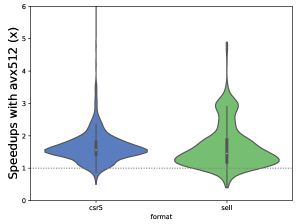
Figure 5: The SpMV performance with and without explicit vectorization on KNL.

IV-C FTP versus KNL

Figure 6 shows the performance comparison between KNL and FTP. In general, we observe that SpMV on KNL runs faster than it on FTP for each format. The average speedup of KNL over FTP is 1.9x for CSR, 2.3x for CSR5, 1.3x for ELL, 1.5x for SELL, and 1.4x for HYB. The performance disparity comes from the difference in the memory hierarchy of the architectures. KNL differs from FTP in that it has a high-speed memory, a.k.a., MCDRAM, between the L2 cache and the DDR4 memory. MCDRAM can provide 5x more memory bandwidth over the traditional DDR memory. Once the working data is loaded into this high-speed memory, the application can then access the data with a higher memory bandwidth which leads to a better overall performance. SpMV on KNL also benefits from the support of gather/scatter operations (see Section IV-B). This is key for the overall SpMV performance, which is limited by the scattered assess of the input vector. To sum up, we would have a significant performance increase when the aforementioned memory features are enabled on FTP.

From Figure 6, we also observe FTP outperforms KNL on some matrices, specially when the size of the input matrices is small. The performance disparity is due to the fact that KNL and FTP differ in L2 cache in terms of both capacity and coherence protocol.

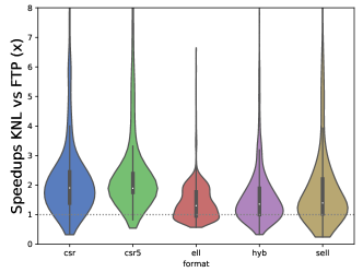
Figure 6: Comparing the SpMV performance between KNL and FTP. The x-axis labels different sparse matrix representation, and the y-axis denotes the achieved speedup of KNL over FTP.

TABLE II: The best format distribution on FTP and KNL.

	CSR	CSR5	ELL	SELL	HYB
FTP	127(14.1%)	149(16.5%)	22(2.4%)	443(49.2%)	160(17.6%)
KNL	493(51.8%)	273(28.7%)	39(4.1%)	121(12.7%)	25(2.6%)

(a) On FTP with 64 threads

(b) On KNL with 272 threads

Figure 7: The overall performance of SpMV on FTP and KNL. The x-axis labels different sparse matrices ordered by the number of nonzeros, and the y-axis denotes the achieved SpMV performance in GFlops.

TABLE III: The average slowdowns over all the matrices when using a single format instead of the individual best.

	CSR	CSR5	ELL	SELL	HYB
FTP	1.4x	1.8x	6.4x	1.3x	1.3x
KNL	1.3x	1.4x	8.7x	1.5x	1.6x

IV-D Optimal Sparse Matrix Formats

Figure 7 shows the overall performance of SpMV on FTP and KNL . We see that there is no “one-size-fits-all” format across inputs and architectures. On the FTP platform, SELL is the optimal format for around 50% of the sparse matrices and ELL gives the worse performance on most of the cases. On the KNL platform, CSR gives the best performance for most of the cases, which is followed by CSR5 and SELL. On KNL, ELL and HYB give the best performance for just a total of 64 sparse matrices (Table II).

Table III shows the average slowdowns when using a fixed format across test cases over the optimal one. The slowdown has a negative correlation with how often a given format being optimal. For example, CSR gives the best overall performance on KNL and as such it has the lowest overall slowdown. Furthermore, SELL and HYB have a similar average slowdown on FTP because they often deliver similar performance (see Figure 7(a)).

Given that the optimal sparse matrix storage format varies across architectures and inputs, finding the optimal format is a non-trivial task. What we like to have is an adaptive scheme that can automatically choose the right format for a given input and architecture. In the next section, we describe how to develop such a scheme using machine learning.

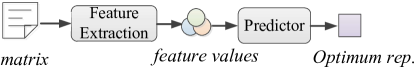
Figure 8: Overview of our approach.

V Adaptive Representation Selection

V-A Overall Methodology

Our approach takes a new, unseen sparse matrix and is able to predict the optimal or near optimal sparse matrix representation for a given architecture. An overview of our approach can be seen in Figure 8, and is described in more details in Section V-B. Our predictive model is built upon the scikit-learn machine learning package [28].

For a given sparse matrix, our approach will collect a set of information, or features, to capture the characteristics of the matrix. The set of feature values can be collected at compile time or during runtime. Table IV presents a full list of all our considered features. After collecting the feature values, a machine learning based predictor (that is trained offline) takes in the feature values and predicts which matrix representation should be used for the target architecture. We then transform the matrix to the predicted format and generate the computation code for that format.

V-B Predictive Modeling

Our model for predicting the best sparse matrix representation is a decision tree model. We have evaluated a number of alternate modelling techniques, including regression, Naive Bayes and K-Nearest neighbour (see also Section V-D). We chose the decision tree model because it gives the best performance and can be easily interpreted compared to other black-box models. The input to our model is a set of features extracted from the input matrix. The output of our model is a label that indicates which sparse matrix representation to use.

Building and using such a model follows the 3-step process for supervised machine learning: (i) generate training data (ii) train a predictive model (iii) use the predictor, described as follows.

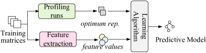
Figure 9: The training process of our predictive model.

V-B1 Training the Predictor

Our method for training the predictive model is shown in Figure 9. We use the same approach to train a model for each targeting architecture. To train a predictor we first need to find the best sparse matrix representation for each of our training matrix examples, and extract features. We then use this set of data and classification labels to train our predictor model.

Generating Training Data. We use five-fold-cross validation for training. This standard machine learning technique works by selecting 20% samples for testing and using 80% samples for training. To generate the training data for our model we used 756 sparse matrices from the SuiteSparse matrix collection. We execute SpMV using each sparse matrix representation a number of times until the gap of the upper and lower confidence bounds is smaller than 5% under a 95% confidence interval setting. We then record the best-performing matrix representation for each training sample on both KNL and FTP. Finally, we extract the values of our selected set of features from each matrix.

Building The Model. The optimal matrix representation labels, along with their corresponding feature set, are passed to our supervised learning algorithm. The learning algorithm tries to find a correlation between the feature values and optimal representation labels. The output of our learning algorithm is a version of our decision-tree based model. Because we target two platforms in this paper, we have constructed two predictive models, one model per platform. Since training is performed off-line and only need to be carried out once for a given architecture, this is a one-off cost.

Total Training Time. The total training time of our model is comprised of two parts: gathering the training data, and then building the model. Gathering the training data consumes most of the total training time, in this paper it took around 3 days for the two platforms. In comparison actually building the model took a negligible amount of time, less than 10 ms.

V-B2 Features

One of the key aspects in building a successful predictor is developing the right features in order to characterize the input. Our predictive model is based exclusively on static features of the target matrix and no dynamic profiling is required. Therefore, it can be applied to any hardware platform. The features are extracted using our own Python script. Since our goal is to develop a portable, architecture-independent approach, we do not use any hardware-specific features [9].

Feature Selection. We considered a total of seven candidate raw features (Table IV) in this work. Some features were chosen from our intuition based on factors that can affect SpMV performance e.g. nnz_frac and variation, other features were chosen based on previous work [33]. Altogether, our candidate features should be able to represent the intrinsic parts of a SpMV kernel.

TABLE IV: The features used in our model.

Features	Description
n_rows	number of rows
n_cols	number of columns
nnz_frac	percentage of nonzeros
nnz_min	minimum number of nonzeros per row
nnz_max	maximum number of nonzeros per row
nnz_avg	average number of nonzeros per row
nnz_std	standard derivation of nonzeros per row
variation	matrix regularity

Feature Scaling. The final step before passing our features to a machine learning model is scaling each scalar value of the feature vector to a common range (between 0 and 1) in order to prevent the range of any single feature being a factor in its importance. Scaling features does not affect the distribution or variance of their values. To scale the features of a new image during deployment we record the minimum and maximum values of each feature in the training dataset, and use these to scale the corresponding features.

V-B3 Runtime Deployment

Deployment of our predictive model is designed to be simple and easy to use. To this end, our approach is implemented as an API. The API has encapsulated all of the inner workings, such as feature extraction and matrix format translation. We also provide a source to source translation tool to transform the computation of a given SpMV kernel to each of target representations. Using the prediction label, a runtime can choose which SpMV kernel to use.

V-C Predictive Model Evaluation

We use cross-validation to evaluate our approach. Specially, we randomly split the 965 matrices into two parts: 756 matrices for training and 200 matrices for testing. We learn a model with the training matrices and five representations. We then evaluate the learned model by applying it to make prediction on the 200 testing matrices. We repeat this process multiple times to ensure each matrix is tested at least once.

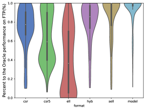
(a) FTP

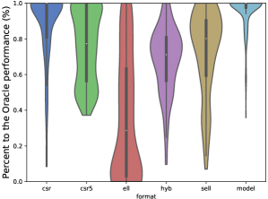
(b) KNL

Figure 10: The predicted performance of SpMV on FTP and KNL. We show the achieved SpMV performance with respect to the best available performance across sparse matrix format.

Figure 10 shows that our predictor achieves, on average, 91% and 95% of the best available SpMV performance (found through exhaustive search) on FTP and KNL respectively. It outperforms a strategy that uses only a single format. As we have analyzed in Table III, SELL and HYB can achieve a better performance than the other three formats on FTP. But they are still overtaken by our predictor. On KNL, however, the performance of our predictor is followed by using the CSR representation. Also, we note that using the ELL representation yields poor performance on both FTP and KNL. This shows that our predictor is highly effective in choosing the right sparse matrix representation.

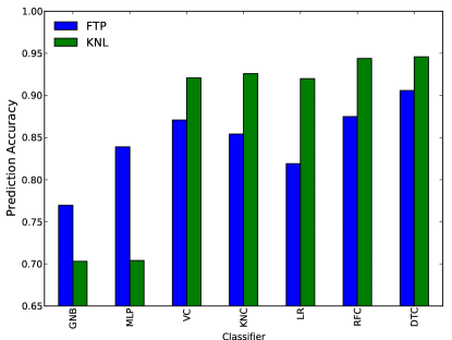
Figure 11: Compare to alternative modeling techniques

V-D Alternative Modeling Techniques

Figure 11 shows resulting performance with respect to the best available performance when using different techniques to construct the predictive model. In addition to our decision tree based model (DTC), we also consider Gaussian naïve bayes (GNB), multilayer perception (MLP), soft voting/majority rule Classification (VC), k-Nearest Neighbor (KNC, k=1), logistic regression (LR), random forests classification (RFC). Thanks to the high-quality features, all classifiers are highly accurate in choosing sparse matrix representation. We choose DTC because its accuracy is comparable to alternative techniques and can be easily visualized and interpreted.

VI Related Work

SpMV has been extensively studied on various platforms over the past few decades [24, 30, 46]. A large body of work has been dedicated to efficient and scalable SpMV on multi-core and many-core processors. However, our work is the first to conduct a comprehensive study on KNL and FTP.

On the SIMD processors., some researchers have designed new compressed formats to enable efficient SpMV [47, 1, 13, 17, 46]. Liu et al. propose a storage format CSR5 [21], which is a tile-based format. CSR5 offers high-throughput SpMV on various platforms and shows good performance for both regular and irregular matrices. And the format conversion from CSR to CSR5 can be as low as the cost of a few SpMV operations. On KNC, Liu et al. have identified and addressed several bottlenecks [22]. They exploit the salient architecture features of KNC, use specialized data structures with careful load balancing to obtain satisfactory performance. Wai Teng Tang et al. propose a SpMV format called vectorized hybrid COO+CSR (VHCC) [35], which employs a 2D jagged partitioning, tiling and vectorized prefix sum computations to improve hardware resource. Their SpMV implementation achieves an average 3x speedup over Intel MKL for a range of scale-free matrices.

In recent years, ELLPACK is the most successful format on the wide SIMD processors. Bell and Garland propose the first ELLPACK-based format HYB, combining ELLPACK with COO formats [1]. The HYB can improve the SpMV performance especially for matrix which are “wide”. Sliced ELLPACK format has been proposed by Monakov et al., where slices of the matrix are packed in ELLPACK format separately [25]. BELLPACK is a format derived from ELLPACK, which sorts rows of the matrix by the number of nonzeros per row [5]. Monritz Kreutzer et al. have designed a variant of Sliced ELLPACK SELL-C-sigma based on Sliced ELLPACK as a SIMD-friendly data format, in which slices are sorted [19].

There have also been studies on optimizing SpMV dedicated for SIMT GPUs [23, 1, 39, 35]. Wai Teng Tang et al. introduce a series of bit-representation-optimized compression schemes for representing sparse matrices on GPUs including BRO-ELL, BRO-COO, BRO-HYB, which perform compression on index data and help to speed up SpMV on GPUs through reduction of memory traffic [34]. Jee W. Choi et al. propose a classical blocked compressed sparse row (BCSR) and blocked ELLPACK (BELLPACK) storage formats [5], which can match or exceed state-of-the-art implementations. They also develop a performance model that can guide matrix-dependent parameter tuning which requires offline measurements and run-time estimation modelling the architecture of GPUs. Yang et al. present a novel non-parametric and self-tunable approach [49] to data presentation for computing this kernel, particularly targeting sparse matrices representing power-law graphs. They take into account the skew of the non-zero distribution in matrices presenting power-law graphs.

Sparse matrix storage format selection. is required because various formats have been proposed for diverse application scenarios and computer architectures [52]. In [33], Sedaghat et al. study the inter-relation between GPU architectures, sparse matrix representation, and the sparse dataset. Further, they build a model based on decision tree to automatically select the best representation for a given sparse matrix on a given GPU platform. The decision-tree technique is also used in [20], where Li et al. develop a sparse matrix-vector multiplication auto-tuning system to bridge the gap between specific optimizations and general-purpose usage. This framework provides users with a unified programming interface in the CSR format and automatically determines the optimal format and implementation for any input sparse matrix at runtime. In [52], Zhao et al. propose to use the deep learning technique to select a right storage format. Compared to the traditional machine learning techniques, using deep learning can avoid the difficulties in coming up with the right features of matrices for the purpose of learning. The results have shown that the CNN-based technique can cut format selection errors by two thirds.

Predictive Modeling. Machine learning has been employed for various optimization tasks [42], including code optimization [41, 38, 43, 44, 16, 45, 40, 36, 26, 6, 27, 51], task scheduling [14, 8, 15, 32], model selection [37], etc.

Although SpMV optimization has been extensively studied, it remains unclear how the widely-used sparse matrix representations perform on the emerging many-core architectures. Our work aims to bridge this gap by providing an in-depth analysis on two emerging many-core architectures (KNL and FTP), with a large number of sparse matrices and five well-recognized storage formats. Our work is the first attempt in applying machine learning techniques to optimize SpMV on KNL and FTP.

VII Conclusion

This paper has presented a comprehensive study of SpMV performance on two emerging many-core architectures using five mainstream matrix representations. We study how the NUMA binding, vectorization, and the SpMV storage representation affect the runtime performance. Our experimental results show that the best-performing sparse matrix representation depends to the underlying architectures and the sparsity patterns of the input datasets. To facilitate the selection of the best representation, we use machine learning to automatically learn a model to predict the right matrix representation for a given architecture and input. Our model is first trained offline and the learned model can be used for any unseen input matrix. Experimental results show that our model is highly effective in selecting the matrix representation, delivering over 90% of the best available performance on our evaluation platforms.

References

- [1] Nathan Bell and Michael Garland. Implementing sparse matrix-vector multiplication on throughput-oriented processors. In SC, 2009.
- [2] Yonggang Che et al. Realistic performance characterization of CFD applications on intel many integrated core architecture. Comput. J., 2015.
- [3] Jing Chen et al. Efficient and portable ALS matrix factorization for recommender systems. In IPDPS, 2017.
- [4] Jing Chen et al. clmf: A fine-grained and portable alternating least squares algorithm for parallel matrix factorization. FGCS, 2018.
- [5] JeeWhan Choi et al. Model-driven autotuning of sparse matrix-vector multiply on gpus. In PPoPP, 2010.
- [6] Chris Cummins et al. End-to-end deep learning of optimization heuristics. In PACT, 2017.
- [7] Timothy A. Davis and Yifan Hu. The university of florida sparse matrix collection. ACM Trans. Math. Softw., 2011.
- [8] Murali Krishna Emani et al. Smart, adaptive mapping of parallelism in the presence of external workload. In CGO, 2013.
- [9] Jianbin Fang et al. An auto-tuning solution to data streams clustering in opencl. In CSE, 2011.
- [10] Jianbin Fang et al. An empirical study of intel xeon phi. CoRR, 2013.
- [11] Jianbin Fang et al. Test-driving intel xeon phi. In ICPE, 2014.
- [12] Jianbin Fang and otherss. Evaluating vector data type usage in opencl kernels. Concurrency and Computation: Practice and Experience, 2015.
- [13] Georgios I. Goumas et al. Performance evaluation of the sparse matrix-vector multiplication on modern architectures. The Journal of Supercomputing, 2009.
- [14] Dominik Grewe et al. A workload-aware mapping approach for data-parallel programs. In HiPEAC, 2011.
- [15] Dominik Grewe et al. Opencl task partitioning in the presence of gpu contention. In LCPC, 2013.
- [16] Dominik Grewe et al. Portable mapping of data parallel programs to opencl for heterogeneous systems. In CGO, 2013.
- [17] Eun-Jin Im et al. Sparsity: Optimization framework for sparse matrix kernels. IJHPCA, 2004.
- [18] D.R. Kincaid et al. Itpackv 2d user’s guide. Technical report, Center for Numerical Analysis, Texas Univ., Austin, TX (USA), 1989.
- [19] Moritz Kreutzer et al. A unified sparse matrix data format for efficient general sparse matrix-vector multiplication on modern processors with wide SIMD units. SIAM J. Scientific Computing, 2014.
- [20] Jiajia Li et al. SMAT: an input adaptive auto-tuner for sparse matrix-vector multiplication. In PLDI, 2013.
- [21] Weifeng Liu and Brian Vinter. CSR5: an efficient storage format for cross-platform sparse matrix-vector multiplication. In ICS, 2015.
- [22] Xing Liu et al. Efficient sparse matrix-vector multiplication on x86-based many-core processors. In ICS, 2013.
- [23] Marco Maggioni and Tanya Y. Berger-Wolf. An architecture-aware technique for optimizing sparse matrix-vector multiplication on gpus. In ICCS, 2013.
- [24] John M. Mellor-Crummey and John Garvin. Optimizing sparse matrix - vector product computations using unroll and jam. IJHPCA, 2004.
- [25] Alexander Monakov et al. Automatically tuning sparse matrix-vector multiplication for GPU architectures. In HIPEAC, 2010.
- [26] William F Ogilvie et al. Fast automatic heuristic construction using active learning. In LCPC, 2014.
- [27] William F Ogilvie et al. Minimizing the cost of iterative compilation with active learning. In CGO, 2017.
- [28] F. Pedregosa et al. Scikit-learn: Machine learning in Python. Journal of Machine Learning Research, 2011.
- [29] Phytium Technology Co. Ltd. FT-2000, February 2017. http://www.phytium.com.cn/Product/detail?language=1&product_id=7.
- [30] Ali Pinar and Michael T. Heath. Improving performance of sparse matrix-vector multiplication. In SC, 1999.
- [31] Sabela Ramos and Torsten Hoefler. Capability models for manycore memory systems: A case-study with xeon phi KNL. In IPDPS, 2017.
- [32] Jie Ren et al. Optimise web browsing on heterogeneous mobile platforms: a machine learning based approach. In INFOCOM, 2017.
- [33] Naser Sedaghati et al. Automatic selection of sparse matrix representation on gpus. In ICS, 2015.
- [34] Wai Teng Tang et al. Accelerating sparse matrix-vector multiplication on gpus using bit-representation-optimized schemes. In SC, 2013.
- [35] Wai Teng Tang et al. Optimizing and auto-tuning scale-free sparse matrix-vector multiplication on intel xeon phi. In CGO, 2015.
- [36] Ben Taylor et al. Adaptive optimization for opencl programs on embedded heterogeneous systems. In LCTES, 2017.
- [37] Ben Taylor et al. Adaptive deep learning model selection on embedded systems. In LCTES, 2018.
- [38] Georgios Tournavitis et al. Towards a holistic approach to auto-parallelization: Integrating profile-driven parallelism detection and machine-learning based mapping. In PLDI, 2009.
- [39] Anand Venkat et al. Non-affine extensions to polyhedral code generation. In CGO, 2014.
- [40] Zheng Wang et al. Automatic and portable mapping of data parallel programs to opencl for gpu-based heterogeneous systems. ACM TACO, 2014.
- [41] Zheng Wang et al. Integrating profile-driven parallelism detection and machine-learning-based mapping. ACM TACO, 2014.
- [42] Zheng Wang and Michael O’Boyle. Machine learning in compiler optimisation. Proc. IEEE, 2018.
- [43] Zheng Wang and Michael F.P. O’Boyle. Mapping parallelism to multi-cores: A machine learning based approach. In PPoPP, 2009.
- [44] Zheng Wang and Michael FP O’Boyle. Partitioning streaming parallelism for multi-cores: a machine learning based approach. In PACT, 2010.
- [45] Zheng Wang and Michael FP O’boyle. Using machine learning to partition streaming programs. ACM TACO, 2013.
- [46] Samuel Williams et al. Optimization of sparse matrix-vector multiplication on emerging multicore platforms. In SC, 2007.
- [47] Samuel Williams et al. Optimization of sparse matrix-vector multiplication on emerging multicore platforms. Parallel Computing, 2009.
- [48] Xi Yang et al. High performance coordinate descent matrix factorization for recommender systems. In CF, 2017.
- [49] Xintian Yang et al. Fast sparse matrix-vector multiplication on gpus: Implications for graph mining. PVLDB, 2011.
- [50] Charles Zhang. Mars: A 64-core armv8 processor. In HotChips, 2015.
- [51] Peng Zhang et al. Auto-tuning streamed applications on intel xeon phi. In IPDPS, 2018.
- [52] Yue Zhao et al. Bridging the gap between deep learning and sparse matrix format selection. In PPoPP, 2018.