gray 1gray1

On the Mathematics of Higher Structures

1. Introduction

In a series of papers [10, 9, 17, 15, 7, 8, 16, 5, 6, 4, 14, 3, 2, 12, 11, 13, 18] we have discussed higher structures in science in general, and developed a framework called Hyperstructures for describing and working with higher structures. In [12] we discussed the philosophy behind higher structures and formulated a principle in six stages — the Hyperstructure Principle — for forming higher structures.

In this paper we will relate hyperstructures and the general principle to known mathematical structures. We also discuss how they may give rise to new mathematical structures and prepare a framework for a mathematical theory.

Let us first recall from [12] what we think is the basic principle in forming higher structures.

2. The $\mathscr{H}$-Principle

• Observation and Detection.
  

  Given a collection of objects that we want to study and give a structure. First we observe the objects and detect or assign their properties, states, etc. This is the semantic part of the process. Finally we may also select special objects.
  

• Binding.
  

  A procedure to produce new objects from collections of old objects by “binding” them in some way. This is the syntactic part of the process.
  

• Levels.
  

  Iterating the described process in the following way: forming bonds of bonds and — important! — using the detected and observed properties at one level in forming the next level. This is iteration in a new context and not a recursive procedure. It combines syntax and semantics in forming a new level. Connections between levels are given by specifying how to dissolve a bond into lower level objects. When bonds have been formed to constitute a new level, observation and detection are like finding “emergent properties” of the process.
  

These three steps are the most important ones, but we include three more in the general principle.

• Local to global.
  

  Describing a procedure of how to move from the bottom (local) level through the intermediate levels to the top (global) level with respect to general properties and states. The importance of the level structure lies in the possibility of manipulating the systems levelwise in order to achieve a desired global goal or state. This can be done using “globalizers” — an extension of sections in sheaves on Grothendieck sites (see [9]).
  

• Composition.
  

  A way to produce new bonds from old ones. This means that we can compose and produce new bonds on a given level, by “gluing” (suitably interpreted) at lower levels. The rules may vary and be flexible due to the relevant context.
  

• Installation.
  

  Putting a level structure satisfying I–V on a set or collection of objects in order to perform an analysis, synthesis or construction in order to achieve a given goal. The objects to be studied may be introduced as bonds (top or bottom) in a level structure.
  

  Synthesis: The given collection is embedded at the bottom level.
  

  Analysis: The given collection is embedded at the top level.
  

Synthesis facilitates local to global processes and dually, analysis facilitates global to local processes by defining localizers dual to globalizers, see [10].

The steps I–VI are the basic ingredients of what we call the Hyperstructure Principle or in short the $\mathscr{H}$-principle. (Corresponding to “The General Principle” in [4].) In our opinion it reflects the basic way in which we make or construct things.

Let us illustrate this in terms of category theory:

1. Observation and detection: we decide the structure of the objects like topological spaces, groups, etc.
   

2. Binding: morphisms bind objects — in an ordered way, continuous maps, homomorphisms, etc.
   

3. Levels: we consider morphisms of morphisms of $\ldots$ in forming higher categories. Observation, detection and assignment become more indirect, but ought to play a more significant role.
   

4. Local to global: at one level think of a Grothendieck sheaf on a site.
   

5. Composition: composition of morphisms etc. in the ordinary sense.
   

6. Installation: giving a collection of objects (like “all groups”) a categorical structure.

3. A categorical implementation of the $\mathscr{H}$-principle

In order to illustrate how the $\mathscr{H}$-principle may be applied in an ordinary categorical setting we take the following example from [4]:

Let $\mathscr{C}$ be a category and $P:\mathscr{C}^{\text{op}}\to\mathrm{Sets}$ a functor called a presheaf. The category of elements of $P$, denoted by

$$\int_{\mathscr{C}}P\;\;,$$

is given as follows.

Objects:

$(C,p)$ where $C$ is an object in $\mathscr{C}$ and $p\in P(C)$.

Morphisms:

$(C^{\prime},p^{\prime})\to(C,p)$ are the morphisms $u\colon C^{\prime}\to C$ in $\mathscr{C}$ such that $Pu\colon P(C)\to P(C^{\prime})$ and $Pu(p)=p^{\prime}$.

For this construction see [22].

Then a possible way to contruct a categorical hyperstructure is as follows: Start with a collection of objects $X_{0}$.

Observation:

$$X_{0}\rightsquigarrow \;\mathscr{C}_{0}$$

$$-$$ category

$$\mathscr{C}_{0}\rightsquigarrow \;\mathscr{C}_{0}\text{ or}$$

$$\;\mathrm{Sets}^{\mathscr{C}^{\text{op}}}$$

$$\;\mathscr{C}_{0}^{J}$$

$$\;\vdots$$

$$\Omega_{0}\colon\mathscr{C}_{o}^{\text{op}}\to \;\mathrm{Sets}\text{ (Spaces, categories or other structures)}$$

$$-$$ presheaf

Binding:

$$\Gamma_{0}= \;\int_{\mathscr{C}_{0}}\Omega_{0}$$

$$-$$ category of elements

$$B_{0}\colon\Gamma_{0}^{\text{op}}\to \;\mathrm{Sets}\text{ (Spaces,$\ldots$)}$$

$$-$$ presheaf

Levels:

$$\mathscr{C}_{1}=\int_{\Gamma_{0}}B_{0}$$

Iterating this process by making the appropriate choices we get a hyperstructure:

$$\mathscr{H}=\{\mathscr{C}_{0},\mathscr{C}_{1},\ldots,\mathscr{C}_{n}\}$$

where

$$\mathscr{C}_{m} =\int_{\Gamma_{m-1}}B_{m-1}$$

$$=\underset{\underset{\mathscr{C}_{m-1}}{\int}\Omega_{m-1}}{\int}B_{m-1}$$

for $1\leqslant m<n$.

In category theory it is often very useful to apply the nerve construction to a category (even higher ones) in order to associate a space from which topological information can be extracted. In the present construction the “nerve” of $\mathscr{H}$ would mean the nerve of $\mathscr{C}_{n}$ constructed inductively. The point to be made is that the $\operatorname{Nerve}(\mathscr{H})=|\mathscr{H}|$ makes sense and may be useful in this context.

4. From morphisms to bonds

In category theory we consider an ordered pair of objects $(X,Y)$ and assign a set $\operatorname{Mor}(X,Y)$ of morphisms. Intuitively the morphisms bind the objects together. We suggest to extend the picture to a collection of objects $\mathscr{C}=\{X_{i}\}_{i\in I}$.

The collection could be ordered or non-ordered. We prefer to present here the ideas in the non-ordered case. Hence we assign a set of bonds to the collection

$$B=B(\mathscr{C}).$$

$B$ may sometimes be empty.

The elements are mechanisms “binding” the collection in some way — extending morphisms. Let us look at some examples.

Relations

A relation $R\subseteq X_{1}\times\cdots\times X_{n}$ gives a bond of tuples of elements $R(x_{1},\ldots,x_{n})$ if and only if $(x_{1},\ldots,x_{n})\in R$.

Hypergraphs

Here we are given a set of vertices and the edges are subsets of vertices, and they serve as bonds of these vertices.

Subspaces

Even more general, let $A_{i}$, $i=1,\ldots,n$ be suitable subspaces of $X$ and $A_{i}\subseteq X$. $X$ is then a bond of $\{A_{i}\}$. An interesting case is when $A_{i}$ and $X$ are open subsets of a larger space $Y$.

Simplicial complexes

Given a simplicial complex $K$ based on vertices $\{v_{0},\ldots,v_{q}\}$. Then the simplices may be interpreted as bonds.

Cobordisms

Let $W,\{V_{i}\}_{i=1,\ldots,k}$ be manifolds such that $\partial W=\cup V_{i}$ ($V_{i}$ are the boundary components). We will then call $W$ a bond of $\{V_{i}\}$.

The basic idea:

Instead of assigning a set $\operatorname{Mor}(X,Y)$ to every ordered pair of objects, we will assign a set of bonds to any collection of objects — finite, infinite or uncountable:

$$\operatorname{Bond}(X,Y,Z,\ldots)\quad\text{or}\quad\operatorname{Bond}(c\in\mathscr{C})$$

$\mathscr{C}$ being a collection or parametrized family of objects. We may also consider ordered collections or collections with other additional properties. Bonds extend morphisms in categories and higher bonds create levels and extend higher morphisms (natural transformations and homotopies, etc.) in higher categories. This will be the basis for the creation of new global states.

Bonds are more general than these examples. But prior to the bond assignment is the process of observation, detection and assignment of properties like: manifolds, subspaces, points, vertices, etc. This will become more important when forming levels. Before studying level formation we will discuss property and bond assignments.

Why do we need such an extension from graphs, higher categories, etc. to hyperstructures? In previous papers [10, 9, 17, 15, 7, 8, 16, 5, 6, 4, 14, 3, 2, 12, 11, 13, 18] — to which we refer the reader — we have given many examples to illustrate this: higher order links, higher cobordisms and many more examples where we have group interactions instead of just pair interactions. The essence is that many multiagent interactions require a hyperstructure framework.

Here we just refer to these previous papers for examples and motivation since our goal here is to discuss what we consider is the essence of a philosophy of the mathematics of higher structures — outlining the possibilities for new constructions to be carried out in the future.

5. Property and bond assignments

Properties

By properties here we include: properties, states, phases, etc. Collections we consider as subsets of some given set $X$, meaning that a collection $S\in\mathscr{P}(X)$ — the power set of $X$. In many situations one may just consider structured subsets of $\mathscr{P}(X)$, but the ideas remain the same. Similar to the example in Section 3. We may consider $\mathscr{P}(X)$ as a category with inclusions as morphisms in some cases.

Even if the $\Omega$’s and $B$’s (to be defined later in this section) are just general assignments we may ask how they behave with respect to unions and intersections — even if they are not functors. We may look for analogues of pullback and pushout preservation. In many cases we do not find this and it may lead to new kinds of mathematical structures. This applies to both $\Omega$ and $B$ assignments.

We consider assignments

$$\Omega\colon\mathscr{P}(X)\to\mathrm{Sets}$$

(or having target something more general like a higher category). Should $\Omega$ be a functor, meaning that

$$S^{\prime}\subseteq S$$

implies (contravariantly)

$$\Omega(S^{\prime})\leftarrow\Omega(S)$$

or (covariantly)

$$\Omega(S^{\prime})\to\Omega(S)?$$

In many situations this would be natural.

What about

$$\Omega(S^{\prime}\cup S)$$

in terms of $\Omega(S^{\prime})$ and $\Omega(S)$ where certainly $S^{\prime}\cap S=\emptyset$ is allowed?

Figure 1. Collections for state and bond assignments.

How does $\Omega(S_{1}\cup S_{2})$ relate to $\Omega(S_{1})$, $\Omega(S_{2})$ and $\Omega(S_{1}\cap S_{2})$?

1. If $\Omega$ is a covariant functor then

   (where $\Omega(S_{1}\cup S_{2})=\Omega(S_{1})\sqcup_{\Omega(S_{1}\cap S_{2})}\Omega(S_{2})$) which in some situations may be required to be a pushout.

   If $\Omega$ is contravariant, we may require a pullback:

   But there are situations in the general setting where none of these conditions are satisfied. We need to go beyond (co)-presheaves.

2. In some situations one may require a function or assignment $\varphi$ such that

   $$\Omega(S_{1}\cup S_{2})=\varphi\bigl{(}\Omega(S_{1}),\Omega(S_{2}),\Omega(S_{1}\cap S_{2})\bigl{)}.$$

   $\varphi$ may be thought of as a generalized limit in particular in the case of a union of an arbitrary collection of $S$’s.

   Properties or elements in $\Omega(S_{1}\cup S_{2})$ not in or coming from $\Omega(S_{1})$ or $\Omega(S_{2})$ may be thought of as “emergent” properties.

The theory should be developed in both the cases 1 and 2. In general the only assignment of “emergent” properties is by “observation” — “the whole is more than the sum of its parts.”

Bonds

We now consider collections $S$ with a property $\omega$, $\omega\in\Omega(S)$ and form

$$\Gamma=\{(S,\omega)\mid\omega\in\Omega(S)\}.$$

We want to study the “mechanisms” that can bind the elements of $S$ together to some kind of unity. This is done by an assignment

$$B\colon\Gamma\to\mathrm{Sets},$$

where $B(S,\omega)$ is the set of bonds of $S$.

If $\Omega$ and $B$ are both functors we proceed by known mathematical tools. If one of them or both fail to be functors we need to develop new mathematical methods.

If

it is sometimes natural to require that

is a pushout, or

a pullback. But sometimes these conventional notions fail and one may proceed in different ways.

Bonds ($B$) (like morphisms) represent the syntactic part of the structure. Observation ($\Omega$) — missing in (Higher) Category Theory — represent the semantic part.

For property assignments $\Omega$ we may introduce operations: Given $(S_{1},\omega_{1})$ and $(S_{2},\omega_{2})$, $\omega_{1}\in\Omega(S_{1})$ and $\omega_{2}\in\Omega(S_{2})$, we may define

$$\omega_{1}\circ\omega_{2}=\varphi(\omega_{1},\omega_{2})\in\Omega(S_{1}\cup S_{2}),\quad\text{for $S_{1}$ and $S_{2}$ disjoint.}$$

Whenever a tensor product exists we may require:

$$\Omega(S_{1}\cup S_{2})=\Omega(S_{1})\otimes\Omega(S_{2}).$$

Whenever we introduce several levels properties will automatically depend on previous properties in a cumulative way and take care of levels. Bonds are different, composing and gluing at different levels. Before elaborating that we need to discuss and specify the formation of levels. First let us give two examples.

Example 1.

Given two sets of agents ($S_{1}$ and $S_{2}$) with specific skills (or products). In analogy with functorial assignments we will consider:

1. Let $\Omega$ assign collective skills. Then $\Omega(S_{1})$ and $\Omega(S_{2})$ will not necessarily map into $\Omega(S_{1}\cap S_{2})$. Hence no “pullback property”.

2. Let $\Omega$ assign individual skills to $S_{1}$ and $S_{2}$. Then $\Omega(S_{1})$ and $\Omega(S_{2})$ will not map into $\Omega(S_{1}\cup S_{2})$. Hence no “pushout property”.

3. Similarly for bonds, for example, formed by using skills to make certain products.

Example 2.

Given two sets of agents with specific skills (the $\Omega$-part) and a mechanism or organization binding them together to produce specific products (the $B$-part).

The groups may intersect — have agents in common — but the intersection may be unable to produce the products. Hence no restriction maps or “pullback property” for bonds.

Furthermore, we may consider the union of two groups which will clearly be able to produce the products of the groups, but the union may produce many more (for example composites). Hence, union is not preserved and no “pushout property” for bonds.

6. Levels

In higher categories we move from objects and morphisms to morphisms of morphisms, etc. In the case of continuous maps we pass to homotopies, homotopies of homotopies, etc. This is how higher levels of structure arise.

In our situation we will now create higher levels by introducing bonds of bonds, etc. Let us start with collections of objects from a basic set $X_{0}$. Then we introduce as we described

$$\Omega_{0},\Gamma_{0},B_{0}.$$

We let the assignments — whether functorial or not — be sets, but as we will point out later we may assign much more general structures. (For example, $\infty$-groupoids or $\infty$-categories as suggested by V. Voevodsky in a private discussion.)

In forming the next level we define:

$$X_{1}=\{b_{0}\mid b_{0}\in B_{0}(S_{0},\omega_{0}),S_{0}\in\mathscr{P}(X_{0})\text{ and }\omega_{0}\in\Omega_{0}(S_{0})\}.$$

Depending on the situation we now can choose $\Omega_{1}$ and $B_{1}$ according to what we want to construct or study and then repeat the construction.

This is not a recursive procedure since new properties and bonds arise at each level.

Hence a higher order architecture or structure of order $n$ is described by:

$$\mathscr{H}_{n}\quad\colon\quad\begin{cases}X_{0},\quad\Omega_{0},\quad\Gamma_{0},\quad B_{0}\\ X_{1},\quad\Omega_{1},\quad\Gamma_{1},\quad B_{1}\\[7.11317pt] \hskip 56.9055pt\vdots\\[7.11317pt] X_{n},\quad\Omega_{n},\quad\Gamma_{n},\quad B_{n}.\end{cases}$$

At the technical level we require that

$$B_{i}(S_{i},\omega_{i})\cap B_{i}(S_{i}^{\prime},\omega_{i}^{\prime})=\emptyset$$

for $S_{i}\neq S_{i}^{\prime}$ (“a bond knows what it binds”) in order to define the $\partial_{i}$’s below, or we could just require that the $\partial_{i}$’s exist.

The level architectures are connected by “boundary” maps as follows:

$$\partial_{i}\colon X_{i+1}\to\mathscr{P}(X_{i})$$

defined by

$$\partial_{i}(b_{i})=S_{i}\qquad\text{(dissolving bonds)}$$

and maps

$$I_{i}\colon X_{i}\to X_{i+1}$$

such that $\partial_{i}\circ I_{i}=\operatorname{id}$. $I_{i}$ gives a kind of “identity bond”. $B_{0}$ may also contain identity bonds.

The extensions allowing bindings of subsets or subcollections of higher power sets add many new types of architectures of hyperstructures. See [6, 9] for examples.

Definition.

We call the system

$$\mathscr{H}_{n}=\{(X_{i},\Omega_{i},\Gamma_{i},B_{i},\partial_{i})\mid i=0,\ldots,n\}$$

a hyperstructure of order $n$.

This definition is made very general to illustrate the key idea. In order to develop the definition and theory further mathematically additional conditions will have to be added as pointed out in Section 5 and then it will branch off in several directions depending on the situation under consideration, but with the $\mathscr{H}$-structure as a common denominator. Our intention is also to cover areas and problems outside of mathematics which again may give rise to new mathematics.

7. Composition of bonds

In the study of collections of objects we emphasize the general notion of bonds including relations, functions and morphisms. We get richer structures when we have composition rules of various types of bonds. Such compositions should take into account the higher order architecture giving bonds a level structure.

We experience this situation in higher categories where we want to compose morphisms of any order. Suppose that we are given two $n$-morphisms $f$ and $g$. They may not be compatible at level $n$ for composition in the sense that

$$\operatorname{target}(f)=\operatorname{source}(g).$$

But in a precise way we can iterate source and target maps to get down to lower levels, and it may then happen that at level $p$ we have

$$\operatorname{target}_{p}^{n}(f)=\operatorname{source}_{p}^{n}(g).$$

Hence composition makes sense at level $p$ and we write the composition rule as

$$\square_{p}^{n}$$

and the composed object as

$$f\,\square_{p}^{n}\,g.$$

In a similar way we can introduce composition rules for bonds in a general hyperstructure $\mathscr{H}$. Let $a_{n}$ and $b_{n}$ be bonds at level $n$ in $\mathscr{H}$. Then we get to the lower levels via the boundary maps

$$\partial_{i}\colon X_{i+1}\to\mathscr{P}(X_{i})$$

and search for compatibility in the sense that

$$\partial_{p}\circ\cdots\circ\partial_{n-1}(a_{n})=\partial_{p}\circ\cdots\circ\partial_{n-1}(b_{n})$$

or we may just require a weaker condition like

$$\partial_{p}\circ\cdots\circ\partial_{n-1}(a_{n})\cap\partial_{p}\circ\cdots\circ\partial_{n-1}(b_{n})\neq\emptyset$$

in order to have a composition defined:

$$a_{n}\,\square_{p}^{n}\,b_{n}$$

For bonds in a hyperstructure we may even compose bonds at different levels: $a_{m}$, $b_{n}$ compatible at level $p$ via boundary maps, allow us to define

$$a_{m}\,^{m}\underset{p}{\square}^{n}\,b_{n}$$

as an $m$-bond for $m\geqslant n$. Compositional rules are needed and will appear elsewhere.

Composition may be thought of as a kind of geometric gluing. We consider the bonds as spaces, binding collections of families of subspaces, these again being bonds, etc. By the “boundary” maps we go down to a level where these are compatible, gluable bond spaces along which we may glue the bonds within the type of spaces we consider. This applies for example to higher cobordisms.

Compositional rules will be needed, but they will depend on the specific structures under study. For example we may require strict associativity and/or commutativity or we may just require it up to a higher bond. The point we are just trying to make is that there are a lot of choices in the development of the further theory.

We have here for notational reasons suppressed the $\omega$’s (properties/states), but they are included in a compatible way.

Therefore hyperstructures offer the framework for a new kind of higher order gluing in which the level architecture plays a major role. We will pursue this in the next sections.

8. States

Having introduced hyperstructures we may now assign states (properties, etc.) to them:

$$\Lambda\colon\mathscr{H}\rightsquigarrow\mathscr{S}$$

where $\mathscr{S}$ is a structure representing the states — in fact $\mathscr{S}$ may be a level structure, a hyperstructure in itself. All assignments are made level compatible. Furthermore, $\Lambda$ takes level to level and may even be of a cumulative nature. The important point is assigning states to bonds.

This means that

$$\Lambda=\{\Lambda_{i}\},\qquad\mathscr{S}=\{\mathscr{S}_{i}\}$$

and

$$\begin{array}[]{r@{\ }c@{\ }l}\Lambda_{0}&\text{takes values in}&\mathscr{S}_{n}\\ &\vdots&\\ \Lambda_{i}&\text{takes values in}&\mathscr{S}_{n-i}\\ &\vdots&\\ \Lambda_{n}&\text{takes values in}&\mathscr{S}_{0}.\end{array}$$

The degree of structure preservation may depend on the situation in question.

Even if our starting hyperstructure $\mathscr{H}$ is very simple — like a multilevel decomposition of some space — it may be very useful to assign rather complex states in order to act on the system. This point is dicussed in [12, Section 5.1 — $\mathscr{H}$-formation] where we suggest that $\mathscr{S}$ may be a hyperstructure of higher types being hyperstructures of hyperstructures $\ldots$

For state assignments there is a plethora of new possibilities, extending assignments in topological quantum field theory (TQFT). In such a level structure (hyperstructure) of states

$$\mathscr{S}=\{\mathscr{S}_{0},\mathscr{S}_{1},\ldots,\mathscr{S}_{n}\}$$

$\mathscr{S}_{n}$ represents the local states associated with the lowest level bonds $B_{0}$, and $\mathscr{S}_{0}$ represents the global states associated with the top bonds $B_{n}$.

As pointed out in [8, 9, 12] it is important to have level connecting assignments making it possible to pass from local to global states. Of course this is not always possible. We will discuss a way of doing this by using generalized multilevel gluing. We use state here in a general sense including observables and properties as well. The important thing is that we in $\mathscr{H}$-structures have levels of observables, states, properties, etc., not just local and global.

9. Local to global

Hyperstructures are useful tools in passing from local situations to global ones in collection of objects. In this process the level structure is important. We will here elaborate the discussion of multilevel state systems in [8] following [9]

In mathematics we often consider situations locally at open sets covering a space and then glue together basically in one stroke — meaning there are just two levels local and global, no intermediate levels. In many situations dominated by a hyperstructure this is not sufficient. We need a more general hyperstructured way of passing from local to global in general collections.

Let us offer two of our intuitions regarding this process. Geometrically we think of a multilevel nested family of spaces, like manifolds with singularities represented by manifolds with multinested boundaries or just like higher dimensional cubes with iterated boundary structure (corners, edges,$\ldots$). With two such structures we may then glue at the various levels of the nesting (Figure 2).

Figure 2. Gluing possibility at various levels

Furthermore, study how states and properties may be “globalized”, meaning putting local states coherently together to global states.

Biological systems are put together by multilevel structures from cells into tissues, organs etc. constituting an organism. Much of biology is about understanding how cell-states determine organismic states. The hyperstructure concept is in fact inspired by biological systems.

In order to extend the discussion of multilevel state systems in [8] we need to generalize and formulate in a hyperstructure context the following mathematical notions (see, for example, [22]):

• Sieve

• Grothendieck Topology

• Site

• Presheaf

• Sheaf

• Descent

• Stack

• Sheaf cohomology

Let us start with a given hyperstructure

$$\mathscr{H}\quad\colon\quad \{X_{0},\ldots,X_{n}\}$$

$$\{\Omega_{0},\ldots,\Omega_{n}\}$$

$$\{B_{0},\ldots,B_{n}\}$$

$$\{\partial_{0},\ldots,\partial_{n}\}$$

We will now suggest a series of new definitions.

Definition.

A sieve on $\mathscr{H}$ is given as follows: at the lowest level $X_{0}$ a sieve $\mathcal{S}$ on a bond $b_{0}(=b_{0}(S_{0},\omega_{0}))$ is given by families of bonds $\{b_{0}^{j_{0}}\}$ (covering families) and $\beta_{1}$’s are compositional bonds in the family such that

$$\beta_{1}(\{b_{0}^{j_{0}}\},b_{0})\text{ --- the composition ---}$$

is also in the family. $b_{0}$ may also be replaced by a family of bonds. ($b_{0}$ may also be an identity bond.)

Bond composition with $\{b_{0}^{j_{0}}\}$ will produce new families in the sieve.

A sieve on $\mathscr{H}$ is then a family of such sieves $(\mathcal{S}_{k})_{k=1,\ldots,n}$ — one for each level.

We postpone connecting the levels until the definition of a Grothendieck topology, but this could also have been added to the sieve definition.

Definition.

A Grothendieck topology on $\mathscr{H}$ is given as follows: first we define a Grothendieck topology for each level of bonds. Consider level $0$: to every bond $b_{0}$ we assign a collection of sieves $J(b_{0})$ such that

• (maximality), the maximal sieve on $b_{0}$ is in $J(b_{0})$

• (stability), let $S\in J(b_{0})$, $b_{1}(b_{0}^{\prime},b_{0})$, then in obvious notation

  $$b_{1}^{\ast}(S)\in J(b_{0}^{\prime})$$

• (transitivity), let $S\in J(b_{0})$ and $R$ any sieve on $b_{0},b_{0}^{\prime}$ an element of a covering family in $S$, $b_{1}^{\ast}(R)\in J(b_{0}^{\prime})$ for all $b_{1}$ with $b_{1}(b_{0}^{\prime},b_{0})$, then $R\in J(b_{0})$.

We call $J(b_{0})$ a $J$-covering of $b_{0}$.

This gives a Grothendieck topology for all levels of bonds, and we connect them to a structure on all of $\mathscr{H}$ by defining in addition an assignment $J$ of $(b_{0},\ldots,b_{n})$ where $b_{i}\in\partial_{i}b_{i+1}$.

$J(b_{0},\ldots,b_{n})$ consists of families of sieves $\{b_{0}^{j_{0}}\}\in J(b_{0}),\ldots,\{b_{n}^{j_{n}}\}\in J(b_{n})$ and bonds

$$\beta_{1},\ldots,\beta_{n+1}$$

such that

$$\beta_{1}(b_{0},\{b_{0}^{j_{0}}\}),\ldots,\beta_{n+1}(b_{n},\{b_{n}^{j_{n}}\})$$

and $b_{i}^{j_{i}}\in\partial_{i}b_{i+1}^{j_{i+1}}$. In a diagram we have

Clearly there are many possible choices of Grothendieck topologies, and they will be useful in the gluing process and the creation of global states. Examples will be discussed elsewhere, our main point here is to outline the general ideas.

Definition.

$(\mathscr{H},J)$ is called a hyperstructure site when $J$ is a Grothendieck topology on the hyperstructure $\mathscr{H}$.

Given

$$\mathscr{S}=\{\mathscr{S}_{0},\mathscr{S}_{1},\ldots,\mathscr{S}_{n}\}$$

$\mathscr{S}_{i}$ being a hyperstructure and assignments such that

$$\begin{array}[]{r@{\ }c@{\ }l}\Lambda_{0}&\text{takes values in}&\mathscr{S}_{n}\\ &\vdots&\\ \Lambda_{i}&\text{takes values in}&\mathscr{S}_{n-i}\\ &\vdots&\\ \Lambda_{n}&\text{takes values in}&\mathscr{S}_{0}.\end{array}$$

Sometimes we may also assume that $\mathscr{S}$ is organized into a hyperstructure. We assume that we have bond compatibility of the $\Lambda_{i}$’s, preservation of bond composition and level connecting assignments $\delta_{i}$ (“dual” to the $\partial_{i}$’s and acting on collections of bond “states”) depending on the Grothendieck topology $J$:

The $\delta_{i}$’s may be cumulative functional or relational assignments, and the $\mathscr{S}_{i}$’s often have an algebraic structure. In the simplest case all the $\mathscr{S}_{i}$’s could just be $\mathrm{Sets}$. In defining the $\delta$’s levels matter in a cumulative way and the $\delta$’s may be seen as level connectors and regulators. See also [12].

We consider the $\Lambda_{i}$’s as a kind of “level presheaves” and the $\delta_{i}$’s giving a kind of “global matching families” — between levels in addition to levelwise matching. However, if we have “functional” assignment connectors $\hat{\delta}_{i}$’s on $\mathscr{H}$:

means that we get a unique state of global bond objects — like an amalgamation for presheaves but here across levels in addition to levelwise amalgamation. Global bonds are “covered” as follows (see [8])

and states are being levelwise globalized in a cumulative way by

With a slight abuse of notation we write this as

$$\Lambda\colon(\mathscr{H},J)\to\mathscr{S}$$

and define $\Lambda=\{\Lambda_{i}\}$ as a “presheaf” on $(\mathscr{H},J)$ ($\operatorname{Pre}(\mathscr{H},J)$) and when

$$\Delta=\{\hat{\delta}_{i}\}$$

exists we have a unique global bond state. This is like a sheafification condition and we call $(\Delta,\Lambda)$ a globalizer of the site $(\mathscr{H},J)$ with respect to $\Lambda$.

$\Lambda$ with $\Delta$ extends the sheaf notion here, gluing within levels and between levels.

A globalizer is a kind of higher order or hyperstructured sheaf covering all the levels. Dually we may also introduce “localizers” in a similar way.

The existence of $\Delta$ contains the global gluing data and hence corresponds to what is often called descent conditions and the hyperstructure collection $\mathscr{S}$ extends the notion of a stack over $\mathscr{H}$. The “internal” $\Omega$-property assignments may also be required to satisfy these globalizing conditions depending on the situation, sometimes we omit them notationally. The details may be worked out in several directions.

Topological quantum field theories are examples of this kind of assignments. When higher cobordism categories of manifolds and cobordisms with boundaries, e.g. cobordism categories with singularities (see [8]), are considered the assignments may take values in some “algebraic” higher category like higher vectorspaces or higher factorization algebras.

Suppose that we have an assignment

$$\Lambda\colon\mathscr{H}\to\mathscr{S}$$

and consider a bond $b_{i}$ at level $i$ in $\mathscr{H}$:

$$\partial_{i}b_{i}=\{b_{i-1}^{j}\}\quad\text{for all $i$}.$$

Then a globalizer will give an assignment

$$\prod_{j}\Lambda_{i-1}(b_{i-1}^{j})\xrightarrow{\delta_{n-i+1}}\Lambda_{i}(b_{i}).$$

This shows that from a family of “things” of one kind, one can make a “thing” of another (higher) kind at a higher level. One may view this as a vast generalization of the concept of an operad (see [25]).

If the $\mathscr{S}_{i}$’s have a tensor type product we should require:

$$\bigotimes_{j}\Lambda_{i-1}(b_{i-1}^{j})\to\Lambda_{i}(b_{i}).$$

Sometimes when it makes sense

$$\mathscr{S}_{k}=\mathscr{S}_{k-1},$$

like often in field theory, we may have

$$\Lambda_{i}(b_{i})\in\bigotimes_{j}\Lambda_{i-1}(b_{i-1}^{j})$$

and

extending pairings in TQFTs.

Also the “internal” property and state assignments in a hyperstructure may be considered as extended multilevel field theories

$$\Omega_{k}\colon B_{k}\to\mathscr{S}_{n-k}$$

where then $\omega_{k}\in\Omega_{k}(b_{k})$ and collections $\{(b_{k},\omega_{k})\}$ form the next level.

A generalized field theory in this sense

$$\Lambda\colon\mathscr{H}\to\mathscr{S}$$

may be conceived as a bond between the hyperstructures $\mathscr{H}$ and $\mathscr{S}$. This picture may be extended to bonds of families of $\mathscr{H}$-structures

$$B(\{\mathscr{H}_{i}\})$$

where the $\mathscr{H}_{i}$’s could be a suitable mixture of geometric, topological and algebraic hyperstructures.

10. Remarks

10.1. Installation

This means that we just have a set or collection of objects — $X$ — that we want to study and work with. This may be facilitated by organizing $X$ into a hyperstructure $\mathscr{H}(X)$ as argued in previous papers [2, 3, 4, 5, 6, 7, 8, 9, 10, 11, 12, 16, 14, 17, 15, 13, 18]. This is analogues to the useful process of organizing a collection of objects into a category. Then one may put structure assignments on $\mathscr{H}(X)$ again

$$\Lambda\colon\mathscr{H}(X)\to\mathscr{S}$$

and iterate whenever needed.

10.2. $\mathscr{H}$-algebras

In an $\mathscr{H}$-structure with bonds $\{B_{0},B_{1},\ldots,B_{n}\}$ we may define operations or products of bonds by “gluing.” If $b_{n}$ and $b_{n}^{\prime}$ are bonds in $B_{n}$ that are “gluable” at level $k$, then we “glue” them into a new bond $b_{n}\,\square_{k}^{n}\,b_{n}^{\prime}$:

$(\mathscr{H},\{\square_{k}^{n}\})$ gives new forms of higher algebraic structures. We have level operations $\{\square_{k}^{k}\}$ and interlevel operations $\{\square_{k}^{n}\}$.

For geometric objects $X$ and $Y$ one may define a “fusion” product

$$X\,\square_{\mathscr{H}}\,Y$$

by using installed $\mathscr{H}$-structures on $\mathscr{H}(X),\mathscr{H}(Y)$ and $\mathscr{H}(X\sqcup Y)$, see [9].

As pointed out in the previous section if in an $\mathscr{H}$-structure we are given a bond $b_{k}$ binding $\{b_{k-1}^{i}\}$ the state assignments will give levelwise assignments connected via a globalizer

$$\Lambda_{k-1}(\{b_{k-1}^{i}\})\rightsquigarrow\Lambda_{k}(b_{k}).$$

The globalizers act as generalized pairings connecting levels. In some cases like factorization algebras connecting local to global observables they may be isomorphisms (in perturbative field theories), see [1, 19], but not in general.

An $\mathscr{H}$-algebra will be an $\mathscr{H}$-structure $\mathscr{H}$ with “fusion” operations $\square=\{\square_{k}^{n}\}$. One may also add a “globalizer” (see [9]) and tensor-type products as just described. The combination of a tensor product and a globalizer is a kind of extension of a “multilevel operad.”

10.3. Hidden $\mathscr{H}$-structures

In addition to the examples mentioned in Section 4 there are well-known interesting structures that may be viewed as hyperstructures:

• Higher categories in general with objects, morphisms, morphisms of morphisms ($2$-morphisms), etc., see, for example, Lurie [23, 24]. Globalizers and localizers extend to the ideas of (iterated) spans, cospans and local systems in higher categories, see, for example, Lurie [23] and Haugseng [20].
  

• Higher cobordisms, cobordisms with singularities — cobordisms of cobordisms $\ldots$ with iterated structural boundaries, see [8, 9]. Observables may be states, tangential properties, cohomological properties,$\ldots$
  

• Syzygies and resolutions in homological algebra are examples of structures of higher relations, see [21]. Hilbert’s syzygy theorem states that if $M$ is a finitely generated module over a polynomial ring in $n$ variables over a field, then it has a free resolution of length $\leqslant n$. In our language: there is an installment of a hyperstructure on $M$ of order $\leqslant n$.

  Geometrically we see this for example in Adams resolutions coming from a (co)-homology theory.
  

• Higher spaces may be built up gluing or linking together spaces using (co)-homologically detected properties. For example gluing two spaces through subspaces connected by a map or relation with certain (co)-homological properties. This process may be iterated using possibly new (co)-homology theories forming new levels and one gets spaces with hyperstructures. Hyperstructures offer a method of describing a plethora of new spaces needed in various situations. One may for example take families of general spaces, manifolds or simplicial complexes and organize them into suitable $\mathscr{H}$-structures giving $\mathscr{H}$-spaces, $\mathscr{H}$-manifolds and $\mathscr{H}$ simplicial complexes combining syntax (combinatorics) and semantics ((co-)homology, homotopy, $\ldots$).

10.4. $\mathscr{H}$-spaces

What is a space? This is an old and interesting question. We will here add some higher (order) perspectives. Often spaces are given by open sets, metrics, etc. They all give rise to bindings of points: open sets, “binding” its points, distance binding points, etc.

In many contexts (of genes, neurons, links, subsets and subspaces, $\ldots$) it seems more natural to specify the binding properties of space by giving a hyperstructure — even in addition to an already existing “space structure”. In order to emphasize the binding aspects of space we suggest that a useful notion of space should be given by a set $X$ and a hyperstructure $\mathscr{H}$ on it. Such a pair $(X,\mathscr{H})$ we will call an $\mathscr{H}$-space. It tells us how the points or objects are bound together, see [13] for an example.

Clearly there may be many such hyperstructures on a set. They may all be collected into a larger hyperstructure — $\mathscr{H}^{\text{Total}}$ — which in a sense parametrizes the others. Ordinary topological spaces will be of order $0$ with open sets as bonds. Through the bonds one may now study the processes like fusion and fission in the space.

Our key idea is that “spaces” and “hyperstructures” are intimately connected.

In neuroscience one studies “space” through various types of cells: place-, grid-, border-, speed-cells,$\ldots$, see [11]. All this spatial information should be put into the framework of a $\mathscr{H}$-spaces with for example firing fields as basic bonds. As pointed out, the binding problem fits naturally in here, similarly “cognitive” and “evolutionary” spaces defined by suitable hyperstructures. Higher cognition should be described by $\mathscr{H}$-spaces as well.

From a mathematical point of view simplicial complexes are also a kind of hyperstructure based on the vertices and the simplices being bonds. In a simplex all subsets of vertices are subsimplices. We have discussed in [7, 16] that many bonds do not have this property. For example a Brunnian bond is a bond of say $n$ elements in such a way that $(n-1)$ are not bound together. These can be realized as Brunnian links of various orders, see [7, 18]. We may therefore suggest the following:

Definition.

A Brunnian complex consists of

• A set of vertices

• A family of subsets $\mathscr{F}$ — the set of simplices, such that singletons are in $\mathscr{F}$ and so is $\emptyset$.

This means only certain subsets are simplices, not all of them as in simplicial complexes.

Figure 3. A Brunnian complex.

In Figure 3 we have a $2$nd order Brunnian complex of $9$ vertices and $3$ simplices, see Figure 4 for the corresponding links.

(a) Brunnian rings

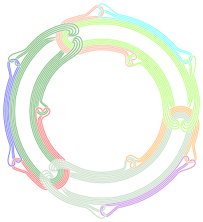
(b) 2nd order Brunnian rings

Figure 4. Links

11. Conclusion

The purpose of this paper is to introduce and formulate the basic principles of higher structures occuring in science and nature in general and in mathematics in particular. This suggests extensions of known mathematical theory, but also leads to situations where new mathematical theory has to be developed. This program of Hyperstructures may go in many directions and we just consider this paper as an eye opener of where to go in the future.

Acknowledgements

I would like to thank P. Cohen, D. Sullivan and V. Voevodsky for interesting discussions at various stages of the development of the mathematical aspects of the hyperstructure concept.

I would also like to thank M. Thaule for his kind technical assistance in preparing the manuscript. I would like to thank A. Stacey for producing Figure 4.

Notes on the contributor

Nils A. Baas was born in Arendal, Norway, 1946. He was educated at the University of Oslo where he got his final degree in 1969. Later on he studied in Aarhus and Manchester. He was a Visiting Assistant Professor at U. Va. Charlottesville, USA in 1971–1972. Member of IAS, Princeton in 1972–1975 and IHES, Paris in 1975. Associate Professor at the University of Trondheim, Norway in 1975–1977 and since 1977, Professor at the same university till date. He conducted research visits to Berkeley in 1982–1983 and 1989–1990; Los Alamos in 1996; Cambridge, UK in 1997, Aarhus in 2001 and 2004. He was Member IAS, Princeton 2007, 2010, 2013 and 2016. His research interests include: algebraic topology, higher categories and hyperstructures and topological data analysis.

References

- Ayala et al. [2015] D. Ayala, J. Francis, and N. Rozenblyum. Factorization homology I: higher categories. Preprint arXiv:1504.04007, 2015.
- Baas [1994] N.A. Baas. Hyper-structures as a tool in nanotechnology. Nanobiology, 3(1):49–60, 1994.
- Baas [1996] N.A. Baas. Higher order cognitive structures and processes. In Toward a Science of Consciousness, pages 633–648. MIT Press, Cambridge, 1996.
- Baas [2006] N.A. Baas. Hyperstructures as abstract matter. Adv. Complex Syst., 9(3):157–182, 2006.
- Baas [2009a] N.A. Baas. New structures in complex systems. Eur. Phys. J. Special Topics, 178:25–44, 2009a.
- Baas [2009b] N.A. Baas. Hyperstructures, topology and datasets. Axiomathes, 19(3):281–295, 2009b.
- Baas [2013a] N.A. Baas. New states of matter suggested by new topological structures. Int. J. Gen. Syst., 42(2):137–169, 2013a. arXiv:1012.2698
- Baas [2013b] N.A. Baas. On structure and organization: an organizing principle. Int. J. Gen. Syst., 42(2):170–196, 2013b. arXiv:1201.6228
- Baas [2015] N.A. Baas. Higher order architecture of collections of objects. Int. J. Gen. Syst., 44(1):55–75, 2015. arXiv:1409.0344
- Baas [2016] N.A. Baas. On higher structures. Int. J. Gen. Syst., 45(6):747–762, 2016. arXiv:1509.00403
- Baas [2017] N.A. Baas. On the concept of space in neuroscience. Current Opinion in Systems Biology, 1:32–37, 2017.
- Baas [2018a] N.A. Baas. On the philosophy of higher structures. Int. J. Gen. Syst., in press. https://doi.org/10.1080/03081079.2019.1584894 arXiv:1805.11943
- Baas [2018b] N.A. Baas. Topology and Higher Concurrencies. Preprint arXiv:1805.06760, 2018.
- Baas et al. [2004] N.A. Baas, A.C. Ehresmann, and J.-P. Vanbremeersch. Hyperstructures and memory evolutive systems. Int. J. Gen. Syst., 33(5):553–568, 2004.
- Baas et al. [2014] N.A. Baas, D.V. Fedorov, A.S. Jensen, K. Riisager, A.G. Volosniev, and N.T. Zinner. Higher-order brunnian structures and possible physical realizations. Physics of Atomic Nuclei, 77(3):336–343, 2014.
- Baas and Seeman [2012] N.A. Baas and N.C. Seeman. On the chemical synthesis of new topological structures. J. Math. Chem., 50(1):220–232, 2012.
- Baas et al. [2015] N.A. Baas, N.C. Seeman, and A. Stacey. Synthesising topological links. J. Math. Chem., 53(1):183–199, 2015.
- Baas and Stacey [2016] N.A. Baas and A. Stacey. Investigations of Higher Order Links. Preprint arXiv:1602.06450, 2016.
- Ginot [2015] G. Ginot. Notes on factorization algebras, factorization homology and applications. In Mathematical aspects of quantum field theories, Math. Phys. Stud., edited by D. Calaque and T. Strobl, pages 429–552. Springer, Cham, 2015.
- Haugseng [2018] R. Haugseng. Iterated spans and classical topological field theories. Math. Z, 289(3-4): 1427–1488, 2018.
- Mac Lane [1998] S. Mac Lane. Homology, volume 114 of Die Grundlehren der mathematischen Wissenschaften. Springer-Verlag, Berlin-New York, 1967.
- Mac Lane and Moerdijk [1994] S. Mac Lane and I. Moerdijk. Sheaves in geometry and logic, Universitext. Springer-Verlag, New York, corrected reprint of the 1992 edition, 1994.
- Lurie [2009a] J. Lurie. On the classification of topological field theories. In Current developments in mathematics, 2008, edited by D. Jerison, B. Mazur, T. Mrowawka, W. Schmid, R. Stanley and S.-T. Yau, pages 129–280. International Press, Somerville, MA, 2009a.
- Lurie [2009b] J. Lurie. Higher topos theory, volume 170 of Annals of Mathematics Studies. Princeton University Press, Princeton, NJ, 2009b.
- Leinster [2004] T. Leinster. Higher Operads, Higher Categories, volume 298 of London Mathematical Society Lecture Note Series. Cambridge University Press, Cambridge, 2004.