Coincidence landscapes for polarized bosons

Abstract

Passive optical interferometry with single photons injected into some input ports and vacuum into others is enriched by admitting polarization, thereby replacing the scalar electromagnetic description by a vector theory, with the recent triad phase being a celebrated example of this richness. On the other hand, incorporating polarization into interferometry is known to be equivalent to scalar theory if the number of channels is doubled. We show that passive multiphoton $m$-channel interferometry described by SU($m$) transformations is replaced by SU($2m$) interferometry if polarization is included and thus that the multiphoton coincidence landscape, whose domain corresponds to various relative delays between photon arrival times, is fully explained by the now-standard approach of using immanants to compute coincidence sampling probabilities. Consequently, we show that the triad phase is manifested simply as SU(6) interferometry with three input photons, with one photon in each of three different input ports. Our analysis incorporates passive polarization multichannel interferometry into the existing scalar-field approach to computing multiphoton coincidence probabilities in interferometry and demystifies the triad phase.

I Introduction

Two-photon interference has been studied extensively since the celebrated 1987 Hong-Ou-Mandel (HOM) experiment Hong et al. (1987). Also known as the HOM dip, this phenomenon is manifested as two identical photons whose relative arrival times are controlled by a time-delay mechanism, thereby controlling their relative distinguishability. The photons arrive at a balanced (50:50) beam splitter with each entering a different input port. Light from the two output ports is directed to two photon counters and the resultant signal is multiplied. In the quantum description, the HOM dip corresponds to a null coincidence for zero relative time delay: the quantum mechanical description forbids each detector to see a photon when they are indistinguishable. For long delays relative to the duration of the photonic wave packet, each photon has a 50% chance of being reflected or transmitted so the coincidence probably is one-half. The HOM phenomenon provides a vital tool for characterizing single-photon sources Santori et al. (2002) and for preparing and detecting entangled photonic qubits Knill et al. (2001); Marcikic et al. (2003); Su et al. (2017).

This destructive interference between two photons can be generalized to the case of $n$ photons Campos (2000); Mährlein et al. (2015); Lim and Beige (2005). For three-photon interference, each photon is injected into different input ports, and the interest is in the coincidence of three-photon interference with one photon in separate output ports. The coincidence rate appears as a landscape tuned by two variables, with the time delays of two photons relative to a third, used as reference. Not only do we obtain the destructive dip, but we also obtain a constructive peak in the three-photon landscape Tan et al. (2013); de Guise et al. (2014); Tillmann et al. (2015).

A systematic generalization from the two-photon to high-order coincidence dips or peaks arises from treating such scattering transformations as elements of a unitary group. In this scheme, the lossless beam splitter is characterized as a U(2) transformation [SU(2) with a global phase] for the photon’s states Yurke et al. (1986); Campos et al. (1989). Using the four-port beam splitter as building blocks, an arbitrary U($m$) interferometer with $m$ input ports and $m$ output ports is achieved as a sequence of beam splitters and phase shifters de Guise et al. (2018); Clements et al. (2016); Reck et al. (1994); Rowe et al. (1999). Below we omit the global phase as it has no effect on the coincidence rate, in which case we write SU($m$) rather than U($m$).

In this paper, we consider the U($m$) matrix to be fixed and focus on the parameters that come from the injected bosons, i.e., the time delays or the polarization spectrum. The analysis of coincidence landscapes in our work is thus different from the landscapes considered in Mährlein et al. (2015), where these authors have adjustable parameters for the scattering interferometer and their injected photons are indistinguishable.

There are several equivalent approaches to computing the coincidence rates when there are $n$ photons entering an otherwise arbitrary SU($m$) interferometer. Some approaches rely heavily on permanents Shchesnovich (2015); Tichy (2015); Tamma and Laibacher (2015); they have the advantage of familiarity and a well-known algorithm, namely, Ryser’s algorithm Ryser (1963), to evaluate the permanent of any matrix.

An alternative is to recognize that additional (even considerable) insight into many-body problems is often obtained by the use of symmetric-group methods. Using Schur-Weyl duality between the symmetric group S_n of $n$ objects and the unitary group U($m$) yields an immanant-based formalism that makes coincidence landscapes amenable to interpretations based on permutational symmetries of photons described by S_n Tan et al. (2013); de Guise et al. (2014); Tillmann et al. (2015); Khalid et al. (2018). Immanants naturally account for the partial distinguishability of photons, and the idea of “immanon” Tichy and Mølmer (2017) has been introduced in an attempt to capture the feature. Although the use of Schur-Weyl duality brings elegance to this alternative approach, immanants are not so well known and good algorithms to compute them are not common, even if a close connection (going back to Kostan Kostan (1995)) between immanants and group functions can be exploited Bürgisser (2000); de Guise et al. (2016).

Despite this paucity of algorithms, the problem of reducing a representation of $S_{n}$ is well studied and can be transformed to an eigenvalue problem using class operators Chen et al. (2002). Most important, this reduction is independent of the details of the scattering network, so that the transformation effecting the block diagonalization can be precomputed with prior knowledge only of the input and output configurations of the system Khalid et al. (2018). An example of this feature can be found in Eq. (85) of Appendix B.

Here we generalize previous results Tan et al. (2013); de Guise et al. (2014); Tillmann et al. (2015); Khalid et al. (2018) to accommodate interference of polarized photons. The case of more than one photon in an input or output port means that possible representations of S_n are a subset of all the possible irreducible representations (irreps) and is treated in Khalid et al. (2018). We show in particular that the tools based on the symmetric group and developed for the analysis of photons which are temporally partially distinguishable can be extended to include partial distinguishability in polarization; in other words, all the insights provided by the use of immanants remain, provided we consider both polarization and temporal degrees of freedom (labeled by $\bm{\theta}$ and $\bm{\tau}$, respectively) in the distinguishability features of the photons.

We give, in Eq. (79) of Appendix B, an expression for the rate

$$C(\bm{\theta};\bm{\tau}),$$ (1)

which agrees with the result of Tichy (2015), but can be usefully converted to an expression

$$C(\bm{\theta};\bm{\tau})=\sum_{i,j}u_{i}^{*}R_{ij}(\bm{\theta};\bm{\tau})u_{j},$$ (2)

where further block diagonalization of $R_{ij}$ will produce a rate (using the standard tools of the symmetric group) in terms of moduli squared of sums of immanants written as combinations of $u_{i}$’s.

Typically multiphoton interference is treated as a scalar field theory: polarization is ignored. Ignoring polarization is not detrimental for studying multiphoton interferometry as polarization can rather trivially be converted to a path degree of freedom. Polarization is included in $m$-channel interferometry by combining a U(2) transformation with a U($m$) transformation, resulting in U($2m$) irreps using the subchain

$$\text{U}(2m)\supset\text{U}(m)\times\text{U}(2)$$ (3)

transformation and the dual pair of U(2) and U($m$) when the same U(2) polarization transformation acts on all spatial modes Rowe et al. (1999). Dhand and Goyal decomposed arbitrary unitary transformations for photonic states in terms of spatial and internal modes Dhand and Goyal (2015). Manipulating internal and external degrees of freedom in multiphoton interference has recently attracted significant attention Menssen et al. (2017); Agne et al. (2017).

Despite a mathematical equivalence between polarization and path degrees of freedom, some confusion has arisen about the sufficiency of mutual photon distinguishability in explaining the features of coincidence rates. As a specific example, Menssen et al. used a symmetric three-port interferometer, known as a tritter Jex et al. (1995); Żukowski et al. (1997), to implement two- and three-photon interference with polarized photons Menssen et al. (2017). They then claim that “the distinguishability between pairs of photons is not sufficient to fully describe the photons’ behavior in a scattering process, but that a collective phase, the triad phase, plays a role” Menssen et al. (2017). Agne et al. Agne et al. (2017) showed this collective phase in entangled-photon experiments. A chief goal of our work is to show that polarization degrees of freedom, independent for each physical mode, are trivially absorbed into an SU($2m$) transformation.

In Sec. II, we show how to construct the special unitary network with doubling of ports when polarization is taken into consideration. Then we calculate the coincidence rate for polarization-sensitive and -insensitive events in our framework in Sec. III. In Sec. IV, we focus on the case when $m=3$ and clarify the triad phase in our framework.

II From SU($m$) to SU($2m$)

In this section, we give the general framework to deal with the polarized multiphoton interference problem in a polarization-sensitive scattering network. We generalize a discussion in Rowe et al. (1999) to easily incorporate polarization into scalar-field interferometry by converting polarization to path. If the polarization transformations on each spatial modes are identical, “one simply extends the U($n$) group to U($n$)$\times$U(2) and to include combinations of polarizers and beam splitters, for example, one extends to $\text{U}(2n)\supset\text{U}(n)\times\text{U}(2)$ Rowe et al. (1999). ” Rowe et al. (1999). Here we consider the polarization transformations being distinct on all the spatial modes.

First, notice that we can construct a U(2) transformation matrix for the polarization. For a photon injecting in the $i$th port of an $m$-channel polarization-sensitive interferometer, the input state is

$$\Ket{\Psi_{i}}=\sum_{\alpha=1}^{2}c^{(i)}_{\alpha}A^{\dagger}_{i\alpha}(\tau_{i})\Ket{0},$$ (4)

and

$$A^{\dagger}_{i\alpha}(\tau_{i}):=\int\text{d}\omega\phi_{i}(\omega)\text{e}^{-\text{i}\tau_{i}\omega}a_{i\alpha}^{\dagger}(\omega)\,.$$ (5)

Here $\tau_{i}$ is the time delay of the $i$th photon; $a^{\dagger}_{i\alpha}$ is the creation operator for the photon mode of the $i$th spatial port and $\alpha$th polarization. Thus, $\alpha=1$ and $\alpha=2$ represent two orthogonal polarizations, e.g., horizontal and vertical polarizations or left-handed and right-handed polarizations.

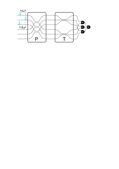
Figure 1: Decomposition of interference network and setup for the detectors.

Without loss of generality, we use $\alpha=1$ to represent horizontal polarization and $\alpha=2$ to represent vertical polarization; $|\phi(\omega)|^{2}$ is the frequency profile in the frequency domain satisfying

$$\int\text{d}\omega|\phi(\omega)|^{2}=1.$$ (6)

Coefficients $\{c_{\alpha}^{(i)}\in\mathbb{C}\}$ satisfy

$$\sum_{\alpha=1}^{2}|c_{\alpha}^{(i)}|^{2}=1.$$ (7)

These coefficients $\{c_{\alpha}^{(i)}\}$ describe a U(2) transformation $P^{(i)}$ on the $i$th photon’s polarization as

$$P^{(i)}:=\begin{pmatrix}c_{1}^{(i)}&-\text{e}^{\text{i}\psi}c_{2}^{*(i)}\\ c_{2}^{(i)}&\text{e}^{\text{i}\psi}c_{1}^{*(i)}\end{pmatrix},$$ (8)

where $\psi$ is an overall phase.

For $m$ spatial modes, the polarization transformation is

$$P:=\oplus_{i=1}^{m}P^{(i)}.$$ (9)

We model the scattering network $T$ to be polarization sensitive by factoring the net effect of the network into individual polarization transformation for each spatial mode followed by a transformation mixing modes for the same polarization, which takes the form

$$T:=\tilde{T}^{(1)}\oplus\tilde{T}^{(2)},$$ (10)

where $\tilde{T}^{(\alpha)}$ is the mode transformation acting on photons with polarization $\alpha$ alone. Here we assume $\tilde{T}^{(1)}=\tilde{T}^{(2)}$ in the respective polarization subspaces.

For convenience, we specify the basis order by using one single subscript to replace the spatial and polarization subscripts: $a_{k}^{\dagger}:=a_{i\alpha}^{\dagger}$, with

$$a^{\dagger}_{k}=a^{\dagger}_{i1},\;k=i=1,\dots,m$$ (11)

and

$$a^{\dagger}_{k}=a^{\dagger}_{i2},\;k=i+m,i=1,\dots,m.$$ (12)

In this subscript notation, the first $k$ labels up to $k=m$ refer to horizontally polarized photons, while the next $k$ labels from $m+1$ to $2m$ refer to vertically polarized photons. For example, when $m=3,n=2$, $a^{\dagger}_{12}$ is replaced by $a^{\dagger}_{4}$, which is the creation operator of horizontally polarized photon in the first spatial mode.

Thus, by ignoring the phase shift in Eq. (8) as it will not affect the result of coincidence, our original SU($m$) scattering network spanned by $m$ space-mode states is expanded to an $\text{SU}(2m)$ transformation

$$U=TP$$ (13)

spanned by $2m$ orthogonal space-and-polarization-mode states (see Fig. 1 as an example when $m=3$) so that photons scatter according to

$$a_{j}^{\dagger}\mapsto Ua_{j}^{\dagger}U^{\dagger}=\sum_{i=1}^{2m}a_{i}^{\dagger}U_{ij},$$ (14)

where $a^{\dagger}_{i}$ is the creation operator for the photon in the $i$th mode.

Notice that the first index of $U$ represents output and the second index represents input: a photon in input mode $j$ is scattered to a linear combination of photons existing in output mode $i$. The transformation of the creation operators is verified from the photon state’s transformation,

$$U\ket{1_{j}}= Ua_{j}^{\dagger}\ket{0}=Ua_{j}^{\dagger}U^{\dagger}U\ket{0}=Ua_{j}^{\dagger}U^{\dagger}\ket{0}$$ (15)

$$= \sum_{i}\ket{1_{i}}\bra{1_{i}}U\ket{1_{j}}=\sum_{i}a_{i}^{\dagger}U_{ij}\ket{0},$$ (16)

where $\ket{1_{i}}$ is the state that one photon is in the $i$th mode. Comparing the last equations in Eqs. (15) and (16), we obtain the creation-operator transformation (14). Using Fig. 1, we confirm the factorization $U=TP$ of Eq. (13).

For $m=3$ modes, the explicit matrix representation of the SU(6) transformation $T$ can be

$$T=\begin{pmatrix}\tilde{T}&0\\ 0&\tilde{T}\end{pmatrix}$$ (17)

with $\tilde{T}$ the original 3$\times$3 transformation matrix. By writing the independent polarization transformations $P^{(1)},P^{(2)},P^{(3)}$ as per Eq. (8), we construct the polarization transformation

$$P =P^{(1)}\oplus P^{(2)}\oplus P^{(3)}$$ (18)

$$=\begin{pmatrix}P^{(1)}_{11}&0&0&P^{(1)}_{12}&0&0\\ 0&P^{(2)}_{11}&0&0&P^{(2)}_{12}&0\\ 0&0&P^{(3)}_{11}&0&0&P^{(3)}_{12}\\ P^{(1)}_{21}&0&0&P^{(1)}_{22}&0&0\\ 0&P^{(2)}_{21}&0&0&P^{(2)}_{22}&0\\ 0&0&P^{(3)}_{21}&0&0&P^{(3)}_{22}\\ \end{pmatrix}.$$ (19)

Thus, the total SU(6) transformation is

$$U(\bm{\theta})=TP(\bm{\theta})\\ =\begin{pmatrix}P^{(1)}_{11}\tilde{T}_{11}&P^{(2)}_{11}\tilde{T}_{12}&P^{(3)}_{11}\tilde{T}_{13}&P^{(1)}_{12}\tilde{T}_{11}&P^{(2)}_{12}\tilde{T}_{12}&P^{(3)}_{12}\tilde{T}_{13}\\ P^{(1)}_{11}\tilde{T}_{21}&P^{(2)}_{11}\tilde{T}_{22}&P^{(3)}_{11}\tilde{T}_{23}&P^{(1)}_{12}\tilde{T}_{21}&P^{(2)}_{12}\tilde{T}_{22}&P^{(3)}_{12}\tilde{T}_{23}\\ P^{(1)}_{11}\tilde{T}_{31}&P^{(2)}_{11}\tilde{T}_{32}&P^{(3)}_{11}\tilde{T}_{33}&P^{(1)}_{12}\tilde{T}_{31}&P^{(2)}_{12}\tilde{T}_{32}&P^{(3)}_{12}\tilde{T}_{33}\\ P^{(1)}_{21}\tilde{T}_{11}&P^{(2)}_{21}\tilde{T}_{12}&P^{(3)}_{21}\tilde{T}_{13}&P^{(1)}_{22}\tilde{T}_{11}&P^{(2)}_{22}\tilde{T}_{12}&P^{(3)}_{22}\tilde{T}_{13}\\ P^{(1)}_{21}\tilde{T}_{21}&P^{(2)}_{21}\tilde{T}_{22}&P^{(3)}_{21}\tilde{T}_{23}&P^{(1)}_{22}\tilde{T}_{21}&P^{(2)}_{22}\tilde{T}_{22}&P^{(3)}_{22}\tilde{T}_{23}\\ P^{(1)}_{21}\tilde{T}_{31}&P^{(2)}_{21}\tilde{T}_{32}&P^{(3)}_{21}\tilde{T}_{33}&P^{(1)}_{22}\tilde{T}_{31}&P^{(2)}_{22}\tilde{T}_{32}&P^{(3)}_{22}\tilde{T}_{33}\end{pmatrix},$$ (20)

which clearly transforms the SU(3) description into a SU(6) description.

The cost of doubling the dimension of the problem is that the $2m\times 2m$ scattering matrix $U$ is no longer completely specified by the original $m\times m$ matrix $T$, but now depends on the parameters of the polarization transformations $P^{(k)}$. We denote by $\bm{\theta}$ the collection of polarization parameters needed to specify the various $P^{(k)}$, and hence the argument for $U(\bm{\theta})$ and $P(\bm{\theta})$. The benefit of this doubling is that all the tools available for the discussion of unpolarized photons can simply be imported ipso facto to the problem that includes polarization.

We conclude this section with a discussion of a special case, already hinted at earlier. If the polarization transformations $P^{(i)}$ of Eq. (9) are all identical, then the transformations $T$ and $P$ that define $U$ in Eq. (13) actually commute, i.e.,

$$U=TP=PT.$$ (21)

The transformation SU($2m$) then factors into $\text{SU}(m)\otimes\text{SU}(2)$, and by combining with the overall phase shift, we are back to the Rowe et al. case Rowe et al. (1999).

This factorization of Eq. (21) is of particular interest when photons are fully indistinguishable. In this case, the representation of SU($2m$) must be “fully symmetric”, or transform by an irrep of the type $(n,0,\dots)$ of SU($2m$). As explained in Rowe et al. (1999), this constrains the possible irreps of $\text{SU}(m)\otimes\text{SU}(2)$: the SU(2) and SU($m$) representations must be associated with identical Young diagrams Hagen and Macfarlane (1965), so that by preparing $n$ photons in a definite state of polarization [i.e., a definite SU(2) irrep] these photons are simultaneously prepared in SU($m$) irreps with nontrivial spatial permutation symmetries. This is the optical analog of combining spin and spatial wave functions of specified permutation symmetry to construct a fully symmetric wave function for $n$ bosons.

III Coincidence Rate

In this section, we give the coincidence rate for polarized multiphoton interference, augmenting an earlier discussion where the polarization was not explicitly discussed in the immanant-based formalism Tan et al. (2013); de Guise et al. (2014); Tillmann et al. (2015); Khalid et al. (2018). Here we give the polarization-insensitive and -sensitive detection cases using the immanant-based formalism.

For polarization-sensitive detection, we first define the $n$-dimensional input configuration vector $\bm{v}$, whose entry $v_{i}\in\Set{1,2,\dots,2m}$ indicates which input mode the $i$th photon occupies. For convenience of description, we also use a $2m$-dimensional input mode-occupation vector $\bm{\xi}^{\bm{v}}$ to represent the same input state, whose entry

$$\xi^{\bm{v}}_{i}\in\Set{0,1,\dots,n}$$ (22)

tells how many photons are in the $i$th mode, and

$$\sum_{i=1}^{2m}\xi^{\bm{v}}_{i}=n.$$ (23)

Similarly, we define an $n$-dimensional output configuration vector $\bm{\eta}$ and a $2m$-dimensional output mode-occupation vector $\bm{\xi}^{\bm{\eta}}$, with

$$\eta_{i}\in\Set{1,2,\dots,2m},\;\xi^{\bm{\eta}}_{i}\in\Set{0,1,\dots,n},$$ (24)

and

$$\sum_{i=1}^{2m}\xi^{\bm{\eta}}_{i}=n.$$ (25)

For polarization-insensitive detectors, we also define another output configuration $\bm{\mu}$, called regular output configuration, with entry

$$\mu_{i}\in\Set{1,2,\dots,m}.$$ (26)

Now we inject $n$ photons into the SU($2m$) interferometer $U$ to obtain the input state

$$\Ket{\Psi_{\text{in}}}:=\mathsf{N}\prod_{i=1}^{n}A_{v_{i}}^{\dagger}(\tau_{i})\Ket{0}$$ (27)

where

$$\mathsf{N}=\frac{1}{\sqrt{\xi^{\bm{v}}_{1}!\,\xi^{\bm{v}}_{2}!\,\dots\xi^{\bm{v}}_{2m}!}}$$ (28)

is a normalization constant and

$$A_{v_{i}}^{\dagger}(\tau_{i}):=\int\text{d}\omega\phi_{v_{i}}(\omega)\text{e}^{-\text{i}\tau_{i}\omega}a_{v_{i}}^{\dagger}(\omega).$$ (29)

The resultant output state is

$$\Ket{\Psi_{\text{out}}} :=U\Ket{\Psi_{\text{in}}}$$ (30)

$$=\mathsf{N}\prod_{i=1}^{n}\int\text{d}\omega\phi_{v_{i}}(\omega)\text{e}^{-\text{i}\tau_{i}\omega}\sum_{j=1}^{2m}U_{jv_{i}}a_{j}^{\dagger}(\omega)\Ket{0}.$$ (31)

We next need to specify the measurements for different kinds of detectors. We divide them into two categories of detectors for polarized single photons: ideal polarization-sensitive detectors and practical polarization-insensitive detectors.

For the polarization-sensitive detectors, one polarization-sensitive detector is equivalent to the combination of a polarizing beam splitter and two polarization-insensitive detectors. Our separation of the polarization from the spatial mode, which results in the expansion from SU($m$) to SU($2m$), has played the role of polarizing beam splitters. Then the detection operator for this specific output configuration $\bm{\eta}$ is

$$M_{\bm{\eta}}:=\frac{1}{\xi^{\bm{\eta}}_{1}!\,\xi^{\bm{\eta}}_{2}!\,\dots\xi^{\bm{\eta}}_{2m}!}\int\text{d}\bm{\omega}\prod_{i=1}^{n}a_{\eta_{i}}^{\dagger}(\omega_{i})\Ket{0}\Bra{0}a_{\eta_{i}}(\omega_{i}).$$ (32)

However, in most boson sampling or multiphoton interference experiments Broome et al. (2013); Spring et al. (2013); Tillmann et al. (2013); Crespi et al. (2013); Tillmann et al. (2015); Wang et al. (2017); Menssen et al. (2017), one usually uses the polarization-insensitive detectors for the single-photon detection, such as avalanche photodiodes detectors (APDs), especially single-photon avalanche diode detectors (SPADs). We deal with the frequency-insensitive detector by summing over the polarizations corresponding to the same regular output configuration $\bm{\mu}$. This set of configurations is

$$\mathfrak{S}_{\bm{\mu}}:=\Set{\bm{\eta}\mid\forall i\in\Set{1,2,\dots,n},\eta_{i}\in\Set{\mu_{i},\mu_{i}+m}}$$ (33)

and

$$|\mathfrak{S}_{\bm{\mu}}|=2^{n}.$$ (34)

For example, for a $2\times 2$ spatial scattering interferometer such as a beam splitter, injecting two photons from input ports 1 and 2, the input configuration is $\bm{v}=(1,2)$. Then to detect the coincidence of the photons’ output from spatial ports 1 and 2, respectively, the regular output configuration $\bm{\mu}=(1,2)$, and

$$\mathfrak{S}_{\bm{\mu}}=\{(1,2),(1,4),(3,2),(3,4)\},$$ (35)

which contains all possible polarizations for the photons’ output to spatial ports 1 and 2. Thus, detection for the regular output configuration $\bm{\mu}$ is

$$M_{\bm{\mu}}:=\sum_{\bm{\eta}\in\mathfrak{S}_{\bm{\mu}}}M_{\bm{\eta}}.$$ (36)

We have now formulated how our original problem becomes the problem that $n$ identically polarized (or horizontally polarized) photons injected into a $2m$-channel interferometer $U$. A key point for later discussion is that, in order to proceed, one must select an $n\times n$ submatrix $\tilde{U}(\bm{\theta})$ of $U(\bm{\theta})$ and this submatrix, which is specified by the input and output configurations, and also depends on $\bm{\theta}$.

As an example, consider the $3\times 3$ tritter matrix $T$ given in Menssen et al. (2017). If the input state contains three photons with horizontal polarizations, and the output state is given by the first two photons with horizontal and the last with vertical polarization, the $6\times 6$ matrix $U(\bm{\theta})$ for the polarized network collapses to a $3\times 3$ submatrix $\tilde{U}$ given by

$$\tilde{U}(\bm{\theta})=\frac{1}{\sqrt{3}}\begin{pmatrix}P^{(1)}_{11}(\bm{\theta}_{1})&P^{(2)}_{11}(\bm{\theta}_{2})&P^{(3)}_{11}(\bm{\theta}_{3})\\ P^{(1)}_{11}(\bm{\theta}_{1})&\zeta^{2}P^{(2)}_{11}(\bm{\theta}_{2})&\zeta P^{(3)}_{11}(\bm{\theta}_{3})\\ P^{(1)}_{21}(\bm{\theta}_{1})&\zeta P^{(2)}_{21}(\bm{\theta}_{2})&\zeta^{2}P^{(3)}_{21}(\bm{\theta}_{3})\\ \end{pmatrix}$$ (37)

with $\zeta=\text{e}^{\text{i}\frac{2\pi}{3}}$. Consequently, experiments where the polarization parameters $\bm{\theta}$ are changed are equivalent to experiments where the scattering submatrix $\tilde{U}(\bm{\theta})$ is changed. Coincidence rates are therefore expected to depend on $\bm{\theta}$, even if the matrix $\tilde{T}$ that scatters the spatial modes is kept constant from one experiment to the next, and even if the input and output states remain the same as we vary $\bm{\theta}$.

For detection modeled by Eq. (32), the coincidence rate for the polarization-sensitive detectors for the output configuration $\bm{\eta}$ is Khalid et al. (2018)

$$C_{\bm{\eta}}(\bm{\theta};\bm{\tau}):=\bm{u}^{\dagger}_{\bm{\eta}}(\bm{\theta})R({\bm{\tau}})\bm{u}_{\bm{\eta}}(\bm{\theta})$$ (38)

where $\bm{u}_{\bm{\eta}}(\bm{\theta})$ is an

$$N_{\bm{\eta}}=\frac{n!}{\xi^{\bm{\eta}}_{1}!\,\xi^{\bm{\eta}}_{2}!\,\dots\xi^{\bm{\eta}}_{2m}!}$$ (39)

dimensional vector, that contains all the information about the submatrix of our SU($2m$) scattering matrix. The vector entries are

$$\left(\bm{u}_{\bm{\eta}}(\bm{\theta})\right)_{k}=\prod_{i=1}^{n}U(\bm{\theta})_{\bar{\eta}^{(k)}_{i}v_{i}},\text{for}\,k=1,2,\dots,N_{\bm{\eta}}$$ (40)

with

$$\bar{\bm{\eta}}^{(k)}\in\set{\bar{\bm{\eta}}}{\bar{\bm{\eta}}=\sigma{\bm{\eta}},\,\sigma\in\text{S}_{n}}.$$ (41)

The action of $\sigma$ on $\bm{\eta}$ sends the $i$th element to the $\sigma(i)$th; for instance, if $\sigma=(123)$, then its action on $(1,2,3)$ yields $(3,1,2)$. $\bar{\eta}^{(k)}$s provide a basis of the representation of the symmetric group S_n.

The rate matrix $R(\bm{\tau})$ is

$$R(\bm{\tau}):=\sum_{\sigma\in S_{n}}\mathsf{B}_{\sigma}(\bm{\tau})\Pi_{\sigma},$$ (42)

where $\Pi_{\sigma}$ is a permutation matrix with elements

$$(\Pi_{\sigma})_{ij}:=\delta(\sigma\bar{\bm{\eta}}^{i},\bar{\bm{\eta}}^{j})=\begin{cases}1&\sigma\bar{\bm{\eta}}^{i}=\bar{\bm{\eta}}^{j},\\ 0&\text{otherwise}.\end{cases}$$ (43)

For the specific case where there are $n$ photons in $n$ distinct output modes, $\Pi_{\sigma}$ is the $n\times n$ regular representation of $\sigma\in\text{S}_{n}$. $\mathsf{B}_{\sigma}$ is the overlap between the input state and the $\sigma$-permuted input state,

$$\mathsf{B}_{\sigma}:=\prod_{i=1}^{n}\beta_{v_{\sigma(i)},v_{i}},$$ (44)

where $\beta_{i,j}$ is the two-photon pairwise distinguishability between the $i$th and $j$th photons.

Definition (44) agrees with the distinguishability matrix obtained in Tichy (2015). Specifically, for the polarization-sensitive case, $\mathsf{B}_{\sigma}$ is only dependent on the time delays $\bm{\tau}$ as $\mathsf{B}_{\sigma}(\bm{\tau})$ because the overlap is only the spectrotemporal overlap,

$$\beta_{ij}(\bm{\tau})=\int\text{d}\omega\phi^{*}_{i}(\omega)\phi_{j}(\omega)\text{e}^{\text{i}\omega(\tau_{i}-\tau_{j})}.$$ (45)

Having given the coincidence rate for the polarization-sensitive detectors in Eq. (38), we now give the coincidence rate for the polarization-insensitive detectors. With the detection operator defined in Eq. (36), the coincidence is easily obtained as the sum of the coincidence rate of all the configurations in $\mathfrak{S}_{\bm{\mu}}$, namely,

$$C_{\bm{\mu}}(\bm{\theta};\bm{\tau}):=\sum_{\bm{\eta}\in\mathfrak{S}_{\bm{\mu}}}C_{\bm{\eta}}(\bm{\theta};\bm{\tau})=\bm{u}^{\dagger}_{\bm{\mu}}R(\bm{\theta};{\bm{\tau}})\bm{u}_{\bm{\mu}}$$ (46)

The derivation for the last equation is given in Appendix A.

Our key observation is that the effects of the polarization can be incorporated into a rate matrix so

$$R(\bm{\tau})\to R(\bm{\theta};\bm{\tau})$$ (47)

while making the vectors $\bm{u}_{\eta}(\theta)\to\bm{u}_{\mu}$ independent of the polarization parameters without affecting the permutation matrices $\Pi_{\sigma}$. Specifically, the resulting coincidence rate is the same as $n$ photons in the original SU($m$) scattering interferometer $\tilde{T}$, except that the polarizations are absorbed in the pairwise terms $\beta_{ij}(\bm{\tau})\to\beta_{ij}(\bm{\theta};\bm{\tau})$ as

$$\beta_{ij}(\bm{\theta};\bm{\tau})= \sum_{k=1}^{2}P^{*(i)}_{k1}(\bm{\theta})P^{(j)}_{k1}(\bm{\theta})$$

$$\times\int\text{d}\omega\phi^{*}_{i}(\omega)\phi_{j}(\omega)\text{e}^{\text{i}\omega(\tau_{i}-\tau_{j})}.$$ (48)

Substituting it back into Eq. (44) yields that $\mathsf{B}_{\sigma}$, as well as the rate matrix $R$, depend on both time delay $\bm{\tau}$ and polarization $\bm{\theta}$.

As the permutation matrices $\{\Pi_{\sigma}\}$ are unaffected by including polarization parameters, both rate matrices in Eqs. (38) and (46) are further reduced by simultaneously diagonalizing class operators of symmetry group S_n Chen et al. (2002). From this reduction procedure, we obtain a basis transformation $V$ to transform the basis to the basis with permutational symmetry, which is a linear combination of immanants.

The general formulas of immanant for a matrix $W$ are

$$\text{Imm}_{\lambda}(W):=\sum_{\sigma\in S_{n}}\chi_{\lambda}(\sigma)\prod_{i=1}^{n}W_{i\sigma(i)},$$ (49)

where $\lambda$ is a partition of $n$ and represents an irreducible representation (irrep) of S_n; $\chi_{\lambda}$ is the character of S_n in $\lambda$ irrep. Thus, Eq. (46) is further written as

$$C_{\bm{\mu}}(\bm{\theta};\bm{\tau})=(V\bm{u})^{\dagger}\left(VR(\bm{\theta};\bm{\tau})V^{\dagger}\right)(V\bm{u}).$$ (50)

By writing the coincidence rate in this reduced form, both the interferometer and the photons are treated in their respective irrep subspaces. Thus, the calculation is simplified when photons or interferometers are biased with specific permutational symmetries (see Appendix B).

IV Triad Phase Demystified

In this section, we give the specific example for $m=3$ and the scattering network is polarization-insensitive:

$$\tilde{T}^{(1)}=\tilde{T}^{(2)}=\tilde{T},$$ (51)

and there is no more than one photon in each spatial mode. First we give the triad phase in our framework. Each element of the distinguishability matrix of Tichy (2015); Menssen et al. (2017) is our $\beta$ (see Appendix B).

In our framework, the triad phase is defined as the argument of the product of three inner products of two photons’ states Menssen et al. (2017),

$$\varphi:=\arg\left(\beta_{31}\beta_{12}\beta_{23}\right).$$ (52)

According to Eqs. (44), (45), and (48) for the polarization-sensitive case,

$$\varphi=\arg\left(\mathsf{B}(\bm{\tau})_{(123)}\right)$$ (53)

and, for the polarization-insensitive case,

$$\varphi=\arg\left(\mathsf{B}(\bm{\theta};\bm{\tau})_{(123)}\right).$$ (54)

In both cases, the triad phase is the argument of the states’ overlap of the three-cycle permutation in the rate matrix $R$.

We also notice that there is a constraint for the triad phase to be an independent variable in the three-photon interference: three photons are identical with the same symmetric density profile around the central frequency Menssen et al. (2017). In that case,

$$\operatorname{arg}(\mathsf{B}(\bm{\tau})_{(123)})=0.$$ (55)

Thus, with a symmetric density profile, for the polarization-sensitive detector, the triad phase is identically zero. For the polarization-insensitive detector, the triad phase is simplified so it is only dependent on the polarization. Thus, the triad phase inherits the independence from the polarization parameters $\bm{\theta}$.

Hence, instead of regarding the triad phase as an independent variable to determine multiphoton coincidence, we see that the polarization parameter itself plays a fundamental role in multiphoton interference. We notice that the polarization and the time delays are both tunable parameters to adjust the photons’ distinguishability; the difference is that the submatrix $\tilde{U}$ depends on $\bm{\theta}$, but not on $\bm{\tau}$, so that continuously changing $\bm{\theta}$ amounts to exploring a parametrized family of $3\times 3$ submatrices $\tilde{U}(\bm{\theta})$, which affects the coincidence rates independently from $\bm{\tau}$.

For the polarization-insensitive case, we can mimic the coincidence rate (46) using three identically polarized photons of spectra $\phi_{1}^{\prime}(\omega)$, $\phi_{2}^{\prime}(\omega)$, $\phi_{3}^{\prime}(\omega)$ in the original SU(3) interferometer $\tilde{T}$. Notice here that the spectra $\phi^{\prime}$ is different from $\phi$, and should not have an identical symmetric density profile because otherwise there is no argument in the three-cycle permutations. Then,

$$\mathsf{B}^{\prime}_{\sigma}({\bm{\tau}^{\prime}})=\mathsf{B}_{\sigma}(\bm{\theta};\bm{\tau}),\,\text{for}\,\forall\sigma\in\text{S}_{3}.$$ (56)

The $3!$ complex equations above correspond to $2\times 3!$ real equations. In these $2\times 3!$ equations, the equation where $\sigma=e$ is trivial.

In the remaining equations, the equations for two-cycle and for three-cycle permutations are not independent. Thus, the number of independent equations is reduced to four: two from one complex equation for three-cycle permutation and the rest from the two real equations for two-cycle permutation. In addition to the three parameters in $\bm{\tau}^{\prime}$, another parameter is needed for the four independent equations. The triad phase Menssen et al. (2017) is one such choice. However, here, the photon’s spectra are not identical. The triad phase $\varphi$ will be dependent on $\bm{\tau}^{\prime}$. Thus, we choose one parameter in the photon’s spectra, for instance, the variance of a Gaussian profile. Then these four independent parameters are determined from Eq. (56).

In summary, the triad phase is not a well-defined independent variable in multiphoton interference. The effect of adding a polarization degree of freedom into multiphoton interference is to change the effective SU($2m$) transformation network. For the polarization-insensitive detection events, $\bm{\theta}$ is absorbed into our rate matrix or the two-photon pairwise distinguishability $\beta$; thus changing $\bm{\theta}$ is effectively changing the indistinguishabilities between photons.

V Conclusion

We have described a model for polarized multiphoton interference in a generalized scattering interferometer, in which the detectors are either polarization sensitive or insensitive. In our model, polarization is merged into the transformation network by doubling the ports to realize an SU($2m$) transformation. By changing polarizations, we consequently change the scattering matrix.

Specifically, for polarization-insensitive detectors, the polarization is merged into our rate matrix, then changing the polarization is equivalently changing the photons’ distinguishabilities. We have shown that the two-photon pairwise distinguishabilities, which include the information about the independent parameters $\bm{\tau}$ and $\bm{\theta}$, already suffice to describe the multiphoton interference.

As the permutation matrices $\Pi_{\sigma}$ are not affected by the introduction of the polarization degree of freedom (as shown explicitly for the $3\times 3$ case in Appendix B), block diagonalization of $R(\bm{\theta},\bm{\tau})$ yields the coincidence rate in terms of immanants. In a generalization of previous results, the distinguishability of a photon is not limited to the temporal overlap of pulses but also include the polarization overlap. In the specific case of three polarized photons, this means that, when two photons are indistinguishable in time and in polarization, the rate will contain a sum of moduli squared of the mixed symmetry $\{2,1\}$ immanant and the permanent, with no contribution from the determinant of the rate matrix $R(\bm{\theta},\bm{\tau})$.

As we scale up to $n$ photons, including input and output states which may contain more than one photon, the subset of immanants that can appear is determined by the distinguishability of the input photons and computed using permutational symmetry methods as per Khalid et al. (2018). This extends the usefulness of the symmetric group in multiphoton interferometry to situations including polarization.

VI Acknowledgments

The work of HdG is supported by NSERC of Canada. HdG would like to thank Dylan Spivak for clarifying discussions. BCS acknowledges China’s 1000 Talent Plan and NSFC (Grant No. 11675164) for support. JW thanks Zheng-Da Li and Hui Wang for valuable discussions.

Appendix A Simplification of coincidence rate of polarization-insensitive detection

In this appendix, we derive Eq. (46) in the main context for the coincidence of polarized photons. With proposition 1 in Khalid et al. (2018), for the measurement in Eq. (36) we obtain the coincidence rate as

$$C_{\bm{\mu}}(\bm{\theta};\bm{\tau}):=\sum_{\bm{\eta}\in\mathfrak{S}_{\bm{\mu}}}C_{\bm{\eta}}(\bm{\theta};\bm{\tau})=\sum_{\bm{\eta}\in\mathfrak{S}_{\bm{\mu}}}\bm{u}_{\bm{\eta}}^{\dagger}(\bm{\theta})R(\bm{\tau})\bm{u}_{\bm{\eta}}(\bm{\theta}).$$ (57)

Each entry in $\bm{u}_{\bm{\eta}}$ is a function of the elements in the submatrix of $U$. From Eqs. (13) and (20),

$$U_{ij}=\tilde{T}_{\Gamma(i),\Gamma(j)}P_{\gamma(i),\gamma(j)}^{(\Gamma(j))},$$ (58)

is an explicit element of $U$, where

$$\gamma(i)=\begin{cases}1\,&i\leq m,\\ 2\,&\text{otherwise}.\end{cases}$$ (59)

indicates the polarization. On the other hand,

$$\Gamma(i)=i+m-m\gamma(i)$$ (60)

indicates which photon the state belongs to. Thus, when $v_{i}\leq m$ for all injected photons, and $\bm{\eta}\in\mathfrak{S}_{\bm{\mu}}$, we obtain

$$\gamma(v_{i})=1,\;\Gamma(v_{i})=v_{i},\Gamma(\bm{\eta})=\bm{\mu}.$$ (61)

Thus, each element in $\bm{u_{\mu}}$ is

$$(\bm{u}_{\bm{\eta}})_{k}:=\prod_{i=1}^{n}U_{\bar{\eta}_{i}^{k},v_{i}}(\bm{\theta})=\prod_{i=1}^{n}\tilde{T}_{\bar{\mu}_{i}^{k},v_{i}}P^{(v_{i})}_{\gamma(\bar{\eta}_{i}^{k}),1}(\bm{\theta}).$$ (62)

Then we write the polarization part out from $\bm{u}_{\bm{\eta}}$ as a product of a diagonal matrix $K_{\bm{\eta}}$, with diagonal elements

$$\left[K_{\bm{\eta}}(\bm{\theta})\right]_{kk}=\prod_{i=1}^{n}P^{(v_{i})}_{\gamma(\bar{\eta}_{i}^{k}),1}(\bm{\theta}),\,\text{for}\,k=1,2,\dots,N,$$ (63)

and $\bm{u}$ with elements

$$u_{k}=\prod_{i=1}^{n}\tilde{T}_{\bar{\mu}_{i}^{k},v_{i}}.$$ (64)

We first sum all output configurations with the rate matrix according to

$$\sum_{\bm{\eta}\in\mathfrak{S}_{\mu}}K_{\bm{\eta}}^{\dagger}(\bm{\theta}) R(\bm{\tau})K_{\bm{\eta}}(\bm{\theta})$$

$$= \sum_{\sigma\in S_{n}}\mathsf{B}_{\sigma}(\bm{\tau})\sum_{\bm{\eta}\in\mathfrak{S}_{\mu}}K_{\bm{\eta}}^{\dagger}(\bm{\theta})\Pi_{\sigma}K_{\bm{\eta}}(\bm{\theta}).$$ (65)

The last summation is simplified to

$$\left(\sum_{\bm{\eta}\in\mathfrak{S}_{\mu}}K_{\bm{\eta}}^{\dagger}(\bm{\theta})\Pi_{\sigma}K_{\bm{\eta}}(\bm{\theta})\right)_{pq}$$

$$= \sum_{\bm{\eta}\in\mathfrak{S}_{\mu}}\left[K^{*}_{\bm{\eta}}(\bm{\theta})\right]_{pp}(\Pi_{\sigma})_{pq}\left[K_{\bm{\eta}}(\bm{\theta})\right]_{qq}$$

$$= \sum_{\bm{\eta}\in\mathfrak{S}_{\mu}}\prod_{i=1}^{n}P^{*(v_{i})}_{\gamma(\bar{\eta}_{i}^{p}),1}(\bm{\theta})\delta(\sigma\bar{\bm{\eta}}^{p},\bar{\bm{\eta}}^{q})\prod_{j=1}^{n}P^{(v_{j})}_{\gamma(\bar{\eta}_{j}^{q}),1}(\bm{\theta})$$

$$= \begin{cases}\sum_{\bm{\eta}\in\mathfrak{S}_{\mu}}\prod_{i=1}^{n}P^{*(v_{\sigma(i)})}_{\gamma(\bar{\eta}_{i}^{p}),1}(\bm{\theta})P^{(v_{i})}_{\gamma(\bar{\eta}_{i}^{p}),1}(\bm{\theta}),&\sigma\bar{\bm{\eta}}^{p}=\bar{\bm{\eta}}^{q},\\ 0,&\text{otherwise}.\end{cases}$$ (66)

And,

$$\sum_{\bm{\eta}\in\mathfrak{S}_{\mu}}\prod_{i=1}^{n}P^{*(v_{\sigma(i)})}_{\gamma(\bar{\eta}_{i}^{p}),1}(\bm{\theta})P^{(v_{i})}_{\gamma(\bar{\eta}_{i}^{p}),1}(\bm{\theta})$$

$$=\prod_{i=1}^{n}\left[P_{11}^{*(v_{\sigma(i)})}(\bm{\theta})P_{11}^{(v_{i})}(\bm{\theta})+P_{21}^{*(v_{\sigma(i)})}(\bm{\theta})P_{21}^{(v_{i})}(\bm{\theta})\right].$$ (67)

Thus, together with Eqs. (64), (65), (66), and (67), we obtain the coincidence rate,

$$C_{\bm{\mu}}(\bm{\tau})=\bm{u}^{\dagger}R(\bm{\theta};\bm{\tau})\bm{u},$$ (68)

with

$$R(\bm{\theta};\bm{\tau}):=\sum_{\sigma\in S_{n}}\mathsf{B}_{\sigma}(\bm{\theta};\bm{\tau})\Pi_{\sigma},$$ (69)

and

$$\mathsf{B}_{\sigma}(\bm{\theta};\bm{\tau}) =\prod_{i=1}^{n}\sum_{k=1}^{2}P_{k1}^{*(v_{\sigma(i)})}(\bm{\theta})P_{k1}^{(v_{i})}(\bm{\theta})\mathsf{B}_{\sigma}(\bm{\tau})$$ (70)

$$=\prod_{i=1}^{n}\beta_{v_{\sigma(i),v_{i}}}(\bm{\theta};\bm{\tau}),$$ (71)

with $\beta_{ij}$ defined in Eq. (48).

Appendix B Equivalence between permanent-based formalism and immanant-based formalism

For simplification, we verify the equivalence between the immanant-based formalism before the block diagonalization and the permanent-based formalism before tracing over one permutation index for the case when each mode is occupied by no more than one photon. The general case is verified afterwards. Specifically, we verify the equivalence between

$$C(\bm{\theta};\bm{\tau})=\bm{u}^{\dagger}R(\bm{\theta};\bm{\tau})\bm{u}$$ (72)

and Eq. (19) in Tichy (2015).

We inject $n$ photons into an optical interferometer $U\in\text{SU}(m)$ with input configuration $\bm{v}$. First we notice that Eqs. (4) and (6) in Tichy (2015) use a different definition of scattering matrix $U$. To demonstrate equivalence, we employ the definition in Tichy (2015) as the first index represents the input and the second index represents the output. Thus,

$$a^{\dagger}_{i}\mapsto\sum_{j=1}^{m}U_{ij}a^{\dagger}_{j},$$ (73)

We also have

$$u_{k}=\prod_{i=1}^{n}U_{v_{i}\mu_{\sigma^{k}(i)}},$$ (74)

where $\sigma^{k}$ is the $k$th element in symmetric group S_n, and

$$R_{ij}(\bm{\theta};\bm{\tau}) =\sum_{\sigma\in\text{S}_{n}}\mathsf{B}_{\sigma}(\bm{\theta};\bm{\tau})(\Pi_{\sigma})_{ij}$$ (75)

$$=\sum_{\sigma\in\text{S}_{n}}\mathsf{B}_{\sigma}(\bm{\theta};\bm{\tau})\delta(\sigma\sigma^{i},\sigma^{j})=\mathsf{B}_{\sigma^{j}(\sigma^{i})^{-1}}(\bm{\theta};\bm{\tau}).$$ (76)

We substitute them into the coincidence rate to obtain

$$C(\bm{\theta};\bm{\tau})=\sum_{i,j}u_{i}^{*}R_{ij}(\bm{\theta};\bm{\tau})u_{j}=\sum_{i,j}\prod_{k=1}^{n}U^{*}_{v_{k}\mu_{\sigma^{i}(k)}}\mathsf{B}_{\sigma^{j}(\sigma^{i})^{-1}}(\bm{\theta};\bm{\tau})\prod_{l=1}^{n}U_{v_{l}\mu_{\sigma^{j}(l)}}$$

$$= \sum_{i,j}\prod_{k=1}^{n}U^{*}_{v_{k}\mu_{\sigma^{i}(k)}}U_{v_{k}\mu_{\sigma^{j}(k)}}\prod_{l}\beta_{v_{\sigma^{j}(\sigma^{i})^{-1}(l)},v_{l}}(\bm{\theta};\bm{\tau})=\sum_{i,j}\prod_{k=1}^{n}U^{*}_{v_{k}\mu_{\sigma^{i}(k)}}U_{v_{k}\mu_{\sigma^{j}(k)}}\beta_{v_{(\sigma^{i})^{-1}(k)},v_{(\sigma^{j})^{-1}(k)}}(\bm{\theta};\bm{\tau})$$ (77)

$$= \sum_{i,j}\prod_{k=1}^{n}U^{*}_{v_{(\sigma^{i})^{-1}(k)}\mu_{(k)}}U_{v_{(\sigma^{j})^{-1}(k)}\mu_{(k)}}\beta_{v_{(\sigma^{i})^{-1}(k)},v_{(\sigma^{j})^{-1}(k)}}(\bm{\theta};\bm{\tau}).$$ (78)

If we define our new permutation operator $\rho$ as $\rho=\sigma^{-1}$, then

$$C(\bm{\theta};\bm{\tau})=\sum_{i,j}\prod_{k=1}^{n}U^{*}_{v_{\rho^{i}(k)}\eta(k)}U_{v_{\rho^{j}(k)}\eta(k)}\beta_{v_{\rho^{i}(k)},v_{\rho^{j}(k)}}(\bm{\theta};\bm{\tau})$$ (79)

agrees with Eq. (19) in Tichy (2015) where we identify

$$\beta:=\mathcal{S}.$$ (80)

Let us make this verification explicit with $m=n=3$. We start with the formalism in Tichy (2015) or, equivalently, Eq. (79). Then

$$\bm{v}=(1,2,3),\;\bm{\eta}=(1,2,3).$$ (81)

The summation of Eq (79) contains 36 terms, which is ultimately expressed compactly as

$$C= \begin{pmatrix}U_{11}U_{22}U_{33}\\ U_{11}U_{23}U_{32}\\ U_{12}U_{21}U_{33}\\ U_{12}U_{23}U_{31}\\ U_{13}U_{21}U_{32}\\ U_{13}U_{22}U_{31}\end{pmatrix}^{\dagger}\begin{pmatrix}\beta_{11}\beta_{22}\beta_{33}&\beta_{11}\beta_{23}\beta_{32}&\beta_{12}\beta_{21}\beta_{33}&\beta_{13}\beta_{21}\beta_{32}&\beta_{12}\beta_{23}\beta_{31}&\beta_{13}\beta_{22}\beta_{31}\\ \beta_{11}\beta_{32}\beta_{23}&\beta_{11}\beta_{33}\beta_{22}&\beta_{12}\beta_{31}\beta_{23}&\beta_{13}\beta_{31}\beta_{22}&\beta_{12}\beta_{33}\beta_{21}&\beta_{13}\beta_{32}\beta_{21}\\ \beta_{21}\beta_{12}\beta_{33}&\beta_{21}\beta_{13}\beta_{32}&\beta_{22}\beta_{11}\beta_{33}&\beta_{23}\beta_{11}\beta_{32}&\beta_{22}\beta_{13}\beta_{31}&\beta_{23}\beta_{12}\beta_{31}\\ \beta_{31}\beta_{12}\beta_{23}&\beta_{31}\beta_{13}\beta_{22}&\beta_{32}\beta_{11}\beta_{23}&\beta_{33}\beta_{11}\beta_{22}&\beta_{32}\beta_{13}\beta_{21}&\beta_{33}\beta_{12}\beta_{21}\\ \beta_{21}\beta_{32}\beta_{13}&\beta_{21}\beta_{33}\beta_{12}&\beta_{22}\beta_{31}\beta_{13}&\beta_{23}\beta_{31}\beta_{12}&\beta_{22}\beta_{33}\beta_{11}&\beta_{23}\beta_{32}\beta_{11}\\ \beta_{31}\beta_{22}\beta_{13}&\beta_{31}\beta_{23}\beta_{12}&\beta_{32}\beta_{21}\beta_{13}&\beta_{33}\beta_{21}\beta_{12}&\beta_{32}\beta_{23}\beta_{11}&\beta_{33}\beta_{22}\beta_{11}\end{pmatrix}\begin{pmatrix}U_{11}U_{22}U_{33}\\ U_{11}U_{23}U_{32}\\ U_{12}U_{21}U_{33}\\ U_{12}U_{23}U_{31}\\ U_{13}U_{21}U_{32}\\ U_{13}U_{22}U_{31}\end{pmatrix},$$ (82)

ignoring the indices $\bm{\theta}$ and $\bm{\tau}$ for clarity. Introducing the permutation matrices

$$\Pi_{(23)}=\begin{pmatrix}0&1&0&0&0&0\\ 1&0&0&0&0&0\\ 0&0&0&1&0&0\\ 0&0&1&0&0&0\\ 0&0&0&0&0&1\\ 0&0&0&0&1&0\\ \end{pmatrix},\Pi_{(12)}=\begin{pmatrix}0&0&1&0&0&0\\ 0&0&0&0&1&0\\ 1&0&0&0&0&0\\ 0&0&0&0&0&1\\ 0&1&0&0&0&0\\ 0&0&0&1&0&0\\ \end{pmatrix},\Pi_{(123)}=\begin{pmatrix}0&0&0&1&0&0\\ 0&0&0&0&0&1\\ 0&1&0&0&0&0\\ 0&0&0&0&1&0\\ 1&0&0&0&0&0\\ 0&0&1&0&0&0\\ \end{pmatrix},$$ (83)

$$\Pi_{(132)}=\begin{pmatrix}0&0&0&0&1&0\\ 0&0&1&0&0&0\\ 0&0&0&0&0&1\\ 1&0&0&0&0&0\\ 0&0&0&1&0&0\\ 0&1&0&0&0&0\\ \end{pmatrix},\Pi_{(13)}=\begin{pmatrix}0&0&0&0&0&1\\ 0&0&0&1&0&0\\ 0&0&0&0&1&0\\ 0&1&0&0&0&0\\ 0&0&1&0&0&0\\ 1&0&0&0&0&0\\ \end{pmatrix},$$ (84)

the rate is

$$C =\beta_{11}\beta_{22}\beta_{33}\openone+\beta_{11}\beta_{23}\beta_{32}\Pi_{(23)}+\beta_{12}\beta_{21}\beta_{33}\Pi_{(12)}+\beta_{13}\beta_{21}\beta_{32}\Pi_{(123)}+\beta_{12}\beta_{23}\beta_{31}\Pi_{(132)}+\beta_{13}\beta_{22}\beta_{31}\Pi_{(13)}.$$

Block diagonalization of the permutation matrices, which span in this specific case the regular representation of S₃, produces linear combinations of $U_{1i}U_{2j}U_{3k}$ related to immanants. Consequently, block diagonalization provides additional information not contained in Eq. (79) related to the permutation structure of the partially distinguishable particles of the system. Importantly, block diagonalization does not depend on the nature or the origin of the $\beta_{ij}$ coefficients.

To be explicit, consider the matrix

$$V=\frac{1}{\sqrt{6}}\begin{pmatrix}1&1&1&1&1&1\\ 1&-1&-1&1&1&-1\\ \sqrt{\frac{3}{2}}&\sqrt{\frac{3}{2}}&-\sqrt{\frac{3}{2}}&0&-\sqrt{\frac{3}{2}}&0\\ -\frac{1}{\sqrt{2}}&-\frac{1}{\sqrt{2}}&-\frac{1}{\sqrt{2}}&\sqrt{2}&-\frac{1}{\sqrt{2}}&\sqrt{2}\\ \sqrt{\frac{3}{2}}&-\sqrt{\frac{3}{2}}&\sqrt{\frac{3}{2}}&0&-\sqrt{\frac{3}{2}}&0\\ \frac{1}{\sqrt{2}}&-\frac{1}{\sqrt{2}}&-\frac{1}{\sqrt{2}}&-\sqrt{2}&\frac{1}{\sqrt{2}}&\sqrt{2}\\ \end{pmatrix}$$ (85)

This matrix (obviously independent of the details of the interferometer) transforms the rate matrix $R(\bm{\theta};\bm{\tau})$, containing products of $\beta_{ij}$’s as entries, to block-diagonal form. Using the notation $\beta_{ij}=r_{ij}\text{e}^{\text{i}\phi_{ij}}$ as per Menssen et al. (2017) yields

$$VR(\bm{\theta};\bm{\tau})V^{-1}=\begin{pmatrix}{\cal P}&0&0&0&0&0\\ 0&{\cal D}&0&0&0&0\\ 0&0&{\cal A}&{\cal B}&0&0\\ 0&0&{\cal B}^{*}&{\cal C}&0&0\\ 0&0&0&0&{\cal C}&{\cal B}^{*}\\ 0&0&0&0&{\cal B}&{\cal A}\\ \end{pmatrix}$$ (86)

where

$${\cal A} =1+\frac{r_{13}^{2}}{2}+\frac{r_{23}^{2}}{2}-r_{12}^{2}-r_{12}r_{13}r_{23}\cos\varphi$$ (87)

$${\cal B} =\frac{\sqrt{3}}{2}\left(r_{13}^{2}-r_{23}^{2}-2\text{i}r_{12}r_{13}r_{23}\sin\varphi\right)$$ (88)

$${\cal C} =1-\frac{r_{13}^{2}}{2}-\frac{r_{23}^{2}}{2}+r_{12}^{2}-r_{12}r_{13}r_{23}\cos\varphi$$ (89)

$${\cal P} =1+r_{13}^{2}+r_{23}^{2}+r_{12}^{2}+2r_{12}r_{13}r_{23}\cos\varphi$$ (90)

$${\cal D} =1-r_{13}^{2}-r_{23}^{2}-r_{12}^{2}+2r_{12}r_{13}r_{23}\cos\varphi$$ (91)

and $\varphi=\phi_{31}+\phi_{12}+\phi_{23}$ is the triad phase consistent with the definition in Eq. (52) and where

$$\phi_{31}=-\phi_{13}$$ (92)

has been used. The transformation $V$ induces a change from:

$$\bm{u}=\begin{pmatrix}U_{11}U_{22}U_{33}\\ U_{11}U_{23}U_{32}\\ U_{12}U_{21}U_{33}\\ U_{12}U_{23}U_{31}\\ U_{13}U_{21}U_{32}\\ U_{13}U_{22}U_{31}\end{pmatrix}\to\tilde{\bm{u}}=V\bm{u}$$ (93)

where $\tilde{u}_{1}$ is the permanent of $U(\bm{\theta};\bm{\tau})$, $\tilde{u}_{2}$ is the determinant of $U(\bm{\theta};\bm{\tau})$ and the remaining components are linear combination of immanants for the irrep $\set{2,1}$ of S₃ of the matrix $U(\bm{\theta};\bm{\tau})$ with some columns permuted Tillmann et al. (2015); de Guise et al. (2014).

The transformation $V$ also happens to diagonalize the permutation matrix $\Pi_{(12)}$ of Eq. (83):

$$V\Pi_{12}V^{-1}=\left(\begin{array}[]{cccccc}1&0&0&0&0&0\\ 0&-1&0&0&0&0\\ 0&0&-1&0&0&0\\ 0&0&0&1&0&0\\ 0&0&0&0&1&0\\ 0&0&0&0&0&-1\\ \end{array}\right)$$ (100)

which singles out particle 1 and particle 2 for additional simple analysis. Indeed, if we make these two particles indistinguishable, so that,

$$r_{12}\to 1,\quad r_{13}\to r_{23},\quad\phi_{12}\to 0,\quad\phi_{31}\to-\phi_{23}$$ (101)

then the matrix $VR(\bm{\theta};\bm{\tau})V^{-1}$ collapses to a particular simple form, where

$$V \,R(\bm{\theta};\bm{\tau})V^{-1}\to\begin{pmatrix}2+4r_{23}^{2}&0&0&0&0&0\\ 0&0&0&0&0&0\\ 0&0&0&0&0&0\\ 0&0&0&2-2r_{23}^{2}&0&0\\ 0&0&0&0&2-2r_{23}^{2}&0\\ 0&0&0&0&0&0\end{pmatrix}$$ (102)

showing that consistent with previous analysis, only the permanent of the original scattering matrix $U(\bm{\theta};\bm{\tau})$ plus some combinations of immanants for the irrep $\set{2,1}$ will survive.

Finally, we note that if bosons $1$ and $2$ are indistinguishable in the input state $|\Psi_{\text{in}}\rangle$, this state will be an eigenstate of $\Pi_{12}$ with eigenvalue $+1$. It is therefore completely clear why only the entries of $VR(\bm{\theta};\bm{\tau})V^{-1}$ in Eq. (102) that remain after the substitution of Eq. (101) are those corresponding to the eigenvalues $+1$ in Eq. (100).

References

- Hong et al. (1987) C. K. Hong, Z. Y. Ou, and L. Mandel, Phys. Rev. Lett. 59, 2044 (1987).
- Santori et al. (2002) C. Santori, D. Fattal, J. Vučković, G. S. Solomon, and Y. Yamamoto, Nature(London) 419, 594 (2002).
- Knill et al. (2001) E. Knill, R. Laflamme, and G. J. Milburn, Nature(London) 409, 46 (2001).
- Marcikic et al. (2003) I. Marcikic, H. de Riedmatten, W. Tittel, H. Zbinden, and N. Gisin, Nature(London) 421, 509 (2003).
- Su et al. (2017) Z.-E. Su, Y. Li, P. P. Rohde, H.-L. Huang, X.-L. Wang, L. Li, N.-L. Liu, J. P. Dowling, C.-Y. Lu, and J.-W. Pan, Phys. Rev. Lett. 119, 080502 (2017).
- Campos (2000) R. A. Campos, Phys. Rev. A 62, 013809 (2000).
- Mährlein et al. (2015) S. Mährlein, J. von Zanthier, and G. S. Agarwal, Opt. Express 23, 15833 (2015).
- Lim and Beige (2005) Y. L. Lim and A. Beige, New J. Phys. 7, 155 (2005).
- Tan et al. (2013) S.-H. Tan, Y. Y. Gao, H. de Guise, and B. C. Sanders, Phys. Rev. Lett. 110, 113603 (2013).
- de Guise et al. (2014) H. de Guise, S.-H. Tan, I. P. Poulin, and B. C. Sanders, Phys. Rev. A 89, 063819 (2014).
- Tillmann et al. (2015) M. Tillmann, S.-H. Tan, S. E. Stoeckl, B. C. Sanders, H. de Guise, R. Heilmann, S. Nolte, A. Szameit, and P. Walther, Phys. Rev. X 5, 041015 (2015).
- Yurke et al. (1986) B. Yurke, S. L. McCall, and J. R. Klauder, Phys. Rev. A 33, 4033 (1986).
- Campos et al. (1989) R. A. Campos, B. E. A. Saleh, and M. C. Teich, Phys. Rev. A 40, 1371 (1989).
- de Guise et al. (2018) H. de Guise, O. Di Matteo, and L. L. Sánchez-Soto, Phys. Rev. A 97, 022328 (2018).
- Clements et al. (2016) W. R. Clements, P. C. Humphreys, B. J. Metcalf, W. S. Kolthammer, and I. A. Walsmley, Optica 3, 1460 (2016).
- Reck et al. (1994) M. Reck, A. Zeilinger, H. J. Bernstein, and P. Bertani, Phys. Rev. Lett. 73, 58 (1994).
- Rowe et al. (1999) D. J. Rowe, B. C. Sanders, and H. de Guise, J. Math. Phys. 40, 3604 (1999).
- Shchesnovich (2015) V. S. Shchesnovich, Phys. Rev. A 91, 013844 (2015).
- Tichy (2015) M. C. Tichy, Phys. Rev. A 91, 022316 (2015).
- Tamma and Laibacher (2015) V. Tamma and S. Laibacher, Phys. Rev. Lett. 114, 243601 (2015).
- Ryser (1963) H. J. Ryser, Combinatorial Mathematics, Carus Mathematical Monographs No. 14 (Mathematical Association of America, Rahway, NJ, 1963).
- Khalid et al. (2018) A. Khalid, D. Spivak, B. C. Sanders, and H. de Guise, Phys. Rev. A 97, 063802 (2018).
- Tichy and Mølmer (2017) M. C. Tichy and K. Mølmer, Phys. Rev. A 96, 022119 (2017).
- Kostan (1995) B. Kostan, J. Am. Math. Soc. 8, 181 (1995).
- Bürgisser (2000) P. Bürgisser, SIAM J. Comput. 30, 1023 (2000).
- de Guise et al. (2016) H. de Guise, D. Spivak, J. Kulp, and I. Dhand, J. Phys. A 49, 09LT01 (2016).
- Chen et al. (2002) J.-Q. Chen, J. Ping, and F. Wang, Group Representation Theory for Physicists, 2nd ed. (World Scientific, Singapore, 2002).
- Dhand and Goyal (2015) I. Dhand and S. K. Goyal, Phys. Rev. A 92, 043813 (2015).
- Menssen et al. (2017) A. J. Menssen, A. E. Jones, B. J. Metcalf, M. C. Tichy, S. Barz, W. S. Kolthammer, and I. A. Walmsley, Phys. Rev. Lett. 118, 153603 (2017).
- Agne et al. (2017) S. Agne, T. Kauten, J. Jin, E. Meyer-Scott, J. Z. Salvail, D. R. Hamel, K. J. Resch, G. Weihs, and T. Jennewein, Phys. Rev. Lett. 118, 153602 (2017).
- Jex et al. (1995) I. Jex, S. Stenholm, and A. Zeilinger, Opt. Commun. 117, 95 (1995).
- Żukowski et al. (1997) M. Żukowski, A. Zeilinger, and M. A. Horne, Phys. Rev. A 55, 2564 (1997).
- Hagen and Macfarlane (1965) C. R. Hagen and A. J. Macfarlane, J. Math. Phys. 6, 1355 (1965).
- Broome et al. (2013) M. A. Broome, A. Fedrizzi, S. Rahimi-Keshari, J. Dove, S. Aaronson, T. C. Ralph, and A. G. White, Science 339, 794 (2013).
- Spring et al. (2013) J. B. Spring, B. J. Metcalf, P. C. Humphreys, W. S. Kolthammer, X.-M. Jin, M. Barbieri, A. Datta, N. Thomas-Peter, N. K. Langford, D. Kundys, J. C. Gates, B. J. Smith, P. G. R. Smith, and I. A. Walmsley, Science 339, 798 (2013).
- Tillmann et al. (2013) M. Tillmann, B. Dakić, R. Heilmann, S. Nolte, A. Szameit, and P. Walther, Nat. Photonics 7, 540 (2013).
- Crespi et al. (2013) A. Crespi, C. Vitelli, D. J. Brod, E. Maiorino, E. F. Galvão, F. Sciarrino, N. Spagnolo, P. Mataloni, R. Ramponi, and R. Osellame, Nat. Photonics 7, 545 (2013).
- Wang et al. (2017) H. Wang, Y. He, Y.-H. Li, Z.-E. Su, B. Li, H.-L. Huang, X. Ding, M.-C. Chen, C. Liu, J. Qin, J.-P. Li, Y.-M. He, C. Schneider, M. Kamp, C.-Z. Peng, S. Höfling, C.-Y. Lu, and J.-W. Pan, Nat. Photonics 11, 361 (2017).