Phase-space geometric Sagnac interferometer for rotation sensing

Abstract

Quantum information processing with geometric features of quantum states may provide promising noise-resilient schemes for quantum metrology. In this work, we theoretically explore phase-space geometric Sagnac interferometers with trapped atomic clocks for rotation sensing, which could be intrinsically robust to certain decoherence noises and reach high precision. With the wave guide provided by sweeping ring-traps, we give criteria under which the well-known Sagnac phase is a pure or unconventional geometric phase with respect to the phase space. Furthermore, corresponding schemes for geometric Sagnac interferometers with designed sweeping angular velocity and interrogation time are presented, and the experimental feasibility is also discussed. Such geometric Sagnac interferometers are capable of saturating the ultimate precision limit given by the quantum Cramér-Rao bound.

I Introduction

Coherent manipulation of atomic clock states can be used to sense rotation of a reference frame Degen et al. (2017). By enclosing a finite area with the two distinct internal states in real space, a Sagnac phase gate is constructed, which encodes the rotation frequency into the qubit phase as a matter-wave Sagnac phase. With quantum resources like coherence and entanglement, such quantum Sagnac interferometers are expected to achieve higher precision and sensitivityDegen et al. (2017). However, open system effects, e.g., decoherence caused by inevitable noises, may reduce the fidelity of the Sagnac phase gate and therefore the expected sensing precision cannot be reached. On the other hand, geometric quantum gates have been studied theoretically Zanardi and Rasetti (1999); Sørensen and Mølmer (2000); Duan et al. (2001); Wang et al. (2001); *WangXPRA2002; Wang and Keiji (2001); Zhu and Wang (2002); Solinas et al. (2003); *ZhengPRA2004; Wang (2009); Pechal et al. (2012); Zhu and Wang (2003) and demonstrated in experiments Jones et al. (2000); Leibfried et al. (2003); Du et al. (2006); Abdumalikov Jr et al. (2013); Feng et al. (2013); Arroyo-Camejo et al. (2014); Song et al. (2017) for quantum computation. Compared to the dynamic phase, the geometric phase only depends on global geometric features (e.g., area, volume, genus, etc.) of the state manipulation in the phase space. Consequently, it is intrinsically immune to local noise perturbations which preserve these geometric features Carollo et al. (2003), and provides a promising paradigm to construct various high-fidelity quantum phase gates. Therefore, it would be motivating to attempt to harness such geometric properties for high-precision quantum sensing.

Stevenson et al. proposed a pioneering scheme for quantum rotation sensing with trap-guided atomic clock states in Ref. Stevenson et al. (2015), and similar schemes were later considered in Ref. Haine (2016) with Fisher information analyses and in Ref. Helm et al. (2018) with spin-orbital coupling. However, the nature of the Sagnac phase $\phi_{S}$, i.e., whether the phase shift is dynamic, geometric, or both, has not been clarified. And also, the fidelity and robustness of such Sagnac phase encoding protocols under decoherence were not investigated either.

In this paper, we explore phase-space geometric quantum rotation sensing with trapped atomic clocks, which could be potentially noise resilient and achieve high sensitivity. With the wave guide provided by sweeping ring-traps as in Ref. Stevenson et al. (2015), we first present the exact relation between the interferometer phase and the well-known Sagnac phase, which could be significant in experiments, in particular for nonadiabatic interrogation cases. Then we provide criteria under which the Sagnac phase is a pure or unconventional geometric phase Zhu and Wang (2003) with respect to the phase space. Corresponding schemes for such geometric Sagnac interferometers with designed sweeping angular velocity and interrogation time are presented. The pure geometric scheme would be easier to be realized in experiments in completely adiabatic guiding procedures, while for nonadiabatic and intermediate regimes, the unconventional geometric counterparts could be more accessible. Our results should be instrumental in experimentally implementing noise-resilient geometric quantum rotation sensing with trapped atomic clocks.

This paper is organized as follows. In Sec. II we briefly review the basic interferometric scheme proposed in Ref. Stevenson et al. (2015) and then establish the relationship between the interferometer phase and the well-known Sagnac phase. In Sec. III, we investigate the geometric and dynamic components of the Sagnac phase in the phase space and give criteria for pure and unconventional geometric Sagnac phases, followed by proposing corresponding noise-resilient geometric Sagnac interferometer schemes. The experimental feasibilities are also analyzed. In Sec. IV, the precision limit and sensitivity given by the quantum Cramér-Rao bound are discussed. Finally, we conclude our work in Sec. V.

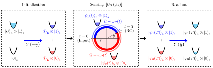
Figure 1: (Color online) Schematic protocol of Sagnac interferometer with trapped atomic clock states for rotation sensing Stevenson et al. (2015). The protocol consists of initialization, sensing and readout, where $Y\left(\pm\pi/2\right)$ denotes the $\pi/2$ pulses and the clock states are $\left|0\right\rangle_{\mathrm{s}}=\left|\uparrow\right\rangle$ and $\left|1\right\rangle_{\mathrm{s}}=\left|\downarrow\right\rangle$, respectively, and $\left|{\cal{G}}\right\rangle_{\mathrm{h}}$ is the ground state of atoms in the harmonic trap, with the subscript $\mathrm{h}$ ($\mathrm{s}$) denoting the harmonic oscillator (spin) subspace. In the sensing period, the atoms in two traps are coherently split at $t=0$ and are counter-transported along a circular path of radius $r$ with respective angular velocity $\Omega\pm\omega_{P}(t)$ in the inertial frame ${\cal{K}}$, and are recombined (RC) at time $T$. By properly designing the $\omega_{P}(t)$ profile and the interrogation time $T$, a Sagnac phase gate $U_{S}\left(\phi_{S}\right)$ can be obtained, where $\phi_{S}=2\pi mr^{2}\Omega/\hbar$ is the Sagnac phase. The rotation frequency $\Omega$ can be read out from the population information after applying another $\pi/2$ pulse in the readout stage.

II Model and Interferometer Phase

Within the basic scheme in Ref. Stevenson et al. (2015), the interferometer protocol consists of two Ramsey $\pi/2$ pulses and two identical harmonic traps which counter-transport the clock states $\left|\uparrow\right\rangle$ and $\left|\downarrow\right\rangle$ along circular paths of radius $r$ in the $xy$ plane, with respective sweeping angular velocity $\pm\omega_{P}(t){\bf{z}}$ [$\omega_{P}(t)\geq 0$] in the rotating frame $\cal{R}$. And $\cal{R}$ rotates in an angular velocity ${\bf{\Omega}}=\Omega{\bf{z}}$ with respect to an inertial frame ${\cal{K}}$. See Fig. 1 for a schematic illustration. The interrogation time $T$, when the two components are recombined for readout, is given by $\int_{0}^{T}\omega_{P}(t)\mathrm{d}t=\pi$. The unitary time-evolution operators $U_{\uparrow}(T)$ and $U_{\downarrow}(T)$ for the two respective paths form a Sagnac phase-encoding gate $U_{S}\left(\phi_{S}\right)$ at $t=T$, which imprints the Sagnac phase into the qubit phase. Formally, the interferometer protocol can be written as Ref

$$V(T)=Y\left(\frac{\pi}{2}\right)U(T)Y\left(-\frac{\pi}{2}\right),$$ (1)

where $Y\left(\phi\right)=\mathrm{exp}\left(-i\phi\sigma_{y}/2\right)$ with $\sigma_{y}$ being the Pauli matrix, and $U(T)={\cal{T}}\mathrm{exp}\left[-i\int_{0}^{T}H(t)\mathrm{d}t/\hbar\right]$ with ${\cal{T}}$ being the time ordering operator and $H(t)=H_{0}(t)\Pi_{0}+H_{1}(t)\Pi_{1}$ being the Hamiltonian, where we have used the notation $\left|0\right\rangle_{\mathrm{s}}\left(\left|1\right\rangle_{\mathrm{s}}\right)=\left|\uparrow\right\rangle\left(\left|\downarrow\right\rangle\right)$ and $\Pi_{0}\left(\Pi_{1}\right)=\left|0\right\rangle_{\mathrm{ss}}\left\langle 0\right|\left(\left|1\right\rangle_{\mathrm{ss}}\left\langle 1\right|\right)$, with the subscript $\mathrm{s}$ denoting the (pseudo)spin subspace. It can be shown directly that (See Appendix A)

$$U(T)=U_{0}(T)\Pi_{0}+U_{1}(T)\Pi_{1},$$ (2)

where $U_{\eta}(T)={\cal{T}}\mathrm{exp}\left[-i\int_{0}^{T}H_{\eta}(t)\mathrm{d}t/\hbar\right]$ for $\eta=0,1$ and $H_{\eta}(t)$ is the time dependent single component Hamiltonian.

For the Sensing period in the interferometer scheme shown in Fig. 1, if the degrees of freedom in the axial and radial directions for atoms in the harmonic trap are tightly confined, then the time evolution can be described by the one-dimensional model in Ref. Stevenson et al. (2015), where the Hamiltonian for the $\left|\eta\right\rangle_{\mathrm{s}}$ state atoms in the stationary reference frame relative to the transporting harmonic trap is given by

$$H_{\eta}(t)=\hbar\omega_{0}\left(a^{\dagger}a+\frac{1}{2}\right)+i\lambda_{\eta}(t)\left(a-a^{\dagger}\right),$$ (3)

where $\omega_{0}$ is the trap frequency and $a\left(a^{\dagger}\right)$ is the annihilation (creation) operator for the trap mode. The second term in Eq. (3) represents the drive acting on the harmonic oscillator induced by the rotation of the frame, where $\lambda_{\eta}(t)=\sqrt{\frac{m\hbar\omega_{0}}{2}}r\left[\Omega+(1-2\eta)\omega_{P}(t)\right]$, with $m$ being the particle mass and $\Omega$ the rotation frequency to be measured. $\omega_{P}(t)\geq 0$ for $t\in[0,T]$ is the experimentally designed sweeping angular velocity whose temporal profile determines the interferometer phase and the signal contrast, which will be shown below. The sweeping angular velocity $\omega_{P}(t)$ can be further extended to a function ${\cal{W}}_{P}(t)$ defined on the whole real-time axis $t\in\left[-\infty,+\infty\right]$, with ${\cal{W}}_{P}(t)=\omega_{P}(t)$ for $t\in[0,T]$ and ${\cal{W}}_{P}(t)=0$ for the other, and the frequency spectrum of ${\cal{W}}_{P}(t)$ can be obtained from its Fourier transform

$$\widetilde{{\cal{W}}}_{P}(\omega)=\frac{1}{\sqrt{2\pi}}\int_{-\infty}^{+\infty}{\cal{W}}_{P}(t)\mathrm{exp}\left(-i\omega t\right)\mathrm{d}t.$$ (4)

The Hamiltonian in Eq. (3) describes a driven harmonic oscillator and the corresponding time evolution operator at time $t$ is given by (see Appendix A for detailed derivations)

$$U_{\eta}(t)=D\left[\alpha_{\eta}(t)\right]e^{-i\omega_{0}a^{\dagger}at}e^{i\left[\phi_{\eta}(t)-\omega_{0}t/2\right]},$$ (5)

where $D\left(\alpha\right)=\mathrm{exp}\left(\alpha a^{\dagger}-\alpha^{*}a\right)$ is the displacement operator for the harmonic oscillator, with

$$\alpha_{\eta}(t) = -\frac{1}{\hbar}\int^{t}_{0}\lambda_{\eta}(\tau)\mathrm{exp}\left[i\omega_{0}\left(\tau-t\right)\right]\mathrm{d}\tau,$$

$$\phi_{\eta}(t) = \frac{1}{\hbar^{2}}\int_{0}^{t}\int_{0}^{\tau_{1}}\lambda_{\eta}(\tau_{1})\lambda_{\eta}(\tau_{2})\sin\left[\omega_{0}\left(\tau_{1}-\tau_{2}\right)\right]\mathrm{d}\tau_{2}\mathrm{d}\tau_{1}.$$

If the initial states for both $\left|0\right\rangle_{\mathrm{s}}$ and $\left|1\right\rangle_{\mathrm{s}}$ components in the harmonic trap are in the ground state (vacuum) $\left|{\cal{G}}\right\rangle_{\mathrm{h}}$ which is defined by $a\left|{\cal{G}}\right\rangle_{\mathrm{h}}=0$, where the subscript ${\mathrm{h}}$ denotes the harmonic trap subspace, then the state at time $t$ is given by

$$\left|\psi_{\eta}(t)\right\rangle_{\mathrm{h}} = U_{\eta}(t)\left|{\cal{G}}\right\rangle_{\mathrm{h}}$$ (7)

$$= \left|\alpha_{\eta}(t)\right\rangle_{\mathrm{h}}\mathrm{exp}\left[i\left(\phi_{\eta}(t)-\omega_{0}t/2\right)\right],$$

where $\left|\alpha_{\eta}(t)\right\rangle_{\mathrm{h}}$ is the coherent state which is eigenstate of $a$ with eigenvalue $\alpha_{\eta}(t)$. See the sensing period in Fig. 1.

For the initial state $\rho(0)=\left|{\cal{G}}\right\rangle_{\mathrm{hh}}\left\langle{\cal{G}}\right|\otimes\left|1\right\rangle_{\mathrm{ss}}\left\langle 1\right|$ of the interferometer, the readout state reads $\rho(T)=V(T)\rho(0)V^{\dagger}(T)$. The reduced density matrix for the spin subspace is given by $\rho_{\mathrm{s}}(T)=\mathrm{Tr_{h}}\rho(T)$ with $\mathrm{Tr}$ being the trace operation, and reads

$$\rho_{\mathrm{s}}(T)=\frac{1}{2}\left[{\cal{I}}_{2}-\mathrm{Re}\left({\cal{C}}_{1,0}\right)\sigma_{z}-\mathrm{Im}\left({\cal{C}}_{1,0}\right)\sigma_{y}\right],$$ (8)

where ${\cal{I}}_{2}$ is the two-dimensional identity matrix, ${\cal{C}}_{j,k}={}_{\mathrm{h}}\left\langle\alpha_{j}(T)|\alpha_{k}(T)\right\rangle_{\mathrm{h}}\mathrm{exp}\left\{-i\left[\phi_{j}(T)-\phi_{k}(T)\right]\right\}$ with $j,k\in\{0,1\}$ and $\mathrm{Re}\left(\mathrm{Im}\right)$ denotes the real (imaginary) part. $\sigma_{z}=\left|0\right\rangle\left\langle 0\right|-\left|1\right\rangle\left\langle 1\right|$ and $\sigma_{y}=i\left(\left|1\right\rangle\left\langle 0\right|-\left|0\right\rangle\left\langle 1\right|\right)$ are the Pauli operators. Therefore, the measurement signal, e.g., the population difference, is given by

$$\quad_{\mathrm{s}}\left\langle\sigma_{z}\right\rangle_{\mathrm{s}}=-|{\cal{C}}_{1,0}|\mathrm{cos}\left(\phi_{I}\right),$$ (9)

where the modulus $|{\cal{C}}_{1,0}|=\mathrm{exp}\left(-|\Delta\alpha|^{2}/2\right)$ gives the signal contrast, with $\Delta\alpha=\alpha_{0}(T)-\alpha_{1}(T)\propto\widetilde{{\cal{W}}}_{P}^{*}\left(\omega_{0}\right)$, and $\phi_{I}=\mathrm{arg}\left({\cal{C}}_{1,0}\right)$ is the interferometer phase, with $\mathrm{arg}$ denoting the argument. From straightforward calculation one obtains the interferometer phase $\phi_{I}$, which is given by (see Appendix B)

$$\phi_{I}=\phi_{S}\left\{1-\sqrt{\frac{2}{\pi}}\mathrm{Re}\left[\widetilde{{\cal{W}}}_{P}\left(\omega_{0}\right)\right]\right\},$$ (10)

where $\phi_{S}=2\pi mr^{2}\Omega/\hbar$ is the well-known Sagnac phase and it can be further shown that $0\leq\phi_{I}\leq 2\phi_{S}$. In contrast to Ref. Stevenson et al. (2015), the phase of the interferometer in Eq. (9) is indeed dependent on the Fourier components of $\widetilde{{\cal{W}}}_{P}\left(\omega\right)$ at the trap frequency $\omega_{0}$ and therefore depends on the temporal profile of $\omega_{P}(t)$. This result is experimentally relevant because the form of $\omega_{P}(t)$ profile will affect the interference fringes. Now we arrive at the condition

$$\mathrm{Re}\left[\widetilde{{\cal{W}}}_{P}\left(\omega_{0}\right)\right]=0,$$ (11)

under which $\phi_{I}=\phi_{S}$, i.e., the interferometer phase is exactly the Sagnac phase.

It should be noted that Eq. (11) could be satisfied when the guiding procedure is performed in an adiabatic fashion, i.e., $T\gg 2\pi/\omega_{0}$. For example, for a constant $\omega_{P}(t)=\pi/T$, we have $\mathrm{Re}\left[\widetilde{{\cal{W}}}_{P}\left(\omega\right)\right]=\sqrt{\pi/2}\mathrm{sin}\left(\omega T\right)/\left(\omega T\right)$. Consequently, the amplitude of the frequency distribution decreases with $\omega$ in power law and for large $\omega_{0}$ located far away from the typical spectrum width of the order $1/T$, the contribution from the real part in Eq. (10) approaches $0$. On the other hand, for nonadiabatic guiding procedures with $T\sim\omega_{0}^{-1}$ (if possible in future experiments), the sweeping angular velocity and the interrogation time should be properly designed such that $\omega_{0}$ lies in the node of the frequency spectrum.

III Phase-Space Geometric Sagnac Interferometers

Up to now we have obtained the relationship between the interferometer phase and the Sagnac phase, but the dynamic and geometric origins of the phase in the phase space have not been investigated yet. Next we analyze different components in the Sagnac phase $\phi_{S}$ and explore unconventional geometric Zhu and Wang (2003); Du et al. (2006) Sagnac interferometers, which could be potentially resilient to noises and are promising for reaching high-precision quantum rotation sensing.

Quantum geometric phase is the phase change associated with holonomic transformation in quantum state space Simon (1983); Anandan and Stodolsky (1987); Aharonov and Anandan (1987); Song et al. (2017), which was studied by Berry Berry (1984) for adiabatic cyclic motion and by Aharonov and Anandan Aharonov and Anandan (1987) for any cyclic evolution. Here for the spin state $\left|\eta\right\rangle_{\mathrm{s}}$ ($\eta=0,1$), the total phase change for quantum evolution in each harmonic trap can be divided into dynamic and geometric components, which are given by Zhu and Wang (2003); Carollo et al. (2003)

$$\gamma^{\mathrm{d}}_{\eta}(T)=-\int_{0}^{T}\left\langle\psi_{\eta}(t)|H_{\eta}(t)|\psi_{\eta}(t)\right\rangle\mathrm{d}t,$$ (12)

and

$$\gamma^{\mathrm{g}}_{\eta}(T)=\frac{i}{2}\int_{\Gamma_{\eta}}\left(\alpha_{\eta}^{*}\mathrm{d}\alpha_{\eta}-\alpha_{\eta}\mathrm{d}\alpha^{*}_{\eta}\right)-\mathrm{arg}\left[\left\langle\alpha_{\eta}(T)|{\cal{G}}\right\rangle\right],$$

respectively. Note that here in Eqs. (12) (III) and hereafter we will drop the subspace subscript $\mathrm{h}$ for convenience. From Eq. (III), one sees that the geometric phase consists of two parts, where the first is $-2$ times the area Dou subtended by the path $\Gamma_{\eta}=\{\alpha_{\eta}(t)|t\in[0,T]\}$ of motion in the phase space and the second is the argument of the overlap between the initial and final coherent states. Define $\Delta\gamma^{\mathrm{d(g)}}=\gamma_{0}^{\mathrm{d(g)}}(T)-\gamma_{1}^{\mathrm{d(g)}}(T)$ as the dynamic (geometric) phase difference of the interferometer, which satisfies $\phi_{I}=\Delta\gamma^{\mathrm{d}}+\Delta\gamma^{\mathrm{g}}+\mathrm{arg}\left[\left\langle\alpha_{1}(T)|\alpha_{0}(T)\right\rangle\right]$. The third component in $\phi_{I}$ is given by $\mathrm{arg}\left[\left\langle\alpha_{1}(T)|\alpha_{0}(T)\right\rangle\right]=|\alpha_{0}(T)\alpha^{*}_{1}(T)|\mathrm{sin}\left\{\mathrm{arg}\left[\alpha_{0}(T)\right]-\mathrm{arg}\left[\alpha_{1}(T)\right]\right\}$, which only depends on the respective final positions of the $\left|0\right\rangle$ and $\left|1\right\rangle$ state atoms in the trap when they are recombined, and also has a clear geometric meaning. Therefore, it can be absorbed into the geometric phase difference. Consequently, the total phase difference of the Sagnac interferometer in Eq. (10) can be decomposed into

$$\phi_{I}=\Delta\gamma^{\mathrm{d}}+\Delta\tilde{\gamma}^{\mathrm{g}},$$ (14)

where $\Delta\tilde{\gamma}^{\mathrm{g}}=\gamma_{0}^{\mathrm{g}}(T)-\gamma_{1}^{\mathrm{g}}(T)+\mathrm{arg}\left[\left\langle\alpha_{1}(T)|\alpha_{0}(T)\right\rangle\right]$ is the purely geometric contribution related to the area and angle differences in the phase spaces, respectively.

Next, with a theorem, we show that by properly designing the interrogation time $T$ and the temporal profile of the sweeping angular velocity $\omega_{P}(t)$, the Sagnac phase can be made a pure or unconventional geometric phase, where by the latter we mean that the geometric Sagnac phase also involves a dynamic component Zhu and Wang (2003). We give criteria for the phase-space geometric Sagnac phase, followed by proposed experimentally accessible schemes for geometric Sagnac interferometers.

Theorem. For certain proper interrogation time $T$ and temporal profiles of $\omega_{P}(t)\geq 0$ with $t\in[0,T]$ which satisfy $\phi_{I}=\phi_{S}$, there exist nonzero $\kappa\in\mathbb{R}$ such that

$$\Delta\gamma^{\mathrm{d}}=\left(\kappa-1\right)\Delta\tilde{\gamma}^{\mathrm{g}},$$ (15)

where for $\kappa=1$, the Sagnac phase $\phi_{S}$ is purely geometric, and for $\kappa\neq 1$, $\phi_{S}$ is an unconventional geometric phase Int .

Proof and examples. With the frequency spectrum $\widetilde{{\cal{W}}}_{P}\left(\omega\right)$ and straightforward calculations we obtain (see Appendix C for detailed calculations)

$$\Delta\tilde{\gamma}^{\mathrm{g}}=\sqrt{\frac{2}{\pi}}\phi_{S}\xi\left(\omega_{0},T\right),\ \ \ \Delta\gamma^{\mathrm{d}}=\phi_{I}-\Delta\tilde{\gamma}^{\mathrm{g}},$$ (16)

where $\phi_{I}$ is given by Eq. (10) and $\xi\left(\omega_{0},T\right)=\omega_{0}\partial_{\omega}\mathrm{Re}\left[\widetilde{{\cal{W}}}_{P}\left(\omega\right)\right]_{\omega=\omega_{0}}-\omega_{0}T\mathrm{Im}\left[\widetilde{{\cal{W}}}_{P}\left(\omega_{0}\right)\right]$.

Under the condition $\phi_{I}=\phi_{S}$ and maximization of the contrast, which indicate $\widetilde{{\cal{W}}}_{P}\left(\omega_{0}\right)=0$, $\kappa$ in Eq. (15) can be expressed as

$$\kappa=\sqrt{\pi/2}/\xi_{0}\left(\omega_{0},T\right),$$ (17)

with $\xi_{0}\left(\omega_{0},T\right)=\omega_{0}\partial_{\omega}\mathrm{Re}\left[\widetilde{{\cal{W}}}_{P}\left(\omega\right)\right]_{\omega=\omega_{0}}$. Therefore, for properly designed $\omega_{P}(t)$ and $T$, if there exists nonzero $\xi_{0}\left(\omega_{0},T\right)$, then this theorem holds automatically. The unconventional geometric class with $\xi_{0}\left(\omega_{0},T\right)\neq\sqrt{\pi/2}$ should be more generic. Below we give two examples of this class with sinusoidal and cosinusoidal temporal profiles for $\omega_{P}(t)$, respectively, which could be schemes for the unconventional geometric Sagnac interferometer. A pure geometric scheme with flat $\omega_{P}(t)$ profile will also be presented in the following.

(i) Unconventional geometric Sagnac phase. Firstly we present a designed sinusoidal angular velocity $\omega_{P}(t)=\pi^{2}|\mathrm{sin}\left(2\pi t/T\right)|/\left(2T\right)$ for $t\in[0,T]$ with $T=2\pi/\omega_{0}$, which sets $\phi_{I}=\phi_{S}$ and maximizes the contrast at the same time, i.e., $\widetilde{{\cal{W}}}_{P}\left(\omega_{0}\right)=0$ for this situation. This sinusoidal profile results in a nontrivial solution for $\kappa$ in Eq. (15), $\kappa=8/\pi^{2}$, and the Sagnac phase $\phi_{S}=8\Delta\tilde{\gamma}^{\mathrm{g}}/\pi^{2}$ (see Appendix D for detailed calculations) is an unconventional geometric phase, by which we mean that the geometric $\phi_{S}$ also involves a dynamic component Zhu and Wang (2003).

Secondly, we find that the cosinusoidal angular velocity profile (sinusoidal angular profile) used in Ref. Haine (2016) in order to calculate the Fisher information, may also provide a nontrivial scheme for the unconventional geometric Sagnac interferometer, where $\omega_{P}(t)=\left(\pi/T\right)\left[1-\mathrm{cos}\left(2\pi t/T\right)\right]$. By choosing the interrogation time to be $T=2M\pi/\omega_{0}$, where $M=2,3,4,...$, we have $\widetilde{{\cal{W}}}_{P}\left(\omega_{0}\right)=0$, and the corresponding $\kappa$ is given by $\kappa=1-M^{2}$. Therefore, the Sagnac phase $\phi_{S}=\left(1-M^{2}\right)\Delta\tilde{\gamma}^{\mathrm{g}}$ (see Appendix D) is also an unconventional geometric phase. It is worth noting that the former sinusoidal profile case can only be performed in a nonadiabatic guiding procedure due to $T\sim\omega_{0}^{-1}$, while the latter cosinusoidal case is applicable to both adiabatic and nonadiabatic scenarios, which depends on the value of $M$ taken in $T\sim M\omega_{0}^{-1}$.

(ii) Pure geometric Sagnac phase. A constant angular velocity $\omega_{P}(t)=\pi/T$ for $t\in[0,T]$ with $T=2K\pi/\omega_{0}$ gives $\widetilde{{\cal{W}}}_{P}\left(\omega_{0}\right)=0$, where $K=1,2,3,\cdots$, and therefore $\phi_{I}=\phi_{S}$ and the contrast is maximized simultaneously. The solution for $\kappa$ in Eq. (15) is $\kappa\equiv 1$ (see Appendix D). Furthermore, in this example $\gamma_{\eta}^{\mathrm{d}}(T)=-K\pi$ for both branches with $\eta=0$ and $1$, which comes from the zero-energy contribution. So the Sagnac phase in this case is purely geometric.

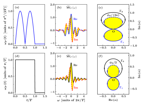
Figure 2: (Color online) Unconventional [(a)–(c)] and pure [(d)–(f)] geometric Sagnac interferometers with atomic clock states, where (a) and (d), (b) and (e), (c) and (f) share the same horizontal axis labels, respectively. (a) is the sinusoidal $\omega_{P}(t)$ profile [in units of $\pi^{2}/(2T)$] in the example (i) and (d) is the flat $\omega_{P}(t)$ profile (in units of $\pi/T$) in the example (ii). (b) and (e) are Fourier transform $\widetilde{{\cal{W}}}_{P}\left(\omega\right)$ of (a) and (d), respectively, where $\mathrm{Re}$ ($\mathrm{Im}$) denotes the real (imaginary) part. The horizontal frequency axes in both (b) and (e) are in units of $2\pi/T$. (c) and (f) are the phase space paths for the atoms in the two respective traps during the interrogation, where $\Gamma_{\eta}=\{\alpha_{\eta}(t)|t\in[0,T]\}$ is the path of $\left|\eta\right\rangle_{\mathrm{s}}$ state atoms in the $\alpha$ plane with $\eta=0$ and $1$, respectively. (c) is plotted with the sinusoidal $\omega_{P}(t)$ profile in (a), and (f) is with the flat profile in (d). For both (c) and (f), we take $\omega_{0}=\hbar=m=r=1$, $\Omega=0.1\omega_{0}$ and $T=2\pi/\omega_{0}$, and the dashed blue line denotes $-\Gamma_{1}=\{-\alpha_{1}(t)|t\in[0,T]\}$ which encloses the same area as $\Gamma_{1}$. The area of the unfilled region inside $\Gamma_{0}$ is proportional to $\phi_{S}/2$ in (c) with $\kappa=8/\pi^{2}$, while it is identical with $\phi_{S}/2$ in (f).

The physical pictures for above schemes are as follows: When the two branches are recombined at $t=T$, the atoms in each trap accomplish integer numbers of cyclic evolutions, and return to the initial vacuum state, during which the Sagnac phase is given by the area difference subtended by the two trajectories in the phase spaces. Figures  2(a)–2(c) plot the unconventional geometric Sagnac phase with the sinusoidal $\omega_{P}(t)$ profile and Figs. 2(d)–2(f) show the pure geometric counterpart with the flat $\omega_{P}(t)$ profile. In Figs. 2(b) and 2(e), to satisfy $\phi_{I}=\phi_{S}$ and to maximize the contrast at the same time, the trap frequency $\omega_{0}$ is given by the positive simultaneous zeros of real ($\mathrm{Re}$) and imaginary ($\mathrm{Im}$) parts of $\widetilde{{\cal{W}}}_{P}\left(\omega\right)$, which is $\omega_{0}T=2\left(2L+1\right)\pi$ for Fig. 2 (b) with $L=0,1,2,\cdots$, and $\omega_{0}T=2K\pi$ for Fig. 2(e) with $K$ being a positive integer (see Appendix D). Shown in Figs. 2(c) and 2(f) are the phase space paths $\Gamma_{\eta}$ for $\left|\eta\right\rangle_{\mathrm{s}}$ state atoms during the interrogation, with $\eta=0$ and $1$, respectively. Fig. 2(c) is plotted with the sinusoidal $\omega_{P}(t)$ profile and $L=0$, and Fig. 2(f) is with the flat profile and $K=1$. Note that in Fig. 2(b), only the $L=0$ case can give a nontrivial solution for $\kappa$ in Eq. (15). The dashed blue line denotes $-\Gamma_{1}=\{-\alpha_{1}(t)|t\in[0,T]\}$ which encloses the same area as $\Gamma_{1}$. Therefore, the area of the unfilled region inside $\Gamma_{0}$, which is equal to $\Delta\tilde{\gamma}^{\mathrm{g}}/2$, is identical with $\phi_{S}/\left(2\kappa\right)$ with $\kappa=8/\pi^{2}$ in Fig. 2(c) while it equals $\phi_{S}/2$ in Fig. 2(f), which are signatures of unconventional and pure geometric Sagnac phases, respectively.

So we have provided criteria for geometric Sagnac interferometers in the phase space and proposed corresponding schemes for geometric quantum rotation sensing with trap-guided atomic clocks. It should be noted that in the completely adiabatic regime with $T\gg\omega_{0}^{-1}$, the unconventional geometric phase component given by the cosinusoidal $\omega_{P}(t)$ in example (i) is $\Delta\tilde{\gamma}^{\mathrm{g}}\propto\kappa^{-1}\approx 0$, and $\phi_{S}$ becomes nearly completely dynamic. In this regime, the pure geometric scheme with flat $\omega_{P}(t)\propto T^{-1}$ in example (ii) is more accessible in experiments due to the fact that $\kappa\equiv 1$ for this scheme. In nonadiabatic and intermediate regimes, the unconventional geometric schemes in example (i) could be more accessible due to continuous $\omega_{P}(t)$ with $\omega_{P}(0)=\omega_{P}(T)=0$.

IV Precision and Sensitivity

Now we discuss the precision and sensitivity of the above schemes. The sensitivity of the Sagnac interferometer is limited by the uncertainty of the unbiased estimated value of $\Omega$, which is given by $\delta\Omega=\delta P\left(\phi_{I}\right)/\left|\partial_{\Omega}P\left(\phi_{I}\right)\right|$, where $P\left(\phi_{I}\right)=_{\mathrm{s}}\left\langle\sigma_{z}\right\rangle_{\mathrm{s}}$ is the signal given in Eq. (9). Straightforward calculation leads to

$$\frac{1}{\left(\delta\Omega\right)^{2}}=\frac{\left(\frac{\partial\phi_{I}}{\partial\Omega}\right)^{2}\mathrm{sin}^{2}\phi_{I}}{\left|{\cal{C}}_{1,0}\right|^{-2}-1+\mathrm{sin}^{2}\phi_{I}}\leq{\cal{F}},$$ (18)

where we have $\left|{\cal{C}}_{1,0}\right|\leq 1$ and ${\cal{F}}$ is the quantum Fisher information (QFI) which determines the ultimate precision limit for quantum sensing via the quantum Cramér-Rao bound (QCRB) Helstrom (1976); Holevo (1982). For the interferometer protocol $V(T)$ and the initial state $\rho(0)$ in this paper, if the interrogation time is integer times the trap period, i.e., $T=2K\pi/\omega_{0}$ with $K=1,2,3,\cdots$, then the QFI in Eq. (18) is given by ${\cal{F}}=\left(\partial_{\Omega}\phi_{I}\right)^{2}$  Yao et al. . Therefore, the conditions for attaining the equality in Eq. (18) and saturating the QCRB are $\left|{\cal{C}}_{1,0}\right|=1$ [or $\widetilde{{\cal{W}}}_{P}\left(\omega_{0}\right)=0$] and $\omega_{0}T=2K\pi$. So all the schemes proposed in the examples (i) and (ii) with $P\left(\phi_{I}\right)$ measurements satisfy these conditions and thus saturate the QCRB.

V Conclusion

In summary, we have proposed schemes for phase-space geometric Sagnac interferometers with trap-guided atomic clocks, which could be potentially noise resilient and promising for high-sensitivity rotation sensors. The pure geometric scheme is applicable to adiabatic guiding procedures while the unconventional geometric schemes could be more accessible in nonadiabatic situations. In addition, the established relationship between the interferometer phase and the Sagnac phase may provide a theoretical basis of evaluating the scale factor for the Sagnac interferometer, which is crucial for the accuracy of atomic sensors.

It is also worth noting that in realistic experiments, the initial states in both harmonic traps are usually identical mixed thermal states as discussed in Ref. Stevenson et al. (2015), and if the manipulation of atoms in the phase space during the interrogation is a cyclic evolution of the mixed state with respect to the center of the probability distribution, then the finite temperature does not affect both the contrast and the geometric Sagnac phase, where the latter is proportional to the area difference of the two enclosed trajectories in the phase space. This result shows that the proposed geometric rotation sensing schemes are not restricted to zero temperature and the initial single-particle ground state in the harmonic trap. Our work could stimulate further interests and studies on phase-space geometric quantum sensing with guided matter waves.

Appendix A Derivation of the time-evolution operator $U_{\eta}(t)$ in Eq. (5)

Here we give the detailed derivations of the total time-evolution operator $U(t)$ and the single-component time-evolution operator $U_{\eta}(t)$ in Eq. (5). With the properties of projection operators, $\Pi_{i}\Pi_{j}=\delta_{ij}\Pi_{i}$ for $i,j\in\{0,1\}$, one can obtain

$$U(T) = {\cal{T}}\mathrm{exp}\left[-i\int_{0}^{T}H(t)\mathrm{d}t/\hbar\right]$$ (19)

$$= {\cal{I}}_{\mathrm{h}}\otimes{\cal{I}}_{\mathrm{s}}+\left(-i/\hbar\right)\int_{0}^{T}H(t)\mathrm{d}t+\sum_{k=2}^{\infty}\frac{\left(-i/\hbar\right)^{k}}{k!}\int_{0}^{T}\mathrm{d}t_{0}\int_{0}^{t_{0}}\mathrm{d}t_{1}\cdot\cdot\cdot\int_{0}^{t_{k-2}}\mathrm{d}t_{k-1}H\left(t_{0}\right)H\left(t_{1}\right)\cdot\cdot\cdot H\left(t_{k-1}\right)$$

$$= {\cal{I}}_{\mathrm{h}}\otimes{\cal{I}}_{\mathrm{s}}+\left\{{\cal{T}}\mathrm{exp}\left[-i\int_{0}^{T}H_{0}(t)\mathrm{d}t/\hbar\right]-{\cal{I}}_{\mathrm{h}}\right\}\Pi_{0}+\left\{{\cal{T}}\mathrm{exp}\left[-i\int_{0}^{T}H_{1}(t)\mathrm{d}t/\hbar\right]-{\cal{I}}_{\mathrm{h}}\right\}\Pi_{1}$$

$$= U_{0}(T)\Pi_{0}+U_{1}(T)\Pi_{1},$$

where ${\cal{I}}$ is the identity operator and $U_{\eta}(T)={\cal{T}}\mathrm{exp}\left[-i\int_{0}^{T}H_{\eta}(t)\mathrm{d}t/\hbar\right]$ for $\eta\in\{0,1\}$, with $H_{\eta}(t)$ being the time-dependent single-component Hamiltonian for the harmonic oscillator mode, and we have used the relation $\Pi_{0}+\Pi_{1}={\cal{I}}_{\mathrm{s}}$.

The Hamiltonian in Eq. (3) describes a forced harmonic oscillator and the corresponding time-evolution operator at time $t$ can be written as

$$U_{\eta}(t)=U_{(0)}(t){\cal{U}}_{\eta}(t),$$ (20)

where $U_{(0)}(t)=\mathrm{exp}\left[-i\omega_{0}\left(a^{\dagger}a+\frac{1}{2}\right)t\right]$ and ${\cal{U}}_{\eta}(t)$ satisfies

$$i\hbar\frac{\partial}{\partial t}{\cal{U}}_{\eta}(t)=i\lambda_{\eta}(t)\left[\tilde{a}(t)-\tilde{a}^{\dagger}(t)\right]{\cal{U}}_{\eta}(t),$$ (21)

where $\tilde{a}(t)=a\mathrm{exp}\left(-i\omega_{0}t\right)$. Eq. (21) can be solved from the Magnus expansion Blanes et al. (2009) and is given by

$${\cal{U}}_{\eta}(t)=D\left[\beta_{\eta}(t)\right]\mathrm{exp}\left[i\phi_{\eta}(t)\right],$$ (22)

where $\beta_{\eta}(t)=-\int^{t}_{0}\lambda_{\eta}(\tau)\mathrm{exp}(i\omega_{0}\tau)\mathrm{d}\tau/\hbar$,

$$\phi_{\eta}(t)=\int_{0}^{t}\int_{0}^{\tau_{1}}\lambda_{\eta}(\tau_{1})\lambda_{\eta}(\tau_{2})\sin\left[\omega_{0}\left(\tau_{1}-\tau_{2}\right)\right]\mathrm{d}\tau_{2}\mathrm{d}\tau_{1}/\hbar^{2},$$ (23)

and $D\left(\beta\right)=\mathrm{exp}\left(\beta a^{\dagger}-\beta^{*}a\right)$ is the displacement operator for the oscillator. Therefore, the time evolution operator in Eq. (20) reads

$$U_{\eta}(t) = U_{(0)}(t)D\left[\beta_{\eta}(t)\right]U_{(0)}^{\dagger}(t)\mathrm{exp}\left(-i\omega_{0}a^{\dagger}at\right)\mathrm{exp}\left[i\left(\phi_{\eta}(t)-\omega_{0}t/2\right)\right]$$ (24)

$$= D\left[\alpha_{\eta}(t)\right]\mathrm{exp}\left(-i\omega_{0}a^{\dagger}at\right)\mathrm{exp}\left[i\left(\phi_{\eta}(t)-\omega_{0}t/2\right)\right],$$

which is Eq. (5) in the main text, with

$$\alpha_{\eta}(t)=\beta_{\eta}(t)\mathrm{exp}\left(-i\omega_{0}t\right)=-\int^{t}_{0}\lambda_{\eta}(\tau)\mathrm{exp}\left[i\omega_{0}\left(\tau-t\right)\right]\mathrm{d}\tau/\hbar.$$ (25)

Appendix B Derivation of the interferometer phase $\phi_{I}$ in Eq. (10)

In this appendix we present detailed calculations of the interferometer phase $\phi_{I}$ in Eq. (10), which establishes a relationship between $\phi_{I}$ and the well-known Sagnac phase. The ${\cal{C}}_{1,0}$ in the spin density matrix $\rho_{\mathrm{s}}(T)$ is given by

$${\cal{C}}_{1,0} = {}_{\mathrm{h}}\left\langle\alpha_{1}(T)|\alpha_{0}(T)\right\rangle_{\mathrm{h}}\mathrm{exp}\left\{-i\left[\phi_{1}(T)-\phi_{0}(T)\right]\right\}$$ (26)

$$= \mathrm{exp}\left(-|\Delta\alpha|^{2}/2\right)\mathrm{exp}\left\{i\left[\phi_{0}(T)-\phi_{1}(T)+\mathrm{Im}\left(\alpha_{1}^{*}(T)\alpha_{0}(T)\right)\right]\right\},$$

where $\Delta\alpha=\alpha_{0}(T)-\alpha_{1}(T)=-2r\sqrt{\pi m\omega_{0}/\hbar}\widetilde{{\cal{W}}}_{P}^{*}\left(\omega_{0}\right)\mathrm{exp}\left(-i\omega_{0}T\right)\propto\widetilde{{\cal{W}}}_{P}^{*}\left(\omega_{0}\right)$. In general, for an arbitrary time dependent function $\omega_{P}(t)$ which satisfies $\int_{0}^{T}\omega_{P}(\tau)\mathrm{d}\tau=\pi$, the explicit expression for $\phi_{\eta}(T)$ from Eq. (23) is difficult to obtain. Whereas, in terms of $\widetilde{{\cal{W}}}_{P}\left(\omega_{0}\right)$, the phase difference and the imaginary part in Eq. (26) have explicit forms, which are given by

$$\phi_{0}(T)-\phi_{1}(T) = \int_{0}^{T}\int_{0}^{\tau_{1}}\left[\lambda_{0}(\tau_{1})\lambda_{0}(\tau_{2})-\lambda_{1}(\tau_{1})\lambda_{1}(\tau_{2})\right]\sin\left(\omega_{0}\left(\tau_{1}-\tau_{2}\right)\right)\mathrm{d}\tau_{2}\mathrm{d}\tau_{1}/\hbar^{2}$$ (27)

$$= \left(m\omega_{0}\Omega r^{2}/\hbar\right)\int_{0}^{T}\int_{0}^{\tau_{1}}\left[\omega_{P}(\tau_{1})+\omega_{P}(\tau_{2})\right]\sin\left(\omega_{0}\left(\tau_{1}-\tau_{2}\right)\right)\mathrm{d}\tau_{2}\mathrm{d}\tau_{1}$$

$$= \left(m\Omega r^{2}/\hbar\right)\left[2\pi-\left(1+\mathrm{cos}\omega_{0}T\right)\int_{0}^{T}\omega_{P}(\tau)\mathrm{cos}\omega_{0}\tau\mathrm{d}\tau-\mathrm{sin}\omega_{0}T\int_{0}^{T}\omega_{P}(\tau)\mathrm{sin}\omega_{0}\tau\mathrm{d}\tau\right]$$

$$= \phi_{S}\left\{1-\frac{1}{\sqrt{2\pi}}\mathrm{Re}\left[\left(1+\mathrm{e}^{i\omega_{0}T}\right)\widetilde{{\cal{W}}}_{P}\left(\omega_{0}\right)\right]\right\},$$

and

$$\mathrm{Im}\left(\alpha_{1}^{*}(T)\alpha_{0}(T)\right) = \int_{0}^{T}\int_{0}^{T}\lambda_{0}(\tau_{1})\lambda_{1}(\tau_{2})\sin\left(\omega_{0}\left(\tau_{1}-\tau_{2}\right)\right)\mathrm{d}\tau_{2}\mathrm{d}\tau_{1}/\hbar^{2}$$ (28)

$$= \left[m\omega_{0}\Omega r^{2}/\left(2\hbar\right)\right]\int_{0}^{T}\int_{0}^{T}\left[\omega_{P}(\tau_{1})-\omega_{P}(\tau_{2})\right]\sin\left(\omega_{0}\left(\tau_{1}-\tau_{2}\right)\right)\mathrm{d}\tau_{2}\mathrm{d}\tau_{1}$$

$$= -\left(m\Omega r^{2}/\hbar\right)\left[\left(1-\mathrm{cos}\omega_{0}T\right)\int_{0}^{T}\omega_{P}(\tau)\mathrm{cos}\omega_{0}\tau\mathrm{d}\tau-\mathrm{sin}\omega_{0}T\int_{0}^{T}\omega_{P}(\tau)\mathrm{sin}\omega_{0}\tau\mathrm{d}\tau\right]$$

$$= \frac{\phi_{S}}{\sqrt{2\pi}}\mathrm{Re}\left[\left(\mathrm{e}^{i\omega_{0}T}-1\right)\widetilde{{\cal{W}}}_{P}\left(\omega_{0}\right)\right],$$

respectively, where $\phi_{S}=2m\pi r^{2}\Omega/\hbar$ is the Sagnac phase and we have used the relation

$$\int_{0}^{T}\int_{0}^{\tau_{1}}\omega_{P}(\tau_{2})\sin\left[\omega_{0}\left(\tau_{1}-\tau_{2}\right)\right]\mathrm{d}\tau_{2}\mathrm{d}\tau_{1} = \int_{0}^{T}\int_{\tau_{2}}^{T}\omega_{P}(\tau_{2})\sin\left[\omega_{0}\left(\tau_{1}-\tau_{2}\right)\right]\mathrm{d}\tau_{1}\mathrm{d}\tau_{2}$$ (29)

$$= \int_{0}^{T}\int_{\tau_{1}}^{T}\omega_{P}(\tau_{1})\sin\left[\omega_{0}\left(\tau_{2}-\tau_{1}\right)\right]\mathrm{d}\tau_{2}\mathrm{d}\tau_{1}.$$

Finally, the population difference, ${}_{\mathrm{s}}\left\langle\sigma_{z}\right\rangle_{\mathrm{s}}$, is given by

$$\quad{}_{\mathrm{s}}\left\langle\sigma_{z}\right\rangle_{\mathrm{s}} = \mathrm{Tr}_{\mathrm{s}}\left[\rho_{\mathrm{s}}(T)\sigma_{z}\right]$$ (30)

$$= -|{\cal{C}}_{1,0}|\mathrm{cos}\left(\phi_{I}\right),$$

where the modulus $|{\cal{C}}_{1,0}|=\mathrm{exp}\left(-|\Delta\alpha|^{2}/2\right)$ gives the signal contrast, and the interferometer phase is given by Eq. (26) and reads

$$\phi_{I} = \mathrm{arg}\left({\cal{C}}_{1,0}\right)$$ (31)

$$= \phi_{0}(T)-\phi_{1}(T)+\mathrm{Im}\left(\alpha_{1}^{*}(T)\alpha_{0}(T)\right)$$

$$= \phi_{S}\left\{1-\sqrt{\frac{2}{\pi}}\mathrm{Re}\left[\widetilde{{\cal{W}}}_{P}\left(\omega_{0}\right)\right]\right\}.$$

With the properties $\omega_{P}(t)\geq 0$ for $t\in[0,T]$, $\left|\cos\omega_{0}t\right|\leq 1$ and $\int_{0}^{T}\omega_{P}(t)\mathrm{d}t=\pi$, one can obtain $\left|\mathrm{Re}\left[\widetilde{{\cal{W}}}_{P}\left(\omega_{0}\right)\right]\right|\leq\sqrt{\pi/2}$. Therefore, we have $0\leq\phi_{I}\leq 2\phi_{S}$.

Appendix C Geometric and dynamic decomposition of the interferometer phase

Here we provide detailed calculations of the geometric and dynamic phase-difference components in $\phi_{I}$, which is Eq. (16). The dynamic and geometric phases $\gamma^{\mathrm{d}}_{\eta}(T)$ and $\gamma^{\mathrm{g}}_{\eta}(T)$ in each trap are given by

$$\gamma^{\mathrm{d}}_{\eta}(T) = -\int_{0}^{T}\left\langle\psi_{\eta}(t)|H_{\eta}(t)|\psi_{\eta}(t)\right\rangle\mathrm{d}t$$ (32)

$$= -\int_{0}^{T}\left[\omega_{0}\left(|\alpha_{\eta}(t)|^{2}+\frac{1}{2}\right)-\frac{2\lambda_{\eta}(t)}{\hbar}\mathrm{Im}\alpha_{\eta}(t)\right]\mathrm{d}t$$

$$= 2\phi_{\eta}(T)-\omega_{0}\int_{0}^{T}|\alpha_{\eta}(t)|^{2}\mathrm{d}t-\frac{1}{2}\omega_{0}T,$$

and

$$\gamma^{\mathrm{g}}_{\eta}(T) = \frac{i}{2}\int_{\Gamma_{\eta}}\alpha_{\eta}^{*}\mathrm{d}\alpha_{\eta}-\alpha_{\eta}\mathrm{d}\alpha^{*}_{\eta}-\mathrm{arg}\left[\left\langle\alpha_{\eta}(T)|{\cal{G}}\right\rangle\right]$$ (33)

$$= -\int_{0}^{T}\mathrm{Im}\left[\alpha_{\eta}^{*}(t)\partial_{t}\alpha_{\eta}(t)\right]\mathrm{d}t$$

$$= -\phi_{\eta}(T)+\omega_{0}\int_{0}^{T}|\alpha_{\eta}(t)|^{2}\mathrm{d}t,$$

respectively, where $\phi_{\eta}(T)$ is given by Eq. (23) and satisfies $\phi_{\eta}(T)-\omega_{0}T/2=\gamma^{\mathrm{d}}_{\eta}(T)+\gamma^{\mathrm{g}}_{\eta}(T)$, and $\mathrm{arg}\left[\left\langle\alpha_{\eta}(T)|{\cal{G}}\right\rangle\right]=0$.

In general, the calculations of explicit expressions for dynamic and geometric phases in each trap are difficult for an arbitrary $\lambda_{\eta}(t)$. Whereas, the dynamic and geometric phase differences $\Delta\gamma^{\mathrm{d}}$ and $\Delta\tilde{\gamma}^{\mathrm{g}}$ in Eq. (14) can be expressed in terms of $\widetilde{{\cal{W}}}_{P}\left(\omega\right)$ and its derivative at the trap frequency $\omega_{0}$, which will be shown below.

With $\omega_{0}\int_{0}^{T}|\alpha_{\eta}(t)|^{2}\mathrm{d}t=\left(\omega_{0}/\hbar^{2}\right)\int_{0}^{T}\mathrm{d}t\int_{0}^{t}\mathrm{d}\tau_{1}\int_{0}^{t}\mathrm{d}\tau_{2}\lambda_{\eta}(\tau_{1})\lambda_{\eta}(\tau_{2})\cos\omega_{0}\left(\tau_{1}-\tau_{2}\right)$, and by defining $\int_{0}^{T}\Delta|\alpha(t)|^{2}\mathrm{d}t=\int_{0}^{T}\left(|\alpha_{0}(t)|^{2}-|\alpha_{1}(t)|^{2}\right)\mathrm{d}t$, one can easily obtain

$$\omega_{0}\int_{0}^{T}\Delta|\alpha(t)|^{2}\mathrm{d}t = \left(\omega_{0}/\hbar^{2}\right)\int_{0}^{T}\mathrm{d}t\int_{0}^{t}\mathrm{d}\tau_{1}\int_{0}^{t}\mathrm{d}\tau_{2}\left[\lambda_{0}(\tau_{1})\lambda_{0}(\tau_{2})-\lambda_{1}(\tau_{1})\lambda_{1}(\tau_{2})\right]\cos\omega_{0}\left(\tau_{1}-\tau_{2}\right)$$

$$= \left(m\omega_{0}^{2}\Omega r^{2}/\hbar\right)\int_{0}^{T}\mathrm{d}t\int_{0}^{t}\mathrm{d}\tau_{1}\int_{0}^{t}\mathrm{d}\tau_{2}\left[\omega_{P}(\tau_{1})+\omega_{P}(\tau_{2})\right]\cos\omega_{0}\left(\tau_{1}-\tau_{2}\right)$$

$$= \phi_{S}\left\{1-\sqrt{\frac{2}{\pi}}\mathrm{Re}\left[\mathrm{e}^{i\omega_{0}T}\widetilde{{\cal{W}}}_{P}\left(\omega_{0}\right)\right]-\sqrt{\frac{2}{\pi}}\omega_{0}T\mathrm{Im}\left[\widetilde{{\cal{W}}}_{P}\left(\omega_{0}\right)\right]-\frac{\omega_{0}}{\pi}\int_{0}^{T}\tau\omega_{P}(\tau)\sin\omega_{0}\tau\mathrm{d}\tau\right\}$$

$$= \phi_{S}\left\{1-\sqrt{\frac{2}{\pi}}\mathrm{Re}\left[\mathrm{e}^{i\omega_{0}T}\widetilde{{\cal{W}}}_{P}\left(\omega_{0}\right)\right]-\sqrt{\frac{2}{\pi}}\omega_{0}T\mathrm{Im}\left[\widetilde{{\cal{W}}}_{P}\left(\omega_{0}\right)\right]+\sqrt{\frac{2}{\pi}}\omega_{0}\partial_{\omega}\mathrm{Re}\left[\widetilde{{\cal{W}}}_{P}\left(\omega\right)\right]_{\omega=\omega_{0}}\right\},$$

where we have used the same integration method as in Eq. (29) to obtain the third equation and we also have used the relation $\partial_{\omega}\mathrm{Re}\left[\widetilde{{\cal{W}}}_{P}\left(\omega\right)\right]_{\omega=\omega_{0}}=-\int_{0}^{T}\tau\omega_{P}(\tau)\sin\omega_{0}\tau\mathrm{d}\tau/\sqrt{2\pi}$. Together with Eqs. (27), (28), (32), and (33), we obtain

$$\Delta\tilde{\gamma}^{\mathrm{g}}=\sqrt{\frac{2}{\pi}}\phi_{S}\omega_{0}\left\{\partial_{\omega}\mathrm{Re}\left[\widetilde{{\cal{W}}}_{P}\left(\omega\right)\right]_{\omega=\omega_{0}}-T\mathrm{Im}\left[\widetilde{{\cal{W}}}_{P}\left(\omega_{0}\right)\right]\right\},$$ (35)

and

$$\Delta\gamma^{\mathrm{d}}=\phi_{S}\left\{1-\sqrt{\frac{2}{\pi}}\mathrm{Re}\left[\widetilde{{\cal{W}}}_{P}\left(\omega_{0}\right)\right]\right\}-\Delta\tilde{\gamma}^{\mathrm{g}},$$ (36)

respectively.

Appendix D Phase-space geometric Sagnac phase—Examples

Here we present several examples for the geometric Sagnac phases with designed $\omega_{P}(t)$ and the interrogation time $T$, with corresponding Fourier transform analyses.

Example (i): Unconventional geometric Sagnac phase. $(1)$ A sinusoidal angular velocity $\omega_{P}(t)=\pi^{2}|\mathrm{sin}\left(2\pi t/T\right)|/\left(2T\right)$ with $t\in[0,T]$ gives the Fourier transform

$$\mathrm{Re}\left[\widetilde{{\cal{W}}}_{P}\left(\omega\right)\right]=\frac{\sqrt{\pi/2}\cos^{2}\left(\frac{\omega T}{4}\right)\cos\left(\frac{\omega T}{2}\right)}{1-\left(\frac{\omega T}{2\pi}\right)^{2}},\ \ \ \mathrm{Im}\left[\widetilde{{\cal{W}}}_{P}\left(\omega\right)\right]=\frac{-\sqrt{2\pi}\cos^{3}\left(\frac{\omega T}{4}\right)\sin\left(\frac{\omega T}{4}\right)}{1-\left(\frac{\omega T}{2\pi}\right)^{2}}.$$ (37)

So the condition $\phi_{I}=\phi_{S}$ requires that $\omega_{0}T=(2L+1)\pi$ or $2(2L+1)\pi$ with $L=0,1,2,\cdots$, and $\widetilde{{\cal{W}}}_{P}^{*}\left(\omega_{0}\right)=0$ requires that $\omega_{0}T=2(2L+1)\pi$ ($L=0,1,2,\cdots.$). The intersection is $\omega_{0}T=2(2L+1)\pi$ ($L=0,1,2,\cdots.$). Further calculations show that only the $L=0$ case with $T=2\pi/\omega_{0}$ can give a solution of $\kappa$ in Eq. (15), which is $\kappa=8/\pi^{2}$. Therefore, the Sagnac phase $\phi_{S}=8\Delta\tilde{\gamma}^{\mathrm{g}}/\pi^{2}$ is an unconventional geometric phase, by which we mean that the geometric $\phi_{S}$ also involves a dynamic component Zhu and Wang (2003). For the other cases with $L\neq 0$, $\partial_{\omega}\mathrm{Re}\left[\widetilde{{\cal{W}}}_{P}\left(\omega\right)\right]_{\omega=\omega_{0}}\equiv 0$, and $\phi_{S}$ is completely dynamic.

$(2)$ A cosinusoidal angular velocity Haine (2016) $\omega_{P}(t)=\left(\pi/T\right)\left[1-\mathrm{cos}\left(2\pi t/T\right)\right]$ gives the Fourier transform

$$\mathrm{Re}\left[\widetilde{{\cal{W}}}_{P}\left(\omega\right)\right]=\frac{\sqrt{\pi/2}\sin\left(\omega T\right)}{\omega T\left[1-\left(\frac{\omega T}{2\pi}\right)^{2}\right]},\ \ \ \mathrm{Im}\left[\widetilde{{\cal{W}}}_{P}\left(\omega\right)\right]=\frac{\sqrt{\pi/2}\left[\cos\left(\omega T\right)-1\right]}{\omega T\left[1-\left(\frac{\omega T}{2\pi}\right)^{2}\right]}.$$ (38)

So the condition $\widetilde{{\cal{W}}}_{P}^{*}\left(\omega_{0}\right)=0$ requires that $\omega_{0}T=2M\pi$ ($M=2,3,4,\cdots.$), and the corresponding $\kappa$ is given by $\kappa=1-M^{2}$. Therefore, the Sagnac phase $\phi_{S}=\left(1-M^{2}\right)\Delta\tilde{\gamma}^{\mathrm{g}}$ is also an unconventional geometric phase.

Example (ii): Pure geometric Sagnac phase with a flat temporal profile for $\omega_{P}(t)$. A constant angular velocity $\omega_{P}(t)=\pi/T$ with $t\in[0,T]$ gives the Fourier transform

$$\mathrm{Re}\left[\widetilde{{\cal{W}}}_{P}\left(\omega\right)\right]=\sqrt{\frac{\pi}{2}}\frac{\sin\omega T}{\omega T},\ \ \ \mathrm{Im}\left[\widetilde{{\cal{W}}}_{P}\left(\omega\right)\right]=\sqrt{\frac{\pi}{2}}\frac{\cos\omega T-1}{\omega T}.$$ (39)

Therefore, $\phi_{I}=\phi_{S}$ requires that $\omega_{0}T=K\pi$ and the maximization of contrast, i.e., $\widetilde{{\cal{W}}}_{P}^{*}\left(\omega_{0}\right)=0$, requires that $\omega_{0}T=2K\pi$, with $K$ being a positive integer. If the interrogation time is selected to be $T=2K\pi/\omega_{0}$ ($K=1,2,3\cdots.$), then both of the two requirements are met. For this case, the solution for $\kappa$ in Eq. (15) is $\kappa=1$. Furthermore, in this example $\gamma_{\eta}^{\mathrm{d}}(T)=-K\pi$ for both branches with $\eta=0$ and $1$, which comes from the zero-energy contribution. So the Sagnac phase in this case only has a purely geometric component.

References

• Degen et al. (2017) C. L. Degen, F. Reinhard,  and P. Cappellaro, Rev. Mod. Phys. 89, 035002 (2017).
• Zanardi and Rasetti (1999) P. Zanardi and M. Rasetti, Phys. Lett. A 264, 94 (1999).
• Sørensen and Mølmer (2000) A. Sørensen and K. Mølmer, Phys. Rev. A 62, 022311 (2000).
• Duan et al. (2001) L.-M. Duan, J. I. Cirac,  and P. Zoller, Science 292, 1695 (2001).
• Wang et al. (2001) X. Wang, A. Sørensen,  and K. Mølmer, Phys. Rev. Lett. 86, 3907 (2001).
• Wang and Zanardi (2002) X. Wang and P. Zanardi, Phys. Rev. A 65, 032327 (2002).
• Wang and Keiji (2001) X.-B. Wang and M. Keiji, Phys. Rev. Lett. 87, 097901 (2001).
• Zhu and Wang (2002) S.-L. Zhu and Z. D. Wang, Phys. Rev. Lett. 89, 097902 (2002).
• Solinas et al. (2003) P. Solinas, P. Zanardi, N. Zanghì,  and F. Rossi, Phys. Rev. A 67, 052309 (2003).
• Zheng (2004) S.-B. Zheng, Phys. Rev. A 70, 052320 (2004).
• Wang (2009) Z. S. Wang, Phys. Rev. A 79, 024304 (2009).
• Pechal et al. (2012) M. Pechal, S. Berger, A. A. Abdumalikov, J. M. Fink, J. A. Mlynek, L. Steffen, A. Wallraff,  and S. Filipp, Phys. Rev. Lett. 108, 170401 (2012).
• Zhu and Wang (2003) S.-L. Zhu and Z. D. Wang, Phys. Rev. Lett. 91, 187902 (2003).
• Jones et al. (2000) J. A. Jones, V. Vedral, A. Ekert,  and G. Castagnoli, Nature (London) 403, 869 (2000).
• Leibfried et al. (2003) D. Leibfried, B. DeMarco, V. Meyer, D. Lucas, M. Barrett, J. Britton, W. M. Itano, B. Jelenković, C. Langer, T. Rosenband,  and D. J. Wineland, Nature (London) 422, 412 (2003).
• Du et al. (2006) J. Du, P. Zou,  and Z. D. Wang, Phys. Rev. A 74, 020302 (2006).
• Abdumalikov Jr et al. (2013) A. A. Abdumalikov Jr, J. M. Fink, K. Juliusson, M. Pechal, S. Berger, A. Wallraff,  and S. Filipp, Nature (London) 496, 482 (2013).
• Feng et al. (2013) G. Feng, G. Xu,  and G. Long, Phys. Rev. Lett. 110, 190501 (2013).
• Arroyo-Camejo et al. (2014) S. Arroyo-Camejo, A. Lazariev, S. W. Hell,  and G. Balasubramanian, Nat. Commun. 5, 4870 (2014).
• Song et al. (2017) C. Song, S.-B. Zheng, P. Zhang, K. Xu, L. Zhang, Q. Guo, W. Liu, D. Xu, H. Deng, K. Huang, D. Zheng, X. Zhu,  and H. Wang, Nat. Commun. 8, 1061 (2017).
• Carollo et al. (2003) A. Carollo, I. Fuentes-Guridi, M. F. Santos,  and V. Vedral, Phys. Rev. Lett. 90, 160402 (2003).
• Stevenson et al. (2015) R. Stevenson, M. R. Hush, T. Bishop, I. Lesanovsky,  and T. Fernholz, Phys. Rev. Lett. 115, 163001 (2015).
• Haine (2016) S. A. Haine, Phys. Rev. Lett. 116, 230404 (2016).
• Helm et al. (2018) J. L. Helm, T. P. Billam, A. Rakonjac, S. L. Cornish,  and S. A. Gardiner, Phys. Rev. Lett. 120, 063201 (2018).
• (25) Here and hereafter the reference phase $\phi_{\mathrm{ref}}$ in Ref. Stevenson et al. (2015) is set to be zero for clarity.
• Simon (1983) B. Simon, Phys. Rev. Lett. 51, 2167 (1983).
• Anandan and Stodolsky (1987) J. Anandan and L. Stodolsky, Phys. Rev. D 35, 2597 (1987).
• Aharonov and Anandan (1987) Y. Aharonov and J. Anandan, Phys. Rev. Lett. 58, 1593 (1987).
• Berry (1984) M. V. Berry, Proc. Roy. Soc. London, Ser. A 392, 45 (1984).
• (30) In the $\alpha$ complex plane, the differential vector area subtended by the path is $\mathrm{d}\mathbf{A}=\left(1/2\right)\left(\mathrm{Re}\alpha,\mathrm{Im}\alpha\right)\times\mathrm{d}\left(\mathrm{Re}\alpha,\mathrm{Im}\alpha\right)$, where $\times$ is the vector product. This formula and its reexpression with $\alpha$ and $\alpha^{*}$ can expain the prefactor ”$-2$”.
• (31) The analyses on the phase components here are made in the original Schrödinger picture, which is more reasonable for the Sagnac interferometer. If transformed into the Dirac or driven picture, the dynamic phase in each trap is always proportional to its geometric counterpart, with $\gamma_{\eta}^{d}(T)=-2\gamma_{\eta}^{g}(T)$ for $\eta\in\{0,1\}$, and therefore $\Delta\gamma^{d}=-2\Delta\gamma^{g}$, even if $\omega_{P}(t)$ is time dependent. For time-independent drive as a special case, see Ref. Zhu and Wang (2003).
• Helstrom (1976) C. W. Helstrom, Quantum Detection and Estimation Theory (Academic Press, New York, 1976).
• Holevo (1982) A. S. Holevo, Probabilistic and Statistical Aspects of Quantum Theory (North-Holland Publishing Company, Amsterdam, 1982).
• (34) F. Yao, Y. Che, Y. Su, H. Liang, J. Pei,  and X. Wang, arXiv:1810.07872.
• Blanes et al. (2009) S. Blanes, F. Casas, J. A. Oteo,  and J. Ros, Phys. Rep. 470, 151 (2009).