Physical interpretation of the partition function for colloidal clusters

Abstract

Colloidal clusters consist of small numbers of colloidal particles bound by weak, short-range attractions. The equilibrium probability of observing a cluster in a particular geometry is well-described by a statistical mechanical model originally developed for molecules. To explain why this model fits experimental data so well, we derive the partition function classically, with no quantum mechanical considerations. Then, by comparing and contrasting the derivation in particle coordinates with that in center-of-mass coordinates, we physically interpret the terms in the center-of-mass formulation, which is equivalent to the high-temperature partition function for molecules. We discuss, from a purely classical perspective, how and why cluster characteristics such as the symmetry number, moments of inertia, and vibrational frequencies affect the equilibrium probabilities.

I Introduction

A colloidal cluster consists of a small number of colloidal particles, often spherical, that are held together by short-range attractions. Experimentally, such systems can be made by isolating small numbers of colloidal microspheres in two Perry et al. (2015); Perry and Manoharan (2016) or three dimensions Meng et al. (2010); Perry et al. (2012) in the presence of micelles or small particles, which induce a depletion attraction Asakura and Oosawa (1954); Vrij (1976); Lekkerkerker and Tuinier (2011) between the microspheres. When the attractive interactions are weak, the particles can rearrange into different configurations on experimental time scales. Studies of these configurations yield insights into nucleation barriers Hoy et al. (2012); Perry et al. (2012), the glass transition Yunker et al. (2013); Hoy (2015), and the emergence of a phase transition as the size of a system increases Perry et al. (2012); Calvo et al. (2012).

Over the past few years, the minimal-energy configurations of small colloidal clusters have been studied extensively in experiment, theory, and simulation Malins et al. (2009); Arkus et al. (2009); Meng et al. (2010); Wales (2010); Hoy and O’Hern (2010); Arkus et al. (2011); Hoy et al. (2012); Perry et al. (2012); Calvo et al. (2012); Morgan and Wales (2014); Perry et al. (2015); Hoy (2015); Holmes-Cerfon (2016); Kallus and Holmes-Cerfon (2017); Holmes-Cerfon (2017). We and others Meng et al. (2010); Wales (2010); Morgan and Wales (2014); Perry et al. (2015) have found that a statistical mechanical model originally developed for molecules can accurately predict the equilibrium occurrence frequencies of the minimal-energy structures. In some ways, the agreement makes sense: the particles have well-defined interactions, are small enough to display Brownian motion, and can reach thermal equilibrium on experimental timescales. There is no reason statistical mechanics shouldn’t describe their properties.

But it is perplexing that a molecular model usually derived from quantum mechanical arguments can so accurately predict the properties of a purely classical system. Typical colloidal particles are around a micrometer in diameter, or 10,000 times the diameter of a hydrogen atom. Unlike the atoms that make up molecules, the particles that make up clusters are in principle distinguishable, since each particle contains a different number of molecules or has a different size. Even the rotations of spherical colloidal particles are—again, in principle—observable; the particles might have a small optical anisotropy or a slight eccentricity that can be used to measure orientation. None of these features are taken into account in the molecular model. Why and how does it describe classical systems?

To answer this question, we derive the partition function for colloidal clusters, starting from classical statistical mechanics and leaving out all quantum mechanical considerations. Our goal is to clarify the underlying physics; more rigorous and general derivations can be found in the work of Holmes-Cerfon and coworkers Holmes-Cerfon (2016, 2017); Kallus and Holmes-Cerfon (2017). We use our derivations to explain how properties such as the symmetry number, moments of inertia, and vibrational frequencies affect the equilibrium probability of observing a particular cluster structure. The roles of these properties are often interpreted in terms of quantum mechanics or dynamics, but, as we shall show, their effects can be understood in terms of classical physics and geometry.

I.1 Background

To motivate our work, we first describe the equilibrium between two cluster structures with $N=6$ spherical particles. The equilibrium ratio of the two structures was explored in simulation by Malins and coworkers Malins et al. (2009) and in experiment by Meng and coworkers Meng et al. (2010) and Perry and coworkers Perry et al. (2012). The experiments used micrometer-scale spherical particles that were held together by short-range, attractive depletion interactions.

For the six-particle system, there are two structures that minimize the total potential energy: the octahedron and tri-tetrahedron (Fig. 1). Both have the same number of interacting pairs of spheres (“bonds”) and hence the same potential energy, but the tri-tetrahedron occurs 24 times more often in an equilibrium ensemble.

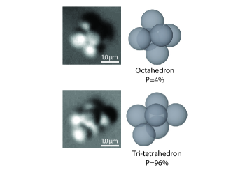
Figure 1: Equilibrium between octahedral and tri-tetrahedral structures. Meng and collaborators experimentally observed the tri-tetrahedron (bottom) 24 times as often as the octahedron (top) Meng et al. (2010). This difference is due primarily to the tri-tetrahedron’s higher rotational entropy.

To understand why the tri-tetrahedron occurs so much more often, Meng and colleagues used a statistical mechanical model originally developed for molecules, in which the total partition function $Q^{\prime}$ is written as the product of partition functions for collective translations, rotations, and vibrations: $Q^{\prime}=Q^{\prime}_{\textnormal{trans}}Q^{\prime}_{\textnormal{rot}}Q^{\prime}_{\textnormal{vib}}$. Each term represents a different entropic contribution to the free energy. Because the partition function is proportional to the probability of observation in equilibrium, the ratio of the partition functions for the tri-tetrahedron and octahedron should be 24:1.

Meng and coworkers found that the largest contribution to the factor of 24 comes from a factor called the symmetry number, which accounts for all the permutations of particles that lead to the same structure. The number of ways in which six particles can form an octahedron, which has multiple axes of fourfold, threefold, and twofold symmetry, is much smaller than the number of ways in which six particles can form the tri-tetrahedron, which has only one axis of twofold symmetry. Thus, the octahedron has a much larger symmetry number than the tri-tetrahedron. In equilibrium, the tri-tetrahedron is therefore favored by a factor of 12, corresponding to the ratio of symmetry numbers. We discuss the origin of the symmetry number and its physical interpretation in more detail in Sections II and III.

The remaining factor of two comes from a term in the rotational partition function that is proportional to the product of the moments of inertia, which differs between the two structures, and the vibrational partition function, which can be calculated using a harmonic approximation for the potential.

The model can be generalized to two-dimensional systems Morgan and Wales (2014); Perry et al. (2015) and to clusters with $N>6$ particles, where the number of minimal-energy structures increases rapidly with $N$ Meng et al. (2010); Perry et al. (2012); Kallus and Holmes-Cerfon (2017). One interesting result from these studies is the dominance of symmetry effects when $N$ is small: Meng and coworkers found that when $N<9$, the clusters always favor asymmetric configurations in equilibrium.

I.2 Overview

In what follows, we explain why the partition function can be written in the form above, and how the factors that appear in the rotational and vibrational parts affect the equilibrium probabilities. To do this, we first introduce the elements and assumptions of our model in Section II.1 and then derive the partition function in two different coordinate systems: particle coordinates (Section II.2) and center-of-mass coordinates (Section II.3). The formulation in particle coordinates does not lend itself to analytical calculations, whereas that in center-of-mass coordinates can be used to explicitly calculate the observation probabilities. However, the derivation in particle coordinates is more general, and we use it to gain physical insights into the terms in the center-of-mass formulation. In the discussion (Section III) we equate the two versions to explain the origin and roles of the symmetry number and the dynamical quantities that appear in the center-of-mass formulation—the moments of inertia and the vibrational frequencies.

II The statistical mechanical model

II.1 Framework

We seek a model for the experimental observable $P_{s_{k}}$, the probability of observing a particular structure $s_{k}$ in an equilibrium ensemble. For example, in the $N=6$ case discussed above, there are two structures: $s_{1}=\textnormal{octahedron}$ and $s_{2}=\textnormal{tri-tetrahedron}$. In equilibrium, $P_{s_{k}}$ is proportional to $Q_{s_{k}}$, the partition function of $s_{k}$:

$$P_{s_{k}}=\frac{Q_{s_{k}}}{\sum_{l}{Q_{s_{l}}}},$$ (1)

where the summation ranges over all structures $s_{l}$ in the ensemble. In experiments, one usually counts only clusters that represent minima in the energy—that is, those with at least $3N-6$ bonds—as part of the ensemble. States with fewer bonds are ignored. We calculate the partition function in the two coordinate systems illustrated in Fig. 2: particle coordinates and center-of-mass coordinates.

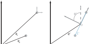
Figure 2: In particle coordinates (left) the positions of every particle ($\mathbf{q}_{i}$) are measured from the origin of a lab frame. In center-of-mass coordinates (right), we define a rotating frame (dark gray) with an origin $O$ at the cluster’s center of mass; the position of $O$ relative to the lab frame is given by $\mathbf{q^{\prime}}$. The rotating frame is chosen to lie along the cluster’s principal axes. The standard Euler angles (the first of which is $\phi^{\prime}$) describe its rotation relative to the lab frame. Within the rotating frame, the coordinates of the vibrational modes are denoted by $\xi^{\prime}$. Particles are also free to rotate about their own centers of mass. Describing these rotations requires another rotating coordinate system located at the center of mass of each particle (light gray axes on left).

II.1.1 Interactions

We assume that our system is at constant temperature and that the interactions between particles are pairwise additive and spherically symmetric. We also assume that the potential is short-ranged. These are good approximations for the experimental systems discussed above: micrometer-scale electrostatically-stabilized particles subject to depletion interactions in water at moderate to high salt concentrations. The repulsions are short-ranged because the salt screens electrostatic interactions. The depletion attraction is short-ranged because the particles that cause it are typically much smaller than the diameter $d$ of the colloidal particles.

II.1.2 Degrees of freedom

We define the phase space of our system by the positional degrees of freedom and their conjugate momenta. We implicitly account for the degrees of freedom of the solvent molecules by using a potential of mean force to describe the interactions between the particles. This potential is a thermal average over all the configurations of solvent molecules Frenkel (2006). Therefore the phase space is determined by the degrees of freedom of the particles alone.

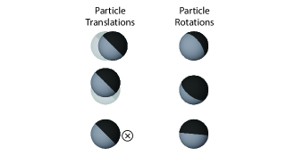
Figure 3: An individual colloidal particle has six positional degrees of freedom: three translational and three rotational. The three translational degrees of freedom have three conjugate linear momenta, and the three rotational degrees of freedom have three conjugate angular momenta. The rotational degrees of freedom might be observed by watching small defects on the surfaces of the particles or by dyeing one hemisphere of each particle, as illustrated here.

To illustrate how the degrees of freedom differ in the two coordinate systems, we consider a dimer. In the particle coordinate system, the dimer has 12 positional degrees of freedom: each particle can translate in each of the three dimensions, and each can rotate about three independent axes centered on its center of mass. The rotational motions can in principle be observed by tracking small defects on the surfaces of the particles or by dyeing part of each particle, as shown in Fig. 3. Interactions such as depletion change the distribution of values for each degree of freedom relative to a gas, but they do not change the number or type of degrees of freedom.

In the center-of-mass coordinate system, the dimer also has 12 degrees of freedom (Fig. 4). Three correspond to translations of the center of mass, two to rotations of the cluster about its center of mass, one to vibrations of the bond, and the remaining six to internal modes. An internal mode is one where particles rotate about their own centers of mass, either in the same direction or in the opposite direction as their partners. The top left internal mode in Fig. 4 (bottom) is equivalent to rotations of the entire dimer about its axis.

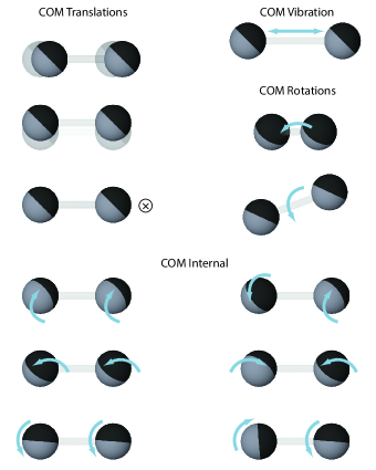
Figure 4: In center-of-mass coordinates, a colloidal dimer has 12 degrees of freedom, three corresponding to full-body translations, two to full body rotations, one to vibration, and six others to internal modes. The internal degrees of freedom arise from the rotations of individual colloidal particles.

Importantly, none of these modes can be “frozen out,” as might happen in a molecular system. In a diatomic molecule such as $N_{2}$, the excited vibrational states are not accessible at room temperature, because the energy levels are much larger than the thermal energy. In the classical dimer, all 12 modes can be excited, and we account for all of them in our derivation. We do, however, neglect modes associated with vibrations of the molecules inside the particles.

II.1.3 Distinguishability

Whereas in a molecule like $N_{2}$, the two nitrogen atoms are fundamentally indistinguishable (if they are the same isotope), in a colloidal system the particles are distinguishable, as discussed above. However, we can choose not to distinguish the particles from one another. This is a common—if not universal—tactic used in the analysis of experiments on colloidal self-assembly Cates and Manoharan (2015). The term undistinguished, coined by Sethna Sethna (2006), describes the particles in this situation. We assume undistinguished particles throughout.

II.2 Partition function in particle coordinates

In particle coordinates, each particle has six positional degrees of freedom (Fig. 3)—three translational and three rotational—and six associated momenta—three linear and three angular. Thus, a cluster of $N$ particles has $6N$ positional degrees of freedom and $6N$ associated momenta.

The translational degrees of freedom for the $i$th particle $(q_{ix},q_{iy},q_{iz})$ are measured as displacements from the origin (Fig. 2, left), which is fixed in the lab frame. The set of all translational degrees of freedom is $\mathbb{Q}=(q_{1x},q_{1y},q_{1z},\ldots,q_{Nz})$. The linear momenta corresponding to the translational degrees of freedom for the $i$th particle are $\mathbf{p}_{i}=(p_{ix},p_{iy},p_{iz})$, and the set of all linear momenta is $\mathbb{P}$.

Each particle can also rotate about its own center of mass. We describe these rotations using a rotating frame with its origin at the particle’s center of mass (light gray axes in Fig. 2, left). Each particle $i$ can rotate through Euler angles $(\phi_{i},\theta_{i},\psi_{i})$ relative to the lab frame. The set of all such angles is $\bm{\Phi}=(\phi_{1},\theta_{1},\psi_{1},\ldots,\phi_{N},\theta_{N},\psi_{N})$. The angular kinetic energy of the individual particles depends on the set of all momenta $\mathbb{L}$ conjugate to the Euler angles.

With the definitions above, we can express the Hamiltonian $\mathcal{H}$ for a system of $N$ particles as

$$\begin{split}\mathcal{H}&=U(\mathbb{Q})+K(\mathbb{P})+U(\bm{\Phi})+K(\mathbb{L}),\end{split}$$ (2)

where $U$ is potential energy—again, a potential of mean force—and $K$ is kinetic energy. The canonical partition function $Q$ is then

$$Q\propto\int{e^{-\beta\mathcal{H}}}d\mathbb{Q}\,d\mathbb{P}\,d\bm{\Phi}\,d\mathbb{L},$$ (3)

where $\beta=1/(k_{B}T)$, $k_{B}$ being Boltzmann’s constant and $T$ the temperature of our system. We use a proportionality symbol because we have yet to determine the bounds and the prefactors.

The bounds on the integral must be consistent with our definition of the structure $s$. If we were to integrate over all of phase space, then the partition function would include all possible structures. Instead, we integrate only over those parts of phase space in which the particles are arranged in a particular structure $s$.

One way to define the structure is through an adjacency matrix $\mathbf{A}_{s}$ Arkus et al. (2009, 2011), a symmetric, $N\times N$ matrix. An element $A_{ij}$ is equal to 1 if particle $i$ is bound to particle $j$, and 0 otherwise. To determine whether two particles are bound, we must first set a cutoff distance $\ell$. For instance, $\ell$ might be the maximum range of the depletion force. For a short-range interaction, $(\ell-d)/d\ll 1$. This definition requires assigning a unique label to each particle in our structure.

We would like the partition function for a structure $s$ to integrate over all fluctuations of that structure, because experiments do not distinguish structures by their center-of-mass positions, orientations, or distances between particles (as long as the center-to-center distance between particles is less than $\ell$). The adjacency matrix $\mathbf{A}_{s}$ is a convenient way to delineate the bounds on phase space because it describes the structure irrespective of such fluctuations. Therefore, if we set the bounds on the integral in Eq. (3) to include the region of phase space in which the adjacency matrix is $\mathbf{A}_{s}$, the partition function will include contributions from the rotations of the individual particles, translations of the entire cluster, rotations of the entire cluster, and fluctuations in interparticle distances.

However, some of these fluctuations correspond to different representations of the same structure. The overlap arises because the adjacency matrix is not a unique representation of a structure. There are $N!$ different adjacency matrices that correspond to the same structure because there are $N!$ permutations of particle labels. Some of these permutations are identical to other permutations plus full-body rotations, as illustrated in Fig. 5. Therefore, for any given representation of the structure (any particular adjacency matrix), we must divide the partition function by a factor that accounts for how many orientations are shared with a different representation. That factor is the symmetry number $\sigma_{s}$. It is equal to 24 for the octahedron, as shown in Fig. 5.

Figure 5: 24 of the 720 colorings, or label permutations, of the octahedron. All of these colorings are equivalent through rotations.

The symmetry number $\sigma_{s}$ accounts for all the ways in which permutations plus rotations yield an identical cluster. We discuss $\sigma_{s}$ in more detail in section III.2. We note here that because $\sigma_{s}$ appears even in our classical derivation, it cannot arise from any quantum mechanical considerations. As noted by Gilson and Irikura Gilson and Irikura (2010), $\sigma_{s}$ is a mathematical artifact arising from how we define the region of phase space that we integrate over. Indeed, it can be calculated from the size of the automorphism group of the adjacency matrix Arkus et al. (2011).

A further complication is that a given adjacency matrix can correspond to chiral enantiomers Arkus et al. (2011) or two or more geometrically-distinct clusters Holmes-Cerfon (2016). Therefore, if we were to integrate over the regions of phase space corresponding to one such matrix, we would include contributions from structures that an experimentalist might treat as different. However, we will not use the partition function in particle coordinates to evaluate the equilibrium probabilities; we use this version only to gain insight into the partition function in center-of-mass coordinates, which is much more tractable. With this aim in mind, we restrict our discussion to only those cases in which the adjacency matrix defines a single structure.

Finally, we must include a prefactor of $1/h^{6N}$ for dimensional consistency, where $h$ is a placeholder for any quantity with dimensions of momentum times length. The exponent of $6N$ arises because there is one factor of $h$ for each conjugate pair of position and momentum in phase space. We do not claim—nor do we need to claim—that $h$ is Planck’s constant, since the quantity $h$ must cancel in the statistical mechanical calculation of any classical observable. It can appear only if a degree of freedom is frozen out, in which case the calculation is no longer classical.

The resulting partition function for a structure $s$ is

$$Q_{s}=\frac{1}{\sigma_{s}h^{6N}}\int_{\mathbf{A}_{s}}{e^{-\beta\mathcal{H}}}d\mathbb{Q}\,d\mathbb{P}\,d\bm{\Phi}\,d\mathbb{L},$$ (4)

where the subscript $\mathbf{A}_{s}$ reminds us that the integral is over the region of phase space corresponding to just one labeling.

The separability of the Hamiltonian in Eq. 2 allows us to factor the partition function into configurational and momentum components:

$$\begin{split}Q_{s}=\frac{1}{\sigma_{s}h^{6N}}&\int_{\mathbf{A}_{s}}{e^{-\beta\mathcal{H}}}d\mathbb{Q}\,d\mathbb{P}\,d\bm{\Phi}\,d\mathbb{L}\\ =\frac{1}{\sigma_{s}h^{6N}}&\int_{\mathbf{A}_{s}}{e^{-\beta U(\mathbb{Q})}}d\mathbb{Q}\int{e^{-\beta K(\mathbb{P})}}d\mathbb{P}\\ &\times\int{e^{-\beta U(\bm{\Phi})}}d\bm{\Phi}\int{e^{-\beta K(\mathbb{L})}}d\mathbb{L}\\ =\frac{1}{\sigma_{s}h^{6N}}&Q_{s,\textnormal{trans}}(\mathbb{Q},\mathbb{P})\,Q_{s,\textnormal{rot}}(\bm{\Phi},\mathbb{L}),\end{split}$$ (5)

where the last line defines the translational ($Q_{s,\textnormal{trans}}$) and rotational ($Q_{s,\textnormal{rot}}$) components of the partition function in particle coordinates. Note that the terms “translational” and “rotational” refer to the degrees of freedom of individual particles, not of the center of mass of the entire cluster. Note also that this decomposition holds for all classical systems, because the positions and the momenta always decouple in the classical Hamiltonian. The adjacency matrix determines the bounds only on the integral over $\mathbb{Q}$. The bounds on the linear-momentum integral extends from $-\infty$ to $+\infty$, and the bounds on the integrals defining $Q_{s,\textnormal{rot}}$ extend over all Euler angles and associated momenta.

II.2.1 Translations and linear momenta

We first examine the part of the partition function corresponding to translations of individual particles. From Eq. (5),

$$Q_{s,\textnormal{trans}}=\int_{\mathbf{A}_{s}}{e^{-\beta U(\mathbb{Q})}}d\mathbb{Q}\int{e^{-\beta K(\mathbb{P})}}d\mathbb{P}.$$ (6)

To understand how the structure affects the first integral, we assign effective volumes to each particle in the cluster. We can think of the first particle as free to wander the entire volume $V$ of the container. The second particle, which is bound to the first, is then constrained to a spherical shell around the first particle with inner radius $d$ and thickness $\ell-d$. The effective volume corresponding to this particle depends on the interaction potential, which weights the different regions of the shell. A third particle would be similarly constrained to an effective volume defined by the other particles, and so on.

We can therefore write the configurational partition function $Z_{s}$ as a product of volumes Herschbach et al. (1959):

$$Z_{s}=\int_{\mathbf{A}_{s}}{e^{-\beta U(\mathbb{Q})}}d\mathbb{Q}=V\prod_{i=2}^{N}V_{s,i},$$ (7)

where $V_{s,i}$ is the effective volume that the $i$th particle is allowed to explore in our structure $s$. Here we have assumed that the volume of the container $V$ is much larger than the volume of a single particle. For certain structures, these effective volumes can be calculated explicitly by transforming the integral in Eq. (7) to internal coordinates Herschbach et al. (1959); Boresch and Karplus (1996).

We then integrate over the momenta. The kinetic energy is that for a non-relativistic classical system:

$$\begin{split}K(\mathbb{P})=\sum_{i=1}^{N}{\frac{1}{2m_{i}}(p_{i_{x}}^{2}+p_{i_{y}}^{2}+p_{i_{z}}^{2})}.\end{split}$$

Thus, the translational part of the partition function in particle coordinates is

$$\begin{split}Q_{s,\textnormal{trans}}&=\int_{\mathbf{A}_{s}}{e^{-\beta U(\mathbb{Q})}}d\mathbb{Q}\int{e^{-\beta K(\mathbb{P})}}d\mathbb{P}\\ &=Z_{s}\int{\exp{\left(-\beta\sum_{i=1}^{N}\frac{p_{i_{x}}^{2}+p_{i_{y}}^{2}+p_{i_{z}}^{2}}{2m_{i}}\right)}}d\mathbb{P}\\ &=Z_{s}\prod_{i=1}^{N}\left({\frac{2\pi m_{i}}{\beta}}\right)^{3/2},\end{split}$$ (8)

where the last line follows from evaluating the Gaussian integrals for each momentum component. We note that because our (non-gravitational) potential does not depend on the particle masses, $Z_{s}$ also does not depend on the masses.

II.2.2 Rotations and angular momenta

Finally, we turn to the rotational component of the partition function. From Eq. (5), this component is

$$Q_{\textnormal{s, rot}}=\int{e^{-\beta U(\bm{\Phi})}}d\bm{\Phi}\int{e^{-\beta K(\mathbb{L})}}d\mathbb{L}.$$

It accounts for the rotation of particles about their own centers of mass.

We assume that the rotational potential energy depends neither on the orientations of the particles nor on their positions in the cluster. Hence we can say $U(\bm{\Phi})=0$. This is a good approximation for spherical colloidal particles subject to depletion interactions, which are isotropic and short-ranged. The rotational kinetic energy of the cluster is the sum of that of the individual particles, and so the rotational component of the partition function is the product of the rotational components of each particle.

Therefore, $Q_{\textnormal{s, rot}}$ is a constant that depends on the number of particles $N$ and their moments of inertia, but not the structure $s$. We therefore drop the subscript $s$ on the rotational part and let $Q_{\textnormal{s, rot}}=Q_{\textnormal{rot}}$. Because $Q_{\textnormal{rot}}$ cancels when we calculate the probability of observing a structure $s$ from Eq. (1), we need not calculate it explicitly.

II.2.3 Complete partition function in particle coordinates

The complete partition function for a structure $s$ in particle coordinates is

$$\begin{split}Q_{s}&=\frac{1}{\sigma_{s}h^{6N}}Q_{s,\textnormal{trans}}Q_{\textnormal{rot}}\\ &=\frac{Q_{\textnormal{rot}}}{\sigma_{s}h^{6N}}Z_{s}\prod_{i=1}^{N}\left({\frac{2\pi m_{i}}{\beta}}\right)^{3/2}\\ &=\frac{Q_{\textnormal{rot}}}{\sigma_{s}h^{6N}}\left(\frac{2\pi}{\beta}\right)^{3N/2}\left(V\prod_{i=2}^{N}V_{i}\right)\prod_{i=1}^{N}m_{i}^{3/2}.\end{split}$$ (9)

The version for quasi-two-dimensional systems is given in the Appendix.

The probability of observing structure $s_{1}$ relative to that of $s_{2}$, where both structures have the same $N$ particles, is

$$\frac{P_{s_{1}}}{P_{s_{2}}}=\frac{Q_{s_{1}}}{Q_{s_{2}}}=\frac{\sigma_{s_{2}}}{\sigma_{s_{1}}}\frac{Z_{s_{1}}}{Z_{s_{2}}}$$ (10)

where $Q_{\textnormal{rot}}$ has canceled because it does not depend on $s$. The ratio of the probabilities is therefore inversely proportional to the ratio of symmetry numbers and directly proportional to the ratio of $Z_{s}$, which is the product of effective volumes.

Equation (10) has a straightforward physical interpretation. Structures with greater flexibility or range of internal motion are favored in equilibrium because they have larger effective volumes or, equivalently, larger $Z_{s}$. As we discuss below, $Z_{s}$ is related to vibrations and rotations in center-of-mass coordinates. Equation (10) also shows that structures with low symmetry are favored over those with high symmetry. We discuss this effect in Section III.2.

Lastly, we note that the masses of the individual particles, even if different, have no effect on the ratio of equilibrium probabilities, as long as the total masses of the clusters are the same. The masses cancel from the probability ratio under the assumptions we have made.

II.3 Partition function in center-of-mass coordinates

Calculation of the equilibrium probabilities is simpler in the center-of-mass coordinate system because we can make the rigid-rotor-harmonic-oscillator approximation. Below, we explain and justify this approximation and then derive the partition function. We use a prime (^′) symbol to denote all quantities defined in center-of-mass coordinates.

The rigid-rotor-harmonic-oscillator approximation allows us to separate the Hamiltonian into terms that describe the translation of the center of mass, rotations about the center of mass, and vibrations of particles about their lowest-energy (equilibrium) positions Wilson et al. (1980). For this approximation to hold, the amplitude of the vibrational motion must be small compared to the equilibrium distance between particle centers. In that case, we can treat the rotations of the cluster using rigid-body mechanics and the vibrations using a normal-mode framework.

We justify this approximation on three grounds. First, we expect the vibrational motion to be small because the interactions are short-ranged for a typical colloidal system. Second, Meng and coworkers Meng et al. (2010, 2014) showed that a harmonic potential is a reasonable approximation for the combination of a depletion interaction and electrostatic repulsion. Third, and most importantly, Meng and colleagues showed that the predictions of a statistical mechanical model based on the rigid-rotor-harmonic-oscillator approximation gave excellent agreement with experiment.

In applying this approximation, we must limit our analysis to those clusters that rotate as rigid bodies. We therefore exclude “singular” clusters, which are minima of the potential energy containing at least $3N-6$ pair interactions but which contain zero-frequency vibrational modes. Kallus and Holmes-Cerfon have shown how to calculate the free energy for these clusters Kallus and Holmes-Cerfon (2017). We also exclude hyperstatic clusters—those with more than $3N-6$ pair interactions. We restrict the derivation to non-singular isostatic clusters ($3N-6$ pair interactions with no zero-frequency modes) because our primary goal is to give physical insight into the form of the partition function.

We can describe a non-singular, non-hyperstatic cluster of $N$ particles in center-of-mass coordinates using three translational, three rotational, $3N-6$ vibrational, and $3N$ internal degrees of freedom. As in particle coordinates, there are a total of $6N$ positional degrees of freedom and $6N$ associated momenta. However, each positional degree of freedom now describes a collective motion of all the particles in the cluster.

We define our coordinate system as follows. There is a lab frame with a fixed origin and a rotating frame with an origin $O$ at the center of mass of our cluster (Fig. 2, right). We choose the rotating frame such that the axes lie along the principal axes of the cluster. For symmetric clusters, there may be more than one choice of principal axes; we arbitrarily pick one set.

Six degrees of freedom describe the position and orientation of the rotating frame relative to the lab frame. The translational degrees of freedom $\mathbf{q}^{\prime}=(q_{x}^{\prime},q_{y}^{\prime},q_{z}^{\prime})$ describe the position of $O$ relative to the lab origin. Their conjugate linear momenta are $\mathbf{p}^{\prime}=(p_{x}^{\prime},p_{y}^{\prime},p_{z}^{\prime})$. The rotational degrees of freedom $\bm{\Phi}^{\prime}=(\phi^{\prime},\theta^{\prime},\psi^{\prime})$ are the standard Euler angles. Their conjugate angular momenta are $\mathbb{L}^{\prime}=(p_{\phi}^{\prime},p_{\theta}^{\prime},p_{\psi}^{\prime})$.

With the harmonic approximation, we can describe the vibrations of the cluster using a set of $3N-6$ orthogonal harmonic modes. The displacement along the $j$th mode is $\xi^{\prime}_{j}$, and the set of all vibrational displacements is $\bm{\xi}^{\prime}=(\xi^{\prime}_{1},\ldots,\xi^{\prime}_{3N-6})$. When all the particles are in their lowest potential-energy configurations, $\bm{\xi}^{\prime}=0$. The momentum conjugate to the vibrational coordinate for the $j$th mode is $\chi^{\prime}_{j}$, and the set of all vibrational momenta is $\bm{\chi}^{\prime}$.

Under these assumptions the Hamiltonian in center-of-mass coordinates becomes

$$\begin{split}\mathcal{H}_{s}^{\prime}&=\mathcal{H}_{s,\textnormal{trans}}^{\prime}+\mathcal{H}_{s,\textnormal{rot}}^{\prime}+\mathcal{H}_{s,\textnormal{vib}}^{\prime}+\mathcal{H}_{\textnormal{rot}}\\ &=U_{s}(\mathbf{q}^{\prime})+K_{s}(\mathbf{p}^{\prime})+U_{s}(\bm{\Phi}^{\prime})+K_{s}(\mathbb{L}^{\prime})\\ &\quad+U_{s}(\bm{\xi}^{\prime})+K_{s}(\bm{\chi}^{\prime})+\mathcal{H}_{\textnormal{rot}}(\bm{\Phi},\mathbb{L}),\end{split}$$ (11)

where, for completeness, we have included a term describing the rotations of individual particles. The partition function $Q_{s}^{\prime}$ is then

$$\begin{split}Q_{s}^{\prime}=\frac{1}{\sigma_{s}h^{6N}}&\int{e^{-\beta\mathcal{H}_{s}^{\prime}}}d\mathbf{q}^{\prime}\,d\mathbf{p}^{\prime}\,d\bm{\Phi}^{\prime}\,d\mathbb{L}^{\prime}\,d\bm{\xi}^{\prime}\,d\bm{\chi}^{\prime}\,d\bm{\Phi}\,d\mathbb{L}\\ =\frac{Q_{\textnormal{rot}}}{\sigma_{s}h^{6N}}&\int{e^{-\beta\mathcal{H}^{\prime}_{\textnormal{trans}}}}\,d\mathbf{q}^{\prime}\,d\mathbf{p}^{\prime}\int{e^{-\beta\mathcal{H}^{\prime}_{\textnormal{rot}}}}\,d\bm{\Phi}^{\prime}\,d\mathbb{L}^{\prime}\\ &\times\int{e^{-\beta\mathcal{H}^{\prime}_{\textnormal{vib}}}}\,d\bm{\xi}^{\prime}\,d\bm{\chi}^{\prime}\\ =\frac{Q_{\textnormal{rot}}}{\sigma_{s}h^{6N}}&Q_{s,\textnormal{trans}}^{\prime}(\mathbf{q}^{\prime},\mathbf{p}^{\prime})Q_{s,\textnormal{rot}}^{\prime}(\bm{\Phi}^{\prime},\mathbb{L}^{\prime})Q_{s,\textnormal{vib}}^{\prime}(\bm{\xi}^{\prime},\bm{\chi}^{\prime}),\end{split}$$ (12)

where the last line defines the translational ($Q_{s,\textnormal{trans}}^{\prime}$), rotational ($Q_{s,\textnormal{rot}}^{\prime}$), and vibrational ($Q_{s,\textnormal{vib}}^{\prime}$) partition functions in center-of-mass coordinates. As we did in particle coordinates, we express the contribution of individual particle rotations as $Q_{\textnormal{rot}}$, which is a constant for all structures formed from the same $N$ particles. We also divide by the symmetry number $\sigma_{s}$ to avoid overcounting rotational states. We discuss the role of the symmetry number in more detail in Section III.2.

The expression for the partition function in Eq. (12) is more tractable than the one in particle coordinates [Eq. (9)] because we need not set any cutoff distances that depend on the structure. Instead, we can integrate over all possible values of the translational, rotational, and vibrational coordinates.

The absence of bounds that depend on the structure raises the question of where exactly we specify the structure when we calculate the integral. The structure is in fact encoded in how the coordinates couple to the energies. For example, different structures have different harmonic modes, and these modes couple to the vibrational energy through a set of natural frequencies that are different for each structure. Furthermore, although the rotational modes of all the clusters are the same—they represent rotations about three orthogonal axes—these modes couple to the angular kinetic energy through the principal moments of inertia, which differ from structure to structure. Below, we analytically integrate the translational, rotational, and vibrational partition functions and point out the terms that define the structure.

II.3.1 Center-of-mass translations and linear momenta

We start by calculating the translational partition function in Eq. (12), which is given by

$$Q_{s,\textnormal{trans}}^{\prime}=\int e^{-\beta U^{\prime}_{s}(\mathbf{q}^{\prime})}d\mathbf{q}^{\prime}\int e^{-\beta K^{\prime}_{s}(\mathbf{p}^{\prime})}d\mathbf{p}^{\prime}.$$

We assume that the potential energy of the cluster does not vary with its position in space, such that $U^{\prime}(\mathbf{q}^{\prime})=0$.

The first integral in the translational partition function is then equal to the volume available to the cluster, which is the total volume $V$ of the container less any volume that the cluster cannot access without penetrating a boundary. We can neglect this excluded volume if $V\gg V_{s}$, where $V_{s}$ is some measure of the volume of a particular structure. With this approximation,

$$\int e^{-\beta U^{\prime}(\mathbf{q}^{\prime})}d\mathbf{q}^{\prime}=V.$$

The second integral in the translational partition function can also be analytically integrated. The translational kinetic energy of the center of mass of the cluster is given by

$$K^{\prime}(\mathbf{p}^{\prime})=\frac{1}{2M}(p_{x}^{\prime 2}+p_{y}^{\prime 2}+p_{z}^{\prime 2}),$$

where $M=\sum_{i=1}^{N}{m_{i}}$ is the total mass of the cluster. After evaluating the resulting Gaussian integral, we find that

$$\begin{split}Q_{\textnormal{s, trans}}^{\prime}&=V\left({\frac{2\pi M}{\beta}}\right)^{3/2}.\end{split}$$

II.3.2 Center-of-mass rotations and angular momenta

The rotational partition function in center-of-mass coordinates describes the free rotation of the cluster about its center of mass:

$$Q_{s,\textnormal{rot}}^{\prime}=\int e^{-\beta U^{\prime}_{s}(\bm{\Phi}^{\prime})}d\bm{\Phi}^{\prime}\int e^{-\beta K^{\prime}_{s}(\mathbb{L}^{\prime})}d\mathbb{L}^{\prime}.$$ (13)

We assume that the potential energy of the cluster is independent of its orientation, such that $U^{\prime}(\bm{\Phi}^{\prime})=0$. We need not include a Jacobian term when the rotational partition function is written in the form above, which is an integral over the the Euler angles $\bm{\Phi}^{\prime}=(\phi^{\prime},\theta^{\prime},\psi^{\prime})$ and their conjugate angular momenta $\mathbb{L}^{\prime}$.

However, it is more natural to express the second integral in Eq. (13) in terms of the angular velocities $\bm{\Omega}^{\prime}$ of the cluster about its principal axes:

$$\begin{split}&\Omega_{1}^{\prime}=\dot{\theta}^{\prime}\sin{\psi^{\prime}}-\dot{\phi}^{\prime}\sin{\theta^{\prime}}\cos{\psi^{\prime}}\\ &\Omega_{2}^{\prime}=\dot{\theta}^{\prime}\cos{\psi^{\prime}}+\dot{\phi^{\prime}}\sin{\theta^{\prime}}\sin{\psi^{\prime}}\\ &\Omega_{3}^{\prime}=\dot{\psi}^{\prime}+\dot{\phi^{\prime}}\cos{\theta^{\prime}},\end{split}$$

where the dots denote time derivatives, and the subscripts denote principal axes. The angular kinetic energy of the cluster is then

$$K^{\prime}_{s}(\bm{\Omega}^{\prime})=\frac{1}{2}\left(I_{s,1}\Omega_{1}^{\prime 2}+I_{s,2}\Omega_{2}^{\prime 2}+I_{s,3}\Omega_{3}^{\prime 2}\right),$$ (14)

where $I_{s,1}$, $I_{s,2}$, and $I_{s,3}$ are the principal moments of inertia, which depend on the specific structure $s$.

Following A. Wilson Wilson (1957), we change variables from the conjugate momenta $(p_{\theta}^{\prime},p_{\phi}^{\prime},p_{\psi}^{\prime})$ to the angular velocities $(\Omega_{1}^{\prime},\Omega_{2}^{\prime},\Omega_{3}^{\prime})$. We calculate the momenta from derivatives of the Lagrangian $\mathcal{L}^{\prime}=K^{\prime}-U^{\prime}$ with $U^{\prime}=0$ as discussed above:

$$\begin{split}p_{\theta}^{\prime}=\frac{\partial{K_{s}^{\prime}}}{\partial{\dot{\theta}^{\prime}}}&=I_{s,1}\Omega_{1}^{\prime}\sin{\psi^{\prime}}+I_{s,2}\Omega_{2}^{\prime}\cos{\psi^{\prime}}\\ p_{\phi}^{\prime}=\frac{\partial{K_{s}^{\prime}}}{\partial{\dot{\phi}^{\prime}}}&=-I_{s,1}\Omega_{1}^{\prime}\sin{\theta^{\prime}}\cos{\psi^{\prime}}\\ &\quad+I_{s,2}\Omega_{2}^{\prime}\sin{\theta^{\prime}}\sin{\psi^{\prime}}+I_{s,3}\Omega_{3}^{\prime}\cos{\theta^{\prime}}\\ p_{\psi}^{\prime}=\frac{\partial{K_{s}^{\prime}}}{\partial{\dot{\psi}^{\prime}}}&=I_{s,3}\Omega_{3}^{\prime}.\end{split}$$ (15)

The change of variables introduces a Jacobian term

$$J=\frac{\partial\left(p_{\theta}^{\prime},p_{\phi}^{\prime},p_{\psi}^{\prime}\right)}{\partial\left(\Omega_{1}^{\prime},\Omega_{2}^{\prime},\Omega_{3}^{\prime}\right)}=I_{s,1}I_{s,2}I_{s,3}\sin{\theta^{\prime}}.$$

We can then integrate to yield the rotational partition function:

$$\begin{split}Q_{s,\textnormal{rot}}^{\prime}=&\int e^{-\beta U_{s}(\bm{\Phi}^{\prime})}d\bm{\Phi}^{\prime}\int e^{-\beta K_{s}(\mathbb{L}^{\prime})}d\mathbb{L}^{\prime}\\ =&\iint Je^{-\beta U_{s}(\bm{\Phi}^{\prime})}e^{-\beta K_{s}(\bm{\Omega}^{\prime})}d\bm{\Phi}^{\prime}\,d\bm{\Omega}^{\prime}\\ =&\,I_{s,1}I_{s,2}I_{s,3}\int\sin{\theta^{\prime}}\,d\bm{\Phi}^{\prime}\\ &\times\int{\exp{\left[-\frac{\beta}{2}\left(I_{s,1}\Omega_{1}^{\prime 2}+I_{s,2}\Omega_{2}^{\prime 2}+I_{s,3}\Omega_{3}^{\prime 2}\right)\right]}}d\bm{\Omega}^{\prime}\\ =&\,8\pi^{2}\left(\frac{2\pi}{\beta}\right)^{3/2}\sqrt{I_{s,1}I_{s,2}I_{s,3}},\end{split}$$ (16)

II.3.3 Vibrational modes

Finally, we calculate the partition function associated with the remaining $3N-6$ degrees of freedom. The vibrational partition function is given by

$$Q_{s,\textnormal{vib}}^{\prime}=\int e^{-\beta U^{\prime}_{s}(\bm{\xi}^{\prime})}d\bm{\xi}^{\prime}\int e^{-\beta K^{\prime}_{s}(\bm{\chi}^{\prime})}d\bm{\chi}^{\prime}.$$

The harmonic modes that we use to describe the vibrations are the eigenvectors of the mass-weighted Hessian (where the $ik$th entry is scaled by $1/\sqrt{m_{i}m_{k}}$). We select only the $3N-6$ modes that have non-zero eigenvalues. The $j$th eigenvector has an associated eigenvalue that we denote $\omega_{j}$. Thus, the vibrational potential energy can be expressed as a product of squared displacements along the modes:

$$\begin{split}U_{s}^{\prime}(\bm{\xi}^{\prime})=U_{0}+\sum_{j=1}^{3N-6}{\frac{\omega^{2}_{s,j}}{2}\xi_{j}^{\prime 2}},\end{split}$$

where $\xi_{j}^{\prime}$ is the displacement along the $j$th mode and $U_{0}$ is the total potential energy in the absence of vibrational excitations. We set $U_{0}=0$ from here on.

The vibrational kinetic energy is

$$K_{s}^{\prime}(\bm{\chi}^{\prime})=\sum_{j=1}^{3N-6}\frac{1}{2}\chi_{j}^{\prime 2},$$

where $\chi_{j}$ is the (mass-weighted) momentum along the $j$th mode.

We can then analytically integrate the vibrational partition function to obtain

$$\begin{split}Q_{s,\textnormal{vib}}^{\prime}=&\int{\exp{\left(-\frac{\beta}{2}\sum_{j=1}^{3N-6}{\omega^{2}_{s,j}\xi_{j}^{\prime 2}}\right)}}d\bm{\xi}^{\prime}\\ &\times\int\exp\left(-\frac{\beta}{2}\sum_{j=1}^{3N-6}\chi_{j}^{\prime 2}\right)d\bm{\chi}^{\prime}\\ =&\prod_{j=1}^{3N-6}\frac{2\pi}{\beta\omega_{s,j}}.\end{split}$$

II.3.4 Complete partition function in center-of-mass coordinates

Putting together the translation, rotational, and vibrational components with the prefactor in Eq. (12), we obtain the complete partition function of a structure $s$ in center-of-mass coordinates:

$$Q_{s}^{\prime}=\frac{Q_{\textnormal{rot}}}{\sigma_{s}h^{6N}}{8\pi^{2}VM^{3/2}}\left({\frac{2\pi}{\beta}}\right)^{3N-3}\sqrt{I_{s,1}I_{s,2}I_{s,3}}\left(\prod_{j=1}^{3N-6}\frac{1}{\omega_{j}}\right)$$ (17)

The version for quasi-two-dimensional systems is given in the Appendix. We note that $Q_{\textnormal{rot}}$, which accounts for the rotations of individual particles, will cancel in the calculation of the cluster probabilities. Apart from the factor of $Q_{\textnormal{rot}}/h^{3N}$, Eq. (17) is equivalent to the molecular partition function, in that the same expression can be derived from the quantum version of the Hamiltonian by taking the high-temperature limit. In this limit, no modes are frozen out.

It is much easier to calculate an explicit value of the partition function with the center-of-mass formulation, Equation (17), than with the particle coordinate formulation, Eq. (9). Apart from $Q_{\textnormal{rot}}$, all the constants in Eq. (17)—the moments of inertia, the vibrational frequencies, and the total mass—can be calculated directly from the positions and masses of the particles. By contrast, in Eq. (9), we must calculate the volumes associated with all fluctuations of the structure. Calculating these effective volumes requires calculating a Jacobian for each particle Herschbach et al. (1959); Boresch and Karplus (1996), because the momenta are already integrated out. By using the rigid-rotor-harmonic-oscillator approximation and taking advantage of the separability of translations, rotations, and vibrations, we are largely able to avoid the calculations of Jacobians in Eq. (17). In the vibrational partition function, for example, we use a coordinate system natural to the vibrational modes (and different from that for the rotational modes) and pair the positions along the modes with their conjugate momenta.

However, this separability comes at a cost. Certainly it sacrifices generality: Equation (9) does not rely on the rigid-rotor-harmonic-oscillator approximation, whereas Eq. (17) does. The results of experiments do agree with the predictions of Eq. (17), establishing the validity of the approximation. But the more serious problem with Eq. (17) is that it obscures the essential physics. It is written in terms of moments of inertia and vibrational frequencies—dynamical parameters whose names suggest that inertia and vibrations can affect the equilibrium probability. As we discuss below, the terminology associated with these quantities can lead to confusion.

III Discussion

III.1 Moments of inertia and vibrational frequencies

Equation (17) might seem to suggest that the value of the partition function would differ if we switched the location of a massive particle with that of a lighter one in the same structure. Say we have a structure $s$ and a set of particles, all of which have the same sizes and interactions, but one of which is much denser than the others. A cluster with the denser particle located near the center of mass will have much lower moments of inertia than a cluster with the particle located further away, as shown in Fig. 6. Therefore the value of the rotational partition function [Eq. (16)] will be much smaller when the particle is closer to the center of mass. We might then expect that in equilibrium, such a configuration would occur less often than a configuration with the particle further from the center of mass. This behavior is counterintuitive, because we expect inertia to have no effect in a typical colloidal suspension, where the surrounding liquid damps the motion Cates (2012).

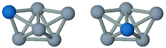
Figure 6: Schematic of a tri-tetrahedral cluster with one particle (blue) that is heavier than the others, but otherwise identical. In this rendering, the pair interactions, or bonds, are shown as struts connecting the particles, which are not drawn to scale. Although the moment of inertia decreases if the particle moves from the position shown on the left to that shown on the right, the equilibrium probability of the cluster does not change, as discussed in the text.

This apparent dependence on the location of the masses is an artifact of the separation of the Hamiltonian into rotational and vibrational components. In particle coordinates, where we do not separate the Hamiltonian, the value of the partition function clearly does not depend on the location of the particles: Equation (9) shows that only the product of the masses matters. Thus, any changes to the moments of inertia resulting from switching the masses must be compensated by changes in the vibrational frequencies.

We can demonstrate this invariance to the positions of the masses by equating the partition function in center-of-mass coordinates, Eq. (17), to that in particle coordinates, Eq. (9). The value of the partition function for a given structure $s$ should be the same in both coordinate systems if the rigid-rotor-harmonic-oscillator approximation is valid. Several terms cancel when we equate the two, including $Q_{\textnormal{rot}}$, $\sigma_{s}$, and $h$.

The remaining terms can be sorted into two groups: those that depend on the particle masses, and those that do not. The terms that depend on the masses are the sum of masses $M$, the product of the moments of inertia $I_{s,1}I_{s,2}I_{s,3}$, and the product of the vibration frequencies $\prod_{j=1}^{3N-6}\omega_{j}$. Terms that do not depend on the masses include the volume $V$, the inverse thermal energy $\beta$, and the configurational partition function $Z_{s}$, which, for a non-gravitational potential, depends only on the interactions and the positions of the particles and not their masses. We can further group the terms that depend implicitly on the masses—the moments of inertia and the vibrational frequencies—on one side of the equation, and the terms that depend explicitly on the masses—$M$ and $\prod_{i=1}^{N}m_{i}$—on the other Perry (2015). We then find:

$$\begin{split}&f(V,\beta,Z_{s})\sqrt{I_{s,1}I_{s,2}I_{s,3}}\left(\prod_{j=1}^{3N-6}\frac{1}{\omega_{j}}\right)=\frac{\prod_{i=1}^{N}m_{i}^{3/2}}{M^{3/2}}\end{split}$$ (18)

where $f(V,\beta,Z_{s})$ is a function that depends neither implicitly nor explicitly on the masses. The form of Eq. (18) agrees with that derived by Herschbach, Johnston, and Rapp Herschbach et al. (1959).

We have therefore shown that the product of the moments of inertia and the inverse vibrational frequencies is proportional to the ratio of a product and a sum of the masses:

$$\sqrt{I_{s,1}I_{s,2}I_{s,3}}\left(\prod_{j=1}^{3N-6}\frac{1}{\omega_{j}}\right)\propto\frac{\prod_{i=1}^{N}m_{i}^{3/2}}{\left(\sum_{i=1}^{N}m_{i}\right)^{3/2}},$$ (19)

Because the products and sums on the right side are invariant to permutations, the product on the left side must also be invariant to the positions of the masses, so long as the structure remains the same.

The discussion above shows that we should consider the moments of inertia as geometrical or structural quantities rather than dynamical ones, at least for the purposes of calculating the partition function. A moment of inertia characterizes the geometrical extent of a cluster—the larger the moment, the larger the radius of gyration of the cluster, and the larger the effective volumes it would sweep out in particle coordinates [Eq. (9)]. Larger moments of inertia correspond to higher entropy.

We also interpret the vibrational frequencies as structural rather than dynamical quantities. Their appearance in the partition function does not mean that the particles actually oscillate. The $\omega_{j}$ appear as a shorthand for the non-zero eigenvalues of the mass-weighted Hessian, and, as such, account for how the structure determines the vibrational potential energy.

III.2 Symmetry

As discussed in Section I.1, structures with low symmetry are favored in equilibrium when $N<9$. This result is exactly as predicted by the statistical mechanical model above: the partition function in either particle or center-of-mass coordinates is inversely proportional to the symmetry number. As a consequence, we expect that in an equilibrium ensemble, structures with lower symmetry occur more often than those with higher symmetry.

To understand why the symmetry number $\sigma_{s}$ appears in the partition function, we must consider how experimentalists measure the equilibrium probabilities. Meng and coworkers Meng et al. (2010) made an equilibrium ensemble of clusters and, using a microscope, took videos of each cluster as it rotated and translated owing to Brownian motion. They identified the structure of each cluster from the videos by visual inspection in the case of the octahedron and tri-tetrahedron, or by determining the networks of contacts and the adjacency matrix in the case of more complicated structures. In either case, they did not distinguish the particles. Finally, to obtain the equilibrium probabilities, they counted the number of times each different structure appeared in the ensemble for a given number of particles.

For a statistical mechanical model to reproduce the experimentally measured probabilities, it must “count” clusters in a similar way—independently of their orientation. An example of a model that does not fit this criterion is one in which we define the bounds on the partition function to include only one particular orientation of a structure. For example, we might include only the orientation of the octahedron with a triangular face facing toward us and a vertex of that face pointing down, as shown in Fig. 5. There are 24 ways in which an octahedral cluster can attain this orientation, owing to its symmetry. We illustrate the 24 different ways by giving different colors to the particles in Fig. 5. By contrast, the same accounting for a tri-tetrahedron would show that there are only two ways of obtaining the same orientation. Thus, our faulty partition function would overcount the octahedron by a factor of $12=24/2$.

To correct our faulty model, we might integrate over all orientations. But in doing so, we must correct for the overcounting of states at any particular orientation. Put another way: the rotational partition function in center-of-mass coordinates, Eq. (16), extends over all Euler angles. But for a given set of principal axes, there are 24 equivalent choices of Euler angles for any orientation of the octahedral cluster. This factor of 24 is the symmetry number $\sigma_{s}$ that we include in the denominator of the partition function, as shown in Eq. (17). As a result, our corrected model predicts that the equilibrium probability of the octahedron relative to the tri-tetrahedron is proportional to $\sigma_{\textnormal{tri-tetrahedron}}/\sigma_{\textnormal{octahedron}}$.

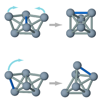
Figure 7: Detailed balance argument for how symmetry affects probability. Top: There is only one bond in the tri-tetrahedron (blue bond in top left) that, once broken, allows the structure to transition to the octahedron. By contrast, breaking any of the 12 symmetrically-equivalent bonds in the octahedron allows it to transition back to the tri-tetrahedron. Bottom: Breaking any other bond in the tri-tetrahedron, such as the blue bond shown, leads back to the tri-tetrahedron.

The argument above explains the mathematical reason for the symmetry number, but it does not explain its apparent physical effect—suppressing the occurrence of highly symmetric clusters like the octahedron. This effect is most easily explained using detailed balance. Let us neglect any fluctuations in bond distances and consider only the ways in which bonds can break. There are 12 symmetrically equivalent bonds in the octahedron, and breaking any of them allows the octahedron to transition to the tri-tetrahedron. By contrast, there is only one bond that, once broken, allows the tri-tetrahedron to transition back to the octahedron, as shown in Fig. 7. Detailed balance then requires that the equilibrium probability of the tri-tetrahedron be a factor of 12 higher than that of the octahedron. This factor is exactly the ratio of symmetry numbers.

To account for the factor of 24 measured in the experiments, we must include contributions from the rotational and vibrational partition functions as well. But the above arguments show clearly that the symmetry number accounts for an entropic effect: there are more ways to arrange particles into a low-symmetry structure like a tri-tetrahedron than a high-symmetry one like the octahedron.

The symmetry number therefore does not account for whether the particles are fundamentally distinguishable or not. Nor does its origin lie in quantum mechanics. It arises because different orientations of a cluster are not counted as different states in the experiment.

IV Conclusions and more questions

We have shown that for isostatic clusters composed of undistinguished particles with a harmonic potential, the partition function for colloidal systems is equivalent to the high-temperature limit of the molecular partition function. We have also shown that the effects of all of its terms on the equilibrium cluster probabilities can be explained classically. By equating the partition functions in particle and center-of-mass coordinates, we have shown that the moments of inertia and vibrational frequencies should be interpreted as geometrical or structural quantities rather than dynamical ones, at least for the purposes of calculating the equilibrium probabilities. We have underscored this point by showing that the ostensible dependence on the positions of the masses in center-of-mass coordinates is an artifact of the separation between rotational and vibrational modes.

The model we derive can be applied to other systems if we relax some of our assumptions. For example, it can be applied to clusters of anisotropic particles Hong et al. (2008); Chen et al. (2011) in which one does distinguish clusters by the orientations of particles within them. In such systems, there is a rotational potential energy term that causes particles to favor certain orientations over others. Thus the $Q_{\textnormal{rot}}$ term will depend on the structure and will not cancel in the observation probabilities.

If we relax the rigid-rotor-harmonic-oscillator approximation, we can begin to describe even more classical systems. For all non-relativistic classical systems with a non-gravitational potential, the form of the partition function in particle coordinates remains the same as what we have derived—so long as it makes sense to define the structure in terms of an adjacency matrix. Thus, for all non-gravitational, non-relativistic classical systems where this structural description is valid, the masses and the positions decouple in the partition function.

Finally, we note that although we have focused on isostatic, rigid colloidal clusters, the singular and hyperstatic clusters are important to understand because they can occur with high probabilities in experiments Meng et al. (2010)—singular clusters because of their high vibrational entropy and hyperstatic clusters because of their low potential energy. The center-of-mass partition function we derive here breaks down in these cases. However, the form of the partition function in particle coordinates is still valid. Kallus and Holmes-Cerfon have developed a theoretical framework to calculate the equilibrium probabilities of such structures Kallus and Holmes-Cerfon (2017).

The overriding goal of both statistical mechanical models and experiments on colloidal clusters of spheres is to understand how the free-energy landscape changes as a function of the number of particles $N$. The landscape quantifies the frustration of the system and how that frustration evolves in the limit as $N\to\infty$, where we expect that the ground state is a crystal. To this end, our model and the physical interpretations we give are important because they give insights into the depths of the minima on the landscape. Although the vibrational framework we use breaks down for non-rigid clusters, the invariance to the positions of masses as well as the entropic effects of the moments of inertia and symmetry number are valid for all clusters. Understanding their physical effects is crucial to making sense of the complex landscape that emerges as $N$ increases.

*

Appendix A Partition function in two dimensions

Here we show the result for the partition function for a two-dimensional (2D) cluster, which differs from the three-dimensional (3D) result because the degrees of freedom are different in two dimensions. While true 2D colloidal systems do not exist, we can model experiments in which 3D spherical particles are confined to a 2D surface. For example, under depletion interactions, planar clusters of spherical particles can form at a surface such as a microscope coverglass Perry et al. (2015). As in three dimensions, the depletion interaction does not prevent the particles in such a quasi-2D cluster from rotating about their centers of mass. However, the collective motions of the cluster are constrained to the plane defined by the surface. Our 2D partition function is specific to such systems.

In particle coordinates, each particle has two positional degrees of freedom. The partition function for a structure $s$ confined to a plane is given by

$$\begin{split}Q_{s}^{2D}&=\frac{Q_{\textnormal{rot}}}{\sigma_{s}^{2D}h^{5N}}\left(\frac{2\pi}{\beta}\right)^{N}Z_{s}^{2D}\prod_{i=1}^{N}m_{i}\\ &=\frac{Q_{\textnormal{rot}}}{\sigma_{s}^{2D}h^{5N}}\left(\frac{2\pi}{\beta}\right)^{N}\left(A\prod_{i=2}^{N}A_{i}\right)\prod_{i=1}^{N}m_{i},\end{split}$$ (20)

where in the second line we have replaced $Z_{s}^{2D}$ by a product of areas for each particle, analogous to the product of volumes in Eq. (9). The factor of $Q_{rot}$ is the same as that in the 3D case because our particles are still free to rotate about their own centers of mass in all three dimensions. The particle rotations also contribute a factor of $1/h^{3N}$ to the partition function, with the remaining factor of $1/h^{2N}$ coming from the translations of individual particles. The symmetry number $\sigma_{s}^{2D}$ differs from that in three dimensions because it does not account for out-of-plane rotations.

In center-of-mass coordinates, the colloidal cluster has two translational degrees of freedom and only one rotational degree of freedom, since the only allowed rotations are in the plane. An isostatic cluster has $2N-3$ vibrational modes. The center-of-mass partition function for a 2D cluster is then

$$Q_{s}^{\prime 2D}=\frac{Q_{\textnormal{rot}}}{\sigma_{s}^{2D}h^{5N}}2\pi AM\sqrt{I_{s}}\left({\frac{2\pi}{\beta}}\right)^{(4N-3)/2}\left(\prod_{j=1}^{2N-3}\frac{1}{\omega_{j}}\right).$$ (21)