Evolution of highly eccentric binary neutron stars including tidal effects

Abstract

This work is the first in a series of studies aimed at understanding the dynamics of highly eccentric binary neutron stars, and constructing an appropriate gravitational-waveform model for detection. Such binaries are possible sources for ground-based gravitational wave detectors, and are expected to form through dynamical scattering and multi-body interactions in globular clusters and galactic nuclei. In contrast to black holes, oscillations of neutron stars are generically excited by tidal effects after close pericenter passage. Depending on the equation of state, this can enhance the loss of orbital energy by up to tens of percent over that radiated away by gravitational waves during an orbit. Under the same interaction mechanism, part of the orbital angular momentum is also transferred to the star. We calculate the impact of the neutron star oscillations on the orbital evolution of such systems, and compare these results to full numerical simulations. Utilizing a Post-Newtonian flux description we propose a preliminary model to predict the timing of different pericenter passages. A refined version of this model (taking into account Post-Newtonian corrections to the tidal coupling and the oscillations of the stars) may serve as a waveform model for such highly eccentric systems.

I Introduction

The LIGO (Laser Interferometric Gravitational Wave Observatory) and Virgo collaborations have already detected five binary black hole (BH) coalescence events Abbott et al. (2016a, b, 2017a, 2017b, 2017c) and one binary neutron star (NS) event Abbott et al. (2017d). Current event rates indicate that as LIGO and Virgo reach design sensitivity in the next few years, many more binary NS coalescences will be observed Abbott et al. (2017d). The formation of binary compact object (CO) systems can be broadly classified into two main categories: field binaries and dynamically assembled (cluster) binaries. In the first channel, the progenitor is a stellar binary where both stars eventually form COs following stellar collapse (with or without supernovae). Such a binary may gain a sizable amount of eccentricity through a supernovae kick, however subsequent gravitational wave (GW) emission will reduce the eccentricity with time, leading to a nearly circular orbit by the time the emission enters the LIGO band. In the second channel, CO binaries form through various N-body interactions that take place in dense stellar environments, including dynamical capture O’Leary et al. (2009); Lee et al. (2010); Kocsis and Levin (2012); Fabian et al. (1975); Pooley et al. (2003), and exchange interactions during binary-single and binary-binary interactionsSamsing et al. (2014); Rodriguez et al. (2015); Samsing (2017).

An exciting aspect of dynamically assembled binaries is that some fraction of these systems will emit GWs in the LIGO/Virgo bands while their orbits are highly eccentric (for order-of-magnitude estimates of these fractions see e.g. East et al. (2013); Samsing et al. (2014); Samsing (2017)). A further mechanism that can produce eccentric mergers within ground-based GW detector bands are hierarchical triple systems where a Kozai-Lidov type resonance occurs Wen (2003); Seto (2013); Naoz (2016); Antonini et al. (2017); Rodriguez and Antonini (2018); such systems could form both in field and cluster environments, though for our purposes of studying eccentric mergers we will group them in the “dynamically assembled” category. Currently, the rate estimates for dynamically assembled binaries are quite uncertain, but it is possible that they contribute a non-negligible fraction of events detectable by LIGO and future ground-based GW detectors.

If a highly eccentric binary system contains one or more neutron stars it will also have distinct phenomenology. For example, the star will be tidally perturbed after each pericenter passage Turner (1977), leaving a weak, oscillatory GW imprint as a tail of the main GW burst produced at pericenter Gold et al. (2012); East et al. (2012a); East and Pretorius (2012), along with possible electromagnetic emission due to crust cracking (if the pericenter distance is sufficiently small) East and Pretorius (2012); Tsang (2013). Probing these post-burst NS oscillations in GWs offers an opportunity to study the oscillation modes of cold, perturbed neutron stars (NS asteroseismology), which are distinct from the modes of a post-merger hypermassive NS remnant (see e.g. Paschalidis and Stergioulas (2017); Baiotti and Rezzolla (2016) for recent reviews on this topic) . Therefore it is interesting to study the dynamics of such binaries and develop an appropriate GW detection template that includes both the burst and post-burst phenomenology. However, we point out that as these post-burst oscillations are generally much weaker than the pericenter bursts, direct observation of the accompanying GWs may require at least third-generation ground-based detectors and appropriate data analysis methods, such as coherent mode stacking Yang et al. (2017, 2018a); Berti et al. (2018) (see also Bose et al. (2018); Brito et al. (2018)).

In this work we explicitly compute the amount of energy/angular momentum deposited into the star(s) due to dynamical tidal excitations. We find that during a close passage, the change of orbital energy due to the tidal interaction may be up to tens of percent of the energy carried away by GWs during the same time, depending on the equation of state (EOS) of the star. This observation is consistent with a recent study on f-mode excitation in BH-NS binaries Parisi and Sturani (2018), but different from the conclusion drawn in Chirenti et al. (2017), which, as we will discuss in Sec. II, we attribute to the incomplete summation of modes used in Chirenti et al. (2017). We also find that a non-negligible amount of orbital angular momentum is transferred to the star, mainly through f-mode excitations. These f-modes decay with time due to GW emission, with a quality factor that is generally very high, so that a significant fraction of the mode energy can remain by the next pericenter passage. Therefore an accurate model for the orbital evolution must include the evolution of the star’s f-modes.

To model the orbit, we adopt the osculating-orbit approximation used in Loutrel and Yunes (2017) for describing the orbital evolution of highly eccentric binary black holes (see for example Huerta et al. (2017) for a model of lower eccentricity binaries). Within such an approximation, each orbital cycle is described by an eccentric orbit with fixed energy, angular momentum, and eccentricity in the Post-Newtonian (PN) expansion, but these quantities change from one cycle to the next according to the accumulated flux calculated within a cycle. By definition, such an approximation fails if the conserved quantities change significantly within an orbital cycle. For the GW flux generated by the tidal excitations, we only consider Newtonian order terms of the star(s)’s oscillations under the tidal field of the companion. Including higher PN tidal effects may require dealing with nontrivial gauge issues connecting single star calculations to a consistent binary NS calculation Gralla (2018). For the flux generated by the orbital motion, we have used the 3PN flux formulas in Blanchet (2014); Loutrel and Yunes (2017).

This paper is organized as follows. In Sec. II we calculate the excitation of NS modes due to tidal interactions, and their influence on the orbital evolution by changing the orbital energy and angular momentum. In Sec. III we apply these results to polytropic stars, and compare the predictions with a full numerical calculation in Sec. IV. We review the PN description of eccentric orbits, and propose a model to describe the timing of sequential bursts of eccentric binary NS systems in Sec. V. Unless otherwise noted, we use geometric units with $G=c=1$ throughout.

II Formalism

II.1 Mode excitation, energy and angular momentum transfer

Let us consider f-mode excitation of a NS due to the tidal field generated by its companion star. Other eigenmodes (such as p-modes) of the star are also excited by the tidal field, but their contribution to the total modal energy is much smaller than the f-modes Press and Teukolsky (1977), so in this work we focus only on f-modes. The generalization of the calculation performed here to additional modes is straightforward. In addition, we shall only perform the analysis of the stellar deformation to the leading, Newtonian order, because the tidal-induced energy and angular momentum transfer are already of higher PN order compared to the GW radiation back-reaction. We shall also only keep the leading order, quadrupole piece of the tidal field, as contributions from higher multipoles are negligible Press and Teukolsky (1977).

According to Press and Teukolsky (1977), the time domain equation of motion can be written as

$$\mathcal{L}\,{\bf\xi}=\nabla U\,,$$ (1)

where $\xi$ is the Lagrangian displacement vector field, $U$ is the tidal potential and $\mathcal{L}$ is a self-adjoint operator whose detailed form is not important here. Let us denote the eigenfrequency of each mode as $\omega_{n}$ and the eigenfunction as ${\bf\xi}^{(n)}$, where $n$ labels the spherical harmonic indices $(l,m)$. We define an inner product as

$$\langle\chi|\eta\rangle=\int d^{3}x\,\rho\,\chi^{*}\,\eta\,,$$ (2)

where $\rho$ is the rest-mass density. The mode eigenfunctions are normalized such that $\langle{\bf\xi}^{(n)}|{\bf\xi}^{(n^{\prime})}\rangle=\delta_{n\,n^{\prime}}$. The Lagrangian displacement field can be decomposed as

$$\xi_{i}=\sum_{n=(l,m)}\left[A_{n}(t)\,\xi^{(n)}_{i}+h.c.\right]\,,\quad i=x,y,z,$$ (3)

where $h.c.$ stands for hermitian conjugate. As the pericenter passage timescale is much shorter than the mode decay timescale (due to GW radiation and viscous damping), and restricting to non-rotating stars as in Chirenti et al. (2017); Press and Teukolsky (1977), $\mathcal{L}$ should act solely as a second derivative when applied to functions of time. We plug Eq. (3) into Eq. (1) and take the inner product with $\xi^{(n)}$ to obtain the time domain mode evolution equation as

$$\ddot{A}^{(n)}+\omega^{2}_{n}A^{(n)}=\langle{\bf\xi}^{(n)}|\nabla U\rangle\,.$$ (4)

We focus on the f-modes of NSs, which can be intuitively understood as the fundamental oscillation modes of the star, and ignore the less relevant p or g overtone modes. The eigenfunction ${\bf\xi}^{(n)}$ can be expressed in vector spherical harmonics:

$${\bf\xi}^{(n)}=\left(\xi^{(n)}_{R}(r){\bf e_{r}}+\xi^{(n)}_{S}(r)r\nabla\right)Y_{lm}(\theta,\phi)\,,$$ (5)

where the determination of $\xi^{(n)}_{R}$ and $\xi^{(n)}_{S}$ is discussed in Appendix A. Note that by writing down the mode decomposition in the time domain in Eq. (3), we need to take into account the double counting problem, as each bracket in the summation includes both $\pm m$ modes (with $m$ running from $-l$ to $l$). One way to resolve this problem is to only include modes with $m\geq 0$ in the summation, and in particular remove the Hermitian conjugate terms for $m=0$ modes. Another way is to allow a complex displacement field for each mode, and remove all Hermitian conjugate terms in the summation. The reality condition for ${\bf\xi}$ will be enforced by the fact that $A^{l,m}=A^{l,-m*}$. These two methods give the same result, and we shall adopt the second approach because it is more convenient for both the time domain and the frequency domain analyses.

The quadrupole piece of the tidal potential can be expressed as

$$U=\frac{\mathcal{E}_{ij}x^{i}x^{j}}{2}\,,$$ (6)

with $\mathcal{E}_{ij}$ being the electric part of the tidal tensor Poisson and Vlasov (2010); Yang and Casals (2017). During a pericenter passage, the energy deposited into the star is given by Press and Teukolsky (1977) (in the Lagrange description, $x_{j}\rightarrow x_{j}+\xi_{j}$, and we neglect $\mathcal{O}(\xi^{2})$ terms)

$$\Delta E_{\rm mode} =\int dt\,\int d^{3}x\rho\,{\bf v}\cdot\nabla U\,=\int dt\,\int d^{3}x\rho\,v^{i}\nabla_{i}U\,$$

$$\approx\int dt\,\int d^{3}x\rho\,\mathcal{E}_{ik}(t)\,\dot{\xi}^{i}\,x^{k}$$

$$=\sum_{n}\int dt\,\mathcal{E}^{ik}(t)\,\dot{A}^{(n)}(t)\int d^{3}x\,\rho\,\xi^{(n)}_{i}(x)x_{k}\,.$$ (7)

On the one hand, we note that Eq. (4) (within the quadrupole approximation) can be written as

$$\ddot{A}^{(n)}+\omega^{2}_{n}A^{(n)} =\int d^{3}x\,\rho\,\xi^{(n)*}_{i}(x)x_{k}\,\mathcal{E}^{ik}(t)$$

$$\equiv\mathcal{O}^{*}_{ik}\mathcal{E}^{ik}(t)\,$$ (8)

so that the change of the mode energy becomes

$$\Delta E_{\rm mode} =\sum_{n}\int dt\,\mathcal{E}^{ik}(t)\,\dot{A}^{(n)}(t)\mathcal{O}_{ik}$$

$$=\sum_{n}\int dt\,\dot{A}^{(n)}(t)(\ddot{A}^{(n)*}+\omega_{n}^{2}A^{(n)*})$$

$$=\Delta\left\{\frac{1}{2}\sum_{n}[|\dot{A}^{(n)}(t)|^{2}+\omega^{2}_{n}|A^{(n)}|^{2}]\right\}\,.$$ (9)

The physical meaning of the above expression is obvious: the change in mode energy can be divided into kinetic energy change and potential energy change.

As an initial value problem, the solution of Eq. (II.1) is given by

$$A^{(n)}(t)= \frac{1}{\omega_{n}}\int^{t}_{-\infty}dt^{\prime}\,\sin[\omega_{n}(t-t^{\prime})]\mathcal{E}_{ij}(t^{\prime})\mathcal{O}^{ij*}$$

$$+\left(A^{(n)}_{\rm init}|_{t=0}\cos{\omega_{n}t}+\frac{\dot{A}^{(n)}_{\rm init}|_{t=0}}{\omega_{n}}\sin{\omega_{n}t}\right)\,,$$ (10)

with $A^{n}_{\rm init}(t)$ being an initial oscillation in the given mode of the star prior to any tidal interaction. Within the osculating orbit approximation, stringing together a sequence of pericenter encounters, the new tidally induced oscillation at each encounter can be modeled by an expression of the form (II.1), with the constants $(A^{(n)}_{\rm init}|_{t=0},\dot{A}^{(n)}_{\rm init}|_{t=0})$ determined using the previous cycle’s $A^{(n)}(t)$, appropriately damped by GW emission.

On the other hand, we can rewrite the mode evolution equation in the frequency domain, with

$$\tilde{A}^{(n)}=\frac{\langle{\bf\xi}^{(n)}|\nabla\tilde{U}\rangle}{\omega^{2}_{n}-\omega^{2}}=\frac{\mathcal{O}^{*}_{ik}\tilde{\mathcal{E}}^{ik}}{\omega^{2}_{n}-\omega^{2}}\,,$$ (11)

and

$$\chi(t)\equiv\int^{\infty}_{-\infty}d\omega\,\tilde{\chi}(\omega)\,e^{-i\omega t}\,.$$ (12)

The frequency domain equation (Eq. (11)) is suitable to describe the evolution with zero initial oscillations, e.g., in cases where the mode decay timescale is shorter than the orbital timescale. In the frequency domain description, the energy deposited into modes is Press and Teukolsky (1977)

$$\Delta E_{\rm mode}=2\pi^{2}\sum_{n}|\mathcal{O}^{*}_{ik}\tilde{\mathcal{E}}^{ik}(\omega_{n})|^{2}\,.$$ (13)

In addition to energy, part of the orbital angular momentum is also transferred to the star through the dynamical coupling between the tidal bulge and the companion star. Similar to Eq. (II.1), with the power injected replaced by the torque acting on each mass element, we have

$$\Delta{J_{\rm mode}}^{i} =\int dt\int d^{3}x\,\rho\,\epsilon^{ijk}(x_{j}+\xi_{j})\nabla_{k}U\,$$

$$=\int dt\epsilon^{ijk}{\mathcal{E}_{k}}^{l}\,\int d^{3}x\,\rho\,(x_{j}+\xi_{j})(x_{l}+\xi_{l})$$

$$\approx\int dt\epsilon^{ijk}{\mathcal{E}_{k}}^{l}\,\int d^{3}x\,\rho\,(x_{j}\xi_{l}+\xi_{j}x_{l})$$

$$=2\sum_{n}\int dt\,{\mathcal{E}_{k}}^{l}(t)\,A^{(n)}(t)\int d^{3}x\,\rho\,\xi^{(n)}_{\langle l}(x)x_{j\rangle}\,\epsilon^{ijk}$$

$$=2\sum_{n}\int dt\,\epsilon^{ijk}\,{\mathcal{E}_{k}}^{l}(t)\,A^{(n)}(t)\mathcal{O}_{\langle jl\rangle}\,,$$ (14)

with the symmetrized tensor $\mathcal{O}_{\langle jl\rangle}$ being $(\mathcal{O}_{jl}+\mathcal{O}_{lj})/2$, and in the third line we have neglected $\mathcal{O}(\xi^{2})$ terms. In this study, we choose the coordinate system such that the stellar trajectory resides on the equatorial plane, and only consider the change of angular momentum along the z-axis:

$$\Delta J_{\rm mode,z}=2\sum_{n}\int dt\,\,\left(\mathcal{E}^{yl}(t)\mathcal{O}_{\langle xl\rangle}-\mathcal{O}_{\langle yl\rangle}\mathcal{E}^{xl}(t)\right)\,A^{(n)}(t)\,.$$ (15)

In the frequency domain, similarly to the evaluation for the mode energy, Eq. (II.1) can be rewritten as

$$\Delta J_{\rm mode,i} =4\pi\sum_{n}\int d\omega\,{\tilde{\mathcal{E}}^{kl*}}(\omega)\,\tilde{A}^{(n)}(\omega)\mathcal{O}_{\langle lj\rangle}\epsilon_{ijk}$$

$$= 4\pi\sum_{n}\int d\omega\,{\tilde{\mathcal{E}}^{kl*}}(\omega)\,\mathcal{O}_{\langle lj\rangle}\epsilon_{ijk}\frac{\tilde{\mathcal{E}}^{gh}\mathcal{O}^{*}_{hg}}{\omega^{2}_{n}-\omega^{2}-i\epsilon}\,$$

$$= \frac{4\pi^{2}i}{\omega_{n}}\sum_{n}\epsilon_{ijk}[\tilde{\mathcal{E}}^{kl*}(\omega_{n})\tilde{\mathcal{E}}^{gh}(\omega_{n})-\tilde{\mathcal{E}}^{kl}(\omega_{n})\tilde{\mathcal{E}}^{gh*}(\omega_{n})]$$

$$\times\mathcal{O}^{*}_{\langle hg\rangle}\mathcal{O}_{\langle lj\rangle}\,,$$ (16)

where we have used the fact that $\mathcal{E}$ is a symmetric tensor.

II.2 Typical orbits

The energy and angular momentum lost to mode excitations is generally smaller than that lost to GW radiation from the orbital motion. As a result, we adopt the Newtonian description of eccentric orbits when we compute the NS mode excitations. Such a simplified treatment also facilitates a direct comparison with previous work Chirenti et al. (2017); Press and Teukolsky (1977). On the other hand, to track the long-term orbital evolution, a PN/quasi-Keplerian formalism Blanchet (2014) becomes necessary, which we discuss in Sec. V. In this section, we discuss marginally unbound (parabolic) and bound eccentric orbits separately.

II.2.1 Parabolic orbit

In the rest frame of a reference star, the parabolic orbit of the companion star can be parameterized by

$$r_{t}= R_{0}(1+\tau^{2})\,,$$

$$t= \left[\frac{2R^{3}_{0}}{G(M_{*}+M)}\right]^{1/2}(\tau+\tau^{3}/3)\,,$$

$$\tau= \tan\frac{\Phi}{2}\,,$$ (17)

where $r_{t}$ is the orbital separation, $t$ the time from pericenter passage, $\Phi$ the true anomaly, $M$ and $M_{*}$ are the masses of the reference and incoming star, respectively, and $R_{0}$ is the pericenter distance. In Cartesian coordinates, the position in $(x,y)$ (equatorial plane) is then given by

$$x=r_{t}\cos\Phi,\quad y=r_{t}\sin\Phi\,.$$ (18)

The quadrupole tidal tensor, generated by an incoming star following the above trajectory is given by

$$\mathcal{E}=\frac{M_{*}}{r_{t}^{3}}\left[\begin{array}[]{ccc}-\frac{1}{2}-\frac{3}{2}\cos 2\Phi&\frac{3}{2}\sin 2\Phi&0\\ \frac{3}{2}\sin 2\Phi&\frac{-1}{2}+\frac{3}{2}\cos 2\Phi&0\\ 0&0&1\end{array}\right]$$ (22)

The symmetrized overlap tensor $\mathcal{O}_{\langle\rangle}$ is given by

$$\mathcal{O}_{\langle ab\rangle}=\frac{Q^{(n)}_{\xi}}{2}\int d\Omega(e_{\hat{a}}\cdot e_{\hat{r}})(e_{\hat{b}}\cdot e_{\hat{r}})Y_{lm}\,,$$ (23)

with $e_{\hat{a}}$ being a unit coordinate vector, $e_{\hat{r}}$ being the unit radial vector and $Q^{(n)}_{\xi}$ defined as ($R_{*}$ being the radius of the star)

$$Q^{(n)}_{\xi}\equiv 2\int^{R_{*}}_{0}dr\,r^{3}\,\rho(\xi^{(n)}_{R}+3\xi^{(n)}_{S})\,.$$ (24)

The quadrupole tidal field excites NS modes with $l=2$ only. Summing over the azimuthal wave numbers of the f-modes (and neglecting contributions from p, g-modes), in the time domain, the angular momentum shift of the star is

$$\Delta J_{\rm mode,z} =2\sum_{l=2,m}\int dt\,\,(\mathcal{E}^{yl}(t)\mathcal{O}_{xl}-\mathcal{O}_{yl}\mathcal{E}^{xl}(t))\,A^{(n)}(t)$$

$$=\sqrt{6\pi/5}\int dt\,\frac{M_{*}}{r_{t}^{3}}[-iQ^{22}_{\xi}e^{2i\Phi}A_{22}(t)+iQ^{2,-2}_{\xi}e^{-2i\Phi}A_{2,-2}(t)]\,,$$ (25)

where

$$A_{22} =\frac{Q^{22}_{\xi}}{2\omega_{22}}\int^{t}_{-\infty}dt^{\prime}\,\sqrt{6\pi/5}\frac{M_{*}}{r_{t}^{3}}\sin\omega_{22}(t-t^{\prime})e^{-2i\Phi(t^{\prime})}$$

$$+\left(A^{(22)}_{\rm init}|_{t=0}\cos{\omega_{22}t}+\frac{\dot{A}^{(22)}_{\rm init}|_{t=0}}{\omega_{22}}\sin{\omega_{22}t}\right)\,,$$

$$A_{2,-2} =\frac{Q^{2,-2}_{\xi}}{2\omega_{2,-2}}\int^{t}_{-\infty}dt^{\prime}\,\sqrt{6\pi/5}\frac{M_{*}}{r_{t}^{3}}\sin\omega_{2,-2}(t-t^{\prime})e^{2i\Phi(t^{\prime})}$$

$$+\left(A^{(2,-2)}_{\rm init}|_{t=0}\cos{\omega_{2,-2}t}+\frac{\dot{A}^{(2,-2)}_{\rm init}|_{t=0}}{\omega_{2,-2}}\sin{\omega_{2,-2}t}\right)\,.$$ (26)

For non-rotating stars, or if we neglect the split of oscillation modes due to rotation, we have $\omega_{22}=\omega_{2,-2}$, $Q^{l,m}_{\xi}=Q^{l,-m*}_{\xi}$ and $A_{22}=A^{*}_{2,-2}$:

$$\Delta J_{\rm mode,z} =|Q^{22}_{\xi}|^{2}\frac{3\pi}{5\omega_{22}}\int^{\infty}_{-\infty}dt\,\int^{t}_{-\infty}dt^{\prime}\,\frac{M^{2}_{*}}{r_{t}^{3}{r_{t}^{\prime}}^{3}}\sin\omega_{22}(t-t^{\prime})\sin[2(\Phi-\Phi^{\prime})]\,$$

$$=|Q^{22}_{\xi}|^{2}\frac{3\pi}{10\omega_{22}}\int^{\infty}_{-\infty}dt\,\int^{\infty}_{-\infty}dt^{\prime}\,\frac{M^{2}_{*}}{r_{t}^{3}{r_{t}^{\prime}}^{3}}\sin\omega_{22}(t-t^{\prime})\sin[2(\Phi-\Phi^{\prime})]\,.$$ (27)

The energy change under the same assumption (no initial oscillation) can be obtained by using Eq. (II.1) and (II.1):

$$\Delta E_{\rm mode} =\sum_{n}\int^{\infty}_{-\infty}dt\int^{t}_{-\infty}\cos\omega_{n}(t-t^{\prime})\mathcal{E}_{ij}(t^{\prime})\mathcal{O}^{ij*}\mathcal{E}_{pq}(t)\mathcal{O}^{pq}$$

$$=|Q^{22}_{\xi}|^{2}\frac{3\pi}{10}\int^{\infty}_{-\infty}dt\,\int^{\infty}_{-\infty}dt^{\prime}\,\frac{M^{2}_{*}}{r_{t}^{3}{r_{t}^{\prime}}^{3}}\cos\omega_{22}(t-t^{\prime})\cos[2(\Phi-\Phi^{\prime})]$$

$$+|Q^{20}_{\xi}|^{2}\frac{\pi}{10}\int^{\infty}_{-\infty}dt\,\int^{\infty}_{-\infty}dt^{\prime}\,\frac{M^{2}_{*}}{r_{t}^{3}{r_{t}^{\prime}}^{3}}\cos\omega_{20}(t-t^{\prime})\,.$$ (28)

If we define (similar to Press and Teukolsky (1977))

$$I_{m}(y)=\int^{\infty}_{0}\,\frac{dx}{(1+x^{2})^{2}}\cos{[\sqrt{2}y(x+x^{3}/3)+2m\tan^{-1}x]}\,,$$ (29)

$\Delta J_{\rm mode,z}$ in Eq. (II.2.1) can be rewritten as

$$\Delta J_{\rm mode,z}=(Q^{22}_{\xi})^{2}\frac{6\pi}{5\omega_{22}}\frac{M^{2}_{*}}{G(M+M_{*})R^{3}_{0}}[I^{2}_{-2}(\varpi_{22})-I^{2}_{2}(\varpi_{22})]\,,$$ (30)

with the renormalized frequency $\varpi$ given by

$$\varpi\equiv\left[\frac{R^{3}_{0}}{G(M+M_{*})}\right]^{1/2}\omega\,.$$ (31)

Similarly, the energy change described by Eq. (II.2.1) can be rewritten as

$$\Delta E_{\rm mode} =(Q^{22}_{\xi})^{2}\frac{6\pi}{5}\frac{M^{2}_{*}}{G(M+M_{*})R^{3}_{0}}[I^{2}_{-2}(\varpi_{22})+I^{2}_{2}(\varpi_{22})]\,$$

$$+(Q^{20}_{\xi})^{2}\frac{4\pi}{5}\frac{M^{2}_{*}}{G(M+M_{*})R^{3}_{0}}I^{2}_{0}(\varpi_{20})\,.$$ (32)

This is consistent with the result in Press and Teukolsky (1977) obtained using the frequency domain calculation.

II.2.2 Bound eccentric orbits

Although a highly eccentric bound orbit near its pericenter can be well approximated by a parabolic orbit, we still present the energy and angular momentum transfer due to mode excitations explicitly, which is relevant for an evolving sequence of encounters.

A bound ($e<1$) eccentric orbit can be described by

$$r_{t}= \frac{p_{0}}{1+e\cos\Phi}=a_{0}(1-e\cos\tau)\,,$$

$$t= \left[\frac{a^{3}_{0}}{G(M_{*}+M)}\right]^{1/2}(\tau-e\sin\tau)\,,$$

$$\tau= \arccos\frac{e+\cos\Phi}{1+e\cos\Phi}\,,$$ (33)

with $p_{0}$ being the semilatus rectum, $a_{0}$ the length of the semi-major axis, $e$ the eccentricity ($1-e\ll 1$ for highly eccentric orbits), $\tau$ the mean anomaly, and $\Phi$ the true anomaly. The pericenter distance $R_{0}$ equals $a_{0}(1-e)$. Following the same procedure as in Sec. II.2.1, but with a new quantity $P_{m}$ defined to replace $I_{m}$:

$$P_{m}(y)= \int^{\pi}_{0}\,\frac{dx}{(1-e\cos x)^{2}}$$

$$\times\cos{\left[y\frac{x-e\sin x}{(1-e)^{3/2}}+m\cos^{-1}\frac{\cos x-e}{1-e\cos x}\right]}\,,$$ (34)

the angular momentum change of the reference star after each passage is

$$\Delta J_{\rm mode,z} =|Q^{22}_{\xi}|^{2}\frac{3\pi}{5\omega_{22}}\frac{M^{2}_{*}}{G(M+M_{*})a^{3}_{0}}[P^{2}_{-2}(\varpi_{22})-P^{2}_{2}(\varpi_{22})]+\frac{2\sqrt{6\pi/5}M_{*}}{a^{3/2}_{0}[G(M+M_{*})]^{1/2}}[P_{-2}(\varpi_{22})+P_{2}(\varpi_{22})]{\rm Im}[A^{(22)}_{\rm init}Q^{22}_{\xi}]$$

$$+\frac{2\sqrt{6\pi/5}M_{*}}{\omega_{22}a^{3/2}_{0}[G(M+M_{*})]^{1/2}}[P_{-2}(\varpi_{22})-P_{2}(\varpi_{22})]{\rm Re}[\dot{A}^{(22)}_{\rm init}Q^{22}_{\xi}]\,,$$ (35)

where we no longer ignore the residual oscillation from previous encounters during a series of pericenter passages. Similarly the modal energy change is

$$\Delta E_{\rm mode} =|Q^{22}_{\xi}|^{2}\frac{3\pi}{5}\frac{M^{2}_{*}}{G(M+M_{*})a^{3}_{0}}[P^{2}_{-2}(\varpi_{22})+P^{2}_{2}(\varpi_{22})]+|Q^{20}_{\xi}|^{2}\frac{2\pi}{5}\frac{M^{2}_{*}}{G(M+M_{*})a^{3}_{0}}P^{2}_{0}(\varpi_{20})\,$$

$$+\frac{\omega_{22}\sqrt{6\pi/5}M_{*}}{a^{3/2}_{0}[G(M+M_{*})]^{1/2}}[P_{-2}(\varpi_{22})-P_{2}(\varpi_{22})]{\rm Im}[A^{(22)}_{\rm init}Q^{22}_{\xi}]$$

$$+\frac{\sqrt{6\pi/5}M_{*}}{a^{3/2}_{0}[G(M+M_{*})]^{1/2}}[P_{-2}(\varpi_{22})+P_{2}(\varpi_{22})]{\rm Re}[\dot{A}^{(22)}_{\rm init}Q^{22}_{\xi}]-\frac{2\sqrt{\pi/5}M_{*}}{a^{3/2}_{0}[G(M+M_{*})]^{1/2}}\dot{A}^{(20)}_{\rm init}Q^{20}_{\xi}P_{0}(\varpi_{20})\,.$$ (36)

II.3 Mode damping

Soon after each periastron passage, the distance between the stars grows large enough so that the tidal interaction is no longer important until the next periastron passage. Therefore we shall approximate the mode evolution between two periastron passages as free evolution damped by GW radiation. The mode damping due to viscosity is expected to have a timescale longer than the timescales such systems would remain in the aLIGO band (or future ground-based detectors such as Einstein Telescope and Cosmic Explorer), and shall be neglected in this analysis.

The mode damping due to GW radiation can be approximated using the quadrupole formula:

$$\frac{dE_{\rm mode}}{dt}=-\frac{1}{5}\left\langle\frac{\partial^{3}\mathcal{I}_{jk}}{\partial t^{3}}\frac{\partial^{3}\mathcal{I}_{jk}}{\partial t^{3}}\right\rangle_{t}\,,$$ (37)

where $\langle\rangle_{t}$ is the temporal average (over timescales longer than the oscillation period but shorter than the decay time) and the trace-free quadrupole moment is

$$\mathcal{I}_{jk}=\int d^{3}x\rho\,\left(x_{j}x_{k}-\frac{\delta_{jk}}{3}r^{2}\right)\,.$$ (38)

Because the fluid motion following the f-mode eigenfunction is trace-preserving for the quadrupole moment, the $r^{2}$ term in Eq. (38) can be dropped, so we have

$$\dddot{\mathcal{I}}_{jk}\approx\int d^{3}x\rho\,(x_{j}\dddot{\xi}_{k}+x_{k}\dddot{\xi}_{i})\,,$$ (39)

where the $\mathcal{O}(\xi^{2})$ terms are neglected. We shall rewrite Eq. (37) as

$$\frac{dE_{\rm mode}}{dt}\approx-\frac{4}{5}\sum_{n}\langle\dddot{\mathcal{O}}^{(n)}_{\langle ab\rangle}\dddot{\mathcal{O}}^{(n)}_{\langle ab\rangle}|A^{(n)}|^{2}\rangle_{t}\,.$$ (40)

During this “free” (without tidal driving) evolution phase, the energy damping rate is proportional to the mode amplitude squared, and the mode energy is also proportional to its amplitude squared. As a result, the mode evolution can be modeled as a decaying oscillation with a fixed quality factor $Q_{lm}$ or decay rate $\gamma_{lm}=\pi f_{\rm mode}/Q_{lm}$. If a family of modes is initially excited, they should decay independently following their own decay rates because modes with different $l,m$ do not overlap in angular directions (the angular average is zero), and modes with the same $l,m$ but different overtones do not overlap in time (the temporal average is zero). For our purpose we mainly focus on $\ell=2$ modes, as they are the dominant modes excited after the periastron passage.

Consider a decaying oscillation of the (2,2) mode

$$A^{22}(t)=\mathcal{A}^{22}(t)e^{-i\omega_{22}t}=\mathcal{A}^{22}_{0}e^{-i\omega_{22}t-\gamma_{22}t}e^{i\phi_{0}}\,.$$ (41)

The mode energy, according to Eq. (II.1) (assuming $Q_{22}\gg 1$), is

$$E_{\rm mode}=\omega^{2}_{22}[\mathcal{A}^{22}(t)]^{2}\,.$$ (42)

The right hand side of Eq. (40) is given by

$$-\frac{4}{5}\langle\dddot{\mathcal{O}}_{\langle ab\rangle}\dddot{\mathcal{O}}_{\langle ab\rangle}\rangle_{t}=-\frac{1}{5}[Q^{(22)}_{\xi}]^{2}\times\frac{8\pi}{15}\omega^{6}_{22}[\mathcal{A}^{22}(t)]^{2}\,.$$ (43)

Combining Eq. (43) and Eq. (42), we deduce the decay rate of the (2,2) mode to be

$$\gamma_{22}=\frac{4\pi}{75}[Q^{(22)}_{\xi}]^{2}\omega_{22}^{4}\,,$$ (44)

and correspondingly the quality factor is

$$Q_{22}=\frac{75}{8\pi}[Q^{(22)}_{\xi}]^{-2}\omega_{22}^{-3}\,.$$ (45)

III Parabolic orbits of polytropic stars

In this section, we apply the formalism presented in Sec. II to polytropic stars undergoing parabolic encounters, which allows us to compare the results with the full numerical solutions described in Sec. IV. We find that the total mode energy deposited onto stars can be comparable to the energy radiated by GWs ($\Delta E_{GW}$) during a close encounter. Given the various approximations employed in the analytic treatment, we do not expect exact agreement. Better agreement may be achieved by incorporating PN treatment of the stars’ oscillation and higher-order PN description of the orbit.

III.1 Prediction for polytropic EOS

To enable a simple comparison between the formalism in Sec. II and numerical simulations, we assume an equal-mass NS binary $M=M_{*}$, and a polytropic NS EOS, specifically $P=K\rho^{\Gamma}$ with $\Gamma=2$. For such stars, the spherically symmetric equilibrium configuration can be obtained by solving

$$P^{\prime}(r)=-\rho(r)U^{\prime}(r)$$

$$U^{\prime\prime}(r)+\frac{2U^{\prime}(r)}{r}=4\pi G\rho(r)\,,$$ (46)

with $U$ being the Newtonian potential. The corresponding solutions are

$$\rho(r)=\rho_{c}\frac{\sin(\pi r/R_{*})}{\pi r/R_{*}}\,,$$

$$P(r)=K\left(\rho_{c}\frac{\sin(\pi r/R_{*})}{\pi r/R_{*}}\right)^{2}\,,$$

$$U(r)=-\frac{GM}{R_{*}}-4\pi G\rho_{c}R_{*}^{2}\frac{\sin(\pi r/R_{*})}{\pi r/R_{*}}\,,$$ (47)

with $K=2GR_{*}^{2}/\pi$ and $M=4\rho_{c}R_{*}^{3}/\pi$. Both $K$ and $\rho_{c}$ are fixed if we choose the NS radius for a given NS mass. According to the analysis in Appendix A, the normalized f-mode eigenfrequencies for such stars are given by

$$\varpi_{20}=\varpi_{2,\pm 2}=0.8676\left(\frac{R_{0}}{R_{*}}\right)^{3/2}\,.$$ (48)

The frequency degeneracy is due to the spherical symmetry of the background solution, such that the mode frequency is independent of the azimuthal wave number. Similarly, the mode overlap constants for the $22$ and $20$ modes are the same, as $\xi^{(n)}_{R}$ and $\xi^{(n)}_{S}$ are also independent of $m$ due to the spherical symmetry (the $21$ mode is irrelevant for computing energy and angular momentum transfer, according to Eq. (II.2.1) and Eq. (30)). The detailed form of the radial dependence of wave functions can be obtained using the method described in Appendix A. The overlap constants are

$$Q^{22}_{\xi}=Q^{20}_{\xi}=0.558(MR^{2}_{*})^{1/2}\,,$$ (49)

which implies that the quality factors (c.f. Eq. (45)) are

$$Q_{2,\pm 2}=Q_{20}\approx 5.2\left(\frac{R_{*}}{M}\right)^{5/2}\,.$$ (50)

From Eq. (48) and Eq. (29), the mode excitation coefficients (as functions of $R_{0}/R_{*}$) are shown in Fig. 1. Notice under the convention in Eq. (29), the magnitude of $I_{-2}$ is much greater than $I_{2}$, which has to do with the fact that the star’s motion is counterclockwise as described by Eq. (II.2.1). As a result, when we use Eq. (II.2.1) to compute mode energy, the $m=-2$ piece dominates over other parts. The study in Chirenti et al. (2017) only includes the $m=2$ piece, which explains why the result therein is much smaller than the values inferred by numerical simulations.

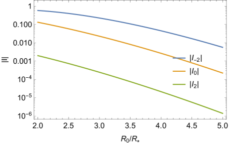
Figure 1: $|I_{\pm 2}|$ and $|I_{0}|$ (Eq. (29)) as functions of $R_{0}/R_{*}$. In the Newtonian limit, when $R_{0}=2R_{*}$ the surfaces of two undeformed stars are in marginal contact at the periastron passage.

With the excitation coefficients shown in Fig. 1, and the overlap constants obtained from Eq. (49), we can write the mode energy in Eq. (II.2.1) as

$$\Delta E_{\rm mode} =0.587\frac{GM^{2}R^{2}_{*}}{R^{3}_{0}}[I^{2}_{-2}(\varpi_{22})+I^{2}_{2}(\varpi_{22})]\,$$

$$+0.391\frac{GM^{2}R_{*}^{2}}{R^{3}_{0}}I^{2}_{0}(\varpi_{20})\,.$$ (51)

and mode angular momentum

$$\Delta J_{\rm mode} =0.478\frac{G^{1/2}M^{3/2}R^{7/2}_{*}}{R^{3}_{0}}[I^{2}_{-2}(\varpi_{22})-I^{2}_{2}(\varpi_{22})]\,.$$ (52)

Without considering mode excitations, the GW energy emitted during a periastron passage can be estimated as Peters (1964); Chirenti et al. (2017):

$$\Delta E_{\rm GW}\approx 7\pi\frac{(GM)^{7/2}M}{c^{5}R_{0}^{7/2}}\,,$$ (53)

and the angular momentum carried away by GWs is

$$\Delta J_{\rm GW}\approx 6\pi\frac{(GM)^{3}M}{c^{5}R_{0}^{2}}\,.$$ (54)

As a result, the ratio between the mode energy deposited into both stars and the energy carried away by GWs during the main burst is

$$\frac{2\Delta E_{\rm mode}}{\Delta E_{\rm GW}}\approx \left(\frac{GM}{c^{2}R_{*}}\right)^{-5/2}\left(\frac{R_{0}}{R_{*}}\right)^{1/2}\times 2\times 10^{-2}\times$$

$$\left\{2.69[I^{2}_{-2}(\varpi_{22})+I^{2}_{2}(\varpi_{22})]+1.78I^{2}_{0}(\varpi_{20})\right\}\,.$$ (55)

Similarly, the ratio between the mode angular momentum deposited into both stars and the angular momentum carried away by GWs during the main burst is

$$\frac{2\Delta J_{\rm mode}}{\Delta J_{\rm GW}}\approx \left(\frac{GM}{c^{2}R_{*}}\right)^{-5/2}\left(\frac{R_{0}}{R_{*}}\right)^{-1}\times 0.05\times$$

$$\left\{[I^{2}_{-2}(\varpi_{22})-I^{2}_{2}(\varpi_{22})])\right\}\,.$$ (56)

The dominant contribution comes from the $m=-2$ mode with our conventions. As a concrete example, take a NS with compaction $GM/(c^{2}R_{*})\sim 0.17$ (e.g. $M\approx 1.4$ $M_{\odot}$ and $R_{*}\approx 12$ km). In Fig. 2 we plot the ratio described in Eq. (III.1) and Eq. (III.1) as a function of the “periastron frequency” $f$ (of the orbit, hence half the GW frequency). This frequency is introduced in Loutrel and Yunes (2017); Chirenti et al. (2017) (also discussed in Sec. IV), and represents the peak frequency of the main burst. In the Newtonian limit, $f$ is proportional to $R_{0}^{-1.5}$. In Fig. 2, $f_{c}:=\sqrt{M/(2R_{*})^{3}}/\pi$ denotes the periastron frequency for the closest possible passage without the stars colliding. For comparison, in this figure we also show results from the full numerical solutions described in Sec. IV. These agree with the model to within a factor of two, even at the relativistic velocities considered. The plot shows that, for very close pericenter passages, the mode energy/angular momentum deposited into the stars can be of the same order of magnitude as the energy/angular momentum carried away by GWs. This means that it is crucial to include the mode dynamics in order to accurately model the orbital evolution.

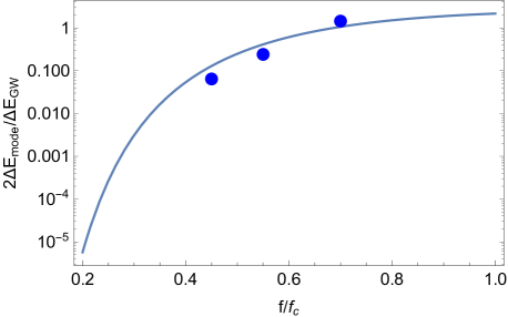
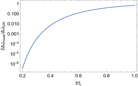
Figure 2: The ratio between the total mode energy (angular momentum) deposited onto stars and the energy (angular momentum) carried away by GWs during the main burst, as a function of the normalized periastron frequency $f/f_{c}$. Here $R_{*}c^{2}/(GM)$ is taken to be $5.88$. The dots shown in the top plot represent estimates from the numerical simulations listed in Table. 1.

IV Simulations in full GR

In order to validate the model described in the previous section, and determine its accuracy into the relativistic regime, we simulate several cases consisting of compact object binaries undergoing a close encounter using GR coupled to hydrodynamics. This work makes use of similar methods to those of previous studies of eccentric binary mergers East et al. (2012a); East and Pretorius (2012); Paschalidis et al. (2015); East et al. (2016a, b), which we just briefly review here.

IV.1 Numerical Methods

These simulations are carried out by solving the full Einstein equations coupled to hydrodynamics using the methods described in East et al. (2012b). For ease of comparison to the approximate model described in this work, we restrict ourselves to a $\Gamma=2$ EOS. We make use of adaptive mesh refinement with seven levels of refinement. The base-level resolution has $201^{3}$ points, while the finest-level resolution has approximately $100$ points across the NS diameter. For simulations with BHs, we use one additional mesh refinement level, which gives a factor of two better resolution, around the BH. For one of the NS-NS cases, we also perform a lower resolution simulation with $0.6\times$ the above resolution, in order to estimate truncation error.

IV.2 Initial Data and Cases

We study binary NS close encounters with several different impact parameters, and then follow the oscillations in the stars during the long outgoing part of the elliptic orbit. For comparison, we also consider an equal mass BH-NS case with a non-spinning BH and the same orbital parameters as one of the binary NS cases. Initial data is constructed using the methods described in East et al. (2012c). We choose the initial velocities and positions of the compact objects at large separation ($d=50M_{\rm tot}$, where $M_{\rm tot}$ is the total mass of the system) based on a marginally bound Newtonian orbit with a specified periapse distance $R_{0}$. The actual periapse distance of the binary will be different (due to gauge effects, relativistic corrections, etc.), and we fix the parameters used for comparing to the approximate model based on the frequency of the fly-by gravitational waveform. This allows a largely gauge-invariant comparison with the model we presented in the previous section. We consider several equal mass binary NS cases with $R_{0}/M_{\rm tot}=10.0$, 11.5, and 13. For the comparison to an equal mass BH-NS system, we use a single NS case with $R_{0}/M_{\rm tot}=11.5$. In all cases we choose a NS with $M_{*}/R_{*}=0.17$.

IV.3 Results

In Fig. 3 we show a comparison of the GWs from a NS-NS and BH-NS case with the same orbital parameters. The fly-by part of the waveform matches well between the two cases, indicating that the incoming orbits are very close. The peak instantaneous GW frequency, calculated from the time derivative of the phase of the $(2,2)$ component of $\Psi_{4}$ is $\omega M_{\rm tot}=0.11$, and differs by $<1\%$ in the two cases. This corresponds to normalized periastron frequency of $f/f_{c}=0.55$. The amount of energy radiated in GWs around the periapse passage is $\Delta E_{\rm GW}/M_{\rm tot}\approx 6.4\times 10^{-4}$.

After the fly-by there are high frequency GW oscillations in both cases. By going to the frequency domain we can see these GW oscillations are primarily at the expected $f$-mode frequency, and that the amplitude in the binary NS case is twice that of the BH-NS case, indicating that to a good approximation the stars are tidally perturbed by the same amount. In the middle panel of Fig. 3, one can see a lower frequency modulation in the GW signal. The fact that this occurs in both the binary NS and BH-NS cases indicates that it is not due to interference effects, and is perhaps instead due to the presence of more than one fluid oscillation mode.

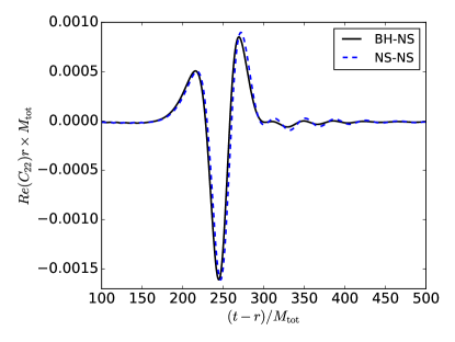
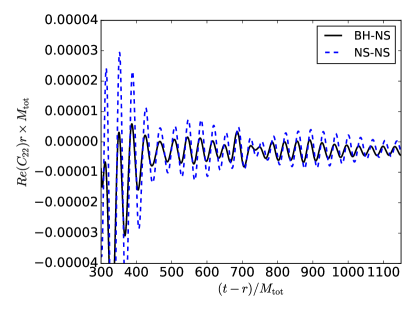
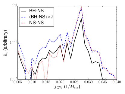
Figure 3: A comparison of the GWs from a BH-NS and NS-NS case with $R_{0}/M_{\rm tot}=11.5$. The top and middle panels show the real part of the $(2,2)$ component of $\Psi_{4}$, the former emphasizing the GW burst from the close encounter, and the latter emphasizing the GW oscillations from the $f$-mode excitations in the NS(s). The bottom panel shows the post fly-by GWs ($t-r>500M_{\rm tot}$) in the frequency domain. The peak at approximately $f_{\rm GW}\approx 0.027/M_{\rm tot}$ associated with the $f$-mode oscillations is a factor of two larger in the binary NS case, as expected if the NSs are tidally perturbed by the same amount in both cases.

We can estimate the amount of energy lost to tidal excitations by comparing the orbits in the two cases. In Fig. 4 we show the coordinate separation of the binary as a function of angle, at large values post-flyby. Fitting this to a Newtonian orbit, and taking the difference of the resulting values for the orbital energy for the BH-NS and NS-NS cases and attributing it to the energy of the tidal excitations in a single star gives $\Delta E_{\rm mode}/\Delta E_{\rm GW}=0.13$. In comparison, the analytic model predicts $\Delta E_{\rm mode}/\Delta E_{\rm GW}=0.22$.

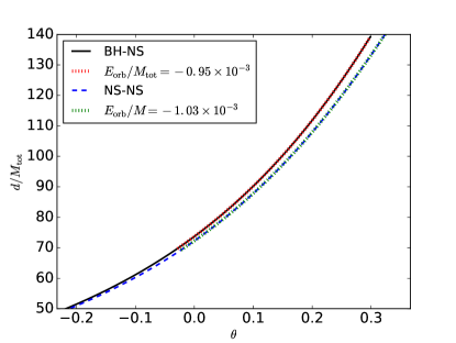
Figure 4: The coordinate separation versus orbital angle at large distances post-flyby for a BH-NS and NS-NS system with the same initial binary parameters. We also show the Newtonian orbits with the best-fit parameters for these two cases.

We use the above estimate of $\Delta E_{\rm mode}$ as a reference value, and also consider how the tidal excitation compares as a function of impact parameter —or equivalently, periastron frequency—for a higher and lower case. The results are summarized in Table 1. All cases show the expected peak in the characteristic strain at the f-mode frequency as in the bottom panel of Fig. 3, and here we have estimated $\Delta E_{\rm mode}$ by assuming that it is proportional to the strain within this peak (within $10\%$ of the f-mode frequency), and using the above comparison to the BH-NS to fix the overall magnitude. We also note that by comparing two different resolutions for the largest impact parameter (lowest value of $f/f_{c}$ case), and assuming second order convergence , we estimate that the truncation error in the calculation of $\Delta E_{\rm mode}$ is $\sim 20\%$ (and it is an underestimated), while the truncation errors in $f/f_{c}$ and $E_{\rm GW}$ are smaller, $\lesssim 1\%$. Likely more significant are systematic effects in estimating orbital energy based on comparing coordinate trajectories for the BH-NS and NS-NS cases, and measuring tidal excitations based on the GW emission. Since our main purpose here is to establish the rough accuracy of the analytic model for tidal excitations, we leave a more in-depth study of this to future work.

Table 1: The first two columns are the characteristic frequency and energy emitted in GWs during pericenter passage. The last two columns are an estimate of the amount of energy deposited in tidal excitations (per star) from three equal-mass, nearly parabolic binary NS encounters from the full GR calculation and the analytic model.

$f/f_{c}$	$\Delta E_{\rm GW}/M_{\rm tot}$	$\Delta E_{\rm mode}/\Delta E_{\rm GW}$ (sims.)	(model)
0.70	$15.0\times 10^{-4}$	0.72	0.53
0.55	$6.4\times 10^{-4}$	0.12	0.22
0.45	$3.4\times 10^{-4}$	0.032	0.06

V Trajectory model

A trajectory and waveform model for highly eccentric, binary BH systems was developed in Loutrel and Yunes (2017). The key idea is to divide the whole trajectory into a series of PN elliptical orbits attached by a change of orbital parameters that occurs during the pericenter passage process. The shift of orbital eccentricity and energy/angular momentum can be obtained by computing the accumulated GW flux within each cycle.

Based on a PN description of the orbital evolution, the BH waveform model then contains four physical quantities: $t_{i},\delta t_{i},f_{i},\delta f_{i}$ for the $i$th cycle. Here $t_{i}$ is the coordinate time for the $i$th periastron passage while $f_{i}$ is the “periastron frequency”, defined as Loutrel and Yunes (2017)

$$f_{i}\equiv\frac{1}{2\pi\tau_{\rm GW}}\equiv\frac{1}{2\pi}\frac{\rm pericenter\,\,\,velocity}{\rm pericenter\,\,\,distance}\,,$$ (57)

which reduces to

$$f_{i}=\frac{1}{2\pi}\frac{[(M+M_{*})(1+e)]^{1/2}}{R_{0}^{3/2}}$$ (58)

in the Newtonian limit.

Phenomenologically, $2f_{i}$ well approximates the central burst frequency of GWs corresponding to the $i$th periastron passage. With the predictions of $t_{i}$ and $f_{i}$ for the central arriving time and frequency of each GW burst, one can extract a sequence of centroids of size $\delta t_{i}\times\delta f_{i}$ in the time-frequency diagram around $(t_{i},f_{i})$, compute the spectrum within each centroid, and possibly stack the spectra power of different centroids to boost the total signal-to-noise ratio East et al. (2013); Huerta et al. (2014). The choices for $\delta t_{i}$ and $\delta f_{i}$ are rather flexible; in Loutrel and Yunes (2017) they are chosen to be constant multiples of $\tau_{\rm GW}$ and $f_{i}$.

We notice that if the orbital evolution and GW emission can be modeled with enough accuracy, such that the phase error of the waveform for the whole duration is controlled within $\mathcal{O}(1/{\rm SNR})$ (with ${\rm SNR}$ being the signal-to-noise ratio of a typical event), it is preferable to use a single waveform covering the whole duration for both detection and parameter estimation purpose. This requirement is challenging because the binary dynamics could be quite nonlinear near pericenter passages, and the total duration could contain many cycles. It is computationally prohibitive to perform numerical simulations of this type to calibrate the theoretical waveforms designed for such systems. Nevertheless, one possibility is to use a waveform calibrated by numerical relativity when the NSs are close to each other, and then match it to a PN waveform when the two stars are far apart. We shall leave further investigation of this to future work.

V.1 Order of magnitude estimates

As discussed in Sec. III, and explicitly shown in Fig. 2, the energy/angular momentum deposited into the stars may be of the same order of magnitude as the energy/angular momentum carried away by GWs during close pericenter passages. In this case it is necessary to include the effect of mode excitations into the evolution model for such orbits.

To quantify the regime of importance for mode excitations, we notice that $2\Delta E_{\rm mode}/\Delta E_{GW}$ in Fig. 2 exceeds $1\%$ only when $f/f_{c}\geq 1/3$, which means that

$$f\geq\frac{f_{c}}{3}\sim 3.9\times 10^{2}{\rm\ Hz}\left(\frac{M}{1.4\ M_{\odot}}\right)^{1/2}\left(\frac{R_{*}}{12{\rm\ km}}\right)^{-3/2}\,.$$ (59)

Another question is whether it is necessary to include the oscillations inherited from the previous pericenter passage as in Eq. (II.2.2) and Eq. (II.2.2), instead of setting $A_{\rm init}$ and $\dot{A}_{\rm init}$ to be zero before each pericenter passage. To answer this question, we compare the mode decaying timescale $1/\gamma_{22}$ with the orbital period (in the Newtonian limit)

$$T =2\pi\left[\frac{G(M+M_{*})}{a_{0}^{3}}\right]^{-1/2}$$

$$=2\pi\left[\frac{G(M+M_{*})}{R_{0}^{3}}\right]^{-1/2}(1-e)^{-3/2}\,.$$ (60)

We conclude that the initial oscillations are negligible if (assuming $M=M_{*}$)

$$1-e\ll 0.63\frac{R_{0}}{R_{*}}\left(\frac{GM}{R_{*}c^{2}}\right)^{5/3}\,.$$ (61)

If we consider the type of NS assumed to produce Fig. 2 and consider the closest passage with $R_{0}=2R_{*}$, the above inequality can be translated to $1-e\ll 0.07$. For such binaries (with Eq. (61) satisfied), it is no longer necessary to track the evolution of modes, as the lifetime of the modes is smaller than the time between pericenter passages. However, in order to compute the energy and angular momentum change of the orbit after pericenter passages, it is still necessary to include the mode contributions using Eq. (II.2.2) and Eq. (II.2.2), with $A_{\rm init}$ and $\dot{A}_{\rm init}$ set to zero.

In the special case studied in Sec. IV, the two NSs are assumed to be identical, which means that their f-modes have the same frequency. The GWs generated by f-mode oscillations from two stars may beat with each other, depending on the separation of two stars and the sky direction of observers. This beating starts to become important if the orbital separation is comparable to, or larger than, the half-wavelength of the f-mode GWs:

$$1\leq\frac{a_{0}(1+e)}{\lambda/2}\approx\frac{2R_{0}\omega_{22}}{\pi(1-e)c}\,,$$ (62)

or equivalently

$$1-e\leq 0.78\frac{R_{0}}{R_{*}}\left(\frac{GM}{R_{*}c^{2}}\right)^{1/2}\,.$$ (63)

In reality, the masses of individual NSs within the binary will be different (we denote the mass difference as $\Delta M=M-M_{*}$). According to the f-mode frequency formula (see Eq. (48)), we have $\delta f/f\sim 0.5\Delta M/M$. The beating generally loses constructive interference after $f/2\delta f\sim M/\Delta M$ oscillation cycles.

V.2 Trajectory model

The quasi-Keplerian (QK) description of eccentric orbits of a compact binary is well explained in Blanchet (2014). In this framework, the 1PN motion of the binary in the radial, time, and angular directions can be written in the following form:

$$r =a_{r}(1-e_{r}\cos u)\,$$

$$\ell =u-e_{t}\sin u+\mathcal{O}(c^{-4})\,,$$

$$\frac{\phi-\phi_{p}}{K} =v+\mathcal{O}(c^{-4})=2\arctan\left[\left(\frac{1+e_{\phi}}{1-e_{\phi}}\right)^{1/2}\tan\frac{u}{2}\right]\,,$$ (64)

where $v$ is the true anomaly, $u$ is the eccentric anomaly, $\ell=n(t-t_{p})$ is the mean anomaly with $n=2\pi/T$ being the mean motion, and $P$ is the period. In addition, $K$ is related to the periastron precession angle per cycle $\Delta\phi_{p}$ by $\Delta\phi_{p}=2\pi(K-1)$. The above QK representation has been generalized to 2 PN Damour and Schäeer (1988); Schäfer and Wex (1993); Wex (1995) and 3 PN orders Memmesheimer et al. (2004). The orbital eccentricities $e_{t}$, $e_{r}$, and $e_{\phi}$, and additional parameters $n$, $K$, and $a_{r}$ are all functions of the orbital energy and angular momentum (see Eq. (345) in Blanchet (2014)), and we introduce a new set of parameters to match the convention in Blanchet (2014):

$$\epsilon=-\frac{2E}{\mu c^{2}},\quad j=-\frac{2Eh^{2}}{\mu^{3}},$$ (65)

with $\mu=(M+M_{*})\nu$, $\nu=MM_{*}/(M+M_{*})^{2}$ and $h=J/G(M+M_{*})$. In order to obtain a mapping for orbital parameters from one cycle to the next, we first compute the energy and angular momentum change within the current cycle:

$$E_{i+1} =E_{i}+\Delta E_{\rm GW,i}+\Delta E_{\rm mode,i}\,$$

$$J_{i+1} =J_{i}+\Delta J_{\rm GW,i}+\Delta J_{\rm mode,i}\,.$$ (66)

The energy and angular momentum radiated by the orbital motion within the $i$th cycle are

$$\Delta E_{\rm GW,i} =\langle\dot{E}_{\rm GW,i}\rangle T_{i}=\langle\dot{E}_{\rm GW,i}\rangle\frac{2\pi}{n_{i}}\,,$$

$$\Delta J_{\rm GW,i} =\langle\dot{J}_{\rm GW,i}\rangle\frac{2\pi}{n_{i}}$$ (67)

where $n_{i}$ is given by Eq. ($347a$) in Blanchet (2014). The 3PN orbital-averaged energy flux can be obtained from Eq. ($355$) in Blanchet (2014), and the 3PN averaged angular momentum can be found in Arun et al. (2009). For the mode energy and angular momentum change we use Eq. (II.2.2), Eq. (II.2.2) and Eq. (65). There is however one subtlety, which is to include the residual oscillation from the previous pericenter passage into the calculation, i.e., the terms involving $A_{\rm init}$ and $\dot{A}_{\rm init}$. Based on Eq. (II.2.1), we denote $A_{\rm init,i}=A_{\rm init}(t_{i}),\,\dot{A}_{\rm init,i}=\dot{A}_{\rm init}(t_{i})$, and explicitly write down their mapping relations as (with $Q\gg 1$)

$$A^{22}_{\rm init,i+1} =\left[A^{22}_{\rm init,i}+i\sqrt{3\pi/10}\frac{M_{*}}{na^{3}_{r}}Q_{\xi}(P_{-2}-P_{2})\right]\left[\cos(\omega T_{i})+\frac{\gamma}{\omega}\sin(\omega T_{i})\right]e^{-\gamma T_{i}}$$

$$+\left[\sqrt{3\pi/10}\frac{M_{*}}{na^{3}_{r}}Q_{\xi}(P_{-2}+P_{2})+\dot{A}^{22}_{\rm init,i}\right]\frac{\sin(\omega T_{i})}{\omega}e^{-\gamma T_{i}}$$

$$\dot{A}^{22}_{\rm init,i+1} =\left[\sqrt{3\pi/10}\frac{M_{*}}{na^{3}_{r}}Q_{\xi}(P_{-2}+P_{2})+\dot{A}^{22}_{\rm init,i}\right]\left[\cos(\omega T_{i})-\frac{\gamma}{\omega}\sin(\omega T_{i})\right]e^{-\gamma T_{i}}$$

$$-\left[A^{22}_{\rm init,i}+i\sqrt{3\pi/10}\frac{M_{*}}{na^{3}_{r}\omega}Q_{\xi}(P_{-2}-P_{2})\right]\omega\sin(\omega T_{i})e^{-\gamma T_{i}}\,,$$ (68)

with $A^{22}_{\rm init,i}=A^{2,-2*}_{\rm init,i},\dot{A}^{22}_{\rm init,i}=\dot{A}^{2,-2*}_{\rm init,i}$ and similarly

$$A^{20}_{\rm init,i+1} =A^{20}_{\rm init,i}\left[\cos(\omega T_{i})+\frac{\gamma}{\omega}\sin(\omega T_{i})\right]e^{-\gamma T_{i}}$$

$$+\left[-\sqrt{4\pi/5}\frac{M_{*}}{na^{3}_{r}}Q_{\xi}P_{0}+\dot{A}^{20}_{\rm init,i}\right]\frac{\sin(\omega T_{i})}{\omega}e^{-\gamma T_{i}}\,,$$

$$\dot{A}^{20}_{\rm init,i+1} =\left[-\sqrt{4\pi/5}\frac{M_{*}}{na^{3}_{r}}Q_{\xi}P_{0}+\dot{A}^{20}_{\rm init,i}\right]\left[\cos(\omega T_{i})-\frac{\gamma}{\omega}\sin(\omega T_{i})\right]e^{-\gamma T_{i}}$$

$$-A^{20}_{\rm init,i}\omega\sin(\omega T_{i})e^{-\gamma T_{i}}\,,$$ (69)

where we have abbreviated the mode index for frequencies and decay rates because they are the same for all modes with $\ell=2$.

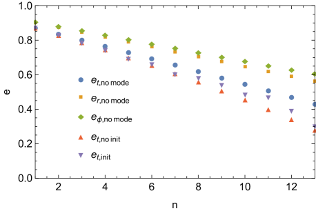
Figure 5: Plot of PN eccentricities for a sequence of pericenter passages, indexed by $n$. The quantities $e_{t}$, $e_{r}$, and $e_{\phi}$ are not gauge-invariant and their values are given in modified harmonic coordinates. The initial pericenter separation is $R_{0,1}=3R_{*}$, and the initial $e_{r}$ is set to $0.9$. The quantities $e_{\rm t,no\,mode}$, $e_{\rm r,no\,mode}$, and $e_{\rm\phi,no\,mode}$ are obtained without including the star’s oscillations; $e_{\rm t,no\,init}$ is computed including the star’s oscillation but zero $A_{\rm init}$; $e_{\rm t,init}$ is computed taking into account the evolution of the mode amplitude over time.

In reality, even if the initial mode oscillation is known at the beginning of a sequence of bursts, the phase error due to the PN approximation and the osculating orbit approximation may accumulate with time and eventually lead to very inaccurate predictions for $A_{\rm init}$ and $\dot{A}_{\rm init}$. As a result, if we denote the time for a template to receive $\mathcal{O}(1)$ phase error as $\tau_{1}$, an accurate template should satisfy $\tau_{1}\gamma_{22}>1$.

To 1PN order, the periastron frequency of the $i$th cycle $f_{i}$ is given by Loutrel and Yunes (2017)

$$f_{i} \equiv\frac{1}{2\pi}\frac{\rm pericenter\,\,\,velocity}{\rm pericenter\,\,\,distance}\,$$

$$=\frac{1}{2\pi}\sqrt{\frac{1+e_{\phi}}{1-e_{\phi}}}\frac{nK}{1-e_{t}}\,.$$ (70)

At 3 PN order, $f_{i}$ can be obtained by combining Eq.  ($346$) and Eq. ($343$) in Blanchet (2014):

$$f_{i} =\frac{n}{2\pi}\frac{d\phi/du}{d\ell/du}=\frac{nK}{2\pi}\left.\frac{dv}{du}\right|_{u=0}\left.\frac{1+2f_{\phi}\cos 2v+3g_{\phi}\cos 3v+4i_{\phi}\cos 4v+5h_{\phi}\cos 5v}{1-e_{t}\cos u-g_{t}+dv/du(g_{t}+f_{t}\cos v+2i_{t}\cos 2v+3h_{t}\cos 3v)}\right|_{u,v=0}$$

$$=\frac{nK}{2\pi}\sqrt{\frac{1+e_{\phi}}{1-e_{\phi}}}\frac{1+2f_{\phi}+3g_{\phi}+4i_{\phi}+5h_{\phi}}{1-e_{t}-g_{t}+\sqrt{\frac{1+e_{\phi}}{1-e_{\phi}}}(g_{t}+f_{t}+2i_{t}+3h_{t})}\,,$$ (71)

where the definition and more discussions on the orbital elements $f_{\phi},g_{\phi},i_{\phi},h_{\phi},f_{t},g_{t},i_{t},h_{t},e_{t},e_{r},e_{\phi}$ can be found in Blanchet (2014); Memmesheimer et al. (2004).

Under the impulsive approximation, the Newtonian formula for the energy and angular momentum deposited into the stars, i.e., Eq. (II.2.2) and Eq. (II.2.2), can be further improved by incorporating the 1PN trajectory description in Eq. (V.2). To do that, we only need to replace $a_{0}$ in Eq. (II.2.2), (II.2.2) by $a_{r}$, and the definition of $P_{m}(y)$ to be

$$P_{m}(y)=\int^{\pi}_{0}\,\frac{dx}{(1-e_{r}\cos x)^{2}}\times\cos{\left\{y\frac{x-e_{t}\sin x}{n}+2mK\arctan\left[\left(\frac{1+e_{\phi}}{1-e_{\phi}}\right)^{1/2}\tan\frac{u}{2}\right]\right\}}\,,$$ (72)

and $\Delta E_{\rm mode}$ and $\Delta J_{\rm mode}$ are explicitly given by

$$\Delta J_{\rm mode,z} =|Q^{22}_{\xi}|^{2}\frac{3\pi}{5\omega_{22}}\frac{M^{2}_{*}}{n^{2}a^{6}_{r}}[P^{2}_{-2}(\omega_{22})-P^{2}_{2}(\omega_{22})]+\frac{2\sqrt{6\pi/5}M_{*}}{a^{3}_{r}n}[P_{-2}(\omega_{22})+P_{2}(\omega_{22})]{\rm Im}[A^{(22)}_{\rm init}Q^{22}_{\xi}]$$

$$+\frac{2\sqrt{6\pi/5}M_{*}}{\omega_{22}a^{3}_{r}n}[P_{-2}(\omega_{22})-P_{2}(\omega_{22})]{\rm Re}[\dot{A}^{(22)}_{\rm init}Q^{22}_{\xi}]\,,$$ (73)

and

$$\Delta E_{\rm mode} =|Q^{22}_{\xi}|^{2}\frac{3\pi}{5}\frac{M^{2}_{*}}{n^{2}a^{6}_{r}}[P^{2}_{-2}(\omega_{22})+P^{2}_{2}(\omega_{22})]+|Q^{20}_{\xi}|^{2}\frac{2\pi}{5}\frac{M^{2}_{*}}{n^{2}a^{6}_{r}}P^{2}_{0}(\omega_{20})\,$$

$$+\frac{\omega_{22}\sqrt{6\pi/5}M_{*}}{a^{3}_{r}n}[P_{-2}(\omega_{22})-P_{2}(\omega_{22})]{\rm Im}[A^{(22)}_{\rm init}Q^{22}_{\xi}]+\frac{\sqrt{6\pi/5}M_{*}}{a^{3}_{r}n}[P_{-2}(\omega_{22})+P_{2}(\omega_{22})]{\rm Re}[\dot{A}^{(22)}_{\rm init}Q^{22}_{\xi}]$$

$$-\frac{2\sqrt{\pi/5}M_{*}}{a^{3}_{r}n}\dot{A}^{(20)}_{\rm init}Q^{20}_{\xi}P_{0}(\omega_{20})\,.$$ (74)

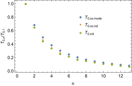
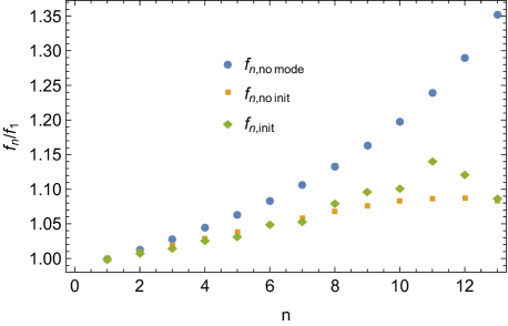
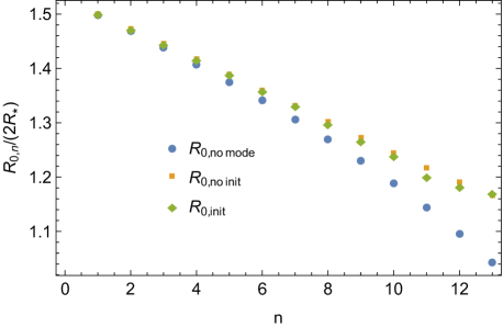
Figure 6: The same set-up as Fig. 5. The top plot represents the evolution of the orbital period; the middle panel represents the evolution of the pericenter frequency; the bottom panel represents the evolution of the pericenter distance.

Note that in order to capture higher PN tidal effects, the analysis on stellar oscillation in Appendix A should be extended to higher PN orders as well. In order to illustrate the trajectory model described by Eqs. (II.2.2), (II.2.2), (V.2), (V.2), (V.2), (V.2), we start an orbit with initial pericenter distance $R_{0}=3R_{*}$ and initial eccentricity $e_{r}=0.9$ (in the modified harmonic coordinate; this quantity is not gauge-invariant). In Fig. 5, we compare the evolution of eccentricities in three different scenarios: (i) assuming no tidal excitations of the stars, (ii) allowing stellar oscillations, while neglecting the non-zero values of $A_{\rm init}$ and $\dot{A}_{\rm init}$ from previous encounters, (iii) allowing star oscillations and evolving $A_{\rm init}$ and $\dot{A}_{\rm init}$. In Fig. (6), we also present the evolution of the orbital period, pericenter frequency, and pericenter distance for the above three scenarios. We can see that for such a close encounter, the oscillation of the stars significantly alters the trajectory, and it is important to include the evolution of the modes into the trajectory model. In fact, for this case during some of the later close encounters, the frequency of the orbit is larger when this evolution is tracked, compared to when it is not, as energy and angular momentum are taken out of the NS oscillations and put back in the orbit. We also notice that, for the last several orbits, the eccentricity falls below $0.5$. Strictly speaking, orbits in such a regime are no longer highly eccentric, since the impulsive approximation is no longer accurate. To deal with orbits with mid-range eccentricities, the mode evolution has to be computed using a continuous forcing in time. Studying this regime is beyond the scope of this paper.

VI Conclusion

In this work, we have shown that tidal excitation of stellar modes can dramatically influence the dynamics of binary neutron stars in highly eccentric orbits. The amount of extra energy and angular momentum change in the orbit due to mode excitation can be tens of percent of that due to GWs alone, if the pericenter distance is smaller than $\sim 4R_{*}$. The exact amounts will depend on the EOS, and here we focused on a $\Gamma=2$ polytrope to simplify the comparison between the analytic model and numerical results. The prediction from the Newtonian approximation agrees with the full numerical results to within a factor of a two (with the error likely dominated by systematic effects in measuring orbital properties from the code results). This also resolves the large discrepancy between a similar analytic calculation and numerical simulations reported in Chirenti et al. (2017).

The discussion presented in this work also applies for highly eccentric NS-BH binaries, regardless of the mass ratio Yang et al. (2018b). While the rates of detecting these highly eccentric binaries are uncertain, their gravitational waveforms display distinctive f-mode oscillations, which are not present in any appreciable amount in quasi-circular systems. Observing these oscillations would provide unprecedented information about the structure and EOS of cold NSs. One possible way to enhance the SNR of these oscillation features is to stack the post-encounter waveform of a series of pericenter passages, which requires accurate predictions for the timing of these encounters. Another possibility is to rely on the observation of third-generation ground-based detectors. As the f-mode frequency is generally above 2 kHz (the f-mode frequency in Fig. 3 is approximately 2.6 kHz), the high frequency detector proposed in Miao et al. (2017) is ideal for observing such signals. Assuming a detection strategy that coherently adds the signals from different pericenter encounters, the estimated SNR for f-mode oscillations is

$${\rm SNR}\sim \,30\left(\frac{\mathcal{E}_{mode}}{\mathcal{E}_{\rm GW}}\right)^{1/2}\left(\frac{50{\rm\ Mpc}}{d}\right)\left(\frac{5\times 10^{-25}{\rm\ Hz}^{-1/2}}{\sqrt{S_{n}}}\right)$$

$$\times\left(\frac{2000{\rm\ Hz}}{f}\right)\,,$$ (75)

where $d$ is the distance of the binary from Earth, $S_{n}$ is the one-sided power spectral density of the detector, $\mathcal{E}_{\rm GW}$ is the total energy radiated by GWs and $\mathcal{E}_{mode}$ is the energy radiated by f-mode oscillations.

Appendix A Perturbations of a polytropic star

The perturbation of a polytropic star is described by the Lagrangian displacement field ${\bf\xi}$, which obeys (Eq. (2.212) of Poisson and Will (2014)):

$$\partial^{2}_{t}\xi=\left(\frac{\delta\rho}{\rho^{2}}\right)\nabla\rho-\frac{\nabla\delta p}{\rho}-\nabla\delta\Phi\,,$$ (76)

where

$$\delta p =-\Gamma_{p}p\nabla\cdot\xi-\xi\cdot\nabla p\,$$

$$\delta\rho =-\nabla\cdot(\rho\xi)\,.$$ (77)

Here $\Gamma_{p}$ is the adiabatic index of the perturbation, which may or may not be the same as $\Gamma$ for the equilibrium configuration. However, for the polytropic (hence barotropic) stars studied here, we have $\Gamma=\Gamma_{p}$. In addition, the total Newtonian potential is $\delta\Phi=\delta U+U_{\rm tide}$, where $\delta U$ obeys the Poisson equation:

$$\nabla^{2}\delta U=-4\pi G\delta\rho\,.$$ (78)

The equation of motion for the Lagrangian displacement field can be written schematically as

$$\partial^{2}_{t}\xi_{j}+{L_{j}}^{k}\xi_{k}=\nabla_{j}U_{\rm tide}\,.$$ (79)

In order to determine the body’s response to an applied tidal field, it is useful to first compute the normal modes of the system, corresponding to free oscillations, i.e. solutions of Eq. (79) with the right-hand side being zero. With $\xi^{(n)}$ given in Eq. (5), we write $\xi_{j}$ as $\xi^{(n)}_{j}e^{i\sigma t}$, and define

$$\delta p =\rho(r)\,y(r)Y_{lm}(\theta,\phi)e^{i\sigma t}\,,$$

$$\delta\rho =\varrho(r)Y_{lm}(\theta,\phi)e^{i\sigma t}\,,$$

$$\delta U =u(r)Y_{lm}(\theta,\phi)e^{i\sigma t}\,.$$ (80)

When combining Eqs. (76) and (78), we notice that not all perturbation variables are independent. In particular, we can express $\xi_{S}$ and $\varrho$ in terms of the other variables as

$$\xi_{S}=\frac{y+u}{r\sigma^{2}}\,,\quad\varrho=\frac{\rho^{2}y}{\Gamma_{p}p}-A\xi_{R}\,.$$ (81)

We obtain the following ordinary differential equations:

$$(r^{2}\xi_{R})^{\prime} =-\frac{r^{2}p^{\prime}\xi_{R}}{\Gamma_{p}p}+\left[\frac{l(l+1)}{\sigma^{2}}-\rho\frac{r^{2}}{\Gamma_{p}p}\right]y+\frac{l(l+1)u}{\sigma^{2}}\,,$$

$$y^{\prime} =(\sigma^{2}+Ag)\xi_{R}-Ay-u^{\prime}\,,$$

$$u^{\prime\prime} =-\frac{2}{r}u^{\prime}+\frac{l(l+1)u}{r^{2}}+4\pi G\rho\left(\frac{\rho y}{\Gamma_{p}p}-A\,\xi_{R}\right)\,$$ (82)

with

$$g\equiv-\frac{p^{\prime}}{p},\quad A\equiv\frac{\rho^{\prime}}{\rho}-\frac{p^{\prime}}{\Gamma_{p}p}\,.$$ (83)

As explained above, for the polytropic stars studied here, $A$ is zero. The differential equations are subject to the regularity condition at the center of star and boundary conditions at the stellar surface which require force balance and zero pressure:

$$(\rho\,y+p^{\prime}\xi_{R})|_{R_{*}}=0,$$

$$\left.\left(u^{\prime}+(l+1)\frac{u}{r}\right)\right|_{R_{*}}=-4\pi G\rho(R_{*})\xi_{R}(R_{*})\,.$$ (84)

The eigenfrequency $\sigma$ and eigenfunctions $\xi_{R}$ and $\xi_{S}$ can be obtained by solving Eqs. (A) with the above boundary conditions.

References

- Abbott et al. (2016a) B. P. Abbott et al. (Virgo, LIGO Scientific), Phys. Rev. Lett. 116, 061102 (2016a), eprint 1602.03837.
- Abbott et al. (2016b) B. P. Abbott et al. (Virgo, LIGO Scientific), Phys. Rev. Lett. 116, 241103 (2016b), eprint 1606.04855.
- Abbott et al. (2017a) B. P. Abbott, R. Abbott, T. D. Abbott, F. Acernese, K. Ackley, C. Adams, T. Adams, P. Addesso, R. X. Adhikari, V. B. Adya, et al. (LIGO Scientific and Virgo Collaboration), Phys. Rev. Lett. 118, 221101 (2017a), URL https://link.aps.org/doi/10.1103/PhysRevLett.118.221101.
- Abbott et al. (2017b) B. Abbott, R. Abbott, T. Abbott, F. Acernese, K. Ackley, C. Adams, T. Adams, P. Addesso, R. Adhikari, V. Adya, et al., The Astrophysical Journal Letters 851, L35 (2017b).
- Abbott et al. (2017c) B. P. Abbott, R. Abbott, T. Abbott, F. Acernese, K. Ackley, C. Adams, T. Adams, P. Addesso, R. Adhikari, V. Adya, et al., Physical review letters 119, 141101 (2017c).
- Abbott et al. (2017d) B. P. Abbott, R. Abbott, T. Abbott, F. Acernese, K. Ackley, C. Adams, T. Adams, P. Addesso, R. Adhikari, V. Adya, et al., Physical Review Letters 119, 161101 (2017d).
- O’Leary et al. (2009) R. M. O’Leary, B. Kocsis, and A. Loeb, Monthly Notices of the Royal Astronomical Society 395, 2127 (2009).
- Lee et al. (2010) W. H. Lee, E. Ramirez-Ruiz, and G. van de Ven, Astrophys. J. 720, 953 (2010), eprint 0909.2884.
- Kocsis and Levin (2012) B. Kocsis and J. Levin, Physical Review D 85, 123005 (2012).
- Fabian et al. (1975) A. Fabian, J. Pringle, and M. Rees, Monthly Notices of the Royal Astronomical Society 172, 15P (1975).
- Pooley et al. (2003) D. Pooley, W. H. Lewin, S. F. Anderson, H. Baumgardt, A. V. Filippenko, B. M. Gaensler, L. Homer, P. Hut, V. M. Kaspi, J. Makino, et al., The Astrophysical Journal Letters 591, L131 (2003).
- Samsing et al. (2014) J. Samsing, M. MacLeod, and E. Ramirez-Ruiz, Astrophys.J. 784, 71 (2014), eprint 1308.2964.
- Rodriguez et al. (2015) C. L. Rodriguez, M. Morscher, B. Pattabiraman, S. Chatterjee, C.-J. Haster, and F. A. Rasio, Phys. Rev. Lett. 115, 051101 (2015), eprint 1505.00792.
- Samsing (2017) J. Samsing, arXiv preprint arXiv:1711.07452 (2017).
- East et al. (2013) W. E. East, S. T. McWilliams, J. Levin, and F. Pretorius, Phys. Rev. D87, 043004 (2013), eprint 1212.0837.
- Wen (2003) L. Wen, Astrophys. J. 598, 419 (2003), eprint astro-ph/0211492.
- Seto (2013) N. Seto, Physical Review Letters 111, 061106 (2013), eprint 1304.5151.
- Naoz (2016) S. Naoz, Annual Review of Astronomy and Astrophysics 54, 441 (2016).
- Antonini et al. (2017) F. Antonini, S. Toonen, and A. S. Hamers, Astrophys. J. 841, 77 (2017), eprint 1703.06614.
- Rodriguez and Antonini (2018) C. L. Rodriguez and F. Antonini, ArXiv e-prints (2018), eprint 1805.08212.
- Turner (1977) M. Turner, Astrophys. J. 216, 914 (1977).
- Gold et al. (2012) R. Gold, S. Bernuzzi, M. Thierfelder, B. Brügmann, and F. Pretorius, Physical Review D 86, 121501 (2012).
- East et al. (2012a) W. E. East, F. Pretorius, and B. C. Stephens, Phys. Rev. D85, 124009 (2012a), eprint 1111.3055.
- East and Pretorius (2012) W. E. East and F. Pretorius, Astrophys. J. 760, L4 (2012), eprint 1208.5279.
- Tsang (2013) D. Tsang, Astrophys. J. 777, 103 (2013), eprint 1307.3554.
- Paschalidis and Stergioulas (2017) V. Paschalidis and N. Stergioulas, Living Rev. Rel. 20, 7 (2017), eprint 1612.03050.
- Baiotti and Rezzolla (2016) L. Baiotti and L. Rezzolla (2016), eprint 1607.03540.
- Barat et al. (1983) C. Barat, R. Hayles, K. Hurley, M. Niel, G. Vedrenne, U. Desai, V. Kurt, V. Zenchenko, and I. Estulin, Astronomy and Astrophysics 126, 400 (1983).
- Duncan (1998) R. C. Duncan, The Astrophysical Journal Letters 498, L45 (1998).
- Thompson et al. (2017) C. Thompson, H. Yang, and N. Ortiz, The Astrophysical Journal 841, 54 (2017), URL http://stacks.iop.org/0004-637X/841/i=1/a=54.
- Yang et al. (2017) H. Yang, K. Yagi, J. Blackman, L. Lehner, V. Paschalidis, F. Pretorius, and N. Yunes, Phys. Rev. Lett. 118, 161101 (2017), eprint 1701.05808.
- Yang et al. (2018a) H. Yang, V. Paschalidis, K. Yagi, L. Lehner, F. Pretorius, and N. Yunes, Phys. Rev. D 97, 024049 (2018a), URL https://link.aps.org/doi/10.1103/PhysRevD.97.024049.
- Berti et al. (2018) E. Berti, K. Yagi, H. Yang, and N. Yunes, arXiv preprint arXiv:1801.03587 (2018).
- Bose et al. (2018) S. Bose, K. Chakravarti, L. Rezzolla, B. S. Sathyaprakash, and K. Takami, Phys. Rev. Lett. 120, 031102 (2018), eprint 1705.10850.
- Brito et al. (2018) R. Brito, A. Buonanno, and V. Raymond (2018), eprint 1805.00293.
- Parisi and Sturani (2018) A. Parisi and R. Sturani, Physical Review D 97, 043015 (2018).
- Chirenti et al. (2017) C. Chirenti, R. Gold, and M. C. Miller, Astrophys. J. 837, 67 (2017), eprint 1612.07097.
- Loutrel and Yunes (2017) N. Loutrel and N. Yunes, Classical and Quantum Gravity (2017).
- Huerta et al. (2017) E. A. Huerta et al., Phys. Rev. D95, 024038 (2017), eprint 1609.05933.
- Gralla (2018) S. E. Gralla, Classical and Quantum Gravity 35, 085002 (2018).
- Blanchet (2014) L. Blanchet, Living Reviews in Relativity 17, 2 (2014).
- Press and Teukolsky (1977) W. Press and S. Teukolsky, The Astrophysical Journal 213, 183 (1977).
- Poisson and Vlasov (2010) E. Poisson and I. Vlasov, Physical Review D 81, 024029 (2010).
- Yang and Casals (2017) H. Yang and M. Casals, Physical Review D 96, 083015 (2017).
- Peters (1964) P. C. Peters, Physical Review 136, B1224 (1964).
- Paschalidis et al. (2015) V. Paschalidis, W. E. East, F. Pretorius, and S. L. Shapiro, Phys. Rev. D92, 121502 (2015), eprint 1510.03432.
- East et al. (2016a) W. E. East, V. Paschalidis, F. Pretorius, and S. L. Shapiro, Phys. Rev. D93, 024011 (2016a), eprint 1511.01093.
- East et al. (2016b) W. E. East, V. Paschalidis, and F. Pretorius (2016b), eprint 1609.00725.
- East et al. (2012b) W. E. East, F. Pretorius, and B. C. Stephens, Phys. Rev. D 85, 124010 (2012b), URL http://link.aps.org/doi/10.1103/PhysRevD.85.124010.
- East et al. (2012c) W. E. East, F. M. Ramazanoglu, and F. Pretorius, Phys.Rev. D86, 104053 (2012c), eprint 1208.3473.
- Huerta et al. (2014) E. Huerta, P. Kumar, S. T. McWilliams, R. O?Shaughnessy, and N. Yunes, Physical Review D 90, 084016 (2014).
- Damour and Schäeer (1988) T. Damour and G. Schäeer, Il Nuovo Cimento B (1971-1996) 101, 127 (1988).
- Schäfer and Wex (1993) G. Schäfer and N. Wex, Physics Letters A 174, 196 (1993).
- Wex (1995) N. Wex, Classical and Quantum Gravity 12, 983 (1995).
- Memmesheimer et al. (2004) R.-M. Memmesheimer, A. Gopakumar, and G. Schäfer, Physical Review D 70, 104011 (2004).
- Arun et al. (2009) K. Arun, L. Blanchet, B. R. Iyer, and S. Sinha, Physical Review D 80, 124018 (2009).
- Yang et al. (2018b) H. Yang, W. E. East, and L. Lehner, The Astrophysical Journal 856, 110 (2018b), URL http://stacks.iop.org/0004-637X/856/i=2/a=110.
- Miao et al. (2017) H. Miao, H. Yang, and D. Martynov, arXiv preprint arXiv:1712.07345 (2017).
- Poisson and Will (2014) E. Poisson and C. M. Will, Gravity, by Eric Poisson, Clifford M. Will, Cambridge, UK: Cambridge University Press, 2014 (2014).