Two-photon photoassociation spectroscopy of CsYb:
ground-state interaction potential and interspecies scattering lengths

Abstract

We perform two-photon photoassociation spectroscopy of the heteronuclear CsYb molecule to measure the binding energies of near-threshold vibrational levels of the $X~{}^{2}\Sigma_{1/2}^{+}$ molecular ground state. We report results for ¹³³Cs¹⁷⁰Yb, ¹³³Cs¹⁷³Yb and ¹³³Cs¹⁷⁴Yb, in each case determining the energy of several vibrational levels including the least-bound state. We fit an interaction potential based on electronic structure calculations to the binding energies for all three isotopologs and find that the ground-state potential supports 77 vibrational levels. We use the fitted potential to predict the interspecies s-wave scattering lengths for all seven Cs+Yb isotopic mixtures.

I Introduction

Mixtures of ultracold atomic gases provide an appealing platform for numerous avenues of research, including the investigation of novel quantum phases Mølmer (1998); Lewenstein et al. (2004); Zaccanti et al. (2006); Ospelkaus et al. (2006); Günter et al. (2006); Sengupta et al. (2007); Marchetti et al. (2008), the study of Efimov physics Tung et al. (2014); Pires et al. (2014); Maier et al. (2015); Ulmanis et al. (2016) and the creation of ultracold polar molecules Köhler et al. (2006); Ni et al. (2008); Lang et al. (2008); Aikawa et al. (2009); Köppinger et al. (2014); Molony et al. (2014, 2016); Takekoshi et al. (2014); Park et al. (2015); Guo et al. (2016); Bohn et al. (2017). Early experiments explored bi-alkali-metal gases Modugno et al. (2001); Mudrich et al. (2002); Hadzibabic et al. (2002); Taglieber et al. (2008); Spiegelhalder et al. (2009); Taie et al. (2010); Cho et al. (2011); McCarron et al. (2011); Ridinger et al. (2011); Wacker et al. (2015); Gröbner et al. (2016), but there is currently a growing interest in mixtures composed of alkali-metal and closed-shell atoms Tassy et al. (2010); Hara et al. (2014); Pasquiou et al. (2013); Khramov et al. (2014); Vaidya et al. (2015); Guttridge et al. (2017); Flores et al. (2017); Witkowski et al. (2017). Such mixtures open up the possibility of creating paramagnetic ground-state polar molecules, with applications in quantum simulation and quantum information Micheli et al. (2006); Pérez-Ríos et al. (2010); Herrera et al. (2014), precision measurement Alyabyshev et al. (2012), tests of fundamental physics Isaev et al. (2010); Flambaum and Kozlov (2007); Hudson et al. (2011) and tuning of collisions and chemical reactions Abrahamsson et al. (2007); Quéméner and Bohn (2016). In pursuit of this goal we have constructed an apparatus to investigate ultracold mixtures of Cs and Yb Hopkins et al. (2016); Kemp et al. (2016); Guttridge et al. (2016).

Magnetoassociation on a Feshbach resonance has proved a highly successful technique for producing weakly bound ultracold molecules Köhler et al. (2006); Chin et al. (2010). When combined with optical transfer using Stimulated Raman Adiabatic Passage (STIRAP), the approach has allowed the production of a range of ultracold polar bi-alkali molecules in the rovibrational ground state Ni et al. (2008); Takekoshi et al. (2014); Molony et al. (2014); Park et al. (2015); Guo et al. (2016). Unfortunately, in the case of an alkali-metal atom and a closed-shell atom, the Feshbach resonances are predicted to be narrow and sparsely distributed in magnetic field Żuchowski et al. (2010); Brue and Hutson (2012). Nevertheless, such resonances have recently been observed experimentally in the RbSr system Barbé et al. (2018), though magnetoassociation remains unexplored. The resonances in CsYb are predicted to be particularly favorable for magnetoassociation Brue and Hutson (2013). However, to predict their locations accurately it is necessary first to determine the binding energies of the near-threshold vibrational levels of the CsYb molecule.

In this paper we present two-photon photoassociation spectroscopy of the heteronuclear CsYb molecule. Using ultracold mixtures of Cs and Yb confined in an optical dipole trap, we accurately measure the binding energies of the near-threshold vibrational levels of CsYb molecules in the $X~{}^{2}\Sigma_{1/2}^{+}$ ground state. We report results for three isotopologs, ¹³³Cs¹⁷⁰Yb, ¹³³Cs¹⁷³Yb and ¹³³Cs¹⁷⁴Yb, in each case measuring the energy of several vibrational levels including the least-bound state. We fit an interaction potential based on electronic structure calculations to the binding energies for all three isotopologs and find that the ground-state potential supports 77 vibrational levels. The excellent agreement between our model and the experimental results allows us to calculate the interspecies scattering lengths for ¹³³Cs interacting with all seven stable Yb isotopes.

II Two-photon Photoassociation spectroscopy

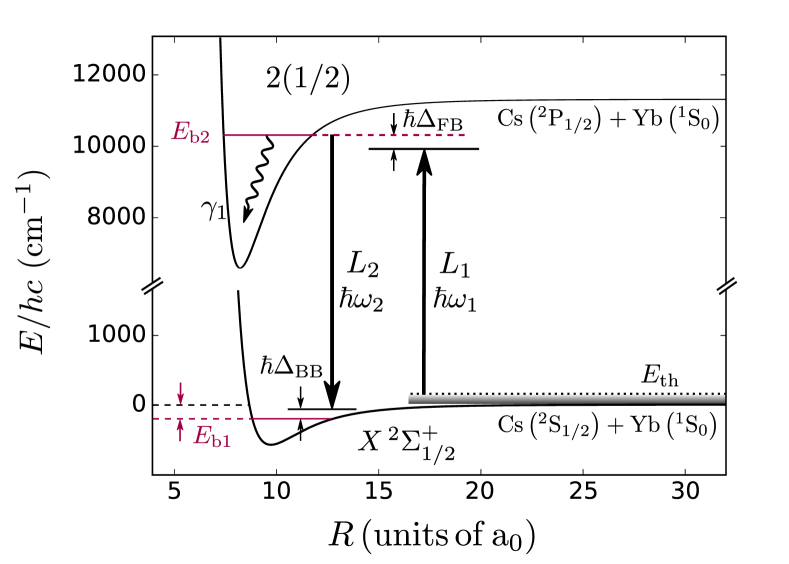
Figure 1: Two-photon photoassociation for the measurement of the binding energy, $E_{\rm b1}$, of a vibrational level of CsYb in its electronic ground state. A pair of colliding Cs and Yb atoms with thermal energy $E_{\rm th}$ is associated to form a CsYb molecule in a rovibrational level of the electronically excited $2(1/2)$ state by light of frequency $\omega_{1}$. This rovibrational level is coupled to a level in the electronic ground state, $X\,^{2}\Sigma^{+}_{1/2}$, by light of frequency $\omega_{2}$. The molecular curves plotted here are adapted from Ref. Meniailava and Shundalau (2017). The internuclear distances where the transitions occur are not shown to scale.

II.1 Overview

The two-photon photoassociation process is shown in Fig. 1. This scheme is an extension of one-photon photoassociation Bohn and Julienne (1999); Jones et al. (2006), whereby a pair of colliding atoms is associated to form a molecule in a rovibrational level of an electronically excited molecular state. The laser that drives the one-photon photoassociation, $L_{1}$, has frequency $\omega_{1}$ and intensity $I_{1}$; it is detuned from a free-bound transition by $\Delta_{\rm FB}$. The second laser, $L_{2}$, has frequency $\omega_{2}$ and intensity $I_{2}$; it couples the electronically excited molecule to a rovibrational level of the molecule in the electronic ground state. Its detuning from this bound-bound transition is $\Delta_{\rm BB}$. When $L_{2}$ is resonant with a bound-bound transition, the coupling leads to the formation of a dark state and the suppression of the absorption of $L_{1}$. Such two-photon dark resonances can be used to measure the binding energies, $E_{\rm b1}$, of vibrational levels of the molecule in the electronic ground state. In the undressed, zero-temperature limit, the binding energy is given simply by the difference in photon energy of the two lasers, $E_{\rm b1}=\hbar\left(\omega_{2}-\omega_{1}\right)$, when on two-photon resonance. This technique has been applied in a large number of single-species Abraham et al. (1996); Tsai et al. (1997); van Abeelen and Verhaar (1999); Wang et al. (2000); Vanhaecke et al. (2004); Moal et al. (2006); Martinez de Escobar et al. (2008); Kitagawa et al. (2008); Gunton et al. (2013); Pachomow et al. (2017) and two-species ultracold atom experiments Ni et al. (2008); Münchow et al. (2011); Debatin et al. (2011); Guo et al. (2017); Dutta et al. (2017); Rvachov et al. (2018) with considerable success.

For the specific case of CsYb discussed in this paper, the first photon excites the colliding atoms into a rovibrational level of the molecule close to the Cs(${}^{2}P_{1/2}$) + Yb(${}^{1}S_{0}$) asymptote. The electronic state at this threshold is designated 2(1/2) to indicate that it is the second (first excited) state with total electronic angular momentum $\Omega=1/2$ about the internuclear axis. It correlates at short range with the $1\,^{2}\Pi_{1/2}$ electronic state in Hund’s case (a) notation Meniailava and Shundalau (2017), but at long range the $1\,^{2}\Pi_{1/2}$ and $2\,^{2}\Sigma_{1/2}$ states are strongly mixed by spin-orbit coupling. We have recently reported photoassociation spectroscopy of the vibrational levels of the molecule within 500 GHz of the 2(1/2) threshold Guttridge et al. (2018). In this work we add a second photon to couple the vibrational level in the electronically excited state to a near-threshold level of the $X\,^{2}\Sigma^{+}_{1/2}$ electronic ground state. We label each vibrational level by its vibrational number $n$ below the associated threshold, such that $n=-1$ corresponds to the least-bound state, using $n^{\prime}$ for the electronically excited state and $n^{\prime\prime}$ for the ground state. Because of the low temperature of our atomic mixtures, combined with the selection rule $\Delta N=0$, all the rovibrational levels we measure have rotational quantum number $N=0$.

II.2 Experimental Setup

The experimental setup has been described in the context of our previous work Kemp et al. (2016); Hopkins et al. (2016); Guttridge et al. (2016, 2017, 2018). Here we focus on details of the ultracold atomic mixtures and the two-photon photoassociation setup.

Our measurements are performed on mixtures of Cs and Yb confined in an optical dipole trap (ODT). The ODT is formed from the output of a broadband fiber laser (IPG YLR-100-LP) with a wavelength of $1070(3)\,$nm and consists of two beams crossed at an angle of $40^{\circ}$ with waists of $33(4)\,\mu$m and $72(4)\,\mu$m. The measured Yb(Cs) trap frequencies are $240(750)\,$Hz radially and $40(120)\,$Hz axially. The trap depths for the two species are $U_{\mathrm{Yb}}=5\,\mu$K and $U_{\mathrm{Cs}}=85\,\mu$K respectively. We load the ODT with a mixture of $7\times 10^{4}$ Cs atoms at $T_{\mathrm{Cs}}=6\,\mu$K in the absolute ground state $6^{2}S_{1/2}$ $\ket{F=3,m_{F}=+3}$ and Yb atoms at $T_{\mathrm{Yb}}=1\,\mu$K in the ${}^{1}S_{0}$ ground state. The number of Yb atoms depends on the Yb isotope involved. Typically, we use $8\times 10^{5}$ atoms for ¹⁷⁴Yb, $4\times 10^{5}$ atoms for ¹⁷⁰Yb or $3\times 10^{5}$ atoms for ¹⁷³Yb. For both atomic species the atom number is measured using resonant absorption imaging after a short time of flight.

The light for two-photon photoassociation is derived from two independent lasers. $L_{1}$ is a Ti:Sapphire laser (M Squared SolsTiS) and $L_{2}$ is a Distributed Bragg Reflector (DBR) laser. Both lasers are frequency-stabilized using a high-finesse optical cavity, the length of which is stabilized to a Cs atomic transition using the Pound-Drever-Hall method Drever et al. (1983). The light sent to the optical cavity from $L_{1}$ and $L_{2}$ is first passed through two independent broadband fiber electro-optic modulators (EOMs) (EOSPACE PM-0S5-10-PFA-PFA-895) to add frequency sidebands. We then utilize the ‘electronic sideband’ technique Thorpe et al. (2008); Gregory et al. (2015) to allow continuous tuning of the two laser frequencies; by stabilizing a frequency sideband to a cavity transmission peak, the carrier frequencies of both lasers may be tuned over the $748.852(5)\,$MHz free spectral range (FSR) of the cavity by changing the modulation frequencies applied to the EOMs. By stabilizing the two lasers to different modes of the cavity we can control their frequency difference, $\omega_{1}-\omega_{2}$, over many GHz.

The main outputs of lasers $L_{1}$ and $L_{2}$ are overlapped, transmitted through an acousto-optic modulator for fast intensity control and coupled into a fiber that carries the light to the experiment. The output of the fiber is focused onto the atomic mixture with a waist of $150\,\mu$m and is circularly polarized to drive $\sigma^{+}$ transitions. This polarization gives us the strongest two-photon transitions from the Cs($6^{2}S_{1/2}F=3,m_{F}=+3$) + Yb(${}^{1}S_{0}$) scattering state to the $F=3$ manifold of the molecular electronic ground state via an intermediate vibrational level of CsYb in the $F^{\prime}=4$ manifold of the $2(1/2)$ excited state Guttridge et al. (2018).

We measure the frequency difference between lasers $L_{1}$ and $L_{2}$ using one of three methods, depending on the binding energy of the state under investigation. Most generally, the frequency difference is determined from the difference in the modulation frequencies applied to the two EOMs, combined with the number of cavity FSRs between the two modes used for frequency stabilization. Light from both lasers is coupled into a commercial wavemeter (Bristol 671A) for absolute frequency calibration and unambiguous determination of the cavity mode. For binding energies below 2 GHz, the frequency difference between the two lasers is measured directly from the beat frequency recorded on a fast photodiode (EOT ET-2030A). In the special case of the least-bound state, we do not use DBR laser and instead we drive the AOM with two RF frequencies. Generating the two-photon detuning in this way eliminates any effects of laser frequency noise and allows a very precise determination of the frequency difference.

II.3 Experimental Results

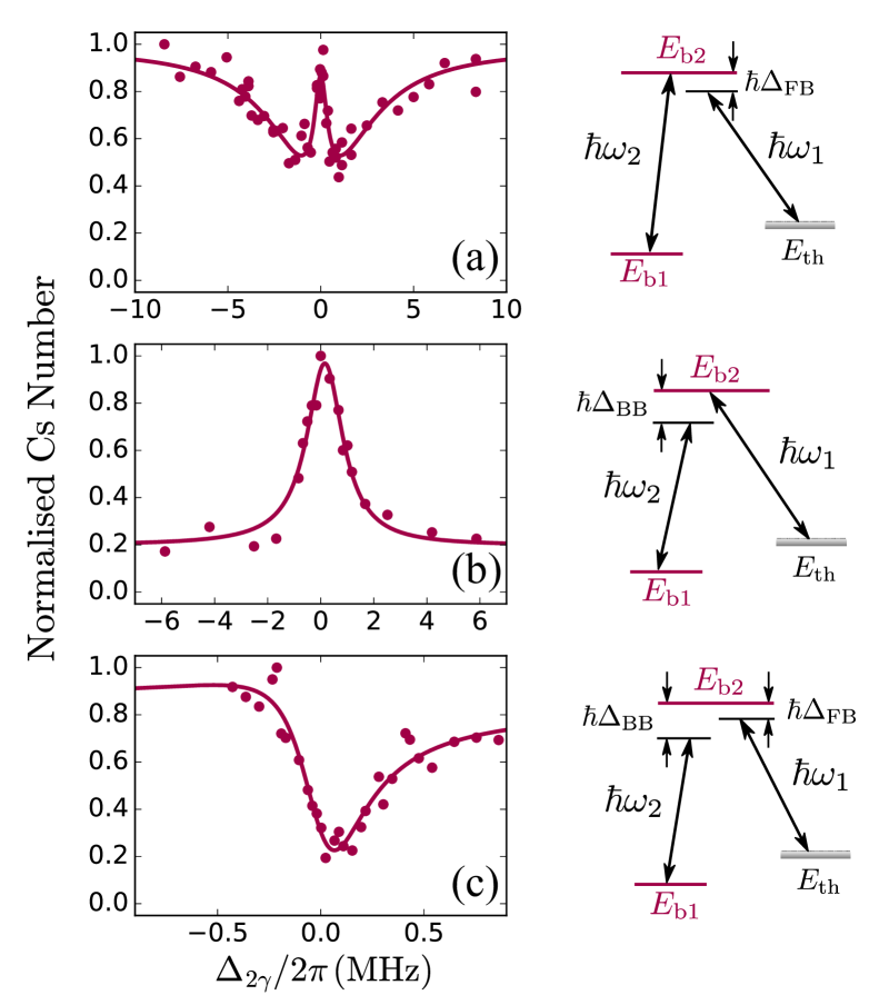
Figure 2: Measurement of the least-bound state of Cs¹⁷⁴Yb in the $X\,^{2}\Sigma^{+}_{1/2}$ electronic ground state by two-photon photoassociation spectroscopy. The intermediate state used is the $n^{\prime}=-13$ level of the molecule in the $2(1/2)$ state. Left panel: Two-photon photoassociation spectra. Normalized number of Cs atoms plotted against $\Delta_{2\gamma}=\Delta_{\mathrm{FB}}-\Delta_{\mathrm{BB}}$. Right panel: Simplified level structure for the two-photon photoassociation transitions. (a) Dark-resonance spectroscopy performed by scanning $\omega_{1}$. The red solid line shows a fit using Eq. 1, the analytical solution of the optical Bloch equations for a lambda-type three-level system. The best-fit parameters are $\Omega_{\rm BB}/2\pi=2(1)$ MHz, $\Gamma/2\pi=6(1)$ MHz and $\Gamma_{\rm eff}/2\pi=2(1)\times 10^{2}$ kHz. (b) Dark-resonance spectroscopy performed by scanning $\omega_{2}$. The red solid line shows a fit using a Lorentzian profile. (c) Raman spectroscopy. The red solid line shows a fit using a Fano profile. The spectra shown in (a),(b),(c) were obtained with laser intensities $I_{1}=0.42,0.68,1.1\,{\rm W/cm^{2}}$ and $I_{2}=0.79,0.57,0.76\,{\rm W/cm^{2}}$, respectively.

Two-photon photoassociation measurements are performed by illuminating the atomic mixture with light from lasers $L_{1}$ and $L_{2}$ for a variable time up to $250\,$ms, in a magnetic field of 2.2(2) G. Figure 2 shows the two-photon feature for the least-bound $n^{\prime\prime}=-1$ level of Cs¹⁷⁴Yb, using the $n^{\prime}=-13$ level of the 2(1/2) state as the intermediate state. We detect the two-photon resonance by measuring the number of Cs atoms remaining after exposure to the photoassociation light as a function of the two-photon detuning $\Delta_{2\gamma}=\Delta_{\rm FB}-\Delta_{\mathrm{BB}}$. Three different lineshapes may be observed, depending on the relative intensities and detunings of the lasers.

Figure 2(a) shows the lineshape observed using two-photon dark-resonance spectroscopy Winkler et al. (2005); Debatin et al. (2011). In this method $\omega_{2}$ is fixed on resonance with the bound-bound transition ($\Delta_{\mathrm{BB}}=0$) and $\omega_{1}$ is scanned over the free-bound transition. The spectrum exhibits the w-shaped profile expected for electromagnetically induced transparency (EIT) in a lambda-type three-level system Fleischhauer et al. (2005) and we therefore refer to this as the EIT lineshape. In the wings we observe a Lorentzian profile originating from one-photon photoassociation to the $n^{\prime}=-13$ level of the 2(1/2) state. Then, on resonance we see a suppression of the photoassociative loss due to the creation of a dark state composed of the initial atomic scattering state and the molecular ground state. This dark state is decoupled from the intermediate $n^{\prime}=-13$ state and leads to the observed ‘transparency’. We fit the data with the analytical solution of the optical Bloch equations for a lambda-type three-level system Fleischhauer et al. (2005); Debatin et al. (2011) in the limit of $\Omega_{\rm FB}\ll\Omega_{\rm BB}$,

$$\frac{N}{N_{0}}=\exp\left(-\frac{t_{\mathrm{PA}}\Omega_{\mathrm{FB}}^{2}(4\Gamma\Delta_{2\gamma}^{2}+\Gamma_{\mathrm{eff}}(\Omega_{\mathrm{BB}}^{2}+\Gamma_{\mathrm{eff}}\Gamma))}{|\Omega_{\mathrm{BB}}^{2}+(\Gamma+2i\Delta_{\rm FB})(\Gamma_{\mathrm{eff}}+2i\Delta_{2\gamma})|^{2}}\right).$$ (1)

Here, $t_{\mathrm{PA}}$ is the irradiation time of the photoassociation lasers, $\Omega_{\mathrm{FB}}$ $(\Omega_{\mathrm{BB}})$ is the Rabi frequency on the free-bound (bound-bound) transition, $\Delta_{2\gamma}$ is the detuning from two-photon resonance, $\Gamma$ is the power-broadened linewidth of the free-bound transition and $\Gamma_{\mathrm{eff}}$ is a phenomenological constant that accounts for the decoherence of the dark state.

Figure 2(b) shows the dark-resonance spectrum observed when $\omega_{1}$ is resonant with the free-bound transition $(\Delta_{\mathrm{FB}}=0)$ and $\omega_{2}$ is scanned. This complements the EIT lineshape shown in Fig. 2(a); the only difference is which laser frequency is scanned. Off resonance with the bound-bound transition, we observe a large loss of Cs atoms due to the production of Cs*Yb molecules . When $L_{2}$ is tuned close to resonance with the bound-bound transition, the photon-dressed ground state and the excited state couple to form two dressed states Fleischhauer et al. (2005). The splitting of the dressed states creates a dark state where $L_{1}$ is no longer resonant with the free-bound transition. Therefore, the production of Cs*Yb molecules is suppressed and there is a recovery in the Cs number. In the perturbative limit, Eq. 1 reduces to a Lorentzian profile with a width proportional to $\Omega_{\rm BB}^{2}$ and we therefore fit the data with a Lorenztian lineshape. This dark-resonance technique is the simplest method for the observation of a two-photon resonance, as with sufficient $L_{2}$ intensity the feature can be significantly broadened without shifting the line center. However, the background number of Cs atoms is sensitive to the one-photon photoassociation loss rate and can therefore drift in response to changes in the Yb density, the Cs density, or the photoassociation light intensity or polarization.

Figure 2(c) shows an alternative method for observing the two-photon resonance using Raman spectroscopy. In this case, $\omega_{1}$ is detuned from the free-bound transition ($\Delta_{\mathrm{FB}}=-15\,\mathrm{MHz}$) and $L_{2}$ drives a stimulated Raman transition to a vibrational level of the electronic ground state when the Raman condition is fulfilled ($\Delta_{\mathrm{FB}}=\Delta_{\mathrm{BB}}$). This gives a narrow lineshape. The creation of a ground-state CsYb molecule, which is dark to our imaging, causes a decrease in the number of observed Cs atoms. The asymmetric lineshape originates from the interference between the two paths $(E_{\rm th}\rightarrow E_{\rm b_{2}}$ and $E_{\rm th}\rightarrow E_{\rm b_{2}}\rightarrow E_{\rm b_{1}}\rightarrow E_{\rm b_{2}})$ Bohn and Julienne (1996); Portier et al. (2009) and incorporates a Fano profile Fano (1961).

We use Raman spectroscopy as the primary method for the observation of $n^{\prime\prime}=-1$ levels, as the lineshape of the two-photon feature is narrow for low powers of $L_{1}$ and $L_{2}$. However, coupling of the ground and excited states by $L_{1}$ and $L_{2}$ causes light shifts in both levels that are linear in laser intensity in the perturbative limit Portier et al. (2009). Figure 3 shows the shifts $\delta_{1}(I_{1})$ and $\delta_{2}(I_{2})$ of the two-photon resonance position as functions of the intensities of lasers $L_{1}$ and $L_{2}$. We fit a straight line to the data to extract the line position at zero intensity. As expected, the gradient of the shift with respect to intensity is larger for the bound-bound transition, due to the larger Franck-Condon factor (FCF) between two bound states than between a bound state and a scattering state.

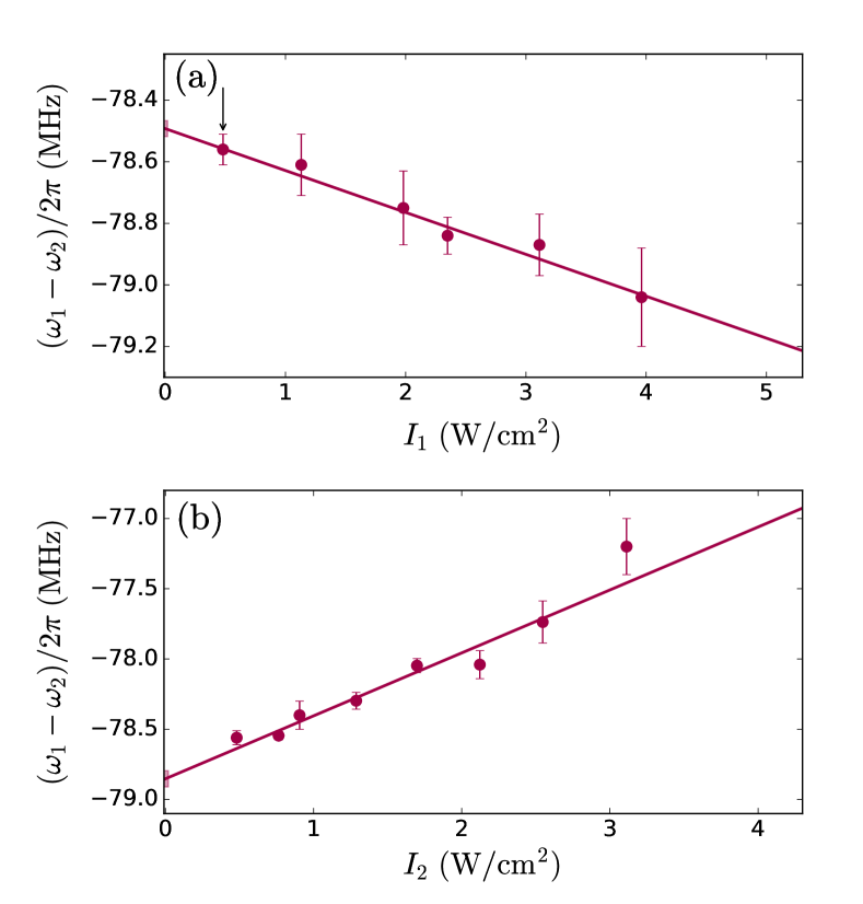
Figure 3: Light shift of the Cs¹⁷⁴Yb $n^{\prime\prime}=-1$ Raman line as a function of photoassociation laser intensity, using the $n^{\prime}=-13$ intermediate state. (a) Measured line center frequency as a function of intensity $I_{1}$ of laser $L_{1}$ driving the free-bound transition. The intensity of laser $L_{2}$ for this data set was $I_{2}=0.35\,{\rm W/cm^{2}}$. (b) Measured line center frequency as a function of intensity $I_{2}$ of laser $L_{2}$ driving the bound-bound transition. The intensity of laser $L_{1}$ for this data set was $I_{1}=0.48\,{\rm W/cm^{2}}$ and is highlighted in (a). The $1\sigma$ uncertainties in the intercepts are represented by the shaded regions at the origins.

Further systematic effects that may shift the position of the Raman line are the ac Stark shift due to the dipole trapping light, the Zeeman effect due to the magnetic field and the finite energy of the initial atomic collision. The trapping light may systematically shift the line position by a differential ac Stark shift between the atomic pair and the molecular state $E_{\rm b1}$. However, this shift is expected to be small for the weakly bound states considered here. The effect of magnetic field on the results is small, as the linear Zeeman shift is almost the same for the atomic state and the molecular state. Investigation of shifts due to both magnetic field and dipole trap intensity found no significant shift at the resolution of the measurements ($<100\,$kHz). The remaining systematic shift is the thermal shift, $E_{\rm th}$, due to the energy of the initial collision between the Cs and Yb atoms. We account for this by subtracting the mean collision energy $E_{\rm th}=\frac{3}{2}\mu k_{\rm B}\left(T_{\rm Yb}/m_{\rm Yb}+T_{\rm Cs}/m_{\rm Cs}\right)$, where $\mu$ is the reduced mass. For our initial temperatures of $T_{\rm Yb}=1\,\mu$K and $T_{\rm Cs}=6\,\mu$K, the correction is of order $100\,$kHz and is insignificant except for the measurements of the $n^{\prime\prime}=-1$ levels.

Yb	$n^{\prime}$	$n^{\prime\prime}$	$E_{\rm b1}/h$ (MHz)
Isotope			Obs	Uncertainty	Calc	Obs$-$Calc
170	-15	-1	15.7	0.3	15.6	0.1
170	-15	-3	1576	2	1576	0
170	-15	-4	4259	2	4257	2
170	-15	-5	8988	2	8989	1
173	-13	-1	56.8	0.2	57.0	0.2
173	-13	-2	592	1	591	1
173	-13	-3	2166	1	2165	1
174	-13	-1	78.66	0.09	78.73	0.07
174	-17	-1	78.7	0.1	78.7	0.0
174	-17	-2	686.4	0.7	686.5	0.1
174	-17	-3	2385.5	0.9	2384.5	1
174	-17	-4	5749	1	5747	2
174	-17	-5	11358	1	11359	1
174	-17	-6	19803	1	19805	2
174	-17	-7	31672	2	31668	4

Table 1: Observed binding energies and their uncertainties for vibrational levels of three different isotopologs of CsYb in its electronic ground state, together with experimental $1\sigma$ uncertainties and binding energies calculated from the fitted interaction potential.

In total we observed 14 ground-state vibrational levels for the three isotopologs Cs¹⁷⁰Yb, Cs¹⁷³Yb and Cs¹⁷⁴Yb. The binding energies of these levels, corrected for thermal shifts and light shifts due to $L_{1}$ and $L_{2}$, are listed in Table 1. The dark-resonance spectroscopy method scanning $\omega_{2}$ was used for measurements of the $n^{\prime\prime}<-1$ levels. The smaller error bars for the $n^{\prime\prime}=-1$ levels result from the narrower Raman feature and the different method of generating the small frequency offset between the two photons. Frequency instabilities due to beating between the sidebands of $L_{1}$ and $L_{2}$ prevented observation of the $n^{\prime\prime}=-2$ state of Cs¹⁷⁰Yb. The $n^{\prime\prime}=-1$ level of Cs¹⁷⁴Yb was measured with both $n^{\prime}=-13$ and $n^{\prime}=-17$ as intermediate states to verify that the measurements are of the ground electronic state and not two-photon transitions to a higher-energy electronic state. We chose to use intermediate states with moderately large binding energies to increase the detuning of the photoassociation light from the Cs $D_{1}$ transition; a greater feature depth is observed for larger detuning due to the reduction of off-resonant Cs losses Guttridge et al. (2018).

III Line strengths & Autler-Townes Spectroscopy

The strengths of transitions between the electronically excited state and ground state may be determined from the light shift of the Raman spectroscopy measurements. The systematic dependencies of Raman transitions in three-level lambda-type systems have been studied extensively Brewer and Hahn (1975); Orriols (1979); Lounis and Cohen-Tannoudji (1992); Bohn and Julienne (1996); Zanon-Willette et al. (2011). For atomic systems it has been shown that the light shift is proportional to $\Omega^{2}$, where $\Omega$ is the Rabi frequency associated with either one-photon transition Brewer and Hahn (1975); Orriols (1979). Investigations of molecular systems have found that the light shift of the resonance maintains this $\Omega^{2}$ dependence even in the presence of decay out of the three-level system Portier et al. (2009); Cohen-Tannoudji (2015). Here we determine the line strengths for the bound-bound transitions given by $\Omega_{\rm BB}^{2}/I_{2}$ using light-shift measurements of the type presented in Fig. 3(b).

For the Raman lineshape shown in Fig. 2(c), the maximum loss of Cs atoms occurs at a two-photon detuning $\omega_{1}-\omega_{2}=E_{\rm b1}/\hbar+\delta_{1}(I_{1})+\delta_{2}(I_{2})$. Here $\delta_{1}(I_{1})$ and $\delta_{2}(I_{2})$ are the light shifts of the transition and Portier et al. (2009)

$$\frac{\delta_{2}(I_{2})}{I_{2}}=\left(\frac{\Omega_{\rm BB}^{2}/I_{2}}{4\Delta_{\rm FB}^{2}+\Gamma^{2}}\right)\Delta_{\rm FB},$$ (2)

where $\Delta_{\rm FB}\simeq\Delta_{\rm BB}$ in the vicinity of the Raman resonance . It follows that the line strength $\Omega_{\rm BB}^{2}/I_{2}$ may be obtained from the gradient of resonance position with respect to intensity $I_{2}$ using Eq. 2. The results for the measured line strengths of $n^{\prime}=-17\rightarrow n^{\prime\prime}$ transitions in Cs¹⁷⁴Yb are presented in Fig. 4 as green open circles.

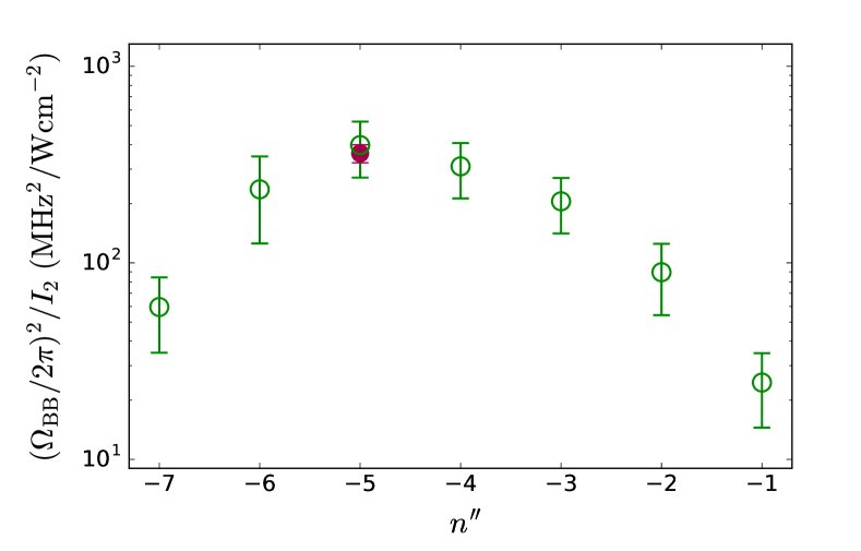
Figure 4: Measured line strengths of $n^{\prime}=-17\rightarrow n^{\prime\prime}$ transitions in Cs¹⁷⁴Yb. The line strength $\Omega_{\rm BB}^{2}/I_{2}$ is plotted as a function of ground-state vibrational level $n^{\prime\prime}$. Green open circles represent measurements of the Rabi frequencies from the line shifts of the Raman loss features. The filled red circle represents the measurement of the $n^{\prime}=-17\rightarrow n^{\prime\prime}=-5$ transition using Autler-Townes spectroscopy.

The line strengths of the bound-bound transitions may also be determined using Autler-Townes spectroscopy (ATS) to measure the Rabi frequency, $\Omega_{\rm BB}$, directly from the splitting of the two dressed states. The experimental configuration for ATS is the same as in Fig. 2(a), but instead of measuring the binding energy we measure the splitting of the dressed states as a function of the intensity of $L_{2}$. Figure 5 shows the Autler-Townes spectrum of the $n^{\prime}=-17\rightarrow n^{\prime\prime}=-5$ transition in Cs¹⁷⁴Yb. In the figure, $\omega_{2}$ is fixed on resonance ($\Delta_{\rm BB}=0$) and $\omega_{1}$ is scanned over the free-bound $n^{\prime}=-17$ transition for a number of different intensities of $L_{2}$. The Autler-Townes splitting of the one-photon line is clearly visible as the intensity of the bound-bound laser is increased. The Rabi frequency $\Omega_{\rm BB}$ is extracted by fitting Eq. 1 to the data, and is approximately the splitting of the two peaks as labeled in the figure. The quantity of interest, $\Omega_{\rm BB}/\sqrt{I_{2}}$, is then extracted from a linear fit as shown in Fig. 5(b). We find that, for the $n^{\prime}=-17\rightarrow n^{\prime\prime}=-5$ transition, $\Omega_{\rm BB}/\sqrt{I_{2}}=2\pi\times 19(1)\,\mathrm{MHz}{/}\sqrt{\mathrm{W\,cm^{-2}}}$. We include this measurement in Fig. 4 as the red closed circle. We did not measure all the transitions using ATS due to the $\sim 30$ s load-detection cycle associated with conducting the measurements. Nevertheless, the excellent agreement between the two measurements of the line strength for the $n^{\prime}=-17\rightarrow n^{\prime\prime}=-5$ transition confirms the validity of using the light-shift measurements.

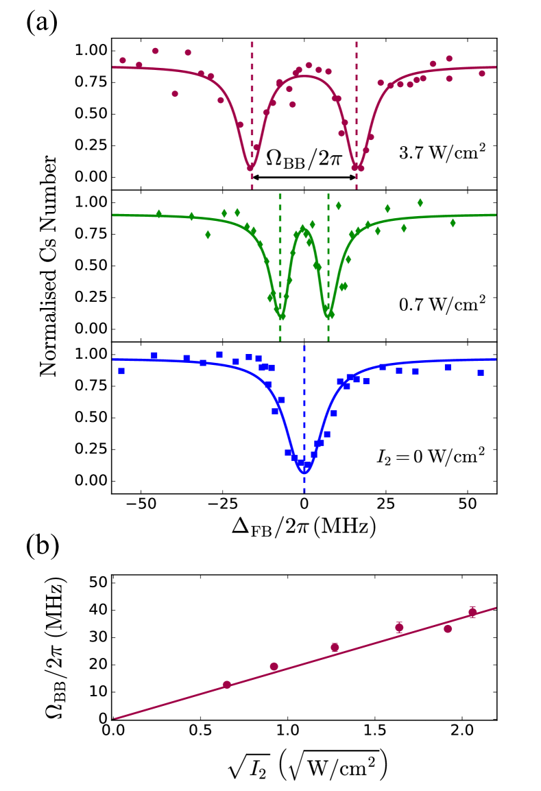
Figure 5: Autler-Townes spectroscopy (ATS) of the $n^{\prime}=-17\rightarrow n^{\prime\prime}=-5$ transition in Cs¹⁷⁴Yb. (a) Normalized Cs number versus detuning, $\Delta_{\rm FB}$, of laser $L_{1}$ from the $n^{\prime}=-17$ free-bound transition. The second laser $L_{2}$ is on resonance with the bound-bound transition, $\Delta_{\rm BB}=0$, and the splitting of the one-photon lineshape is observed for varying intensities $I_{2}$ of laser $L_{2}$. (b) Bound-bound Rabi frequency $\Omega_{\rm BB}$ extracted from the ATS measurements as a function of the square root of the intensity $I_{2}$ of laser $L_{2}$ that drives the bound-bound transition. The solid line is a linear fit with the intercept constrained to be zero.

The FCFs that determine the line strengths are dominated by the region around the outermost lobe of the wavefunction for $n^{\prime}=-17$. This is far inside the outer turning points of the near-threshold levels of the ground electronic state. In this region, the wave functions of the different near-threshold levels in the electronic ground state are almost in phase with one another, but with amplitudes proportional to $E_{\rm b1}^{1/3}$ Le Roy and Bernstein (1970) and line strengths proportional to $E_{\rm b1}^{2/3}$. However, the wave functions start to change phase as $E_{\rm b1}$ increases; eventually the phase difference between the wave functions in the two electronic states overcomes the amplitude factor and the FCF starts to decrease. Figure 4 shows that the peak line strength occurs around $n^{\prime\prime}=-5$ in the present case.

Ref. Guttridge et al. (2018) fitted the one-photon photoassociation spectra to a near-dissociation expansion. However, the quantities $C_{6}$ and $C_{8}$ resulting from this are effective dispersion coefficients that incorporate higher-order effects. They are not sufficient to determine the outer turning point accurately at the energy of the $n^{\prime}=-17$ level, which is bound by 286 GHz. Calculating FCFs will require a more complete model of the excited-state potential, which is beyond the scope of this paper.

IV Determination of the Interaction Potential

The spacings between near-threshold bound states are largely determined by the long-range potential

$$V(R)\sim\sum_{n=6,8,10,\dots}-C_{n}R^{-n}\quad(\hbox{as}\ R\to\infty),$$ (3)

where $C_{n}$ are dispersion coefficients. However, at least one additional parameter is needed to specify the actual positions of the levels. To the extent that the long-range potential is described by Eq. 3, only one such parameter is needed. This parameter may be thought of as the binding energy of the least-bound state, the scattering length, or the non-integer vibrational quantum number at dissociation. Physically, it is determined by the potential at short range, and is sometimes described as the “volume” of the potential well, as quantified by the WKB phase integral at dissociation

$$\Phi=\int^{\infty}_{R_{\rm in}}\sqrt{\frac{-2\mu}{\hbar^{2}}V(R)}\,dR,$$ (4)

where $R_{\rm in}$ is the inner turning point. For a single isotopolog, potentials with the same fractional part of $\Phi/\pi$ have the same near-threshold bound states (and the same scattering length), even if they have a different number of vibrational levels $N_{\rm vib}$. The Born-Oppenheimer potential $V(R)$ is independent of reduced mass $\mu$, but the dependence of $\Phi$ on $\mu$ means that potentials with different $N_{\rm vib}$ for one isotopolog imply different values of the fractional part of $\Phi/\pi$, and hence different level positions, for other isotopologs. Comparing measurements for different isotopologs can thus establish the number of vibrational levels supported by the potential.

Calculations of Feshbach resonance widths Żuchowski et al. (2010); Brue and Hutson (2013) require a complete interaction potential $V(R)$, rather than just the long-range form, Eq. 3. To obtain such a potential, we base the short-range part on electronic structure calculations. Interaction potentials for the ${}^{2}\Sigma$ ground state of CsYb have been calculated at various levels of electronic structure theory Meyer and Bohn (2009); Brue and Hutson (2013); Shao et al. (2017); Meniailava and Shundalau (2017). The potential is dominated by dispersion interactions, with little chemical bonding, due to the large difference in ionisation energies for Cs and Yb . We therefore choose to base our short-range potential on that of Brue and Hutson Brue and Hutson (2013), as the coupled-cluster methods and basis sets they used are likely to give a good description of the dispersion interactions.

The potential of Ref. Brue and Hutson (2013) has a well depth of $hc\times 620$ cm^-1 and supports 69 vibrational levels. In order to adjust this potential to fit our measured binding energies, we first represent it in an analytic form,

$$V(R)=Ae^{-\beta R}-\sum_{n=6,8,10}D_{n}(\beta R)C_{n}R^{-n}.$$ (5)

Here, $A$ and $\beta$ control the magnitude and range of the short-range repulsive wall of the potential and

$$D_{n}(\beta R)=1-e^{-\beta R}\sum_{m=0}^{n}\frac{(\beta R)^{m}}{m!}$$ (6)

is a Tang-Toennies damping function Tang and Toennies (1984). To reduce the number of free parameters, we use $C_{10}=(49/40)C_{8}^{2}/C_{6}$ as recommended by Thakkar and Smith Thakkar and Smith (1974). We fit the parameters $A$, $\beta$, $C_{6}$ and $C_{8}$ to the interaction energies from the electronic structure calculations of Ref. Brue and Hutson (2013). The functional form accurately represents the ab initio points, and the fit is not significantly improved by including an attractive exponential term; this confirms that there is little chemical bonding. The value of $C_{6}$ obtained in this way is 3800 $E_{\textrm{h}}a_{0}^{6}$, which is about 13% larger than the value of 3370 $E_{\textrm{h}}a_{0}^{6}$ obtained in Ref. Brue and Hutson (2013) using Tang’s combination rule Tang (1969). Here, $a_{0}$ is the Bohr radius and $E_{\textrm{h}}$ is the Hartree energy. This confirms that the electronic structure calculations of Ref. Brue and Hutson (2013) are adequate to give a qualitative (but not quantitative) description of the dispersion effects.

To fit the potential to the measured binding energies, we fit the dispersion coefficients $C_{6}$ and $C_{8}$, and vary $A$ to adjust the volume of the potential and thus the number of vibrational levels. We fix $\beta=0.83\,a_{0}^{-1}$ to the value obtained from fitting to the electronic structure calculations. These choices allow us to fit the aspects of the potential that are well determined by our measurements, using a small number of parameters, while maintaining a physically reasonable form for the entire potential.

Table 2: Fitted parameters and statistical uncertainties ($1\sigma$) from the least-squares fit to the binding energies. The sensitivity is as defined in Ref. Le Roy (1998).

Parameter	Value	Uncertainty	Sensitivity
$A/E_{\textrm{h}}$	13.8866515	0.2	$2\times 10^{-7}$
$C_{6}/E_{\textrm{h}}a_{0}^{6}$	3463.2060	4	$2\times 10^{-4}$
$C_{8}/E_{\textrm{h}}a_{0}^{8}$	502560.625	5000	$5\times 10^{-3}$

We calculate near-threshold bound states supported by the potential using the bound package Hutson (1993). The terms in the Hamiltonian that couple different electronic and nuclear spin channels (and cause Feshbach resonances) are very small Brue and Hutson (2013). The effective potential is thus almost identical for all spin channels. The bound molecular states are almost unaffected by these weak couplings. The effects of the atomic hyperfine splitting and Zeeman shifts are already accounted for in the measurement of the binding energies. We therefore calculate bound states using single-channel calculations, neglecting electron and nuclear spins and the effects of the magnetic field.

We carry out separate least-squares fits to the measured binding energies for each plausible number of vibrational levels $N_{\rm vib}$ . We fit to all three isotopologs simultaneously, using weights derived from the experimental uncertainties. We find the best fit for $N_{\rm vib}=77$ with a reduced chi-squared $\chi_{\nu}^{2}=1.3$. For $N_{\rm vib}=76$ and 78 we find $\chi_{\nu}^{2}=25$ and 26 respectively. The final fitted parameters are given in Table 2, with their uncertainties and sensitivities Le Roy (1998). As this is a very strongly correlated fit, rounding the fitted parameters to their uncertainties introduces very large errors in the calculated levels, so the parameters are given to a number of significant figures determined by their sensitivity Le Roy (1998) to allow accurate reproduction of the binding energies. The fitted value of $C_{6}$ is within 3% of the value from Tang’s combining rule Brue and Hutson (2013). The ground-state binding energies calculated from the fitted interaction potential are included in Table 1.

The statistical uncertainties in the potential parameters are very small. However, our model is somewhat restrictive, and the uncertainties in quantities derived from the potential are dominated by model dependence. To quantify this, we have explored a range of different models; these include using different values of $\beta$ and adding an attractive exponential term in the fit to the electronic structure calculations. The estimates of uncertainties due to model dependence given below are based on the variations observed in these tests. Further measurements of more deeply bound vibrational states would be necessary to determine the details of the short-range potential.

Table 3: Comparison of well depth and equilibrium distances of CsYb potentials. The uncertainties for the potential of the present work are dominated by model dependence, not statistics.

Ref.	$D_{\rm e}/hc$ (cm-1)	$R_{\rm e}\ (a_{0})$
This work	770(30)	9.25(50)
Brue and Hutson (2013)	621	9.72
Shao et al. (2017)	542	9.75
Meniailava and Shundalau (2017)	159	10.89
Meyer and Bohn (2009)	182	10.69

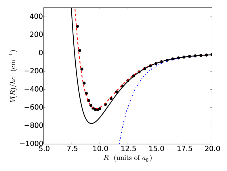
Figure 6: Potential curves for the $X~{}^{2}\Sigma_{1/2}^{+}$ ground state of CsYb. The dots are the electronic structure calculations of Ref. Brue and Hutson (2013); the red dashed line is the functional form Eq. (5) fitted to the electronic structure calculations; the solid black line is the final fitted potential; and the blue dash-dot line is the pure dispersion potential, Eq. (3), without a repulsive wall or dispersion damping functions.

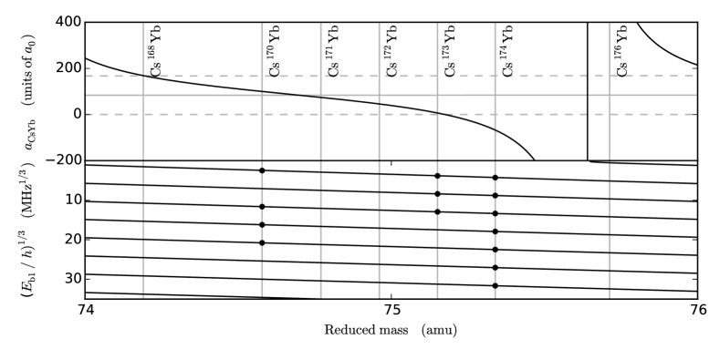
Figure 7: Interspecies scattering length (upper panel) and binding energies (lower panel) for CsYb as a function of reduced mass, calculated using the fitted interaction potential. Points show measured levels; error bars are smaller than the points on this scale. The vertical lines correspond to the stable Yb isotopes. The horizontal lines on the upper figure correspond to $a=0$, $\bar{a}$, and $2\bar{a}$.

Figure 6 shows the final fitted potential, along with the unmodified potential of Brue and Hutson Brue and Hutson (2013). The well depths $D_{\rm e}$ and equilibrium distances $R_{\rm e}$ for the ground-state potentials from Refs. Meyer and Bohn (2009), Brue and Hutson (2013), Meniailava and Shundalau (2017) and Shao et al. (2017) are compared with those for our fitted potential in Table 3. The minimum of our potential is deeper and at shorter range than any of those from electronic structure calculations, though comparable to those from Refs. Brue and Hutson (2013) and Shao et al. (2017). There is an inverse correlation between $D_{\rm e}$ and $R_{\rm e}$ for the different potentials from electronic structure calculations. Refs. Meyer and Bohn (2009) and Meniailava and Shundalau (2017) both used large-core effective core potentials for Yb, with only 2 active electrons; this might be responsible for their large equilibrium distances and small well depths, which are in poor agreement with the experimental results.

Table 4: Interspecies scattering lengths calculated from the fitted interaction potential. Both statistical uncertainties $(1\sigma)$ and estimated uncertainties from model dependence are given.

Mixture	$a\ (a_{0})$	Statistical	Model
		uncertainty $(a_{0})$	dependence $(a_{0})$
Cs+168Yb	165.98	0.15	0.4
Cs+170Yb	96.24	0.08	0.2
Cs+171Yb	69.99	0.08	0.3
Cs+172Yb	41.03	0.12	0.5
Cs+173Yb	1.0	0.2	1.0
Cs+174Yb	$-74.8$	0.5	3
Cs+176Yb	798	7	40

V Prediction of scattering lengths

We have used our fitted potential to predict interspecies scattering lengths for all isotope combinations of Cs+Yb. These are given in Table 4. In this case the uncertainties from statistics and model dependence are comparable, though the latter are larger. The scattering lengths are also shown as a function of reduced mass in Fig. 7, along with both observed and calculated binding energies. The cube root of the binding energy varies almost linearly with reduced mass for an interaction potential with $-C_{6}/R^{6}$ long-range behavior Le Roy and Bernstein (1970), except for a small curvature very near dissociation due to the Gribakin-Flambaum correction Gribakin and Flambaum (1993) of $\pi/8$ to the WKB quantization condition at threshold.

The scattering lengths are in remarkably good agreement with our previous estimates based on interspecies thermalization Guttridge et al. (2017). Six of the isotope combinations have scattering lengths between $-2\bar{a}$ and $2\bar{a}$, where $\bar{a}$ is the mean scattering length of Gribakin and Flambaum Gribakin and Flambaum (1993). The exception is Cs+¹⁷⁶Yb, which has a very large scattering length due to the presence of an additional vibrational level just below threshold. The moderate values of the scattering length for four of the bosonic Yb isotopes should allow the production of miscible two-species condensates Riboli and Modugno (2002) with Cs at the magnetic field required to minimize the Cs three-body loss rate Weber et al. (2003). Conversely, the large positive scattering length for Cs+¹⁷⁶Yb is likely to result in an enhancement of the widths of Feshbach resonances Brue and Hutson (2013). The negative interspecies scattering length for Cs+¹⁷⁴Yb opens up the intriguing prospect of forming self-bound quantum droplets Petrov (2015); Cabrera et al. (2018); Cheiney et al. (2018). The very small interspecies scattering length of Cs+¹⁷³Yb indicates that the degenerate Bose-Fermi mixture would be essentially non-interacting. In contrast, the scattering length of $70\,a_{0}$ for Cs+¹⁷¹Yb is ideal for sympathetic cooling of ¹⁷¹Yb to degeneracy Taie et al. (2010); Vaidya et al. (2015), overcoming the problem of the small intraspecies scattering length Kitagawa et al. (2008) that makes direct evaporative cooling ineffective.

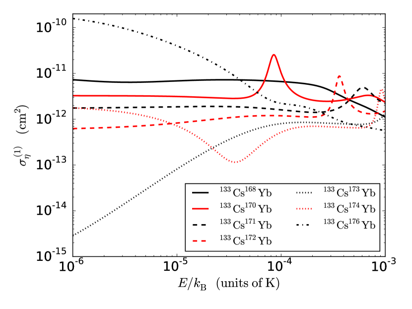
Figure 8: Calculated cross sections for interspecies thermalization of Cs with Yb, as a function of collision energy $E$.

Figure 8 shows the cross sections $\sigma_{\eta}^{(1)}$ that characterize interspecies thermalization Frye and Hutson (2014), as a function of collision energy, for all the isotopic combinations. These are obtained from single-channel quantum scattering calculations on the fitted interaction potential, using the molscat package Hutson and Green (1994) and the post-processor sbe Hutson and Green (1982), including all relevant partial waves. The low-energy cross sections vary across more than 4 orders of magnitude. Cs+¹⁷³Yb has a very small cross section at low energy, due to its tiny zero-energy scattering length, but this increases rapidly with energy due to both effective-range effects and p-wave scattering. Cs+¹⁷⁴Yb has a negative scattering length at zero energy, and exhibits a Ramsauer-Townsend minimum near 30 $\mu$K, where the energy-dependent scattering length crosses zero. However, the minimum is not particularly deep, because 30 $\mu$K is high enough that the p-wave contributions are significant. Cs+¹⁷⁰Yb exhibits a d-wave shape resonance around 90 $\mu$K, while Cs+¹⁷¹Yb and Cs+¹⁷²Yb exhibit f-wave shape resonances around 600 $\mu$K and 400 $\mu$K, respectively. Cs+¹⁷³Yb and Cs+¹⁷⁴Yb exhibit g-wave shape resonances at even higher energies.

VI Conclusion

We have used two-photon photoassociation spectroscopy to measure the binding energies of vibrational levels of the electronic ground state of the heteronuclear CsYb molecule. We measure the binding energy of vibrational levels for three isotopologs of CsYb. This is sufficient to establish that the ground state supports 77 vibrational levels. We fit a ground-state interaction potential based on electronic structure calculations to the binding energies for all the isotopologs together. Using our optimized potential, we calculate values of the s-wave scattering length for all 7 isotopic combinations of ¹³³Cs and Yb. The results are very promising for the sympathetic cooling of ¹⁷¹Yb and for the production of quantum-degenerate mixtures.

The fitted interaction potential may be used to predict positions and widths of interspecies Feshbach resonances between a closed-shell atom and an alkali atom Żuchowski et al. (2010); Brue and Hutson (2013); Barbé et al. (2018). Magnetoassociation using these predicted Feshbach resonances, followed by STIRAP Bergmann et al. (1998), is a promising route to the creation of ultracold ground-state ${}^{2}\Sigma$ molecules.