Refractors in anisotropic media
associated with norms

Abstract.

We show existence of interfaces between two anisotropic materials so that light is refracted in accordance with a given pattern of energy. To do this we formulate a vector Snell law for anisotropic media when the wave fronts are given by norms for which the corresponding unit spheres are strictly convex.

1. Introduction

Anisotropic materials are those whose optical properties vary according to the direction of propagation of light. Typical examples are crystals, where the refractive index depends on the direction of the incident light, see [BW59, Chapter XV], [LL84, Chapter XI] and [Som54, Chapter IV]. Important research was done on this subject because of it multiple applications, see the fundamental work [KK65], and [YY84], [Sch07] for more recent applications and references. Mathematically, in these materials wave fronts satisfy the Fresnel partial differential equation which in the particular case of isotropic materials is the eikonal equation. A difficulty with anisotropic materials in the geometrical optics regime is that incident rays may be refracted into two rays: an ordinary ray and an extraordinary ray. This is the phenomenon of bi-refringence, observed experimentally in crystals, and is a consequence from the fact that the Fresnel equation splits in general as the product of two surfaces, see (6.8).

The main purpose of this paper is to show existence of interfaces between two homogenous and anisotropic materials so that light is refracted in accordance with a given pattern of energy. As a main step to achieve this, we give a formulation of a vector Snell’s law in anisotropic materials when the wave fronts are given by norms in ${\mathbb{R}}^{n}$ which has independent interest. More precisely, suppose $N_{i}(x)$, $i=1,2$, are norms in ${\mathbb{R}}^{n}$, $\Sigma_{i}=\{x:N_{i}(x)=1\}$, $\Omega_{i}\subset\Sigma_{i}$ are domains, $f>0$ is an integrable function on $\Omega_{1}$, and $\mu$ is a Radon measure in $\Omega_{2}$ with $\int_{\Omega_{1}}f(x)\,dx=\mu(\Omega_{2})$. We have two anisotropic media $I$ and $II$ such that the wave fronts in $I$ are given by $N_{1}$ and the wave fronts in $II$ given by $N_{2}$. Light rays emanate from the origin, located in medium $I$, with intensity $f(x)$ for each $x\in\Omega_{1}$. We seek a surface $\mathcal{S}$ separating media $I$ and $II$ so that all rays emanating from the origin and with directions in $\Omega_{1}$ are refracted into rays with directions in $\Omega_{2}$ and the conservation of energy condition

$$\int_{\tau(E)}f(x)\,dx=\mu(E)$$

holds for each Borel set $E\subset\Omega_{2}$ where $\tau(E)=\{x\in\Omega_{1}:\text{$x$ is refracted into $E$}\}$. This is called the refractor problem, and when media $I$ and $II$ are homogeneous and isotropic it is solved in [GH09] using optimal mass transport and in [Gut14] with a different method. A main difficulty to solve this problem is to lay down the mathematical formulation of the physical laws and constraints in anisotropic media to our setting with norms.

To place our results in perspective we mention the following. A similar problem for norms but for reflection was studied in [CH09]. Once the Snell law and physical constraints for anisotropic media are formulated and proved in Section 3, our existence results use the abstract method developed in [GH14], where existence results for the near field refractor problem in homogenous and isotropic media are obtained. Further results on geometric optics problems for refraction in homogeneous and isotropic media have been studied in [GM13], [LGM17], and [Kar16]. On the other hand, the mathematical literature for these problems in anisotropic media is lacking.

The paper is organized as follows. Section 2 recalls a few results on norms and convexity that will be used later. The Snell law in anisotropic media is proved in Section 3 as a consequence of Fermat’s principle of least time. The discussion on the physical constraints for refraction in anisotropic media is in Section 3.1. Section 4 introduces and analyzes the surfaces refracting all rays into a fixed direction which are used in Section 5 to show the existence Theorems 5.6 and 5.7. Section 6 introduces and analyzes the Fresnel pde for the wave fronts in general materials non homogenous and anisotropic. In Section 6.1 we apply the results from the previous sections to materials having permittivity and permeability coefficients $\epsilon$ and $\mu$ that are constant matrices with one a constant multiple of the other. Finally, in Section 7 we relate our problem with optimal mass transport.

2. Preliminaries on Norms and Convexity

Consider a norm $N(x)=\|x\|$ in ${\mathbb{R}}^{n}$, and let $\Sigma=\{x\in{\mathbb{R}}^{n}:N(x)=1\}$ be the unit sphere in the norm such that $\Sigma$ is a strictly convex surface.

Given a vector $\nu\in S^{n-1}$, the support function of $\Sigma$ is defined by

$$\varphi(\nu)=\sup_{x\in\Sigma}x\cdot\nu.$$

Clearly $\varphi$ is strictly positive ($\varphi(\nu)\geq 1/\|\nu\|$). Since $\Sigma$ is compact, there is $x_{0}\in\Sigma$ such that $\varphi(\nu)=x_{0}\cdot\nu$, and since $\Sigma$ is strictly convex $x_{0}$ is unique. The hyperplane $\Pi_{\nu}$ with equation $\{x:\ell(x)=x\cdot\nu-\varphi(\nu)=0\}$ is a supporting hyperplane to $\Sigma$ at $x_{0}$. That is, $\ell(x)\leq 0$ for all $x\in\Sigma$ and $\ell(x_{0})=0$. We then have a map $\nu\in S^{n-1}\mapsto x_{0}\in\Sigma$

$$\Phi:S^{n-1}\to\Sigma,\qquad\Phi(\nu)=x_{0}.$$

This map assigns to each vector $\nu\in S^{n-1}$ a unique point $\Phi(\nu)\in\Sigma$ (uniqueness follows from the strict convexity of $\Sigma$) so that $\Pi_{\nu}$ is a supporting hyperplane to $\Sigma$ at $\Phi(\nu)$. In addition, also from the strict convexity of $\Sigma$, and consequently the uniqueness of maximizer of $\varphi$, we have $\Phi(-\nu)=-\Phi(\nu)$. $\Phi$ is called the support map.

The dual norm of $N$, denoted by $N^{*}(x)=\|x\|^{*}$ is defined as follows. Since ${\mathbb{R}}^{n}$ is finite dimensional, each linear functional $\ell:{\mathbb{R}}^{n}\to{\mathbb{R}}$ can be represented as $\ell(x)=y\cdot x$ for a unique $y\in{\mathbb{R}}^{n}$. Given $y\in{\mathbb{R}}^{n}$, the dual norm of $N$ is then $N^{*}(y)=\sup_{x\in\Sigma}|x\cdot y|$, and writing $y=\lambda\,\nu$ with $\nu\in S^{n-1}$, we get that $N^{*}(y)=\lambda\,\varphi(\nu)$. Hence the dual norm sphere of $\Sigma$ is $\Sigma^{*}=\{y\in{\mathbb{R}}^{n}:N^{*}(y)=1\}=\{\nu/\varphi(\nu):\nu\in S^{n-1}\}$. We recall the following.

Lemma 2.1.

[CH09, Lemma 2.3] For each $x\in\Sigma$ and $\nu^{*}=\nu/\varphi(\nu)$ with $\nu\in S^{n-1}$ we have

1. $|x\cdot\nu^{*}|\leq 1$; and

2. $x\cdot\nu^{*}=1$ if and only if $x\in\Phi(\nu)$.

Since $\Sigma$ is a convex surface, for each $x\in\Sigma$, there is a supporting hyperplane to $\Sigma$ at $x$ and let $\nu(x)$ be the outer unit normal to such a supporting hyperplane. If $\Sigma$ is such that at each $x$ one can pick a supporting hyperplane with normal $\nu(x)$ in such a way that $\nu(x)$ is continuous for all $x\in\Sigma$, that is, $\Sigma$ has a continuous normal field, then from the proof of [CGH08, Theorem 6.2], $\Sigma$ has a unique tangent plane at each point; that is, $\Sigma$ is differentiable.

With the notation from [CH09], the Minkowski functional of $\Sigma$ defined by $M_{\Sigma}(x)=\inf\{r>0:x\in r\,B\}$ satisfies $M_{\Sigma}(x)=N(x)$, where $B=\{x\in{\mathbb{R}}^{n}:N(x)\leq 1\}$. It is proved in [CH09, Lemma 2.4] that $\Sigma$ has a continuous normal field $\nu(x)$ if and only if $N\in C^{1}\left({\mathbb{R}}^{n}\setminus\{0\}\right)$; and $p(x):=\nabla N(x)=\nu(x)/\varphi(\nu(x))$. We also recall [CH09, Lemma 2.5] saying that if $\Sigma$ is $C^{1}$, then $\Sigma^{*}$ is strictly convex. Also, if $\Sigma$ is strictly convex, then $\Sigma^{*}\in C^{1}$, [CH09, Lemma 2.7]. Therefore, if $\Sigma$ is strictly convex and $C^{1}$, then $p:\Sigma\to\Sigma^{*}$ is an homeomorphism and $p^{*}\circ p=Id$; $p^{*}=\nabla N^{*}$.

3. A vector Snell’s law for anisotropic media

We have two homogenous and anisotropic media $I$ and $II$ so that the surfaces for the wave fronts are given by a norm $N_{1}$ in $I$, and given by a norm $N_{2}$ in $II$. We are assuming that the norms $N_{i}\in C^{1}\left({\mathbb{R}}^{n}\setminus\{0\}\right)$ and the corresponding unit spheres $\Sigma_{i}$ are strictly convex, $i=1,2$. Suppose $I$ and $II$ are separated by a plane having normal $\nu$ from medium $I$ to medium $II$ as in Figure 1.

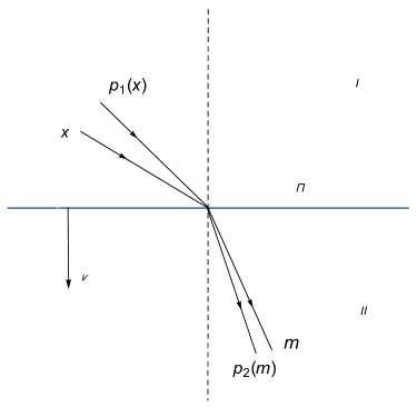
Figure 1. Snell’s law

We formulate the Snell law in anisotropic media as follows: Each incident ray traveling in medium $I$ with direction $x\in\Sigma_{1}$ with $x\cdot\nu\geq 0$ and striking the plane $\Pi$ at some point $P_{0}$ is refracted in medium $II$ into a direction $m\in\Sigma_{2}$ if

(3.1) $$p_{2}(m)-p_{1}(x)\parallel\nu,$$

with $p_{i}=\nabla N_{i}$, $i=1,2$; see Figure 1. For each $x\in\Sigma_{1}$ with $x\cdot\nu\geq 0$, there is at most one $m\in\Sigma_{2}$ satisfying (3.1) with $m\cdot\nu\geq 0$. In fact, from (3.1) there is $\lambda\in{\mathbb{R}}$ with $p_{2}(m)=p_{1}(x)+\lambda\,\nu$. That is, if $\ell$ is the line passing through $p_{1}(x)$ with direction $\nu$, then $p_{2}(m)\in\ell\cap\Sigma_{2}^{*}$. So if there were $m_{1}\neq m_{2}$ satisfying (3.1), then $p_{2}(m_{i})\in\ell\cap\Sigma_{2}^{*}$, $i=1,2$. The outer normal to $\Sigma_{2}^{*}$ at $p_{2}(m_{i})$ equals to $\nabla N_{2}^{*}\left(p_{2}(m_{i})\right)=p_{2}^{*}\left(p_{2}(m_{i})\right)=m_{i}$ because $p_{2}:\Sigma_{2}\to\Sigma_{2}^{*}$ is a homeomorphism since $\Sigma_{2}$ is $C^{1}$ and strictly convex. And also $p_{2}(m_{1})\neq p_{2}(m_{2})$. On the other hand, since the points $p_{2}(m_{i})$ are also on the line $\ell$ and $\Sigma_{2}^{*}$ is strictly convex, the normals at $p_{2}(m_{i})$ must satisfy that its dot products with $\nu$ must have different signs. Therefore, it cannot both happen $m_{1}\cdot\nu\geq 0$ and $m_{2}\cdot\nu\geq 0$. Therefore, only one of the two $m_{i}$ can satisfy $m_{i}\cdot\nu\geq 0$.

Physically, the norm $N(x)=1$ represents the location of the points $x$ after traveling for a time $t$, with $c\,t=1$, from the origin into the given medium. For example, if we are in an homogenous and isotropic medium with refractive index $n_{1}$, then the wave propagates from the origin with velocity $v_{1}=c/n_{1}$. So if $x$ satisfies $N(x)=1$, then the Euclidean distance from $O$ to $x$ must satisfy $|x|/t=v_{1}$. Since $t=1/c$, we obtain $|x|=v_{1}/c=1/n_{1}$ so $N(x)=n_{1}\,|x|$. Therefore, if medium $I$ has refractive index $n_{1}$ and medium $II$ has refractive index $n_{2}$, then $N_{1}(x)=n_{1}\,|x|$ and $N_{2}(x)=n_{2}\,|x|$. We then have $p_{i}(x)=\nabla N_{i}(x)=n_{i}\,\dfrac{x}{|x|}$, $i=1,2$, $x\neq 0$, and so from (3.1) we recover the standard Snell law: the unit incident direction $x$ is refracted into the unit direction $m$ when $n_{1}\,x-n_{2}\,m\parallel\nu$, see [GH09, Formula (2.1)].

We shall prove that (3.1) is equivalent to Fermat’s principle of least time with respect to the norms $N_{1},N_{2}$ where $\Sigma_{1}$ and $\Sigma_{2}$ strictly convex. Suppose two anisotropic media $I,II$ with norms $N_{1}$ in $I$ and $N_{2}$ in $II$, are separated by a plane $\Pi$ as in Figure 1. Given $X\in I$ and $Y\in II$, then Fermat’s principle states that the (minimal) optical path from $X$ to $Y$ through the plane $\Pi$ is the path $XP_{0}Y$ where $P_{0}\in\Pi$ is the unique point such that

(3.2) $$\min\{N_{1}(P-X)+N_{2}(Y-P):P\in\Pi\}=N_{1}(P_{0}-X)+N_{2}(Y-P_{0}).$$

Equation (3.2) implies that

(3.3) $$p_{2}(Y-P_{0})-p_{1}(P_{0}-X)\parallel\nu$$

where $\nu$ is the normal to $\Pi$. In fact, for $P\in\Pi$ we can write $P=P_{0}+\sum_{i=1}^{n-1}t_{i}\,e_{i}$ where $e_{1},\cdots,e_{n-1}$ is a basis for $\Pi$. From (3.2)

$$\dfrac{\partial}{\partial t_{j}}\left(N_{1}\left(P_{0}-X+\sum_{i=1}^{n-1}t_{i}\,e_{i}\right)+N_{2}\left(P_{0}-Y+\sum_{i=1}^{n-1}t_{i}\,e_{i}\right)\right)$$

$$=p_{1}\left(P_{0}-X+\sum_{i=1}^{n-1}t_{i}\,e_{i}\right)\cdot e_{j}+p_{2}\left(P_{0}-Y+\sum_{i=1}^{n-1}t_{i}\,e_{i}\right)\cdot e_{j}=0$$

when $t_{j}=0$, for $j=1,\cdots,n-1$. Since $p_{i}(-X)=-p_{i}(X)$, (3.3) follows. Also since $p_{i}$ are homogenous of degree zero, from (3.3) we then obtain (3.1) with $m=\dfrac{Y-P_{0}}{N_{2}(Y-P_{0})}$ and $x=\dfrac{P_{0}-X}{N_{1}(P_{0}-X)}$.

Vice versa, from (3.1) we deduce (3.2). In fact, let us fix $X\in I$ and $Y\in II$, and consider a path $XP_{0}Y$ with $P_{0}\in\Pi$. The ray from $X$ to $P_{0}$ has direction $x=\dfrac{P_{0}-X}{N_{1}(P_{0}-x)}$, and the ray from $P_{0}$ to $Y$ has direction $m=\dfrac{Y-P_{0}}{N_{2}(Y-P_{0})}$. If $x$ is refracted into $m$, then from (3.1), $p_{2}\left(\dfrac{Y-P_{0}}{N_{2}(Y-P_{0})}\right)-p_{1}\left(\dfrac{P_{0}-X}{N_{1}(P_{0}-x)}\right)\parallel\nu$, and since $p_{i}$ are homogeneous of degree zero

(3.4) $$p_{2}\left(Y-P_{0}\right)-p_{1}\left(P_{0}-X\right)\parallel\nu.$$

Consider the functional $F(P)=N_{1}(P-X)+N_{2}(Y-P)$ for $P\in\Pi$. Write $P\in\Pi$ as $P=P_{0}+\sum_{i=1}^{n-1}t_{i}\,e_{i}$ where $e_{1},\cdots,e_{n-1}$ is a basis for $\Pi$. We can write $F(P)=F(t_{1},\cdots,t_{n-1})$. As before and from (3.4)

$$\dfrac{\partial}{\partial t_{j}}F(t_{1},\cdots,t_{n-1})=p_{1}\left(P_{0}-X+\sum_{i=1}^{n-1}t_{i}\,e_{i}\right)\cdot e_{j}+p_{2}\left(P_{0}-Y+\sum_{i=1}^{n-1}t_{i}\,e_{i}\right)\cdot e_{j}=0$$

for $j=1,\cdots,n-1$ and $t_{1}=\cdots=t_{n-1}=0$. On the other hand, since the functional $F$ on $\Pi$ is strictly convex, there are unique $t_{1}^{0},\cdots,t_{n-1}^{0}$ such that the minimum of $F$ is attained at $t_{1}^{0},\cdots,t_{n-1}^{0}$. Therefore, $t_{1}^{0}=\cdots=t_{n-1}^{0}=0$ and the point $P_{0}$ is the unique point in $\Pi$ minimizing $F$, obtaining Fermat’s principle.

3.1. Physical constraints for refraction

Since the incident ray $x$ is in media $I$ we must have $x\cdot\nu\geq 0$, where $\nu$ is the normal to the hyperplane separating $I$ and $II$, $\nu$ having direction from media $I$ to media $II$. Similarly, since the refracted ray $m$ is in media $II$, we also have $m\cdot\nu\geq 0$; Figure 1.

We analyze here the meaning of these two physical constraints $x\cdot\nu\geq 0$ and $m\cdot\nu\geq 0$ in the following two cases.

Case 1: Let us assume first that $\Sigma_{1}$ is contained inside $\Sigma_{2}$, i.e., $N_{2}(x)\leq 1$ for all $N_{1}(x)=1$. If $x\in\Sigma_{1}$, then $p_{1}(x)\in\Sigma_{1}^{*}$ and from Lemma 2.1(b) $x\cdot p_{1}(x)=1$. Hence, if $x\in\Sigma_{1}$ and $m\in\Sigma_{2}$, then

$$x\cdot\left(p_{1}(x)-p_{2}(m)\right) =1-x\cdot p_{2}(m)$$

$$=1-N_{2}(x)\,\dfrac{x}{N_{2}(x)}\cdot p_{2}(m)\geq 1-N_{2}(x)\qquad\text{from Lemma \ref{lm:lemma 2.3 CH}(a)}$$

$$\geq 0\qquad\text{from the assumption $\Sigma_{1}$ contained inside $\Sigma_{2}$}.$$

Thus, if $x\cdot\nu\geq 0$ and $x$ is refracted into $m$, then from (3.1) $p_{1}(x)-p_{2}(m)=\lambda\,\nu$ and so $\lambda>0$. Hence, $m\cdot\nu\geq 0$ and Lemma 2.1(b) imply that

$$m\cdot p_{1}(x)-1=m\cdot\left(p_{1}(x)-p_{2}(m)\right)=\lambda\,m\cdot\nu\geq 0.$$

Therefore, when $\Sigma_{1}$ is contained in the interior of $\Sigma_{2}$, we obtain the physical constraint

(3.5) $$m\cdot p_{1}(x)\geq 1,$$

for refraction of $x\in\Sigma_{1}$ into $m\in\Sigma_{2}$.

Case 2: Let us assume now that $\Sigma_{2}$ is contained inside $\Sigma_{1}$, i.e., $N_{1}(x)\leq 1$ for all $N_{2}(x)=1$. Reasoning as in the first case, we have for $x\in\Sigma_{1}$ and $m\in\Sigma_{2}$, that

$$m\cdot\left(p_{2}(m)-p_{1}(x)\right) =1-m\cdot p_{1}(x)$$

$$=1-N_{1}(m)\,\dfrac{m}{N_{1}(m)}\cdot p_{1}(x)\geq 1-N_{1}(m)\qquad\text{from Lemma \ref{lm:lemma 2.3 CH}(a)}$$

$$\geq 0\qquad\text{from the assumption $\Sigma_{2}$ contained inside $\Sigma_{1}$}.$$

Thus, if $m\cdot\nu\geq 0$ and $x$ is refracted into $m$, then from (3.1) $p_{2}(m)-p_{1}(x)=\lambda\,\nu$ and so $\lambda>0$. Hence, $x\cdot\nu\geq 0$ and Lemma 2.1(b) imply that

$$x\cdot p_{2}(m)-1=x\cdot\left(p_{2}(m)-p_{1}(x)\right)=\lambda\,x\cdot\nu\geq 0.$$

Therefore, when $\Sigma_{2}$ is contained in the interior of $\Sigma_{1}$, we obtain the physical constraint

(3.6) $$x\cdot p_{2}(m)\geq 1,$$

for refraction of $x\in\Sigma_{1}$ into $m\in\Sigma_{2}$.

Notice that, as explained before, if medium $I$ has refractive index $n_{1}$ and medium $II$ has refractive index $n_{2}$, then $N_{1}(x)=n_{1}\,|x|$ and $N_{2}(x)=n_{2}\,|x|$; and $p_{i}(x)=n_{i}\,\dfrac{x}{|x|}$, $i=1,2$. Hence, if $n_{1}>n_{2}$ we are in Case 1 above, and so (3.5) reads $x\cdot m\geq n_{2}/n_{1}$ for $x,m$ unit vectors. If $n_{1}<n_{2}$ then we are then in Case 2, and so (3.6) reads $x\cdot m\geq n_{1}/n_{2}$ for $x,m$ unit vectors. Therefore, when the media $I$ and $II$ are homogenous and isotropic we recover the physical constraints showed in [GH09, Lemma 2.1].

4. Uniformly refracting surfaces

In this section, we shall describe the surfaces separating two anisotropic materials $I$ and $II$, like in Section 3, so that rays emanating from a point source, the origin, located in medium $I$ are refracted in medium $II$ into a fixed direction $m\in\Sigma_{2}$. These surfaces will have the form

(4.1) $$\left\{X\in{\mathbb{R}}^{n}:N_{1}(X)=p_{2}(m)\cdot X+b\right\},$$

where $b\in{\mathbb{R}}$. If we write $X=\rho(x)\,x$ for $N_{1}(x)=1$, then the polar radius

$$\rho(x)=\dfrac{b}{1-x\cdot p_{2}(m)}\qquad\text{for $x\in\Sigma_{1}$}.$$

To show that these surfaces do the desired refraction job, as in Section 3.1 we distinguish two cases.

Case I: $\Sigma_{1}$ is strictly contained in the interior of $\Sigma_{2}$, that is,

(4.2) $$\kappa=\sup_{N_{1}(x)=1}N_{2}(x)<1.$$

In this case, given $m\in\Sigma_{2}$, the desired surface is

(4.3) $$S_{I}(m,b)=\left\{\rho(x)x:\rho(x)=\dfrac{b}{1-x\cdot p_{2}(m)},\text{ $x\in\Sigma_{1}$ with $m\cdot p_{1}(x)\geq 1$}\right\}$$

with $b>0$. In fact, to verify that each ray with direction $x\in\Sigma_{1}$ such that $m\cdot p_{1}(x)\geq 1$ is refracted by $S_{I}(m,b)$ into $m$, we need to verify that (3.1) holds, and the physical constraints $x\cdot\nu\geq 0$ and $m\cdot\nu\geq 0$ are met with $\nu$ the normal from medium $I$ to $II$. From (4.1), the outward normal at a point $X$ is $\nu=p_{1}(x)-p_{2}(m)$ with $x=X/N_{1}(X)$ and so (3.1) holds. From Lemma 2.1

$$x\cdot\nu =x\cdot\left(p_{1}(x)-p_{2}(m)\right)=1-x\cdot p_{2}(m)$$

(4.4) $$=1-N_{2}(x)\,\dfrac{x}{N_{2}(x)}\cdot p_{2}(m)\geq 1-N_{2}(x)>1-\kappa>0$$

from (4.2). Also $m\cdot\nu=m\cdot\left(p_{1}(x)-p_{2}(m)\right)=m\cdot p_{1}(x)-m\cdot p_{2}(m)=m\cdot p_{1}(x)-1\geq 0$ by the definition of $S_{I}$.

Case II: $\Sigma_{2}$ is strictly contained in the interior of $\Sigma_{1}$, that is,

(4.5) $$\kappa=\inf_{N_{1}(x)=1}N_{2}(x)>1.$$

In this case, given $m\in\Sigma_{2}$, the desired surface is

(4.6) $$S_{II}(m,b)=\left\{\rho(x)x:\rho(x)=\dfrac{b}{x\cdot p_{2}(m)-1},\text{ $x\in\Sigma_{1}$ with $x\cdot p_{2}(m)>1$}\right\}$$

with $b>0$. In fact and once again, to verify that each ray with direction $x\in\Sigma_{1}$ such that $x\cdot p_{2}(m)>1$ is refracted by $S_{II}(m,b)$ into $m$, we need to verify that (3.1) holds, and the physical constraints $x\cdot\nu\geq 0$ and $m\cdot\nu\geq 0$ are met with $\nu$ the normal towards medium $II$. From the definition of $S_{II}$, the outward normal at a point $X$ is $\nu=p_{2}(m)-p_{1}(x)$ with $x=X/N_{1}(X)$ and so (3.1) holds. From Lemma 2.1

$$m\cdot\nu =m\cdot\left(p_{2}(m)-p_{1}(x)\right)=1-m\cdot p_{1}(x)$$

$$=1-N_{1}(m)\,\dfrac{m}{N_{1}(m)}\cdot p_{1}(x)\geq 1-N_{1}(m)\geq 1-\dfrac{1}{\kappa}\,N_{2}(m)=1-\dfrac{1}{\kappa}>0$$

from (4.5). Also $x\cdot\nu=x\cdot\left(p_{2}(m)-p_{1}(x)\right)=x\cdot p_{2}(m)-1>0$ by the definition of $S_{II}$.

Remark 4.1.

If medium $I$ is homogeneous and isotropic with refractive index $n_{1}$, then $N_{1}(x)=n_{1}\,|x|$. Also, if $II$ is also similar with refractive index $n_{2}$, then $N_{2}(x)=n_{2}\,|x|$. In this case, condition (4.2) is equivalent to $n_{1}>n_{2}$, and the surface $S_{I}(m,b)$ is a half ellipsoid of revolution with axis $m$, recovering the surfaces from [GH09, Formula (2.8)]. Similarly, condition (4.5) is equivalent to $n_{1}<n_{2}$, and $S_{II}(m,b)$ is one of the branches of a hyperboloid of two sheets as in [GH09, Formula (2.9)].

5. The refractor problem when $\kappa<1$, $\kappa$ in (4.2)

Using the uniformly refracting surfaces introduced in Section 4, we state and solve here the refraction problem we are interested in.

We are given two closed domains $\Omega_{1}\subset\Sigma_{1}$, $\Omega_{2}\subset\Sigma_{2}$, a non negative function $f\in L^{1}(\Omega_{1})$, and a Radon measure $\mu$ in $\Omega_{2}$ satisfying the following conditions:

1. the surface measure of the boundary of $\Omega_{1}$ is zero;

2. $\inf_{x\in\Omega_{1},m\in\Omega_{2}}m\cdot p_{1}(x)\geq 1$;

3. $\Sigma_{1}$ and $\Sigma_{2}$ are $C^{1}$ and strictly convex.

Refractors are then defined as follows.

Definition 5.1.

The surface $S=\{\rho(x)\,x:x\in\Omega_{1}\}$, with $\rho\in C(\Omega_{1})$, $\rho>0$, is a refractor from $\Omega_{1}$ to $\Omega_{2}$, if for each $x_{0}\in\Omega_{1}$ there exist $m\in\Omega_{2}$ and $b>0$ such that the surface $S_{I}(m,b)$ supports $S$ at $x_{0}$, that is,

$$\rho(x)\leq\dfrac{b}{1-x\cdot p_{2}(m)}\quad\text{for all $x\in\Omega_{1}$ with equality at $x=x_{0}$}.$$

The refractor mapping associated with the refractor $S$ is the set valued function

(5.1) $$\mathcal{R}_{S}(x_{0})=\{m\in\Omega_{2}:\text{there exists $S_{I}(m,b)$ supporting $S$ at $x_{0}$}\}.$$

We have the following lemma.

Lemma 5.2.

If a refractor $S$ is parametrized by $\rho(x)\,x$, then $\rho$ is Lipschitz continuous in $\Omega_{1}$.

Proof.

Let $x_{0},x\in\Omega_{1}$ and $S_{I}(m,b)$ supporting $S$ at $x_{0}$. Then

$$\rho(x)-\rho(x_{0}) \leq\dfrac{b}{1-x\cdot p_{2}(m)}-\dfrac{b}{1-x_{0}\cdot p_{2}(m)}=b\,\dfrac{(x-x_{0})\cdot p_{2}(m)}{\left(1-x\cdot p_{2}(m)\right)\left(1-x_{0}\cdot p_{2}(m)\right)}$$

$$=\rho(x_{0})\,\dfrac{(x-x_{0})\cdot p_{2}(m)}{1-x\cdot p_{2}(m)}\leq\max_{\Omega_{1}}\rho\,\dfrac{|x-x_{0}|\,|p_{2}(m)|}{1-\kappa}\qquad\text{from \eqref{eq:1-x p2m>1-kappa}}$$

$$\leq C\,|x-x_{0}|$$

since $N_{i}$ and $|\cdot|$ are all equivalent norms, $i=1,2$. Reversing the roles of $x$ and $x_{0}$ we obtain the lemma. ∎

Following the notation from [GH14, Section 2], we denote by $C_{S}(\Omega_{1},\Omega_{2})$ the class of set-valued maps $\Phi:\Omega_{1}\to\Omega_{2}$ that are single valued for a.e. $x\in\Omega_{1}$, with respect to $f\,dx$, that are continuous in $\Omega_{1}$, and $\Phi(\Omega_{1})=\Omega_{2}$. Continuity of $\Phi$ at $x_{0}\in\Omega_{1}$ means that if $x_{k}\to x_{0}$ and $y_{k}\in\Phi(x_{k})$, then there is a subsequence $y_{k_{j}}$ and $y_{0}\in\Phi(x_{0})$ such that $y_{k_{j}}\to y_{0}$.

Lemma 5.3.

If $S$ is a refractor from $\Omega_{1}$ to $\Omega_{2}$, then the refractor map $\mathcal{R}_{S}\in C_{S}(\Omega_{1},\Omega_{2})$.

Proof.

Let $m\in\Omega_{2}$ and define $b=\max_{x\in\Omega_{1}}\left(\rho(x)\,(1-x\cdot p_{2}(m)\right)$. From (4), $b\geq\max_{x\in\Omega_{1}}\left(\rho(x)\,(1-\kappa)\right)>0$. Also, there is $x_{0}\in\Omega_{1}$ with $b=\rho(x_{0})\,\left(1-x_{0}\cdot p_{2}(m)\right)$ and so $m\in\mathcal{R}_{S}(x_{0})$, showing that $\mathcal{R}_{S}(\Omega_{1})=\Omega_{2}$.

Next, let us show that $\mathcal{R}_{S}(x)$ is single valued for a.e. $x\in\Omega_{1}$. In fact, if at $x_{0}\in\Omega_{1}$ there exist $m_{1}\neq m_{2}\in\Omega_{2}$ with $m_{i}\in\mathcal{R}_{S}(x_{0})$, $i=1,2$, then $x_{0}$ is a singular point to the surface $S$. Otherwise, since $S_{I}(m_{i},b_{i})$, $i=1,2$ support $S$ at $x_{0}$, they would have the same tangent plane at $x_{0}\rho(x_{0})$. Therefore, by the Snell law and since there is at most one $m$ satisfying (3.1), we obtain $m_{1}=m_{2}$. From Lemma 5.2, $S$ is Lipschitz, and since $|\partial\Omega_{1}|=0$, we obtain that $\mathcal{R}_{S}(x)$ is single valued a.e. in $\Omega_{1}$.

It remains to show that $\mathcal{R}_{S}$ is continuous. Let $x_{i}\to x_{0}\in\Omega_{1}$ and let $m_{i}\in\mathcal{R}_{S}(x_{i})$. Hence $\rho(x)\leq\dfrac{b_{i}}{1-x\cdot p_{2}(m_{i})}$ for all $x\in\Omega_{1}$ with equality at $x=x_{i}$. As before, $b_{i}=\rho(x_{i})\,\left(1-x_{i}\cdot p_{2}(m_{i})\right)\geq(1-\kappa)\,\min_{\Omega_{1}}\rho$, and $b_{i}=\rho(x_{i})\left(1-N_{2}(x_{i})\,\dfrac{x_{i}}{N_{2}(x_{i})}\cdot p_{2}(m_{i})\right)\leq\max_{\Omega_{1}}\rho\,(1+\kappa)$ from Lemma 2.1(a) and (4.2). We have $m_{i}\in\Omega_{2}\subset\Sigma_{2}$ and $p_{2}\in C\left(\Sigma_{2}\right)$. By compactness there are subsequences $m_{i_{k}}\to m_{0}\in\Omega_{2}$ and $b_{i_{k}}\to b_{0}>0$ so that $\rho(x)\leq\dfrac{b_{0}}{1-x\cdot p_{2}(m_{0})}$ for all $x\in\Omega_{1}$ with equality at $x=x_{0}$. This completes the proof to the lemma.

∎

Using [GH14, Lemma 2.1], we obtain from Lemma 5.3 that if $S$ is a refractor from $\Omega_{1}$ to $\Omega_{2}$, then the set function

(5.2) $$\mathcal{M}_{S,f}(E)=\int_{\mathcal{R}_{S}^{-1}(E)}f(x)\,dx$$

is a Borel measure in $\Omega_{2}$, that is called the refractor measure.

Continuing using the set up from [GH14, Section 2], we recall [GH14, Definition 2.2]: given $\mathcal{F}\subset C(\Omega_{1})$ and a map $\mathcal{T}:\mathcal{F}\to C_{S}(\Omega_{1},\Omega_{2})$, we say $\mathcal{T}$ is continuous at $\phi\in\mathcal{F}$ if whenever $\phi_{j}\in\mathcal{F}$, $\phi_{j}\to\phi$ uniformly in $\Omega_{1}$, $x_{0}\in\Omega_{1}$ and $y_{j}\in\mathcal{T}(\phi_{j})(x_{0})$, then there exists a subsequence $y_{j_{\ell}}\to y_{0}$ with $y_{0}\in\mathcal{T}(\phi)(x_{0})$. If we let

(5.3) $$\mathcal{F}=\{\rho\in C(\Omega_{1}):S_{\rho}\text{ is a refractor from $\Omega_{1}$ to $\Omega_{2}$ parametrized by $\rho(x)x$}\}$$

then we have the following lemma.

Lemma 5.4.

The mapping $\mathcal{T}:\mathcal{F}\to C_{S}(\Omega_{1},\Omega_{2})$ defined by $\mathcal{T}(\rho)=\mathcal{R}_{S_{\rho}}$ is continuous at each $\rho\in\mathcal{F}$.

Proof.

Let $\rho_{j},\rho\in\mathcal{F}$ with $\rho_{j}\to\rho$ uniformly in $\Omega_{1}$, $x_{0}\in\Omega_{1}$ and $m_{j}\in\mathcal{R}_{S_{\rho_{j}}}(x_{0})$. Hence $\rho_{j}(x)\leq\dfrac{b_{j}}{1-x\cdot p_{2}(m_{j})}$ for all $x\in\Omega_{1}$ with equality at $x=x_{0}$. As in the last part of the proof of Lemma 5.3, $b_{j}$ are bounded away from $0$ and $\infty$. Therefore there exist subsequences $b_{j_{\ell}}\to b$ and $m_{j_{\ell}}\to m$ with $\rho(x)\leq\dfrac{b}{1-x\cdot p_{2}(m)}$ for all $x\in\Omega_{1}$ with equality at $x=x_{0}$. Thus $m\in\mathcal{R}_{S_{\rho}}(x_{0})$ and we are done. ∎

As a consequence of Lemma 5.4 we obtain from [GH14, Lemma 2.3] that

if $$\rho_{j}\to\rho \Omega_{1} \mathcal{M}_{S_{\rho_{j}},f}\to\mathcal{M}_{S_{\rho},f}$$ uniformly in , then weakly.

In addition, properties (A1)-(A3) from [GH14, Section 2.1] translate to the present case as follows:

1. if $S_{\rho_{1}}$ and $S_{\rho_{2}}$ are refractors from $\Omega_{1}$ to $\Omega_{2}$, then $S_{\rho_{1}\wedge\rho_{2}}$ is a refractor from $\Omega_{1}$ to $\Omega_{2}$ with $\rho_{1}\wedge\rho_{2}=\min\{\rho_{1},\rho_{2}\}$;

2. if $\rho_{1}(x_{0})\leq\rho_{2}(x_{0})$, then $\mathcal{R}_{S_{\rho_{1}}}(x_{0})\subset\mathcal{R}_{S_{\rho_{1}\wedge\rho_{2}}}(x_{0})$;

3. we let $h_{b,m}(x)=\dfrac{b}{1-x\cdot p_{2}(m)}$, and we have

   $$\{h_{b,m}(x):m\in\Omega_{2},0<b<\infty\}\subset\mathcal{F},$$

   with $\mathcal{F}$ defined by (5.3). In addition we have the following

   1. $m\in\mathcal{R}_{S_{h_{b,m}}}(x)$ for all $x\in\Omega_{1}$, from Section 4, Case I;

   2. $h_{b_{1},m}\leq h_{b_{2},m}$ for $b_{1}\leq b_{2}$;

   3. $h_{b,m}\to 0$ uniformly in $\Omega_{1}$ as $b\to 0$;

   4. $h_{b,m}\to h_{b_{0},m}$ uniformly in $\Omega_{1}$ as $b\to b_{0}$.

We then introduce the following definition.

Definition 5.5.

Let $f\in L^{1}(\Omega_{1})$ and let $\mu$ be a Radon measure in $\Omega_{2}$ with $\int_{\Omega_{1}}f\,dx=\mu(\Omega_{2})$. The refractor $S$ from $\Omega_{1}$ to $\Omega_{2}$ is a weak solution of the refractor problem if

$$\mathcal{M}_{S,f}(E)=\mu(E)$$

for each Borel set $E\subset\Omega_{2}$, where $\mathcal{M}_{S,f}$ is the refractor measure defined by (5.2).

Using the above set up and the existence results from [GH14, Section 2] we obtain the following theorems showing solvability of the refractor problem for anisotropic media when $\kappa<1$. We first show solvability when the measure $\mu$ is discrete.

Theorem 5.6.

Let $f\in L^{1}(\Omega_{1})$ with $f>0$ a.e., $m_{1},\cdots,m_{N}\in\Omega_{2}$ be distinct points, and $g_{1},\cdots,g_{N}$ positive numbers satisfying $\int_{\Omega_{1}}f\,dx=\sum_{i=1}^{N}g_{i}$.

Then for each $0<b_{1}<\infty$ there exist unique positive $b_{2},\cdots,b_{N}$ such that

$$S=\{\rho(x)x:x\in\Omega_{1}\}\text{ with }\rho(x)=\min_{1\leq i\leq N}h_{b_{i},m_{i}}(x),$$

is a weak solution to the refractor problem. In addition, $\mathcal{M}_{S,f}(\{m_{i}\})=g_{i}$ for $1\leq i\leq N$.

Proof.

To prove this theorem, we use [GH14, Theorem 2.5] with the set up from above, for which we need to verify that the assumptions of that theorem are met. In fact, we need to show that we can choose positive numbers $b_{2}^{0},\cdots,b_{N}^{0}$ such that $\rho_{0}(x)=\min_{1\leq i\leq N}h_{b_{i}^{0},m_{i}}(x)$ such that $\mathcal{M}_{S_{\rho_{0}},f}(m_{i})\leq g_{i}$ for $2\leq i\leq N$, where $b_{1}^{0}=b_{1}$. We have $h_{b_{1}^{0},m_{1}}(x)=\dfrac{b_{1}^{0}}{1-x\cdot p_{2}(m_{1})}\leq\dfrac{b_{1}}{1-\kappa}$ from (4). Also $h_{b_{i}^{0},m_{i}}(x)=\dfrac{b_{i}^{0}}{1-x\cdot p_{2}(m_{i})}\geq\dfrac{b_{i}^{0}}{1+\kappa}$ for $2\leq i\leq N$ from Lemma 2.1(b) and (4.2). Therefore choosing $b_{2}^{0},\cdots,b_{N}^{0}$ suitable so that $\rho_{0}(x)=h_{b_{1}^{0},m_{1}}(x)$, the assumptions of [GH14, Theorem 2.5] are met and the existence follows. The uniqueness follows from [GH14, Theorem 2.7] since $f>0$ a.e. ∎

We are now ready to prove the following existence theorem for a general Radon measure $\mu$.

Theorem 5.7.

Let $f\in L^{1}(\Omega_{1})$ with $f>0$ a.e, and let $\mu$ be a Radon measure in $\Omega_{2}$ such that $\int_{\Omega_{1}}f(x)\,dx=\mu\left(\Omega_{2}\right)$. Then for each $x_{0}\in\Omega_{1}$ and $R_{0}>0$, there exists $\mathcal{S}$ weak solution to the refractor problem passing through the point $X_{0}=R_{0}\,x_{0}$.

Proof.

Let $\mu_{\ell}=\sum_{i=1}^{N}g_{i}\,\delta_{m_{i}}$ be a sequence of discrete measures with $\mu_{\ell}\to\mu$ weakly and $\mu_{\ell}\left(\Omega_{2}\right)=\mu\left(\Omega_{2}\right)$ for $\ell=1,2,\cdots$. From Theorem 5.6 and for the measure $\mu_{\ell}$, there exists a refractor $S_{\rho_{\ell}^{*}}$ parametrized by $\rho_{\ell}^{*}$. Notice that $S_{C_{\ell}\,\rho_{\ell}^{*}}$ is also a solution to the same refractor problem since $\mathcal{R}_{C_{\ell}\,\rho_{\ell}^{*}}=\mathcal{R}_{\rho_{\ell}^{*}}$ for each positive constant $C_{\ell}$. Then pick $C_{\ell}$ so that $C_{\ell}\,\rho^{*}_{\ell}(x_{0})=R_{0}$. Now we use the existence result [GH14, Theorem 2.8], and in order to do that we need to verify that the hypotheses (i) and (ii) of that theorem hold in the present case. To verify (i) we show that if $R_{1}\in\text{Range}\left(h_{b,m}\right)$, then

$$R_{1}\,\dfrac{1-\kappa}{1+\kappa}\leq h_{b,m}\leq R_{1}\,\dfrac{1+\kappa}{1-\kappa}.$$

In fact, there exists $x_{1}\in\Omega_{1}$ with $R_{1}=h_{b,m}(x_{1})=\dfrac{b}{1-x_{1}\cdot p_{2}(m)}$, so $h_{b,m}(x)=\dfrac{b}{1-x\cdot p_{2}(m)}=R_{1}\,\dfrac{1-x_{1}\cdot p_{2}(m)}{1-x\cdot p_{2}(m)}$, and the desired inequalities follow from Lemma 2.1(b) and (4.2). The verification of (ii), that is, the family $\{\rho\in\mathcal{F}:C_{0}\leq\rho\leq C_{1}\}$ is compact in $C(\Omega_{1})$, follows from Lemma 5.2 and the proof of Lemma 5.4. ∎

Remark 5.8.

In the same way we can state and solve the refractor problem when $\kappa>1$, i.e., (4.5) holds, using instead the uniformly refracting surfaces $S_{II}(m,b)$ defined by (4.6). Now the functions $h_{b,m}$ are defined by $h_{b,m}(x)=\dfrac{b}{x\cdot p_{2}(m)-1}$ and the properties (A1)-(A3) defined after Lemma 5.4 must be changed in accordance with properties (A1’)-(A3’) in [GH14, Section 2.2]. All lemmas in this section then hold true with obvious changes. For the existence of solutions we now need to use [GH14, Theorems 2.9 and 2.11].

In Theorem 5.7 uniqueness follows from optimal mass transport, Section 7.

6. Propagation of light in anisotropic materials

We begin this section with some background on the propagation of light in anisotropic materials. Let us assume we have a material whose permittivity and permeability are given by positive definite and symmetric matrices $\epsilon(x,y,z)$ and $\mu(x,y,z)$, respectively. Assuming we are in the geometric optics regime, i.e., the wave length of the radiation is very small compared with the objects considered, it is known [KK65, Chap. III, Sect. 4] that the function $\psi=\psi(x,y,z)$ defining the wave fronts $\psi(x,y,z)$=constant, satisfies the following first order pde, the Fresnel differential equation:

(6.1) $$\det\left(\begin{matrix}\epsilon&R\\ -R&\mu\end{matrix}\right)=0,$$

where $R$ is the $3\times 3$ skew-symmetric matrix

$$R=\left(\begin{matrix}0&-\psi_{z}&\psi_{y}\\ \psi_{z}&0&-\psi_{x}\\ -\psi_{y}&\psi_{x}&0\end{matrix}\right).$$

We can re write Fresnel’s equation in a simpler form using the following Schur’s determinant identity: if $A$ is an $n\times n$ invertible matrix, $B$ is $n\times m$, $C$ is $m\times n$ and $D$ is $m\times m$, then

$$\det\left(\begin{matrix}A&B\\ C&D\end{matrix}\right)=\det A\,\det\left(D-C\,A^{-1}\,B\right)=\det D\,\det\left(A-B\,D^{-1}\,C\right),$$

of course for the last identity $D$ is invertible. We then get

$$\det\left(\begin{matrix}\epsilon&R\\ -R&\mu\end{matrix}\right)=\det\epsilon\,\det\left(\mu+R\,\epsilon^{-1}\,R\right)=\det\mu\,\det\left(\epsilon+R\,\mu^{-1}\,R\right)$$

and since $\epsilon,\mu$ are positive definite, (6.1) is equivalent to either

(6.2) $$\det\left(\mu+R\,\epsilon^{-1}\,R\right)=0,$$

or

(6.3) $$\det\left(\epsilon+R\,\mu^{-1}\,R\right)=0.$$

Letting

(6.4) $$\tau=\mu^{-1/2}\epsilon\mu^{-1/2},$$

$\tau$ is symmetric and positive definite, so there is an orthogonal matrix $O$ and a diagonal matrix $D$ such that

$$\tau=ODO^{t}.$$

For a column vector $v=\left(\begin{matrix}v_{1}\\ v_{2}\\ v_{3}\end{matrix}\right)$ define

$$\text{Skew}(v)=\left(\begin{matrix}0&-v_{3}&v_{2}\\ v_{3}&0&-v_{1}\\ -v_{2}&v_{1}&0\end{matrix}\right).$$

Given a $3\times 3$ matrix $B$ we have the formula

$$B^{t}\,\text{Skew}(B\,v)\,B =\det B\,\text{Skew}(v).$$

We then re write (6.3) as follows:

$$\det\left(\epsilon+R\,\mu^{-1}\,R\right) =\det\mu\,\det\left(\mu^{-1/2}\epsilon\mu^{-1/2}+\left(\mu^{-1/2}R\mu^{-1/2}\right)\left(\mu^{-1/2}R\mu^{-1/2}\right)\right).$$

Also since $\mu^{-1/2}$ is symmetric, we have

$$\mu^{-1/2}R\mu^{-1/2}=\mu^{-1/2}\text{Skew}(\nabla\psi)\mu^{-1/2} =\mu^{-1/2}\text{Skew}\left(\mu^{-1/2}\mu^{1/2}\nabla\psi\right)\mu^{-1/2}$$

$$=\det\left(\mu^{-1/2}\right)\,\text{Skew}\left(\mu^{1/2}\nabla\psi\right).$$

Also

$$\mu^{-1/2}\epsilon\mu^{-1/2}+\left(\mu^{-1/2}R\mu^{-1/2}\right)\left(\mu^{-1/2}R\mu^{-1/2}\right)$$

$$=ODO^{t}+OO^{t}\left(\mu^{-1/2}R\mu^{-1/2}\right)OO^{t}\left(\mu^{-1/2}R\mu^{-1/2}\right)OO^{t}$$

$$=O\left(D+O^{t}\left(\mu^{-1/2}R\mu^{-1/2}\right)OO^{t}\left(\mu^{-1/2}R\mu^{-1/2}\right)O\right)O^{t}.$$

We have

$$\bar{R}:=O^{t}\left(\mu^{-1/2}R\mu^{-1/2}\right)O =\det\left(\mu^{-1/2}\right)O^{t}\,\text{Skew}\left(\mu^{1/2}\nabla\psi\right)\,O$$

$$=\det\left(\mu^{-1/2}\right)O^{t}\,\text{Skew}\left(O\,O^{t}\mu^{1/2}\nabla\psi\right)\,O$$

$$=\det\left(\mu^{-1/2}\right)\,\det O\,\text{Skew}\left(O^{t}\mu^{1/2}\nabla\psi\right),$$

so

$$D+\bar{R}\bar{R} =D+\left(\det\left(\mu^{-1/2}\right)\right)^{2}\,\left(\det O\right)^{2}\,\text{Skew}\left(O^{t}\mu^{1/2}\nabla\psi\right)\,\text{Skew}\left(O^{t}\mu^{1/2}\nabla\psi\right)$$

$$=D+\left(\det\left(\mu^{-1/2}\right)\right)^{2}\,\text{Skew}\left(O^{t}\mu^{1/2}\nabla\psi\right)\,\text{Skew}\left(O^{t}\mu^{1/2}\nabla\psi\right)$$

$$=D+\text{Skew}\left(O^{t}\dfrac{\mu^{1/2}}{\det\left(\mu^{1/2}\right)}\nabla\psi\right)\,\text{Skew}\left(O^{t}\dfrac{\mu^{1/2}}{\det\left(\mu^{1/2}\right)}\nabla\psi\right).$$

Therefore

$$\det\left(\epsilon+R\,\mu^{-1}\,R\right) =\det\mu\,\det\left(D+\text{Skew}\left(O^{t}\dfrac{\mu^{1/2}}{\det\left(\mu^{1/2}\right)}\nabla S\right)\,\text{Skew}\left(O^{t}\dfrac{\mu^{1/2}}{\det\left(\mu^{1/2}\right)}\nabla S\right)\right)$$

(6.5) $$=\det\mu\,\det\left(D+\text{Skew}(p)\,\text{Skew}(p)\right)=0,$$

where

$$p=\left(\begin{matrix}p_{1}\\ p_{2}\\ p_{3}\end{matrix}\right):=O^{t}\dfrac{\mu^{1/2}}{\det\left(\mu^{1/2}\right)}\nabla S.$$

Notice that this calculation is done at a fixed point $(x,y,z)$ since the matrices $\epsilon$ and $\mu$ depend on the point $(x,y,z)$; therefore the matrices $D$ and $O$ depend also on $(x,y,z)$. Next we have

$$\text{Skew}(p)\,\text{Skew}(p)=p\,p^{t}-p^{t}\,p\,Id=p\otimes p-(p\cdot p)\,Id,$$

so by (6) the Fresnel equation for the wave fronts (6.3) is then

$$0=\det\left(D+\text{Skew}(p)\,\text{Skew}(p)\right)=\det\left(D+p\otimes p-(p\cdot p)\,Id\right).$$

To write this equation in a more convenient form, set

$$D=\left(\begin{matrix}\tau_{1}&0&0\\ 0&\tau_{2}&0\\ 0&0&\tau_{3}\end{matrix}\right),$$

(a matrix depending on $(x,y,z)$), so

$$0 =\det\left(D+p\otimes p-(p\cdot p)\,Id\right)$$

$$=\det\left(\begin{matrix}\tau_{1}+p_{1}^{2}-|p|^{2}&p_{1}p_{2}&p_{1}p_{3}\\ p_{2}p_{1}&\tau_{2}+p_{2}^{2}-|p|^{2}&p_{2}p_{3}\\ p_{3}p_{1}&p_{3}p_{2}&\tau_{3}+p_{3}^{2}-|p|^{2}\\ \end{matrix}\right)$$

$$=\det\left(\begin{matrix}\tau_{1}-p_{2}^{2}-p_{3}^{2}&p_{1}p_{2}&p_{1}p_{3}\\ p_{2}p_{1}&\tau_{2}-p_{1}^{2}-p_{3}^{2}&p_{2}p_{3}\\ p_{3}p_{1}&p_{3}p_{2}&\tau_{3}-p_{1}^{2}-p_{2}^{2}\\ \end{matrix}\right).$$

Let us now define for an arbitrary vector $(p_{1},p_{2},p_{3})$ the following functions, which depend on the point $(x,y,z)$ since $\tau_{i}$ depend on $(x,y,z)$

$$\Phi(p_{1},p_{2},p_{3})=\dfrac{1}{2}\left(\dfrac{1}{\tau_{2}}+\dfrac{1}{\tau_{3}}\right)p_{1}^{2}+\dfrac{1}{2}\left(\dfrac{1}{\tau_{1}}+\dfrac{1}{\tau_{3}}\right)p_{2}^{2}+\dfrac{1}{2}\left(\dfrac{1}{\tau_{1}}+\dfrac{1}{\tau_{2}}\right)p_{3}^{2},$$

and

$$\Psi(p_{1},p_{2},p_{3})=(p_{1}^{2}+p_{2}^{2}+p_{3}^{2})\left(\dfrac{1}{\tau_{2}\tau_{3}}p_{1}^{2}+\dfrac{1}{\tau_{1}\tau_{3}}p_{2}^{2}+\dfrac{1}{\tau_{1}\tau_{2}}p_{3}^{2}\right).$$

It is easy to check that

(6.6) $$\dfrac{1}{\tau_{1}\tau_{2}\tau_{3}}\det\left[\begin{matrix}\tau_{1}-p_{2}^{2}-p_{3}^{2}&p_{1}p_{2}&p_{1}p_{3}\\ p_{2}p_{1}&\tau_{2}-p_{1}^{2}-p_{3}^{2}&p_{2}p_{3}\\ p_{3}p_{1}&p_{3}p_{2}&\tau_{3}-p_{1}^{2}-p_{2}^{2}\\ \end{matrix}\right]=1-2\Phi(p_{1},p_{2},p_{3})+\Psi(p_{1},p_{2},p_{3}).$$

Now write

$$1-2\Phi+\Psi=1-2\Phi+\Phi^{2}-\Phi^{2}+\Psi=(1-\Phi)^{2}-(\Phi^{2}-\Psi).$$

Next notice that

(6.7) $$\Phi^{2}\geq\Psi,$$

which follows using Legrange multipliers since $\Phi^{2}-\Psi$ is homogenous of degree four. So we can write

$$1-2\Phi+\Psi=\left(1-\Phi-\sqrt{\Phi^{2}-\Psi}\right)\,\left(1-\Phi+\sqrt{\Phi^{2}-\Psi}\right).$$

We then obtain that the Fresnel equation of wave fronts (6.3) can be split as the following two equations

(6.8) $$1-\Phi-\sqrt{\Phi^{2}-\Psi}=0\qquad\text{or}\qquad 1-\Phi+\sqrt{\Phi^{2}-\Psi}=0.$$

Each of these equations describes a three dimensional surface that depends of the point $(x,y,z)$ chosen at the beginning; see Figure 2. That is, in this way each point $(x,y,z)$ in the space has associated a pair of surfaces, one enclosing the other. The inner surface is convex and the outer surface is neither convex nor concave. We have shown that the vector

(6.9) $$p=\left(\begin{matrix}p_{1}\\ p_{2}\\ p_{3}\end{matrix}\right):=O^{t}\dfrac{\mu^{1/2}}{\det\left(\mu^{1/2}\right)}\nabla\psi,$$

belongs to one of the surfaces, with all quantities calculated at $(x,y,z)$, and the matrix $O$ is orthogonal and diagonalizes the matrix $\tau$. In other words, we have shown that the gradient $\nabla\psi(x,y,z)$ of the wave front $\psi$=constant, when multiplied by the matrix $\dfrac{\mu^{1/2}}{\det\left(\mu^{1/2}\right)}$ and conveniently rotated by $O^{t}$, belongs to one of the surfaces described by the equations (6.8).

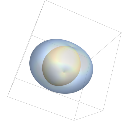
Figure 2. Fresnel surfaces when $\tau_{1}=1,\tau_{2}=2,\tau_{3}=3$; $\mu=Id$

Notice that when the permittivity matrix is $\epsilon\,Id$ and the permeability matrix is $\mu\,Id$, where $\epsilon$ and $\mu$ are scalar functions depending only on position, then we recover the eikonal equation $|\nabla\psi|^{2}=\epsilon\,\mu$. In fact, in this case the matrix $\tau=(\epsilon/\mu)\,Id$, so $\tau_{i}=\epsilon/\mu$ for $i=1,2,3$, $O=Id$,

$$\Phi(p_{1},p_{2},p_{3})=\dfrac{\mu}{\epsilon}(p_{1}^{2}+p_{2}^{2}+p_{3}^{2}),$$

and

$$\Psi(p_{1},p_{2},p_{3})=\left(\dfrac{\mu}{\epsilon}\right)^{2}(p_{1}^{2}+p_{2}^{2}+p_{3}^{2})^{2}.$$

So $\Phi^{2}=\Psi$ and both surfaces in (6.8) are identically equal to

$$1-\Phi(p_{1},p_{2},p_{3})=1-\dfrac{\mu}{\epsilon}(p_{1}^{2}+p_{2}^{2}+p_{3}^{2})=0.$$

So the vector $p$ in (6.9) satisfies the last equation and $p=\dfrac{1}{\mu}\nabla\psi$, therefore $|\nabla\psi|^{2}=\epsilon\,\mu$.

6.1. Case considered for the application of our results

For the application of our results from Sections 3–5 we consider materials having permittivity and permeability tensors $\epsilon$ and $\mu$ that are positive definite symmetric constant matrices with $\mu=a\,\epsilon$, where $a$ is a positive number. These are homogeneous materials that when $\epsilon$ is not the identity matrix are anisotropic. We will associate with such a material a norm as follows. From the calculations above, the Fresnel equation in this case is as follows. From (6.4) we get $\tau=\dfrac{1}{a}\,Id$, so

$$\Phi(p)=a\,|p|^{2},\qquad\Psi(p)=a^{2}\,|p|^{4}.$$

Obviously, $\Phi^{2}=\Psi$ and so the Fresnel equation is $1-\Phi=0$, i.e., $|p|^{2}=1/a$ and therefore it has only one sheet. Then from (6.9) the vector $\dfrac{\mu^{1/2}}{\det\mu^{1/2}}\,\nabla\psi$ satisfies the equation

$$\left|\dfrac{\sqrt{a}\,\mu^{1/2}}{\det\mu^{1/2}}\,\nabla\psi\right|^{2}=1.$$

The last expression induces the following dual norm

$$N^{*}(p)=\left|\dfrac{\sqrt{a}\,\mu^{1/2}}{\det\mu^{1/2}}\,p\right|.$$

The norm $N^{*}$ is the dual to the norm given by

$$N(x)=\sup_{N^{*}(p)=1}|x\cdot p|=\dfrac{\det\mu^{1/2}}{\sqrt{a}}\,\left|\mu^{-1/2}\,x\right|,$$

which is the norm we associate to the material. Notice that if $\mu$ is the identity matrix, then $\epsilon=\dfrac{1}{a}Id$, the material is isotropic and has index of refraction $n=\sqrt{\epsilon\,\mu}=1/\sqrt{a}$. The norm obtained this way is then $N(x)=n\,|x|$, in agreement with the physical explanation for isotropic media given after (3.1).

Now, if $N(x)=|A\,x|$ with $A$ a constant matrix, then $\nabla N(x)=\dfrac{1}{N(x)}\,A^{t}Ax$. Therefore, having two materials $I$ and $II$ so that the wave fronts are given by norms $N_{1}(x)=|A_{1}x|$ and $N_{2}(x)=|A_{2}x|$, respectively, the Snell law (3.1) takes the following form: Each incident ray traveling in medium $I$ with direction $x\in\Sigma_{1}$, i.e., $N_{1}(x)=1$, with $x\cdot\nu\geq 0$ and striking the plane $\Pi$ at some point $P_{0}$ is refracted in medium $II$ into a direction $m\in\Sigma_{2}$, i.e., $N_{2}(m)=1$, if

$$A_{2}^{t}A_{2}m-A_{1}^{t}A_{1}x\parallel\nu,$$

where $\nu$ is the unit normal at $P_{0}$ from medium $I$ to medium $II$.

In our application we have materials $I$ and $II$ having constant tensors $(\epsilon_{1},a_{1}\,\epsilon_{1})$ and $(\epsilon_{2},a_{2}\,\epsilon_{2})$, respectively, and therefore the associated norms to $I$ and $II$ are

$$N_{1}(x)=\dfrac{\det\mu_{1}^{1/2}}{\sqrt{a_{1}}}\,\left|\mu_{1}^{-1/2}\,x\right|,\qquad N_{2}(m)=\dfrac{\det\mu_{2}^{1/2}}{\sqrt{a_{2}}}\,\left|\mu_{2}^{-1/2}\,m\right|,$$

respectively. If we let

$$A_{1}=\dfrac{\det\mu_{1}^{1/2}}{\sqrt{a_{1}}}\,\mu_{1}^{-1/2},\qquad A_{2}=\dfrac{\det\mu_{2}^{1/2}}{\sqrt{a_{2}}}\,\mu_{2}^{-1/2},$$

then $N_{1}(x)=\left|A_{1}\,x\right|$ and $N_{2}(m)=\left|A_{2}\,m\right|$. To apply the results of the previous sections to this case, from the definition of $\kappa$ in (4.2) we have

$$\kappa=\sup_{\left|A_{1}\,x\right|=1}\left|A_{2}\,x\right|=\sup_{|z|=1}\left|A_{2}\,A_{1}^{-1}z\right|=\left\|A_{2}\,A_{1}^{-1}\right\|$$

the norm of the matrix $A_{2}\,A_{1}^{-1}$ induced by the standard Euclidean norm $|\cdot|$. Hence when $\left\|A_{2}\,A_{1}^{-1}\right\|<1$ the results from Section 5 are applicable to this case. On the other hand, when $\kappa$ is defined by (4.5), setting $A=A_{2}A_{1}^{-1}$ we get

$$\sqrt{\text{minimum eigenvalue of $A^{t}A$}}=\inf_{|z|=1}\left|A_{2}\,A_{1}^{-1}z\right|>1,$$

and the results from Remark 5.8 are applicable in this case. We can also write

$$A_{2}\,A_{1}^{-1}=\dfrac{\det\mu_{2}^{1/2}}{\sqrt{a_{2}}}\,\mu_{2}^{-1/2}\,\dfrac{\sqrt{a_{1}}}{\det\mu_{1}^{1/2}}\,\mu_{1}^{1/2}=\sqrt{\dfrac{a_{1}}{a_{2}}}\,\dfrac{\det\mu_{2}^{1/2}}{\det\mu_{1}^{1/2}}\,\mu_{2}^{-1/2}\,\mu_{1}^{1/2}.$$

Once again notice that if $\mu_{i}$ is the identity matrix, then $\epsilon_{i}=\dfrac{1}{a_{i}}Id$, the materials are isotropic and have index of refraction $n_{i}=\sqrt{\epsilon_{i}\,\mu_{i}}=1/\sqrt{a_{i}}$. The norms are then $N_{i}(x)=n_{i}\,|x|$, $i=1,2$, and $\kappa=\sqrt{a_{1}/a_{2}}=n_{2}/n_{1}$ in agreement with the physical explanation for isotropic media given after (3.1).

Finally, we remark that for the materials considered light rays travel in straight lines and they do not exhibit bi refringence, that is, each incident ray is refracted into only one ray. The last property is because the Fresnel equation has only one sheet. That rays travel in straight lines follows from Fermat’s principle of least time explained in Section 3. Indeed, let $X,Y$ be two points in space, $\gamma(\theta)=(1-\theta)\,X+\theta\,Y$, $0\leq\theta\leq 1$, and let $\phi(\theta)$ be any curve from $X$ to $Y$. Then the optical length $T$ for each curve satisfies $T(\gamma)=\int_{0}^{1}\|\gamma^{\prime}(\theta)\|\,d\theta=\|X-Y\|$, and $T(\phi)=\int_{0}^{1}\|\phi^{\prime}(\theta)\|\,d\theta\geq\left\|\int_{0}^{1}\phi^{\prime}(\theta)\,d\theta\right\|=\|X-Y\|$.

For general anisotropic materials when $\epsilon$ is not a multiple of $\mu$, the Fresnel equation has two sheets, see Figure 2, and as mentioned before bi-refringence occurs. This is the case for crystals, that is, when $\epsilon$ is a diagonal constant matrix and $\mu=Id$.

7. Connection with optimal mass transport

The setting up, analysis, and results from the previous sections allow us to cast the refraction problem in optimal transport terms. However, the method used in Section 5 to prove existence of solutions relies more on a deeper insight of the physical and geometric features of the refractor problem.

To apply the optimal mass transport approach, we use the abstract set up in [GH09, Section 3.2 and 3.3] and from Definition 5.1 introduce the cost function

$$c(x,m)=\log\left(\dfrac{1}{1-x\cdot p_{2}(m)}\right)$$

for $x\in\Omega_{1}\subset\Sigma_{1}$, $m\in\Omega_{2}\subset\Sigma_{2}$ and $\kappa<1$ with $\kappa$ in (4.2). With [GH09, Definition 3.9] of $c$-concavity, we have that $\mathcal{S}=\{\rho(x)x:x\in\Omega_{1}\}$ is a refractor in the sense of Definition 5.1 above if and only if $\log\rho$ is $c$-concave. From the definition of $c$-normal mapping $\mathcal{N}_{c,\phi}$ given in [GH09, Definition 3.10], and the definition of refractor mapping $\mathcal{R}_{S}$ given by (5.1), we have that $\mathcal{R}_{S}=\mathcal{N}_{c,\log\rho}$. One can easily check that $\mathcal{S}$ is a weak solution of the refractor problem if and only if $\log\rho$ is $c$-concave and $\mathcal{N}_{c,\log\rho}$ is a measure preserving map in the sense of [GH09, Equation (3.9)] from $f(x)\,dx$ to $\mu$. Hence existence and uniqueness up to dilations of the refractor problem follows as in [GH09, Theorem 3.15].

From Remark 5.8 and using the cost function $c(x,m)=\log(x\cdot p_{2}(m)-1)$ we obtain similar results for $\kappa>1$, defined by (4.5).

References

• [BW59] M. Born and E. Wolf. Principles of Optics, Electromagnetic theory, propagation, interference and diffraction of light. Cambridge University Press, seventh (expanded), 2006 edition, 1959.
• [CGH08] L. A. Caffarelli, C. E. Gutiérrez, and Qingbo Huang. On the regularity of reflector antennas. Ann. of Math., 167:299–323, 2008.
• [CH09] L. A. Caffarelli and Qingbo Huang. Reflector problem in $\bf{R}^{n}$ endowed with non-Euclidean norm. Arch. Rational Mech. Anal., 193(2):445–473, 2009.
• [GH09] C. E. Gutiérrez and Qingbo Huang. The refractor problem in reshaping light beams. Arch. Rational Mech. Anal., 193(2):423–443, 2009.
• [GH14] C. E. Gutiérrez and Qingbo Huang. The near field refractor. Annales de l’Institut Henri Poincaré (C) Analyse Non Linéaire, 31(4):655–684, July-August 2014. https://math.temple.edu/~gutierre/papers/nearfield.final.version.pdf.
• [GM13] C. E. Gutiérrez and H. Mawi. The far field refractor with loss of energy. Nonlinear Analysis: Theory, Methods & Applications, 82:12–46, 2013.
• [Gut14] C. E. Gutiérrez. Refraction problems in geometric optics. In Lecture Notes in Mathematics, vol. 2087, pages 95–150. Springer-Verlag, 2014.
• [Kar16] A. Karakhanyan. An inverse problem for the refractive surfaces with parallel lighting. SIAM J. Math. Anal., 48(1):740–784, 2016.
• [KK65] M. Kline and I. W. Kay. Electromagnetic theory and geometrical optics, volume XII of Pure and Applied Mathematics. Wiley, 1965.
• [LGM17] R. De Leo, C. E. Gutiérrez, and H. Mawi. On the numerical solution of the far field refractor problem. Nonlinear Analysis: Theory, Methods & Applications, 157:123–145, 2017.
• [LL84] L. D. Landau and E. M. Lifshitz. Electrodynamics of Continuous Media, volume 8 of Course of Theoretical Physics. Pergamon Press, 2nd revised and enlarged edition, 1984.
• [Sch07] Toralf Scharf. Polarized light in liquid crystals and polymers. Wiley, 2007.
• [Som54] Arnold Sommerfeld. Optics, volume IV of Lectures on theoretical physics. Academic Press, 1954.
• [YY84] A. Yariv and P. Yeh. Optical waves in crystals. John Wiley & Sons, 1984.