Backpropagation for Implicit Spectral Densities

Abstract

Most successful machine intelligence systems rely on gradient-based learning, which is made possible by backpropagation. Some systems are designed to aid us in interpreting data when explicit goals cannot be provided. These unsupervised systems are commonly trained by backpropagating through a likelihood function. We introduce a tool that allows us to do this even when the likelihood is not explicitly set, by instead using the implicit likelihood of the model. Explicitly defining the likelihood often entails making heavy-handed assumptions that impede our ability to solve challenging tasks. On the other hand, the implicit likelihood of the model is accessible without the need for such assumptions. Our tool, which we call spectral backpropagation, allows us to optimize it in much greater generality than what has been attempted before. GANs can also be viewed as a technique for optimizing implicit likelihoods. We study them using spectral backpropagation in order to demonstrate robustness for high-dimensional problems, and identify two novel properties of the generator $G$: (1) there exist aberrant, nonsensical outputs to which $G$ assigns very high likelihood, and (2) the eigenvectors of the metric induced by $G$ over latent space correspond to quasi-disentangled explanatory factors.

1 Introduction

Density estimation is an important component of unsupervised learning. In a typical scenario, we are given a finite sample $D\coloneqq\{x_{1},\ldots,x_{n}\}$, and must make decisions based on information about the hypothetical process that generated $D$. Suppose that $D\sim P$, where $P$ is a distribution over some sample space $X$. We can model this generating process by learning a probabilistic model $f:Z\to X$ that transforms a simple distribution $P_{Z}$ over a latent space $Z$ into a distribution $Q$ over $X$. When $Q$ is a good approximation to $P$, we can use it to generate samples and perform inference. Both operations are integral to the design of intelligent systems.

One common approach is to use gradient-based learning to maximize the likelihood of $D$ under the model distribution $Q$. We typically place two important constraints on $f$ in order to make this possible: (1) existence of an explicit inverse $f^{-1}:X\to Z$, and (2) existence of a simple procedure by which we can evaluate $Q$. Often times, $f$ is instead constructed as a map from $X$ to $Z$ in order to make it convenient to evaluate $Q(x)$ for a given observation $x\in X$. This is the operation on which we place the greatest demand for throughput during training. Each choice corresponds to making one of the two operations – generating samples or evaluating $Q$ – convenient, and the other inconvenient. Regardless of the choice, both operations are required, and so both constraints are made to hold in practice. We regard $f$ as a map from $Z$ to $X$ in this presentation for sake of simplicity.

Much of the work in deep probabilistic modeling is concerned with allowing $f$ to be flexible enough to capture intricate latent structure, while simultaneously ensuring that both conditions hold. We can dichotomize current approaches based on how the second constraint – existence of a simple procedure to evaluate $Q$ – is satisfied. The first approach involves making $f$ autoregressive by appropriately masking the weights of each layer. This induces a lower-triangular structure in the Jacobian, since each component of the model’s output is made to depend only on the previous ones. We can then rapidly evaluate the log-determinant term involved in likelihood computation, by accumulating the diagonal elements of the Jacobian.

Research into autoregressive modeling dates back several decades, and we only note some recent developments. Germain et al. (2015) describe an autoregressive autoencoder for density estimation. Kingma et al. (2016) synthesize autogressive modeling with normalizing flows (Rezende and Mohamed, 2015) for variational inference, and Papamakarios et al. (2017) make further improvements. van den Oord et al. (2016c) apply this idea to image generation, with follow-up work (Dinh et al. (2016), van den Oord et al. (2016b)) that exploits parallelism using masked convolutions. van den Oord et al. (2016a) do the same for audio generation, and van den Oord et al. (2017) introduce strategies to improve efficiency. We refer the reader to Jang (2018) for an excellent overview of these works in more detail.

The second approach involves choosing the layers of $f$ to be transformations, not necessarily autoregressive, for which explicit expressions for the Jacobian are still available. We can then evaluate the log-determinant term for $f$ by accumulating the layerwise contributions in accordance with the chain rule, using a procedure analogous to backpropagation. Rezende and Mohamed (2015) introduced this idea to variational inference, and recent work, including (Berg et al., 2018) and (Tomczak and Welling, 2016), describe new types of such transformations.

Both approaches must invariably compromise on model flexibility. An efficient method for differentiating implicit densities that do not fulfill these constraints would enrich the current toolset for probabilistic modeling. Wu et al. (2016) advocate using annealed importance sampling (Neal, 2001) for evaluating implicit densities, but it is not clear how this approach could be used to obtain gradients. Very recent work (Li and Turner, 2017) uses Stein’s identity to cast gradient computation for implicit densities as a sparse recovery problem. Our approach, which we call spectral backpropagation, harnesses the capabilities of modern automatic differentiation (Abadi et al. (2016), Paszke et al. (2017)) by directly backpropagating through an approximation for the spectral density of $f$.

We make the first steps toward demonstrating the viability of this approach by minimizing $d_{\text{KL}}(Q,P_{X})$ and $d_{\text{KL}}(P_{X},Q)$, where $Q$ is the implicit density of a non-invertible Wide ResNet (Zagoruyko and Komodakis, 2016) $f$, on a set of test problems. Having done so, we then turn our attention to characterizing the behavior of the generator $G$ in GANs (Goodfellow et al., 2014), using a series of computational studies made possible by spectral backpropagation. Our purpose in conducting these studies is twofold. Firstly, we show that our approach is suitable for application to high-dimensional problems. Secondly, we identify two novel properties of generators:

• The existence of adversarial perturbations for classification models (Szegedy et al., 2013) is paralleled by the existence of aberrant, nonsensical outputs to which $G$ assigns very high likelihood.

• The eigenvectors of the metric induced by the $G$ over latent space correspond to meaningful, quasi-disentangled explanatory factors. Perturbing latent variables along these eigenvectors allows us to quantify the extent to which $G$ makes use of latent space.

We hope that these observations will contribute to an improved understanding of how well generators are able to capture the latent structure of the underlying data-generating process.

2 Background

2.1 Generalizing the Change of Variable Theorem

We begin by revisiting the geometric intuition behind the usual change of variable theorem. First, we consider a rectangle in $\mathbb{R}^{2}$ with vertices $x_{0},x_{1},x_{3},x_{2}$ given in clockwise order, starting from the bottom-left vertex. To determine its area, we compute its side lengths $v_{1}\coloneqq x_{1}-x_{0},v_{2}\coloneqq x_{2}-x_{0}$ and write $V_{2}=v_{1}v_{2}$. Now suppose we are given a parallelepiped in $\mathbb{R}^{3}$ whose sides are described by the vectors $v_{1}\coloneqq x_{1}-x_{0}$, $v_{2}\coloneqq x_{2}-x_{0}$, and $v_{3}\coloneqq x_{3}-x_{0}$. Its volume is given by the triple product $V_{3}=\langle v_{1}\times v_{2},v_{3}\rangle$, where $\times$ and $\langle\cdot,\cdot\rangle$ denote cross product and inner product, respectively. This triple product can be rewritten as

$$V_{3}=\det\begin{pmatrix}v_{1}&v_{2}&v_{3}\end{pmatrix},$$

which we can generalize to compute the volume of a parallelepiped in $\mathbb{R}^{N}$:

$$V_{N}=\det\begin{pmatrix}v_{1}&\cdots&v_{N}\end{pmatrix}.$$

If we regard the vertices $x_{0},\ldots,x_{N}$ as observations in $X$, the change of variable theorem can be understood as the differential analog of this formula. To wit, we suppose that $f:\mathbb{R}^{N}\to\mathbb{R}^{N}$ is a diffeomorphism, and denote by $J_{f}$ the Jacobian of its output with respect to its input. Now, $V_{N}$ becomes the infinitesimal volume element determined by $J_{f}$. For an observation $x\in X$, the change of variable theorem says that we can compute

$$Q(x)=P_{Z}(f^{-1}(x))\,\lvert\det J_{f}(f^{-1}(x)))\rvert^{-1}\eqqcolon P_{Z}(z)\,\lvert\det(J_{f}(z))\rvert^{-1},$$

where we set $z\coloneqq f^{-1}(x)$.

An $n$-dimensional parallelepiped in $\mathbb{R}^{N}$ requires $n$ vectors to specify its sides. When $n<N$, its volume is given by the more general formula (Hanson, 1994),

$$V_{n}^{2}=\det\begin{pmatrix}\langle v_{1},v_{1}\rangle&\cdots&\langle v_{1},v_{n}\rangle\\ \vdots&\ddots&\vdots\\ \langle v_{n},v_{1}\rangle&\cdots&\langle v_{n},v_{n}\rangle\end{pmatrix}.$$

The corresponding analog of the change of variable theorem is known in the context of geometric measure theory as the smooth coarea formula (Krantz and Parks, 2008). When $f$ is a diffeomorphism between manifolds, it says that

$$Q(x)=P_{Z}(f^{-1}(x))\det(J_{f}(f^{-1}(x))^{t}J_{f}(f^{-1}(x)))^{-1/2}\eqqcolon P_{Z}(z)\det{M_{f}(z)}^{-1/2},$$ (1)

where we set $z\coloneqq f^{-1}(x)$ as before, and define $M_{f}\coloneqq(J_{f})^{t}J_{f}$ to be the metric induced by $f$ over the latent manifold $Z$. In many cases of interest, such as in GANs, the function $f$ is not necessarily injective. Application of the coarea formula would then require us to evaluate an inner integral over $\{z\in Z:f(z)=x\}$, rather than over the singleton $\{f^{-1}(x)\}$. We ignore this technicality and apply Equation 1 anyway.

The change of variable theorem gives us access to the implicit density $Q$ in the form of the spectral density of $M_{f}$. Indeed, the Lie identity $\ln\det=\operatorname{tr}\ln$ allows us to express the log-likelihood corresponding to Equation 1 as

$$\ln Q(x)=\ln P(z)-\frac{1}{2}\ln\det M_{f}(z)=\ln P(z)-\frac{1}{2}\operatorname{tr}\ln M_{f}(z).$$ (2)

We focus on the factor involving $M_{f}$ on the RHS, which can be written as

$$\operatorname{tr}\ln M_{f}(z)=\sum_{\lambda\in\operatorname{Sp}(M_{f}(z))}\ln\lambda=\operatorname{E}_{\lambda\sim P_{\lambda}}\ln\lambda,$$

where $\operatorname{Sp}$ denotes the spectrum, and $P_{\lambda}$ the delta distribution over the eigenvalues in the spectrum. We let $\theta$ denote the parameters of $f$, and assume that $P_{Z}$ is independent of $\theta$. Now, differentiating Equation 2 with respect to $\theta$ gives

$$D_{\theta}\ln Q(x)=-D_{\theta}\operatorname{E}_{\lambda\sim P_{\lambda}}\ln\lambda.$$ (3)

Equation 3 allows us to formulate gradient computation for implicit densities as a variant of stochastic backpropagation (Kingma and Welling (2013), Rezende et al. (2014)), in which the base distribution for the expectation is the spectral density of $M_{f}$ rather than a normal distribution.

2.2 An Estimator for Spectral Backpropagation

Algorithm 1 Procedure to estimate $\ln\det$ using the Chebyshev approximation.

$A\in\mathbb{R}^{n\times n}$ is the implicit matrix; $m$ the desired order; $p$ the number of probe vectors for the trace estimator; $t$ the number of power iterations; $g\geq 1$ a multiplier for the estimate returned by the power method; and $\epsilon$ the stipulated lower bound on $\operatorname{Sp}(A)$.

procedure StochasticLogDet($A,m,p,t,g,\epsilon$)

     $\hat{\lambda}_{\text{max}}\leftarrow\textsc{PowerMethod}(A,t)$

     $\mu,\nu\leftarrow\epsilon,g\,\hat{\lambda}_{\text{max}}$

     $a,b\leftarrow\mu/(\mu+\nu),\nu/(\mu+\nu)$

     Define $\varphi$ and $\varphi^{-1}$ using Equation 6.

     $\{c_{i}\}_{i\in[0,m]}\leftarrow\textsc{ChebyshevCoefficients}(\ln\circ\,\varphi)$

     $\bar{A}\leftarrow A/(\mu+\nu)$

     $\Gamma\leftarrow\textsc{StochasticChebyshevTrace}(\varphi^{-1}(\bar{A}),\{c_{i}\},p)$

     return $n\ln(a+b)+\Gamma$

procedure StochasticChebyshevTrace($A,\{c_{i}\}_{i\in[0,m]},p$)

     $r\leftarrow 0$

     for $j\in[1,p]$ do

         $v\leftarrow\textsc{RandomRademacher}(n)$

         $w_{0},w_{1}\leftarrow v,Av$

         $s\leftarrow c_{0}w_{0}+c_{1}w_{1}$

         for $i\in[2,m]$ do

              $w_{i}\leftarrow 2Aw_{i-1}-w_{i-2}$

              $s\leftarrow s+c_{i}w_{i}$          

         $r\leftarrow r+\langle v,s\rangle$      

     return $r/p$

To obtain an estimator for Equation 3, we turn to the thriving literature on stochastic approximation of spectral sums. These methods estimate quantities of the form $\Sigma_{S}(A)\coloneqq\operatorname{tr}S(A)$, where $A$ is a large or implicitly-defined matrix, by accessing $A$ using only matrix-vector products. In our case, $S=\ln$, and the products involving $A=M_{f}$ can be evaluated rapidly using automatic differentiation. We make no attempt to conduct a comprehensive survey, but note that among the most promising recent approaches are those described by Han et al. (2017), Boutsidis et al. (2017), Ubaru et al. (2017), and Fitzsimons et al. (2017).

We briefly describe the approaches of Han et al. (2017) and Boutsidis et al. (2017), which work on the basis of polynomial interpolation. Given a function $\bar{S}:[-1,1]\to\mathbb{R}$, these methods construct an order-$m$ approximating polynomial $\bar{p}_{m}$ to $\bar{S}$, given by

$$\bar{S}\approx\bar{p}_{m}\coloneqq\sum_{i\in[0,m]}c_{i}T_{i},$$

where $c_{i}\in\mathbb{R}$ and $T_{i}:[-1,1]\to\mathbb{R}$. The main difference between the two approaches is the choice of approximating polynomial. Boutsidis et al. (2017) use Taylor polynomials, for which

$$c_{i}\coloneqq\frac{\bar{S}^{(i)}}{i!}\quad\text{and}\quad T_{i}:x\mapsto x^{i},$$

where we use superscript $(i)$ to denote iterated differentiation. On the other hand, Han et al. (2017) use Chebyshev polynomials. These are defined by the recurrence relation

$$T_{0}=1,\quad T_{1}:x\mapsto x,\quad\text{and}\quad T_{i}:x\mapsto 2xT_{i-1}(x)-T_{i-2}(x),\quad i\geq 2.$$ (4)

The coefficients $\{c_{i}\}$ for the Chebyshev polynomials are called the Chebyshev nodes, and are defined by

$$c_{i}\coloneqq\begin{dcases}\frac{1}{m+1}\sum_{j\in[0,m]}\bar{S}(x_{j})T_{0}(x_{j}),&i=0,\\ \frac{2}{m+1}\sum_{j\in[0,m]}\bar{S}(x_{j})T_{i}(x_{j}),&i\geq 1.\end{dcases}$$

Now suppose that we are given a matrix $\bar{A}\in\mathbb{R}^{n\times n}$ such that $\operatorname{Sp}(\bar{A})\subset[-1,1]$. After having made a choice for the construction of $\bar{p}_{m}$, we can use the approximation

$$\Sigma_{\bar{S}}(\bar{A}) =\operatorname{tr}\bar{S}(\bar{A})=\sum_{\lambda\in\operatorname{Sp}(\bar{A})}\bar{S}(\lambda)\approx\sum_{\lambda\in\operatorname{Sp}(\bar{A})}\bar{p}_{m}(\lambda)$$

$$=\sum_{\lambda\in\operatorname{Sp}(\bar{A})}\sum_{i\in[0,m]}c_{i}T_{i}(\lambda)=\sum_{i\in[0,m]}c_{i}\sum_{\lambda\in\operatorname{Sp}(\bar{A})}T_{i}(\lambda)$$

$$=\sum_{i\in[0,m]}c_{i}\operatorname{tr}T_{i}(\bar{A}).$$ (5)

This reduces the problem of estimating the spectral sum $\Sigma_{\bar{S}}(\bar{A})$ to computing the traces $\operatorname{tr}T_{i}(\bar{A})$ for all $i\in[0,m]$.

Two issues remain in applying this approximation. The first is that both $\operatorname{dom}(\bar{S})$ and $\operatorname{Sp}(\bar{A})$ are restricted to $[-1,1]$. In our case, $\ln:(0,\infty)\to\mathbb{R}$, and $M_{f}(z)$ can be an arbitrary positive definite matrix. To address this issue, we define $\varphi:[-1,1]\to[a,b]$, where

$$\varphi:x\mapsto\frac{b-a}{2}x+\frac{b+a}{2}\quad\text{and}\quad\varphi^{-1}:x\mapsto\frac{2}{b-a}x-\frac{b+a}{b-a}.$$ (6)

Now we set $\bar{S}\coloneqq S\circ\varphi$, so that

$$S=\bar{S}\circ\varphi^{-1}\approx\bar{p}_{m}\circ\varphi^{-1}=\sum_{i\in[0,m]}c_{i}(T_{i}\circ\varphi^{-1})\eqqcolon p_{m}.$$

We stress that while $p_{m}$ is defined using $\varphi^{-1}$, the coefficients $c_{i}$ are computed using $\bar{S}\coloneqq S\circ\varphi$. With these definitions in hand, we can write

$$\Sigma_{S}(\bar{A})=\Sigma_{\bar{S}\circ\varphi^{-1}}(\bar{A})\approx\operatorname{tr}p_{m}(\bar{A}).$$ (7)

Han et al. (2017) require spectral bounds $\mu$ and $\nu$, so that $\operatorname{Sp}(A)\subset[\mu,\nu]$, and set

$$a\coloneqq\frac{\mu}{\mu+\nu},\quad b\coloneqq\frac{\nu}{\mu+\nu},\quad\text{and}\quad\bar{A}\coloneqq\frac{A}{a+b}.$$

After using Equation 7 with a Chebyshev approximation for $S=\ln$ to obtain $\Gamma\approx\ln\det(\bar{A})$, we compute

$$\ln\det(A)=n\ln(a+b)+\ln\det(\bar{A})\approx n\ln(a+b)+\Gamma.$$

Boutsidis et al. (2017) instead define $B\coloneqq A/\nu$, and write

$$\ln\det(B)=\operatorname{tr}\ln(B)=\operatorname{tr}\ln(I-(I-B)).$$

This time, we set $\bar{A}=I-B$ and use Equation 7 with a Taylor approximation for $S=\ln(1-x)$ to obtain $\Gamma\approx\ln\det(B)$. Then, we compute

$$\ln\det(A)=n\ln\nu+\ln\det(\bar{A})\approx n\ln\nu+\Gamma.$$

We can easily obtain an accurate upper bound $\nu$ using the power method. The lower bound $\mu$ is fixed to a small, predetermined constant in our work.

The second issue is that deterministically evaluating the terms $\operatorname{tr}T_{i}(\bar{A})$ in Equation 5 requires us to compute matrix powers of $\bar{A}$. Thankfully, we can drastically reduce the computational cost and approximate these terms using only matrix-vector products. This is made possible by the stochastic trace estimator introduced by Hutchinson (1990):

$$\operatorname{tr}\bar{A}=\operatorname{E}_{v\sim P_{V}}\langle v,\bar{A}v\rangle\approx\frac{1}{p}\sum_{j\in[1,p]}\langle v_{j},\bar{A}v_{j}\rangle.$$

When the distribution $P_{V}$ for the probe vectors $v$ has expectation zero, the estimate is unbiased. We use the Rademacher distribution, which samples the components of $v$ uniformly from $\{-1,1\}$. We refer the reader to Avron and Toledo (2011) for a detailed study on the variance of this estimator.

We first describe how the trace estimator is applied when a Taylor approximation is used to construct $\bar{p}_{m}$. In this case, we have

$$\operatorname{tr}\bar{p}_{m}(\bar{A})=\sum_{i\in[0,m]}c_{i}\operatorname{tr}\bar{A}^{i}\approx\frac{1}{p}\sum_{i\in[0,m]}c_{i}\sum_{j\in[1,p]}\langle v_{j},\bar{A}^{i}v_{j}\rangle=\frac{1}{p}\sum_{j\in[1,p]}c_{i}\left\langle v_{j},\sum_{i\in[0,m]}\bar{A}^{i}v_{j}\right\rangle.$$

The inner summands $\bar{A}^{i}v_{j}$ are evaluated using the recursion $w_{0}\coloneqq v_{j}$ and $w_{i}\coloneqq\bar{A}w_{i-1}$ for $i\geq 1$. It follows that the number of matrix-vector products involved in the approximation increases linearly with respect to the order $m$ of the approximating polynomial $\bar{p}_{m}$. The same idea allows us to accumulate the traces for the Chebyshev approximation, based on Equation 4. The resulting procedure is given in Algorithm 1; it is our computational workhorse for evaluating the log-likelihood in Equation 2 and estimating the gradient in Equation 3.

3 Learning Implicit Densities

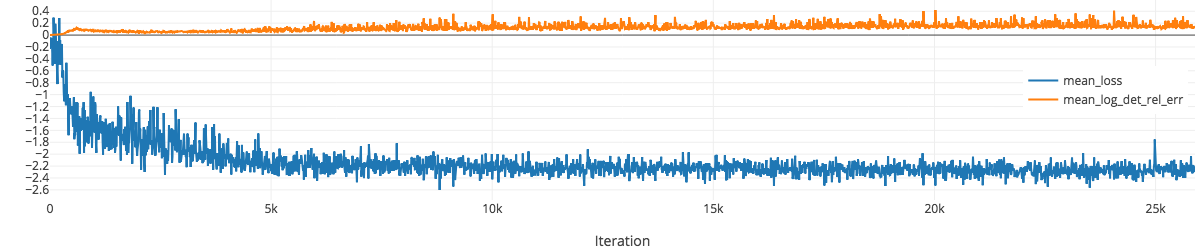
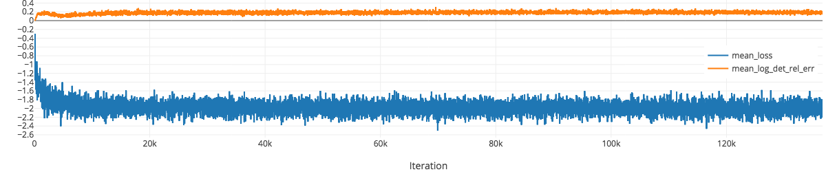
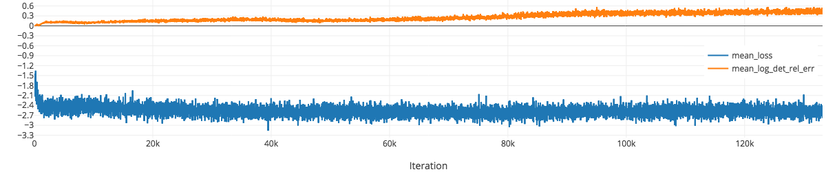
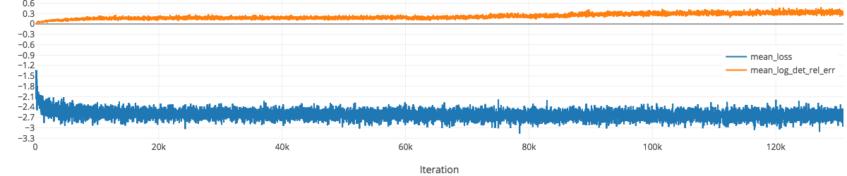
(a)

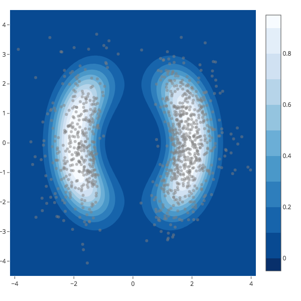
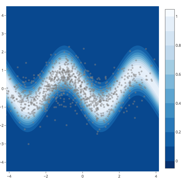
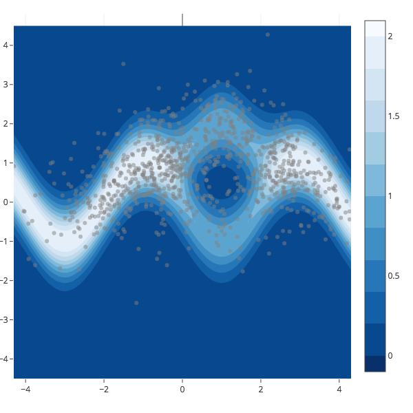
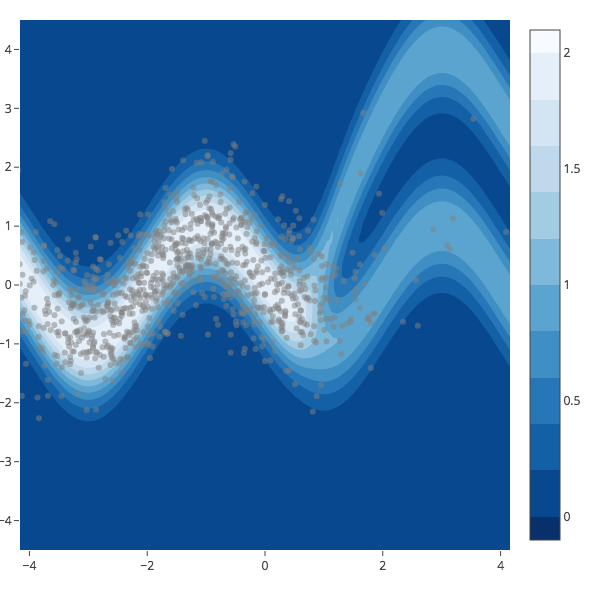
(b)

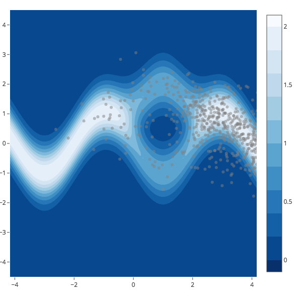
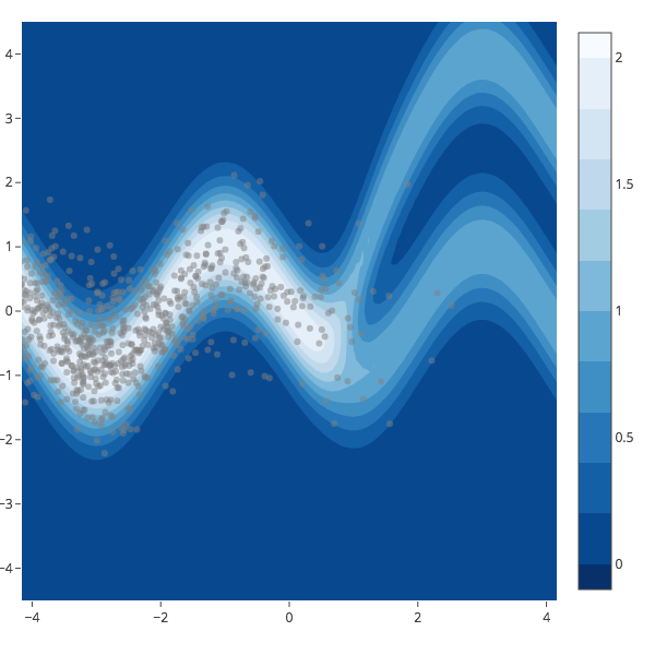
(c)

Figure 1: Results for minimizing $d_{\text{KL}}(Q,P_{X})$ for the four test energies described in Rezende and Mohamed (2015). Subfigures (b) and (c) show the model samples superimposed over contour plots of the corresponding ground-truth test energies. Each epoch corresponds to $5000$ iterations. We see in (a) that the relative error for the approximation to the log determinant typically stays below 30%, except toward the end of training for the last two test energies. At this point, samples from these two models begin to drift away from the origin, as shown in (c).

Suppose that we are tasked with matching a given data distribution $P_{X}$ with the implicit density $Q$ of the model $f$. Two approaches for learning $f$ are available, and the choice of which to use depends on the type of access we have to the data distribution $P_{X}$. The first approach – minimizing $d_{\text{KL}}(Q,P_{X})$ – is applicable when we know how to evaluate the likelihood of $P_{X}$, but are not necessarily able to sample from it. The second approach – minimizing $d_{\text{KL}}(P_{X},Q)$ – is applicable when we are able to sample from $P_{X}$, but are not necessarily able to evaluate its likelihood. We show that spectral backpropagation can be used in both cases, when neither of the two conditions described in Section 1 holds.

All of the examples considered here are densities over $\mathbb{R}^{2}$. We match them by transforming a prior $P_{Z}$ given by a spherical normal distribution. Our choice for the architecture of $f$ is a Wide ResNet comprised of four residual blocks. Each block is a three-layer bottleneck from $\mathbb{R}^{2}$ to $\mathbb{R}^{2}$ whose hidden layer size is 32. All layers are equipped with biases, and use LeakyReLU activations. We compute the gradient updates using a batch size of 64, and apply the updates using Adam (Kingma and Ba, 2014) with a step size of $1\text{\times}{10}^{-4}$, and all other parameters kept at their the default values.

To compute the gradient update given by Equation 3, we use Algorithm 1 with $(m,p,t,g)\coloneqq(10,20,20,1.2)$ for all experiments. For minimizing $d_{\text{KL}}(Q,P_{X})$, we use $\epsilon\coloneqq 0.1$, and for minimizing $d_{\text{KL}}(P_{X},Q)$, $\epsilon\coloneqq$1\text{\times}{10}^{-2}$$. In order to monitor the accuracy of the approximation for the likelihood, we compute $M_{f}$ at each iteration, and evaluate the ground-truth likelihood in accordance with Equation 2. We define the relative error of the approximation $\ln\hat{\ell}$ with respect to the ground-truth log-likelihood $\ln\ell$ by

$$\ln\hat{\ell}-\ln\ell=\ln\frac{\hat{\ell}}{\ell}=\ln\left(1+\frac{\hat{\ell}-\ell}{\ell}\right)\approx\frac{\hat{\ell}-\ell}{\ell},$$

provided that the quotient is not too large. This definition of relative error avoids numerical problems when $\ell\approx 0$.

We begin by considering the first approach, in which we seek to minimize $d_{\text{KL}}(Q,P_{X})$. This objective requires that we be able to sample from $Q$, so we choose $f:Z\to X$ to be a map from latent space to observation space. The results are shown in Figure 1. To prevent $f$ from making $Q$ collapse to model the infinite support of $P_{X}$, we found it helpful to incorporate the regularizer

$$R(M_{f})\coloneqq\rho\|M_{f}\|_{2}$$ (8)

into the objectives for the third and fourth test energies. Here, $\|\cdot\|_{2}$ denotes the spectral norm. To implement this regularizer, we simply backpropagate through the estimate of $\lambda_{\text{max}}$ that is already produced by Algorithm 1. We use $\rho\coloneqq$8\text{\times}{10}^{-2}$$ in both cases. Despite the use of this regularizer, we find that continuing to train the models for these last two test energies causes the samples to drift away from the origin (see Figure 1(c)). We have not made any attempt to address this behavior. Finally, we note that since $d_{\text{KL}}(Q,P_{X})$ is bounded from below by the negative log-normalization constant of $Q$, it can become negative when $Q$ is unnormalized. We see that this happens for all four examples.

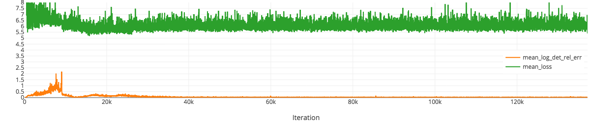
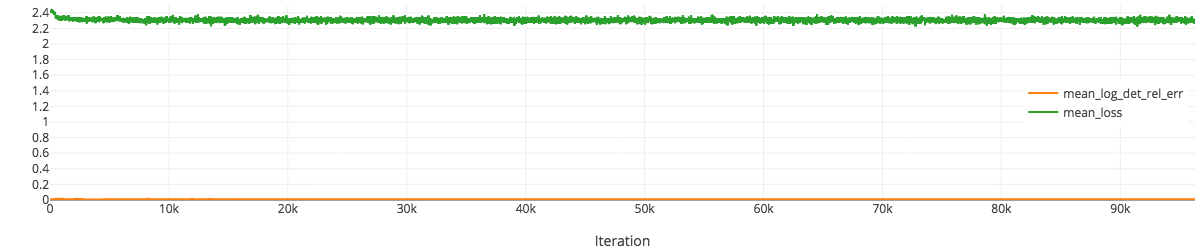
(a)

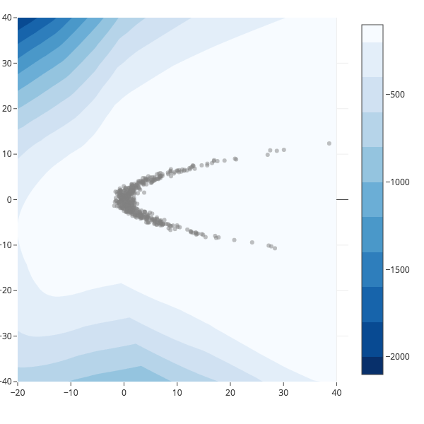
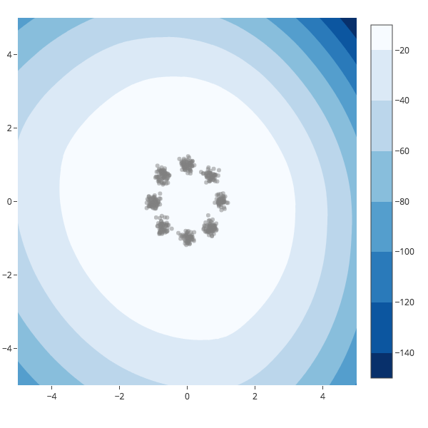
(b)

Figure 2: Results for minimizing $d_{\text{KL}}(P_{X},Q)$ for the crescent and circular mixture densities whose definitions are given in the supplementary material. The relative error for the approximation to the log determinant typically stays below 5%. In (b), we show samples from $P_{X}$ superimposed over contour plots of the log-likelihood of $f$.

In the second approach, we seek to minimize $d_{\text{KL}}(P_{X},Q)$. This objective requires that we be able to evaluate the likelihood of $Q$, so we choose $f:X\to Z$ to be a map from observation space to latent space. The results are shown in Figure 2. We note that minimizing $d_{\text{KL}}(P_{X},Q)$ is ill-posed when $Q$ is unnormalized. In this scenario, the model distribution $Q$ can match $P_{X}$ while also assigning mass outside the support of $P_{X}$. We see that this expected behavior manifests in both examples.

4 Evaluating GAN Likelihoods

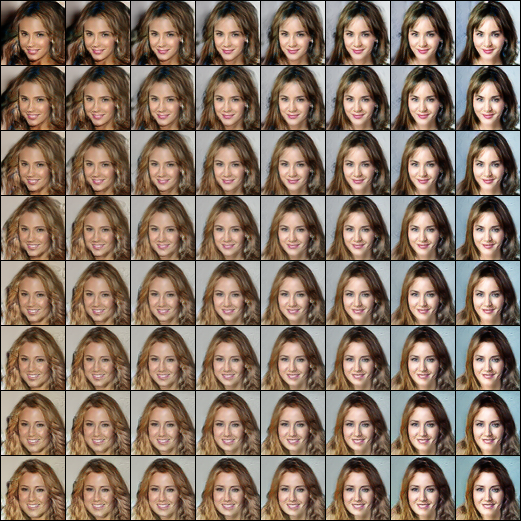
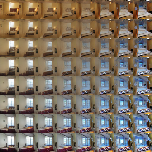
(a)

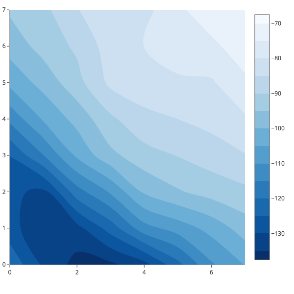
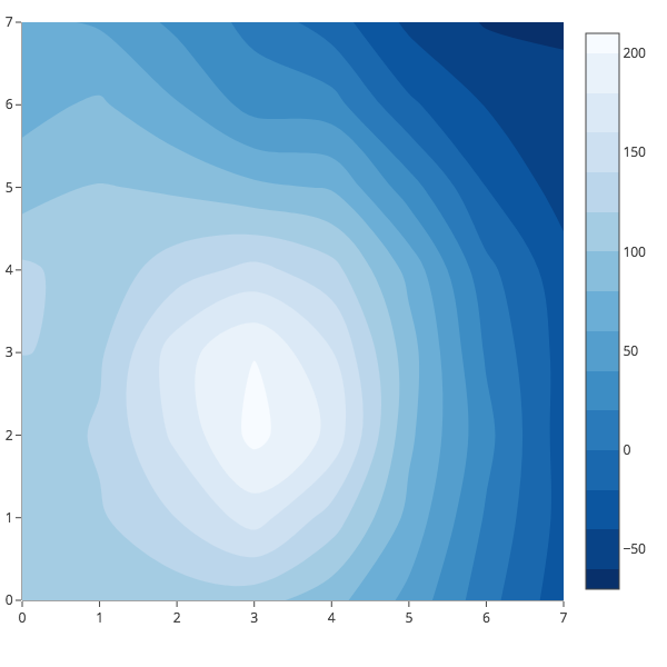
(b)

Figure 3: Samples from two models evaluated at fixed grids in latent space (left), and contour plots of the model log-likelihood evaluated over the same grids (right).

For our explorations involving GANs, we train a series of DCGAN (Radford et al., 2015) models on $64\times 64$ rescaled versions of the CelebA (Liu et al., 2015) and LSUN Bedroom datasets. We vary model capacity in terms of the base feature map count multiplier $n_{f}$ for the DCGAN architecture. The generator and discriminator have five layers each, and use translated LeakyReLU activations (Xiang and Li, 2017). To stabilize training, we use weight normalization with fixed scale factors in the discriminator (Salimans et al., 2016). Our prior is defined by $P_{Z}\coloneqq\operatorname{unif}([-1,1])^{n_{z}}$, where $n_{z}$ is the size of the embedding space. All models were trained for $750\,000$ iterations with a batch size of 32, using RMSProp with step size $1\text{\times}{10}^{-4}$ and decay factor $0.9$. We present results from two of these models in Figure 3.

(a)

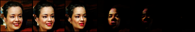
(b)

(c)

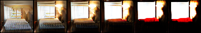
(d)

Trial	${\log(p_{\text{final}}/p_{\text{init}})}$	Initial $(\lambda_{\text{min}},\lambda_{\text{max}})$	Final $(\lambda_{\text{min}},\lambda_{\text{max}})$	$(m,p,t,g,\epsilon)$
(a)	$161.400\,787\,353\,515\,62$	$($0.231\,203\,32$,$2907.4229$)$	$($0.008\,105\,371$,$1059.2062$)$	$(5,20,20,1.1,$1\text{\times}{10}^{-4}$)$
(b)	$667.431\,869\,506\,835\,9$	$($0.270\,956\,07$,$2233.8276$)$	$($2.514\,679\,4\text{\times}{10}^{-06}$,$0.257\,371\,28$)$	$(5,20,20,1.1,$1\text{\times}{10}^{-5}$)$
(c)	$90.825\,170\,516\,967\,77$	$($0.018\,747\,492$,$1995.3479$)$	$($0.008\,580\,686$,$562.2244$)$	$(5,10,10,1.2,$1\text{\times}{10}^{-2}$)$
(d)	$336.068\,625\,450\,134\,3$	$($0.022\,936\,836$,$1242.7954$)$	$($0.000\,611\,809\,9$,$403.832\,06$)$	$(5,10,10,1.2,$1\text{\times}{10}^{-2}$)$

Figure 4: Trajectories of four latent variables as they are perturbed to optimize likelihood under the generator. Trajectories (a) and (b) correspond to the CelebA model with $n_{z}=128,n_{f}=64$, and trajectories (c) and (d) to the LSUN Bedroom model with $n_{z}=256,n_{f}=64$. Statistics from these trajectories are tabulated above. The last column of the table specifies the parameters used for Algorithm 1 to compute the gradient estimates.

We apply spectral backpropagation to explore the effect of perturbing a given latent variable $z\in Z$ to maximize likelihood under the generator distribution $Q$. This is readily accomplished by noting that the same procedure to evaluate Equation 3 can also be used to obtain gradients with respect to $z$. The results are shown in Figure 4. Intuitively, we might expect the outputs to be transformed in such a way that they gravitate towards modes of the dataset. But this is not what happens. Instead, the outputs are transformed into highly aberrant, out-of-distribution examples while nonetheless attaining very high likelihood. As optimization proceeds, $M_{f}$ also becomes increasingly ill-conditioned. This shows that likelihood for generators need not correspond to intuitive notions of visual plausibility.

5 Uncovering Latent Explanatory Factors

(a)

(b)

(c)

(d)

(e)

(f)

(g)

(h)

Figure 5: Result of perturbing latent variables along the eigenvectors of $M_{f}$. In (a) and (b), we show the top eigenvalues of $\operatorname{Sp}(M_{f})$ evaluated at 12 trial latent variables. Small eigenvalues are not shown. The leftmost images of each grid both contain duplicates of the original, each corresponding one of the 12 latent variables. The top row shows the effect of applying perturbations along random directions, and the bottom row the result of applying perturbations with the same step size along the eigenvectors.

The generator in GANs is well-known for organizing latent space such that semantic features can be transferred by means of algebraic operations over latent variables (Radford et al., 2015). This suggests the existence of a systematic organization of latent space, but perhaps one that cannot be globally characterized in terms of a handful of simple explanatory factors. We instead explore whether local changes in latent space can be characterized in this way. Since the metric $M_{f}$ describes local change in the generator’s output, it is natural to consider the effect of perturbations along its eigenvectors. To this end, we fix 12 trial embeddings in latent space, and compare the effect of perturbations along random directions to perturbations along these eigenvectors. The random directions are obtained by sampling from a spherical normal distribution. We show the results in Figure 5.

We can see that dominant eigenvalues, especially the principal eigenvalue, often result in the most drastic changes. Furthermore, these changes are not only semantically meaningful, but also tend to make modifications to distinct attributes of the image. To see this more clearly, we consider the top two rows of Figure 5(g). Movement along the first two eigenvectors changes hair length and facial orientation; movement along the third eigenvector decreases the length of the bangs; movement along the fourth and fifth eigenvectors changes background color; and movement along the sixth and seventh eigenvectors changes hair color.

(a)

(b)

(c)

(d)

Dataset	$v_{\text{eff}}(\tau=1)$ for ${n_{f}}$ fixed, ${n_{z}}$ varied			$v_{\text{eff}}(\tau=1)$ for ${n_{z}}$ fixed, ${n_{f}}$ varied
	${(n_{z}/2,n_{f})}$	${(n_{z},n_{f})}$	${(2n_{z},n_{f})}$	${(n_{z},n_{f}/2)}$	${(n_{z},n_{f})}$	${(n_{z},2n_{f})}$
CelebA ($n_{z}=64,n_{f}=64$)	$6.949\,218\,75$	$10.492\,187\,5$	$16.550\,781\,25$	$16.140\,625$	$16.550\,781\,25$	$17.285\,156\,25$
LSUN Bedroom ($n_{z}=64,n_{f}=128$)	$25.226\,562\,5$	$34.929\,687\,5$	$53.601\,562\,5$	$28.367\,187\,5$	$34.929\,687\,5$	$40.042\,968\,75$

(e)

Figure 6: Effect of varying $n_{z}$ and $n_{f}$ on $v_{\text{eff}}(\tau)$. Plots (a)–(d) show $v_{\text{eff}}$ as a function of $\tau$. Larger values for $v_{\text{eff}}$ suggest increased utilization of latent space. Table (e) shows that doubling $n_{z}$ roughly doubles $v_{\text{eff}}$. On the other hand, doubling $n_{f}$ does not result in noticeable change for CelebA, and only results in a modest increase in $v_{\text{eff}}$ for LSUN Bedroom. The step sizes used for the perturbations are the same as those reported in Figure 5.

Inspecting the two columns (c), (e), (g), and (d), (f), (h) in Figure 5 suggests that larger values of $n_{z}$ may encourage the generator to capture more explanatory factors, possibly at the price of decreased sample quality. We would like to explore the effect of varying $n_{z}$ and $n_{f}$ on the number of such factors. To do this, we fix a sample of latent variables $S\coloneqq\{z_{j}\}_{j\in[1,M]}\sim P_{Z}$. For each $z_{j}\in S$, we define

$$\delta(j,0)\coloneqq\operatorname{E}_{\epsilon\sim N(0,I)}\|G(z_{j}+\alpha\epsilon)-G(z_{j})\|_{2}\quad\text{and}\quad\delta(j,i)\coloneqq\frac{\|G(z_{j}+\alpha v_{i}^{(j)})-G(z_{j})\|_{2}}{\delta(j,0)},$$

for every eigenvector $v_{1}^{(j)},\ldots,v_{n_{z}}^{(j)}$ of $M_{f}(z_{j})$. The quantity $\delta(j,i)$ measures the pixelwise change resulting from a perturbation along an eigenvector, relative to the change we expect from a random perturbation. Finally, we define

$$v_{\text{eff}}(\tau)\coloneqq\frac{1}{M}\sum_{j\in[1,M]}\sum_{i\in[1,n_{z}]}1\{\delta(j,i)>\tau\},$$

where $1\{\cdot\}$ is the indicator function. This quantity measures the average number of eigenvectors for which the relative change is greater than the threshold $\tau$. As such, it can be regarded as an effective measure of dimensionality for latent space. We explore the effect of varying $n_{z}$ and $n_{f}$ on $v_{\text{eff}}$ in Figure 6.

6 Conclusion

Current approaches for probabilistic modeling attempt to satisfy two goals that are fundamentally at odds with one another: fulfillment of the two constraints described in Section 1, and model flexibility. In this work, we develop a computational tool that aims to expand the scope of probabilistic modeling to functions that do not satisfy these constraints. We make the first steps toward demonstrating feasibility of this approach by minimizing divergences in far greater generality than what has been attempted before. Finally, we uncover surprising facts about the organization of latent space for GANs that we hope will contribute to an improved understanding of how effectively they capture underlying latent structure.

References

- Abadi et al. [2016] Martín Abadi, Paul Barham, Jianmin Chen, Zhifeng Chen, Andy Davis, Jeffrey Dean, Matthieu Devin, Sanjay Ghemawat, Geoffrey Irving, Michael Isard, et al. Tensorflow: A system for large-scale machine learning. In OSDI, volume 16, pages 265–283, 2016.
- Avron and Toledo [2011] Haim Avron and Sivan Toledo. Randomized algorithms for estimating the trace of an implicit symmetric positive semi-definite matrix. Journal of the ACM (JACM), 58(2):8, 2011.
- Berg et al. [2018] Rianne van den Berg, Leonard Hasenclever, Jakub M Tomczak, and Max Welling. Sylvester normalizing flows for variational inference. arXiv preprint arXiv:1803.05649, 2018.
- Boutsidis et al. [2017] Christos Boutsidis, Petros Drineas, Prabhanjan Kambadur, Eugenia-Maria Kontopoulou, and Anastasios Zouzias. A randomized algorithm for approximating the log determinant of a symmetric positive definite matrix. Linear Algebra and its Applications, 533:95–117, 2017.
- Dinh et al. [2016] Laurent Dinh, Jascha Sohl-Dickstein, and Samy Bengio. Density estimation using real nvp. arXiv preprint arXiv:1605.08803, 2016.
- Fitzsimons et al. [2017] Jack Fitzsimons, Diego Granziol, Kurt Cutajar, Michael Osborne, Maurizio Filippone, and Stephen Roberts. Entropic trace estimates for log determinants. In Joint European Conference on Machine Learning and Knowledge Discovery in Databases, pages 323–338. Springer, 2017.
- Germain et al. [2015] Mathieu Germain, Karol Gregor, Iain Murray, and Hugo Larochelle. Made: Masked autoencoder for distribution estimation. In International Conference on Machine Learning, pages 881–889, 2015.
- Goodfellow et al. [2014] Ian Goodfellow, Jean Pouget-Abadie, Mehdi Mirza, Bing Xu, David Warde-Farley, Sherjil Ozair, Aaron Courville, and Yoshua Bengio. Generative adversarial nets. In Advances in neural information processing systems, pages 2672–2680, 2014.
- Han et al. [2017] Insu Han, Dmitry Malioutov, Haim Avron, and Jinwoo Shin. Approximating spectral sums of large-scale matrices using stochastic chebyshev approximations. SIAM Journal on Scientific Computing, 39(4):A1558–A1585, 2017.
- Hanson [1994] Andrew J. Hanson. Graphics gems iv. chapter Geometry for N-dimensional Graphics, pages 149–170. Academic Press Professional, Inc., San Diego, CA, USA, 1994. ISBN 0-12-336155-9. URL http://dl.acm.org/citation.cfm?id=180895.180909.
- Hutchinson [1990] Michael F Hutchinson. A stochastic estimator of the trace of the influence matrix for laplacian smoothing splines. Communications in Statistics-Simulation and Computation, 19(2):433–450, 1990.
- Jang [2018] Eric Jang. Normalizing flows tutorial, part 2: Modern normalizing flows, 2018. URL https://blog.evjang.com/2018/01/nf2.html.
- Kingma and Ba [2014] Diederik P Kingma and Jimmy Ba. Adam: A method for stochastic optimization. arXiv preprint arXiv:1412.6980, 2014.
- Kingma and Welling [2013] Diederik P Kingma and Max Welling. Auto-encoding variational bayes. arXiv preprint arXiv:1312.6114, 2013.
- Kingma et al. [2016] Diederik P Kingma, Tim Salimans, Rafal Jozefowicz, Xi Chen, Ilya Sutskever, and Max Welling. Improved variational inference with inverse autoregressive flow. In Advances in Neural Information Processing Systems, pages 4743–4751, 2016.
- Krantz and Parks [2008] Steven Krantz and Harold Parks. Analytical tools: The area formula, the coarea formula, and poincaré inequalities. Geometric Integration Theory, pages 1–33, 2008.
- Li and Turner [2017] Yingzhen Li and Richard E Turner. Gradient estimators for implicit models. arXiv preprint arXiv:1705.07107, 2017.
- Liu et al. [2015] Ziwei Liu, Ping Luo, Xiaogang Wang, and Xiaoou Tang. Deep learning face attributes in the wild. In Proceedings of International Conference on Computer Vision (ICCV), 2015.
- Neal [2001] Radford M Neal. Annealed importance sampling. Statistics and computing, 11(2):125–139, 2001.
- Papamakarios et al. [2017] George Papamakarios, Iain Murray, and Theo Pavlakou. Masked autoregressive flow for density estimation. In Advances in Neural Information Processing Systems, pages 2335–2344, 2017.
- Paszke et al. [2017] Adam Paszke, Sam Gross, Soumith Chintala, Gregory Chanan, Edward Yang, Zachary DeVito, Zeming Lin, Alban Desmaison, Luca Antiga, and Adam Lerer. Automatic differentiation in pytorch. 2017.
- Radford et al. [2015] Alec Radford, Luke Metz, and Soumith Chintala. Unsupervised representation learning with deep convolutional generative adversarial networks. arXiv preprint arXiv:1511.06434, 2015.
- Rezende and Mohamed [2015] Danilo Jimenez Rezende and Shakir Mohamed. Variational inference with normalizing flows. arXiv preprint arXiv:1505.05770, 2015.
- Rezende et al. [2014] Danilo Jimenez Rezende, Shakir Mohamed, and Daan Wierstra. Stochastic backpropagation and approximate inference in deep generative models. arXiv preprint arXiv:1401.4082, 2014.
- Salimans et al. [2016] Tim Salimans, Ian Goodfellow, Wojciech Zaremba, Vicki Cheung, Alec Radford, and Xi Chen. Improved techniques for training gans. In Advances in Neural Information Processing Systems, pages 2234–2242, 2016.
- Szegedy et al. [2013] Christian Szegedy, Wojciech Zaremba, Ilya Sutskever, Joan Bruna, Dumitru Erhan, Ian Goodfellow, and Rob Fergus. Intriguing properties of neural networks. arXiv preprint arXiv:1312.6199, 2013.
- Tomczak and Welling [2016] Jakub M Tomczak and Max Welling. Improving variational auto-encoders using householder flow. arXiv preprint arXiv:1611.09630, 2016.
- Ubaru et al. [2017] Shashanka Ubaru, Jie Chen, and Yousef Saad. Fast estimation of tr(f(a)) via stochastic lanczos quadrature. SIAM Journal on Matrix Analysis and Applications, 38(4):1075–1099, 2017.
- van den Oord et al. [2016a] Aaron van den Oord, Sander Dieleman, Heiga Zen, Karen Simonyan, Oriol Vinyals, Alex Graves, Nal Kalchbrenner, Andrew Senior, and Koray Kavukcuoglu. Wavenet: A generative model for raw audio. arXiv preprint arXiv:1609.03499, 2016a.
- van den Oord et al. [2016b] Aaron van den Oord, Nal Kalchbrenner, Lasse Espeholt, Oriol Vinyals, Alex Graves, et al. Conditional image generation with pixelcnn decoders. In Advances in Neural Information Processing Systems, pages 4790–4798, 2016b.
- van den Oord et al. [2016c] Aaron van den Oord, Nal Kalchbrenner, and Koray Kavukcuoglu. Pixel recurrent neural networks. arXiv preprint arXiv:1601.06759, 2016c.
- van den Oord et al. [2017] Aaron van den Oord, Yazhe Li, Igor Babuschkin, Karen Simonyan, Oriol Vinyals, Koray Kavukcuoglu, George van den Driessche, Edward Lockhart, Luis C Cobo, Florian Stimberg, et al. Parallel wavenet: Fast high-fidelity speech synthesis. arXiv preprint arXiv:1711.10433, 2017.
- Wu et al. [2016] Yuhuai Wu, Yuri Burda, Ruslan Salakhutdinov, and Roger Grosse. On the quantitative analysis of decoder-based generative models. arXiv preprint arXiv:1611.04273, 2016.
- Xiang and Li [2017] Sitao Xiang and Hao Li. On the effects of batch and weight normalization in generative adversarial networks. stat, 1050:22, 2017.
- Zagoruyko and Komodakis [2016] Sergey Zagoruyko and Nikos Komodakis. Wide residual networks. arXiv preprint arXiv:1605.07146, 2016.