Bandwidth selection for kernel density estimators of multivariate level sets and highest density regions

Abstract

We consider bandwidth matrix selection for kernel density estimators (KDEs) of density level sets in $\mathbb{R}^{d}$, $d\geq 2$. We also consider estimation of highest density regions, which differs from estimating level sets in that one specifies the probability content of the set rather than specifying the level directly. This complicates the problem. Bandwidth selection for KDEs is well studied, but the goal of most methods is to minimize a global loss function for the density or its derivatives. The loss we consider here is instead the measure of the symmetric difference of the true set and estimated set. We derive an asymptotic approximation to the corresponding risk. The approximation depends on unknown quantities which can be estimated, and the approximation can then be minimized to yield a choice of bandwidth, which we show in simulations performs well. We provide an R package lsbs for implementing our procedure.

1 Introduction

As computing power has become greater and as data sets have become simultaneously larger and more complicated, demand for statistical methods that are increasingly flexible and data driven has increased. Two related methods for capturing the complex structure of a data set from a true density $f_{0}$ are to estimate either the density’s level sets (LS’s) or the density’s highest-density regions (HDR’s). (We will explain the difference between estimating LS’s and estimating HDR’s shortly.) For a density function $f_{0}$ defined on $\mathbb{R}^{d}$ and a given constant $c>0$, the $c$-level set (sometimes known as a density contour) of $f_{0}$ is $\beta(c):=\{\boldsymbol{x}\in\mathbb{R}^{d}:f_{0}(\boldsymbol{x})=c\},$ and the corresponding super-level set is

$$\mathcal{L}(c):=\{\boldsymbol{x}\in\mathbb{R}^{d}:f_{0}(\boldsymbol{x})\geq c\}.$$ (1)

Under some basic regularity conditions, the density super-level set is a set of minimum volume having $f_{0}$-probability at least $\int_{\mathcal{L}(c)}f_{0}(\boldsymbol{x})\,d\boldsymbol{x}$ (Garcia et al., 2003). For this reason, perhaps the most common use for HDR estimation occurs in Bayesian statistics. An HDR of a posterior density is a so-called (minimum volume) credible region, which is one of the most fundamental tools in Bayesian statistics. There are quite a wide range of other applications for estimation of density LS’s or density HDR’s and these estimation problems have received increasing attention in the statistics and machine learning literatures in recent years. (We consider estimation of density level sets and estimation of density super-level sets to be equivalent tasks.) The applications of LS or HDR estimation include outlier/novelty detection (Lichman and Smyth, 2014; Park et al., 2010), discriminant analysis (Mammen and Tsybakov, 1999) and clustering analysis (Hartigan, 1975; Rinaldo and Wasserman, 2010; Cuevas et al., 2001). LS estimation is one of the fundamental tools in estimation of cluster trees and persistence diagrams, used in topological data analysis (Chen (2017), Wasserman (2016)).

A common way to estimate the density super-level set $\mathcal{L}(c)$ based on independent and identically distributed (i.i.d.) $\boldsymbol{X}_{1},\ldots,\boldsymbol{X}_{n}\in\mathbb{R}^{d}$ is to replace the density function in (1) with a kernel density estimator (KDE)

$$\widehat{f}_{n,\boldsymbol{H}}(\boldsymbol{x}):=\frac{1}{n}\sum_{i=1}^{n}K(\boldsymbol{H}^{-1/2}(\boldsymbol{x}-\boldsymbol{X}_{i}))|\boldsymbol{H}|^{-1/2},$$ (2)

where $\boldsymbol{H}\in\mathbb{R}^{d\times d}$ is a symmetric positive definite bandwidth matrix and $K$ is a kernel function. This gives us the so-called plug-in estimator

$$\widehat{\mathcal{L}}_{n,\boldsymbol{H}}(c):=\{\boldsymbol{x}\in\mathbb{R}^{d}:\widehat{f}_{n,\boldsymbol{H}}(\boldsymbol{x})\geq c\}.$$ (3)

We now explain the difference between “LS estimation” and “HDR estimation.” Often the level of interest is only specified indirectly through a given probability $\tau\in(0,1)$ which yields a level $f_{\tau,0}:=\inf\{y>0:\int_{\mathbb{R}^{d}}f_{0}(\boldsymbol{x})\mathbbm{1}_{\{f(\boldsymbol{x})\geq y\}}\,d\boldsymbol{x}\leq 1-\tau\}$. Then the corresponding super-level set is

$$\mathcal{L}(f_{\tau,0}):=\{\boldsymbol{x}\in\mathbb{R}^{d}:f_{0}(\boldsymbol{x})\geq f_{\tau,0}\},$$ (4)

and the corresponding plug-in estimators are

$$\hat{f}_{\tau,n}:=\inf\left\{y\in(0,\infty):\int_{\mathbb{R}^{d}}\widehat{f}_{n,\boldsymbol{H}}(\boldsymbol{x})\mathbbm{1}_{\{\widehat{f}_{n,\boldsymbol{H}}(\boldsymbol{x})\geq y\}}\,d\boldsymbol{x}\leq 1-\tau\right\}$$

and

$$\widehat{\mathcal{L}}_{n,\boldsymbol{H}}(\hat{f}_{\tau,n}):=\{\boldsymbol{x}\in\mathbb{R}^{d}:\widehat{f}_{n,\boldsymbol{H}}(\boldsymbol{x})\geq\hat{f}_{\tau,n}\}.$$ (5)

Estimating (4) based on specifying $\tau$ is known as the HDR estimation problem; this has extra complication over the LS estimation problem because $f_{\tau,0}$ has to be estimated rather than being fixed in advance. Thus we use the phrase LS estimation to mean estimation of (1) with $c$ fixed in advance (equivalently, estimation of (4) with $f_{\tau,0}$ fixed). When we use the phrase HDR estimation we mean estimation of (4) with $\tau$ (but not $f_{\tau,0}$) fixed in advance. Thus, LS’s and HDR’s are mathematically equivalent, but estimating LS’s and estimating HDR’s are statistically different tasks.

Early work on LS or HDR estimation includes Hartigan (1987), Müller and Sawitzki (1991), Polonik (1995), Tsybakov (1997), and Walther (1997). Some recent work has focused on asymptotic properties of KDE plug-in estimators, including results about consistency, limit distribution theory, and statistical inference. Baíllo et al. (2001) show that the probability content of the plug-in estimator converges to the probability of the true super-level set as the sample size tends to infinity. Baíllo (2003) proves the strong consistency of the plug-in estimator under an integrated symmetric difference metric. Cadre (2006) further obtains the rate of convergence of the plug-in estimator when the loss is given by the generalized symmetric difference of sets. Mason and Polonik (2009) give the asymptotic normality of estimated super-level sets under the same metric as Cadre (2006). Chen et al. (2017) find a more practically usable limiting distribution of the plug-in estimator for LS’s by using Hausdorff distance as the metric for set difference and provide methods for constructing confidence regions for LS’s based on this limiting distribution. Jankowski and Stanberry (2012) and Mammen and Polonik (2013) also investigate the formation of confidence regions for LS’s.

It is well known that KDE’s are sensitive to the choice of the bandwidth (matrix). The optimal bandwidth (matrix) depends on the objective of estimation. There are many tools that have been developed for selecting the bandwidth when $d=1$ or the bandwidth matrix when $d>1$; these include minimizing an asymptotic approximation to an appropriate risk function, as well as computational methods such as the bootstrap or cross-validation, and are largely focused on globally estimating the density or its derivatives well. A good summary of those methods can be found in Wand and Jones (1995), Sain et al. (1994b), or Jones et al. (1996).

However, Duong et al. (2009, page 505) state that, “a number of practical issues in highest density region estimation, such as good data-driven rules for choosing smoothing parameters, are yet to be resolved.” Samworth and Wand (2010) is the only published work we know of that investigates the problem of selecting bandwidths for HDR estimation (and we know of no published works that directly investigate bandwidth selection for LS estimation). Samworth and Wand (2010) study the KDE plug-in estimator when $d=1$, and show by simulation that the kernel density estimator aiming for HDR estimation can be very different from the one aiming for global density estimation. They also propose an asymptotic approximation to a risk function that is suitable for HDR estimation and a corresponding bandwidth selection procedure based on the approximation, all when $d=1$.

In this paper, we consider the multivariate setting, where $d\geq 2$. In this case, we are estimating a level set manifold, which involves some added technical difficulties over the case $d=1$ (in which case the level set is a finite point set), but we believe that LS or HDR estimation when $d\geq 2$ is of great practical interest because of the large variety of complicated structures that multivariate level sets can reveal. We derive asymptotic approximations to a risk function for LS estimation and to a risk function for HDR estimation. We believe that our approximations and derivations will be very valuable for any future procedures that do (either) LS or HDR bandwidth selection. Our calculations shed light on the important quantities relating to LS or HDR estimation. Furthermore, we develop a “plug-in” bandwidth selector method based on minimizing an estimate of the LS or the HDR risk approximation. This approach can be used to optimize over all positive definite bandwidth matrices or over restricted classes of matrices (e.g., diagonal ones). Our theory applies for all $d\geq 2$. We have developed code to implement our bandwidth selector when $d=2$. It is straightforward to implement a numeric approximation to Hausdorff integrals that appear in our approximations (see Subsection 2.1 for discussion of the Hausdorff measure) when $d=2$. It is less immediately obvious how to implement such approximations when $d\geq 3$, although we indeed believe that implementation is feasible for such approximations. In fact, we believe that computational feasibility is an important benefit of using a closed-form approximation to the risk, particularly in the multivariate setting that we consider in this paper. As will be discussed later in the paper, many simple problems in the univariate setting are more complicated in the multivariate setting and must be solved by Monte Carlo. Thus performing bootstrap or cross-validation, which involves nested Monte Carlo computations, quickly becomes infeasible.

During the development of the present paper we became aware of the recent related work, Qiao (2018). Qiao (2018) also considers problems about bandwidth selection for KDE’s in settings related to level set estimation. However, the main focus of Qiao (2018) is somewhat different than the one here. In fact, Qiao (2018) states that bandwidth selection for multivariate HDR estimation is “far from trivial” and does not consider this problem. We will discuss the approach taken by Qiao (2018) again in the Discussion section.

The structure of the paper is as follows. We present our two asymptotic risk approximation theorems, as well as corollaries about the risk approximation minimizers, in Section 2. We present methodology to select bandwidth matrices in Section 3. In Section 4 we study the performance of our bandwidth selector in simulation experiments as well as in analysis of two real data sets, the Wisconsin Breast Cancer Diagnostic data and the Banknote Authentication data. We give concluding discussion in Section 5. Proofs of the main results are given in Appendix A, and further details, technical results, and intermediate lemmas are given in Appendix B and Appendix C. Some notation and assumptions are presented in Subsections 2.1 and 2.2.

2 Asymptotic risk results

2.1 Notation

We use the following notation throughout. For a density function $f_{0}$ on $\mathbb{R}^{d}$ and a Borel measurable set $A\subset\mathbb{R}^{d}$, define the measure $\mu_{f_{0}}(A)=\int_{A}f_{0}(\boldsymbol{x})\,d\boldsymbol{x}$. For a function $f$ on $\mathbb{R}^{d}$, a measure $P$, and $1\leq p<\infty$, we let $\|f\|_{p,P}^{p}=\int_{\mathbb{R}^{d}}|f(\boldsymbol{z})|^{p}dP(\boldsymbol{z})$ if this quantity is finite. If $P$ is Lebesgue measure we abbreviate $\|f\|_{p,P}\equiv\|f\|_{p}$, $1\leq p<\infty$. Let $\|f\|_{\infty}=\sup_{\boldsymbol{z}\in\mathbb{R}^{d}}|f(\boldsymbol{z})|$, and for a function $g$ with vector or matrix values, that is, $g:\mathbb{R}^{d}\rightarrow\mathbb{R}^{p\times q}$, let $\|g\|_{\infty}=\max_{1\leq i\leq p,1\leq j\leq q}\|g_{ij}\|_{\infty}$. We let $\|{\boldsymbol{x}}\|=(\sum_{i=1}^{d}x_{i}^{2})^{1/2}$ for $\boldsymbol{x}\in\mathbb{R}^{d}$. Let $\nabla f$ be the gradient (column) vector of $f$ and let $\nabla^{2}f$ be the Hessian matrix $\left(\frac{\partial^{2}f}{\partial x_{i}\partial x_{j}}\right)_{i,j}$. Let $\mathcal{H}$ be $d-1$ dimensional Hausdorff measure (Evans and Gariepy, 2015). The Hausdorff measure is useful for measuring the volume of lower dimensional sets, like manifolds, embedded in a higher dimensional ambient space. Let $\lambda$ denote Lebesgue measure. Recall that $\beta(c):=\{\boldsymbol{x}\in\mathbb{R}^{d}:f_{0}(\boldsymbol{x})=c\}$ and $\mathcal{L}(c):=\{\boldsymbol{x}\in\mathbb{R}^{d}:f_{0}(\boldsymbol{x})\geq c\}$, we let $\mathcal{L}_{\tau}\equiv\mathcal{L}(f_{\tau,0})$ and $\widehat{\mathcal{L}}_{\tau,\boldsymbol{H}}\equiv\widehat{\mathcal{L}}_{\boldsymbol{H}}(\widehat{f}_{\tau,n})$. We generally use bold to denote vectors. We use “$\equiv$” to denote notational equivalences and “$:=$” or “$=:$” for definitions. Any integral whose domain is not specified explicitly is taken over all of $\mathbb{R}^{d}$. We will occasionally omit the integrating variable when there’s no confusion in doing so. We use $\mathcal{S}$ to denote the set of all $d\times d$ symmetric positive definite matrices. For a symmetric matrix $\boldsymbol{A}$, we use $\lambda_{\max}(\boldsymbol{A})$ and $\lambda_{\min}(\boldsymbol{A})$ to denote the largest and the smallest eigenvalues of $\boldsymbol{A}$ respectively. In this paper, we will use the $f_{0}$-probability volume of the symmetric difference as the distance between the true set and its estimator. We use $\Delta$ to denote the symmetric difference operation between two sets: for two sets $A$ and $B$, $A\Delta B:=(A\cup B)\setminus(A\cap B)$ where “$\setminus$” is set difference. Figure 1 shows the symmetric difference between the $0.02$ super-level set of standard bivariate normal distribution and an “estimated” super-level set. We let $A^{c}$ be the complement of a set $A$. For $\delta>0$ and $\boldsymbol{x}\in\mathbb{R}^{d}$, let $B(\boldsymbol{x},\delta):=\left\{\boldsymbol{y}\in\mathbb{R}^{d}\colon\|\boldsymbol{y}-\boldsymbol{x}\|\leq\delta\right\}$, and for a set $A$, let $A^{\delta}:=\cup_{\boldsymbol{x}\in A}B(\boldsymbol{x},\delta)$.

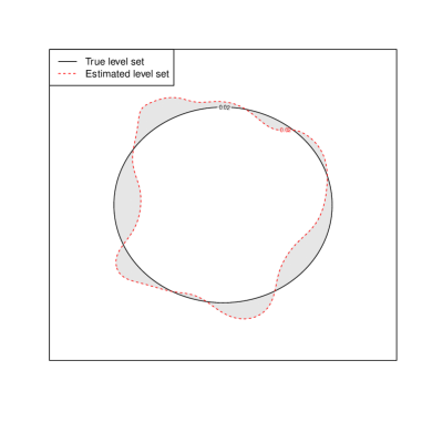
Figure 1: Symmetric difference between the true level set and an estimated level set. The solid black line is the boundary of the true level set and the dashed red line is the boundary of the estimated level set. The shaded area is the symmetric difference of the two sets.

2.2 Assumptions

To derive our asymptotic expansion, we make the following basic assumptions on the underlying density, kernel function and bandwidth matrix.

Assumption D1a.

      

1. Let ${\boldsymbol{X}}_{1},\ldots,\boldsymbol{X}_{n}$ be i.i.d. from a bounded density $f_{0}$ on $\mathbb{R}^{d}$, $d\geq 2$.

2. Fix $\inf_{x\in\mathbb{R}^{d}}f_{0}(x)<c<\|f_{0}\|_{\infty}$. There exists a constant $a>0$ such that (a) $f_{0}$has two bounded continuous partial derivatives over $U_{a}:=\{\boldsymbol{x}:c-a\leq f_{0}(\boldsymbol{x})\leq c+a\}$, (b) $\inf_{U_{a}}\|\nabla f_{0}\|>0$, and (c) $U_{a}$is contained in $\beta(c)^{\delta}$ for some $\delta>0$.

Assumption D1b.

      

1. Let ${\boldsymbol{X}}_{1},\ldots,\boldsymbol{X}_{n}$ be i.i.d. from a bounded density $f_{0}$ on $\mathbb{R}^{d}$, $d\geq 2$.

2. The density $f_{0}$ has two bounded continuous partial derivatives for all $\boldsymbol{x}\in\mathbb{R}^{d}$.

3. There exists a constant $a>0$ such that $U_{a}:=\{\boldsymbol{x}:f_{\tau,0}-a\leq f_{0}(\boldsymbol{x})\leq f_{\tau,0}+a\}$ satisfies (a) $\inf_{U_{a}}\|\nabla f_{0}\|>0$, and (b) $U_{a}$is contained in $\beta_{\tau}^{\delta}$ for some $\delta>0$.

4. For any $c>0$, $\lambda(\{\boldsymbol{x}\in\mathbb{R}^{d}:f_{0}(\boldsymbol{x})=c\})=0$, where $\lambda$ is the Lebesgue measure in $\mathbb{R}^{d}$. (indicated by 3, see NunezGarcia:2003ci)

Assumption Assumption D1a will be used for LS estimation and Assumption Assumption D1b for HDR estimation. We need the stronger global twice differentiability assumption in HDR estimation because of the need to estimate $f_{\tau,0}$ (which involves estimating the $f_{0}$-probability content of $\mathcal{L}_{\tau}$). The global twice differentiability assumption in Assumption Assumption D1b could be weakened to an assumption of twice differentiability either on $\mathcal{L}_{\tau}^{\delta}$ or on $(\mathcal{L}_{\tau}^{c})^{\delta}$.

Assumptions Assumption D1a and Assumption D1b entail that the gradient of $f_{0}$ is nonzero on (a neighborhood of) the level set of interest. This implies by the preimage theorem that the level set $\beta$, taken to be either $\beta(c)$ or $\beta_{\tau}$, is a $(d-1)$-dimensional (boundaryless) manifold (Guillemin and Pollack, 1974). The only additional assumption we need is one of compactness, which rules out only very pathological cases, where $f_{0}$ has “spikes” of increasingly small width going out towards infinity.

Assumption D2.

Let $\inf_{x\in\mathbb{R}^{d}}f_{0}(x)<c<\|f_{0}\|_{\infty}$ or $0<\tau<1$ be as in Assumptions Assumption D1a and Assumption D1b. Assume that $\beta(c)$ or $\beta_{\tau}$ is compact.

Our assumption on the kernel will come in the form of a so-called Vapnik-Chervonenkis (VC) (Dudley, 1999) type of assumption. For a metric space $(T,d)$ and $\tau>0$, the covering number $N(T,d,\tau)$ is the smallest number of balls of radius $\tau$ (and centers which may or may not be in $T$) needed to cover $T$. If a class of functions ${\mathcal{F}}$ is a VC class, we have that

$$\sup_{P}N({\mathcal{F}},\|\cdot\|_{2,P},\tau\|F\|_{2,P})\leq\left(\frac{A}{\tau}\right)^{v}$$ (6)

for some positive $A,v$, where the sup is over all probability measures $P$, and where $F$ is the envelope of ${\mathcal{F}}$ meaning $\sup_{f\in{\mathcal{F}}}|f|\leq F$ (Chapter 2.6, van der Vaart and Wellner (1996)). We will simply directly assume that the needed classes satisfy (6). Thus our assumptions are as follows.

Assumption K.

      

1. The kernel $K$ is an everywhere continuously differentiable bounded density on $\mathbb{R}^{d}$ with bounded partial derivatives. Both $\int K^{2}\,d\lambda$ and $\int(\nabla K)(\nabla K)^{\prime}\,d\lambda$ are finite or have finite entries, respectively. Assume $\int K(\boldsymbol{x})\boldsymbol{x}\,d\boldsymbol{x}=\boldsymbol{0}$, $\int\boldsymbol{x}\boldsymbol{x}^{\prime}K(\boldsymbol{x})\,d\boldsymbol{x}=\mu_{2}(K)\boldsymbol{I}$, where $\boldsymbol{I}$ is the identity matrix and $\mu_{2}(K)=\int x_{i}^{2}K(\boldsymbol{x})\,d\boldsymbol{x}$ is independent of $i$.

2. Assume that (6) is satisfied with $\mathcal{F}$ taken to be

   $$\left\{K\left(\boldsymbol{H}^{-1/2}(t-\cdot)\right):t\in\mathbb{R}^{d},\boldsymbol{H}\in{\mathcal{S}}\right\}\qquad\text{ and }$$ (7)

   $$\left\{\|\nabla K\big{(}\boldsymbol{H}^{-1/2}(t-\cdot)\big{)}\|:t\in\mathbb{R}^{d},\boldsymbol{H}\in{\mathcal{S}}\right\}.$$ (8)

Let $R(K):=\int K^{2}d\lambda$ and let $R(\nabla K)$ be the largest eigenvalue of $\int(\nabla K)(\nabla K)^{\prime}\,d\lambda$.

Assumption H.

      

1. Let $\boldsymbol{H}\equiv\boldsymbol{H}_{n}\in{\mathcal{S}}$, such that for some $c>0$, $|\boldsymbol{H}|\searrow 0$, $n|\boldsymbol{H}|^{1/2}/\log|\boldsymbol{H}|^{-1/2}\to\infty$, $\log\log n/\log|\boldsymbol{H}|^{-1/2}\to 0$, as $n\to\infty$, and $|\boldsymbol{H}_{n}|^{1/2}\leq c|\boldsymbol{H}_{2n}|^{1/2}$.

2. Assume that $\lambda_{\max}(\boldsymbol{H})=O\{\lambda_{\min}(\boldsymbol{H})\}$ and $n|\boldsymbol{H}|^{1/2}\lambda_{\min}(\boldsymbol{H})/\log|\boldsymbol{H}|^{-1/2}\to\infty$ and $\lambda_{\max}=O(n^{-2/(4+d)})$ as $n\to\infty$. $\lambda_{+}^{(d+4)/4}=o\{(\log n/n)^{1/2}\}$, $\lambda_{+}^{(d+8)/2}=O(n^{-1/2}\log n)$

Here, $a_{n}\searrow 0$ means that $a_{n}$ decreases monotonically to $0$. From the above assumption, we know $\lambda_{\max}(\boldsymbol{H})$ and $\lambda_{\min}(\boldsymbol{H})$ are of the same order. So we make further assumptions on $\boldsymbol{H}$ through $\lambda_{\max}(\boldsymbol{H})$. Let $\lambda_{1}\equiv\lambda_{\max}(\boldsymbol{H})$, and then we know $|\boldsymbol{H}|\sim\lambda_{1}^{d}$ and $\operatorname*{tr}(\boldsymbol{H})\sim\lambda_{1}$. We list out the assumptions we need for $\boldsymbol{H}$ during the proof.

1. $n|\boldsymbol{H}|^{1/2}\to\infty$. This is equivalent to $n\lambda_{1}^{d/2}\to\infty$.

2. For the proof of Lemma LABEL:lem:hdr-step2, we require $\log n=O(n|\boldsymbol{H}|^{1/2})$. So this requires $\liminf n\lambda_{1}^{d/2}/\log n>0$.

3. In the proof of Lemma A.2, we need $\lambda_{1}=o(\delta_{n})$ while $\log n=O(\delta_{n}^{2}n|\boldsymbol{H}|^{1/2})$.

4. When we apply Lemma B.4 before Lemma A.7, we need $\delta_{n}^{2}=o(\frac{1}{\sqrt{n|\boldsymbol{H}|^{1/2}}})$.

We can see the above requirement are satisfied by our assumption on $\boldsymbol{H}$. Since for any $n$ and $\boldsymbol{H}$, we can always let

$$\delta_{n}^{2}\sim\frac{\log n}{n\lambda_{1}^{d/2}}=\frac{\log n}{\sqrt{n\lambda_{1}^{d/2}}}\frac{1}{\sqrt{n\lambda_{1}^{d/2}}},$$

then by our assumption on $\lambda_{-}$, $\log n=O(\delta_{n}^{2}n|\boldsymbol{H}|^{1/2})$ and $\delta_{n}^{2}=o(\frac{1}{\sqrt{n|\boldsymbol{H}|^{1/2}}})$ are satisfied. We need to verify that $\lambda_{1}=o(\delta_{n})$, which can be shown by

$$\frac{\lambda_{1}}{\delta_{n}}=\frac{\lambda_{1}}{\sqrt{\log n/(n\lambda_{1}^{d/2})}}=\frac{\lambda_{1}^{(d+4)/4}}{\sqrt{\log n/n}}\rightarrow 0,$$

by our assumption of $\lambda_{+}$. Assumptios Assumption D1a and Assumption D1b are standard in the KDE literature (see, e.g., page 95 of Wand and Jones (1995)). Note that Assumption 3 of Assumption Assumption D1b implies that there exists a constant $L>0$ such that for $\delta>0$ small enough that $\lambda(f_{0}^{-1}([f_{\tau,0}-\delta,f_{\tau,0}+\delta]))\leq L\delta$; this is a standard type of assumption that appears in the level set estimation literature (Polonik, 1995). Assumption Assumption D2 is not very limiting and only rules out pathological cases.

Our Assumption Assumption K on the kernel function is not restrictive and all of the conditions imposed are fairly standard. For Assumption 1 see, e.g., page 95 of Wand and Jones (1995) where similar conditions are imposed. Assumption 2 is also fairly standard in the KDE literature (e.g., Chen et al. (2017) uses similar conditions in the context of inference for level sets). This assumption is needed to apply the results of Giné and Guillou (2002) to get almost sure convergence rates of $\widehat{f}_{n,\boldsymbol{H}}$ and $\nabla\widehat{f}_{n,\boldsymbol{H}}$. Assumption $K_{1}$ of Giné and Guillou (2002) (or Assumption K, page 2572, of Giné et al. (2004)) is an easy-to-verify condition that implies Assumption 2 holds, and shows that Assumption 2 holds for Gaussian kernels and for many compactly supported kernels.

The expansions given in our Theorem 2.1 and 2.2 hold for the range of bandwidths given in Assumption Assumption H. This is sufficient to develop a practical bandwidth selector, since larger or smaller bandwidths can be easily ruled out. See Corollaries 2.1 and 2.2.

2.3 Asymptotic risk expansions

Our main results are stated in the following two theorems. The first gives the asymptotic risk expansion for level set estimation. Let $\Phi(\cdot)$ and $\phi(\cdot)$ denote the standard normal distribution function and density function, respectively.

Theorem 2.1.

For given constant $c$ with $\inf_{\boldsymbol{x}\in\mathbb{R}^{d}}f_{0}(\boldsymbol{x})<c<\|f_{0}\|_{\infty}$, let Assumptions Assumption K, Assumption H, Assumption D1a and Assumption D2 hold. Moreover, the kernel function $K$ has bounded support. Then

$$\mathbb{E}\left[\mu_{f_{0}}\{\mathcal{L}(c)\Delta\widehat{\mathcal{L}}_{\boldsymbol{H}}(c)\}\right]=\operatorname{LS}(\boldsymbol{H})+o\left\{(n|\boldsymbol{H}|^{1/2})^{-1/2}+\operatorname*{tr}(\boldsymbol{H})\right\}$$

as $n\rightarrow\infty$, where

$$\operatorname{LS}(\boldsymbol{H}):=\frac{c}{\sqrt{n|\boldsymbol{H}|^{1/2}}}\int_{\beta(c)}\frac{2\phi(B_{\boldsymbol{x}}(\boldsymbol{H}))+2\Phi(B_{\boldsymbol{x}}(\boldsymbol{H}))B_{\boldsymbol{x}}(\boldsymbol{H})-B_{\boldsymbol{x}}(\boldsymbol{H})}{-A_{\boldsymbol{x}}}\,d\mathcal{H}(\boldsymbol{x}),$$

$$A_{\boldsymbol{x}}:=-\frac{\|\nabla f_{0}(\boldsymbol{x})\|}{\sqrt{R(K)c}},\quad\text{ and }\quad B_{\boldsymbol{x}}(\boldsymbol{H}):=-\frac{\sqrt{n|\boldsymbol{H}|^{1/2}}D_{1}(\boldsymbol{x},\boldsymbol{H})}{\sqrt{R(K)c}},$$ (9)

with $D_{1}(\boldsymbol{x},H):=\frac{1}{2}\mu(K)\operatorname*{tr}(\boldsymbol{H}\nabla^{2}f_{0}(\boldsymbol{x}))$.

Note that the first summand (including the factor $c/\sqrt{n|\boldsymbol{H}|^{1/2}}$) in the integral defining $\operatorname{LS}(\boldsymbol{H})$ is of the order of magnitude of a variance term in a mean-squared error decomposition, and the second two summands are of the same order of magnitude of a squared bias term. The next theorem gives the HDR asymptotic risk expansion.

Theorem 2.2.

Let Assumptions Assumption D1b,Assumption D2,Assumption K and Assumption H hold. Then

$$\mathbb{E}\left[\mu_{f_{0}}\{\mathcal{L}_{\tau}\Delta\widehat{\mathcal{L}}_{\tau,\boldsymbol{H}}\}\right]=\operatorname{HDR}(\boldsymbol{H})+o\left\{(n|\boldsymbol{H}|^{1/2})^{-1/2}+\operatorname*{tr}(\boldsymbol{H})\right\}$$

as $n\to\infty$, where

$$\operatorname{HDR}(\boldsymbol{H}):=\frac{f_{\tau,0}}{\sqrt{n|\boldsymbol{H}|^{1/2}}}\int_{\beta_{\tau}}\frac{2\phi(C_{\boldsymbol{x}}(\boldsymbol{H}))+2\Phi(C_{\boldsymbol{x}}(\boldsymbol{H}))C_{\boldsymbol{x}}(\boldsymbol{H})-C_{\boldsymbol{x}}(\boldsymbol{H})}{-A_{\boldsymbol{x}}}\,d\mathcal{H}(\boldsymbol{x}),$$

$$C_{\boldsymbol{x}}(\boldsymbol{H}):=B_{\boldsymbol{x}}(\boldsymbol{H})+\sqrt{\frac{n|\boldsymbol{H}|^{1/2}}{R(K)f_{\tau,0}}}D_{2}(\boldsymbol{H}).$$

$A_{\boldsymbol{x}}$ and $B_{\boldsymbol{x}}(\boldsymbol{H})$ are defined in the same way as in Theorem 2.1 with $c$ replaced by $f_{\tau,0}$. And

$$D_{2}(\boldsymbol{H}) :=w_{0}\left\{V_{1}(\boldsymbol{H})+V_{2}(\boldsymbol{H})\right\},$$

with $w_{0}:=(\int_{\beta_{\tau}}1/\nabla f_{0}\,d\mathcal{H})^{-1}$ and

$$V_{1}(\boldsymbol{H}):=\int_{\beta_{\tau}}\frac{D_{1}(\boldsymbol{x},\boldsymbol{H})}{\|\nabla f_{0}(\boldsymbol{x})\|}\,d\mathcal{H}(\boldsymbol{x})\qquad V_{2}(\boldsymbol{H}):=\frac{1}{f_{\tau,0}}\int_{\mathcal{L}_{\tau}}D_{1}(\boldsymbol{x},\boldsymbol{H})\,d\boldsymbol{x}.$$

We defer the proofs to the appendix. Next, we would like to study the theoretical behavior of the minimizers of $\operatorname{LS}(\cdot)$ and $\operatorname{HDR}(\cdot)$. Note that the minimizers of $\operatorname{LS}(\cdot)$ or of $\operatorname{HDR}(\cdot)$ are not practically usable bandwidth matrices, since $\operatorname{LS}(\cdot)$ and $\operatorname{HDR}(\cdot)$ depend on the true, unknown density $f_{0}$. We will discuss estimation of $\operatorname{HDR}(\cdot)$ and of $\operatorname{LS}(\cdot)$ and practical bandwidth selectors in the next section. Presently, we consider the minimizers of $\operatorname{LS}(\cdot)$ and $\operatorname{HDR}(\cdot)$, which serve as oracle bandwidth selectors.

Unfortunately, $\operatorname{LS}(\cdot)$ and $\operatorname{HDR}(\cdot)$ are quite complicated functions so studying their minimizers in general is not at all straightforward. Thus we will make some simplifying assumptions. We will consider $f_{0}$ that is unimodal and spherically symmetric about some point (taken to be the origin in Corollary 2.1 and 2.2). We will consider optimizing over the subclass $\mathcal{S}_{1}:=\left\{h^{2}\boldsymbol{I}:h>0\right\}$ of bandwidth matrices, where $\boldsymbol{I}$ is the $d\times d$ identity matrix. These assumptions are made largely for simplicity and ease of presentation of the following two corollaries, and are far from necessary for the conclusions to hold. We discuss these assumptions again after the corollaries. By a slight abuse of notation, we let $\operatorname{LS}(h)\equiv\operatorname{LS}(h^{2}\boldsymbol{I})$ and $\operatorname{HDR}(h)\equiv\operatorname{HDR}(h^{2}\boldsymbol{I}).$

Corollary 2.1.

Let the assumptions of Theorem 2.1 hold. Assume further that $f_{0}(x)=g(\|x\|)$ and that the function $g(r)$ defined for $r>0$ is strictly decreasing on $[0,\infty)$. Then there exists a constant $s_{\text{opt}}$ depending on $f_{0}$ and $K$ (but not on $n$) such that there is a unique positive number $h_{\text{opt}}=\operatorname{argmin}_{h\in[0,\infty)}\operatorname{LS}(h)$ satisfying

$$h_{\text{opt}}=s_{\text{opt}}n^{-1/(d+4)}\quad\text{ and }\quad h_{0}=h_{\text{opt}}(1+o(1))\qquad\text{ as }n\to\infty,$$

where $h_{0}$ is any minimizer of $\mathbb{E}[\mu_{f_{0}}\{\mathcal{L}(c)\Delta\widehat{\mathcal{L}}_{\boldsymbol{H}}(c)\}]$.

Corollary 2.2.

Let the assumptions of Theorem 2.2 hold. Assume further that $f_{0}(x)=g(\|x\|)$ and that the function $g(r)$ defined for $r>0$ is strictly decreasing on $[0,\infty)$. Then there exists a constant $s_{\text{opt}}$ depending on $f_{0}$ and $K$ (but not on $n$) such that there is a unique positive number $h_{\text{opt}}=\operatorname{argmin}_{h\in[0,\infty)}\operatorname{HDR}(h)$ satisfying

$$h_{\text{opt}}=s_{\text{opt}}n^{-1/(d+4)}\quad\text{ and }\quad h_{0}=h_{\text{opt}}(1+o(1))\qquad\text{ as }n\to\infty,$$

where $h_{0}$ is any minimizer of $\mathbb{E}[\mu_{f_{0}}\{\mathcal{L}_{\tau}\Delta\widehat{\mathcal{L}}_{\tau,\boldsymbol{H}}\}]$.

The proof of the two corollaries follows exactly the same way, so we provide the proof for HDR estimation and omit that for LS estimation. The corollaries tell us the order of magnitude of the true optimal bandwidths and of the oracle bandwidths. We used the assumptions of unimodality and spherical symmetry because these assumptions imply that $f_{0}$, $\nabla f_{0}$, and $\nabla^{2}f_{0}$ are constant on $\beta_{\tau}$ and $\beta(c)$. We believe that (an analogous form of) the conclusions of Corollary 2.1 and 2.2 hold for $\boldsymbol{H}_{\text{opt}}\in\operatorname{argmin}_{\boldsymbol{H}\in\mathcal{S}}\operatorname{HDR}(\boldsymbol{H})$ and for $\boldsymbol{H}_{\text{opt}}\in\operatorname{argmin}_{\boldsymbol{H}\in\mathcal{S}}\operatorname{LS}(\boldsymbol{H})$, and for much more general densities $f_{0}$. Our simulations show that our practical bandwidth selector (studied in the next section) does not require such extreme assumptions.

3 Bandwidth selection methodology

In the previous section, we provided asymptotic expansions of symmetric risks for HDR estimation and LS estimation, which could be used as guidance for bandwidth selection in those two scenarios. Minimizers of $\operatorname{LS}(\boldsymbol{H})$ and $\operatorname{HDR}(\boldsymbol{H})$ are natural bandwidth selectors for HDR estimation and LS estimation, respectively. The theoretical performance of the bandwidth selector using “oracle” knowledge of the functionals of the true density is studied in Corollary 2.1 and 2.2. Of course, in practice, one does not have this oracle knowledge. In the present section, we develop an effective practical bandwidth selection procedure for HDR estimation (a procedure for level set estimation is simpler and can be derived in a similar way). We will also study the theoretical performance of our bandwidth selector restricted to a simplified class $\mathcal{S}_{1}=\{h^{2}\boldsymbol{I},h>0\}$.

Since there are unknown quantities that $\operatorname{HDR}(\boldsymbol{H})$ depends on, a natural “plug-in” approach is to estimate those quantities using different kernel density estimators and plug the estimates in. Moreover, the unknown functionals depend on the truth through $f_{0},\nabla f_{0},\nabla^{2}f_{0}$, so we will use three pilot kernel density estimators. To be specific, we use $\widehat{f}_{n,\boldsymbol{H}_{0}}$ to estimate $f_{\tau,0}$ and $\mathcal{L}_{\tau}$; we use $\nabla\widehat{f}_{n,\boldsymbol{H}_{1}}$ to estimate $\nabla f_{0}$, and $\beta_{\tau}$ combined with the pilot estimator of $f_{\tau,0}$; we use $\nabla^{2}\widehat{f}_{n,\boldsymbol{H}_{2}}$ to estimate $\nabla^{2}f_{0}$, where $\boldsymbol{H}_{0}$, $\boldsymbol{H}_{1}$ and $\boldsymbol{H}_{2}$ are corresponding pilot bandwidth matrices for the three kernel density estimators. (One could also use three different kernels for $\widehat{f}_{n,\boldsymbol{H}_{i}}$, $i=0,1,2$, but we will use the same kernel for all three.) For our theoretical results to hold, we require just the bandwidth matrix $\boldsymbol{H}_{r}$ to be of the optimal order for estimating the $r$th derivatives of $f_{0}$ (see Corollary 3.2 and Assumption Assumption H2, below). We use two-stage direct plug-in estimators for the pilot bandwidths in our algorithm below, which converge at the correct rate. A detailed description about plug-in estimators could be found in Wand and Jones (1995, Chapter 3) and Chacón and Duong (2010).

Once we have those estimated functionals, we can plug them into $\operatorname{HDR}(\boldsymbol{H})$ to obtain an estimated loss function $\widehat{\operatorname{HDR}}(\boldsymbol{H})$. Note $\boldsymbol{H}$ appears in the integrand of a Hausdorff integral and cannot be factored out of the integral; thus minimizing $\widehat{\operatorname{HDR}}(\boldsymbol{H})$ directly is infeasible. Instead, we minimize a discretized approximation to $\widehat{\operatorname{HDR}}(\boldsymbol{H})$. To illustrate this idea, we use the minimization of $\operatorname{HDR}(\boldsymbol{H})$ as an example. Let $\mathcal{A}=\{A_{i}\}_{i=1}^{m}$ be a partition of $\beta_{\tau}$ such that $\mathcal{H}(A_{i})$ is sufficiently small for $i=1,2,\ldots,m$. Then $w_{0}=(\int_{\beta_{\tau}}\frac{1}{\|\nabla f_{0}\|}\,d\mathcal{H})^{-1}$ can be approximated by $\tilde{w}_{0}=\sum_{i=1}^{m}\frac{1}{\|\nabla f_{0}(\tilde{\boldsymbol{x}}_{i})\|}\mathcal{H}(A_{i})$, where $\tilde{\boldsymbol{x}}_{i}$ is an arbitrary point belonging to $A_{i}$. Note for $d=2$, $\mathcal{H}(A_{i})$ is well approximated by the length of the line segment connecting the boundary points of $A_{i}$. $V_{1}(\boldsymbol{H})$ and $V_{2}(\boldsymbol{H})$ can be computed approximately in similar ways. Replacing $w_{0}$, $V_{1}(\boldsymbol{H})$, $V_{2}(\boldsymbol{H})$ with corresponding discretized approximations in $C_{\boldsymbol{x}}(\boldsymbol{H})$ gives us an approximation $\tilde{C}_{\boldsymbol{x}}(\boldsymbol{H})$ for each $\boldsymbol{x}$. Then

$$\operatorname{HDR}(\boldsymbol{H}) \approx\frac{f_{\tau,0}}{\sqrt{n|\boldsymbol{H}|^{1/2}}}\int_{\beta_{\tau}}\frac{2\phi(\tilde{C}_{\boldsymbol{x}}(\boldsymbol{H}))+2\Phi(\tilde{C}_{\boldsymbol{x}}(\boldsymbol{H}))\tilde{C}_{\boldsymbol{x}}(\boldsymbol{H})-\tilde{C}_{\boldsymbol{x}}(\boldsymbol{H})}{-A_{\boldsymbol{x}}}\,d\mathcal{H}(\boldsymbol{x})$$

$$\approx\frac{f_{\tau,0}}{\sqrt{n|\boldsymbol{H}|^{1/2}}}\sum_{i=1}^{m}\frac{2\phi(\tilde{C}_{\tilde{\boldsymbol{x}}_{i}}(\boldsymbol{H}))+2\Phi(\tilde{C}_{\tilde{\boldsymbol{x}}_{i}}(\boldsymbol{H}))\tilde{C}_{\tilde{\boldsymbol{x}}_{i}}(\boldsymbol{H})-\tilde{C}_{\tilde{\boldsymbol{x}}_{i}}(\boldsymbol{H})}{-A_{\tilde{\boldsymbol{x}}_{i}}}\mathcal{H}(A_{i}).$$ (10)

The last line above provides a computable, optimizable and close approximation to $\operatorname{HDR}(\boldsymbol{H})$ as long as $\mathcal{H}(A_{i})$ is small enough for each $i$. We use $K=\phi$ throughout the algorithm.

The full algorithm for the HDR bandwidth selector is as follows:

1. With given i.i.d random sample $\boldsymbol{X}_{1},\boldsymbol{X}_{2},\ldots,\boldsymbol{X}_{n}$, estimate $\boldsymbol{H}_{0}$, $\boldsymbol{H}_{1}$, $\boldsymbol{H}_{2}$ using two-stage direct plug-in strategies.

2. Obtain the pilot estimator of $f_{0}$, $\nabla f_{0}$, $\nabla^{2}f_{0}$ based on the kernel density estimators $\widehat{f}_{n,\boldsymbol{H}_{0}}$, $\widehat{f}_{n,\boldsymbol{H}_{1}}$, $\widehat{f}_{n,\boldsymbol{H}_{2}}$.

3. Let $\widehat{f}_{\tau,n,\boldsymbol{H}_{0}}:=\inf\{y\in(0,\infty):\int_{\mathbb{R}^{d}}\widehat{f}_{n,\boldsymbol{H}_{0}}(\boldsymbol{x})\mathbbm{1}_{\{\widehat{f}_{n,\boldsymbol{H}_{0}}(\boldsymbol{x})\geq y\}}\,d\boldsymbol{x}\leq 1-\tau\}$ be the pilot estimator of $f_{\tau,0}$, $\widehat{\mathcal{L}}_{\tau,\boldsymbol{H}_{0}}:=\{\boldsymbol{x}\in\mathbb{R}^{d}:\widehat{f}_{n,\boldsymbol{H}_{0}}(\boldsymbol{x})\geq\widehat{f}_{\tau,n,\boldsymbol{H}_{0}}\}$ be the pilot estimator of $\mathcal{L}_{\tau}$ and $\widehat{\beta}_{\tau,\boldsymbol{H}_{1}}:=\{\boldsymbol{x}\in\mathbb{R}^{d}:\widehat{f}_{n,\boldsymbol{H}_{1}}(\boldsymbol{x})=\widehat{f}_{\tau,n,\boldsymbol{H}_{0}}\}$ be the pilot estimator of $\beta_{\tau}$.

4. Substitute the estimators from Step 2 and 3 into the expressions for $C_{\boldsymbol{x}}$ and $A_{\boldsymbol{x}}$ to obtain $\widehat{C}_{\boldsymbol{x}}$ and $\widehat{A}_{\boldsymbol{x}}$. Then

   $$\widehat{\operatorname{HDR}}(\boldsymbol{H})=\frac{\widehat{f}_{\tau,n,\boldsymbol{H}_{0}}}{\sqrt{n|\boldsymbol{H}|^{1/2}}}\int_{\widehat{\beta}_{\tau,\boldsymbol{H}_{1}}}\frac{2\phi(\widehat{C}_{\boldsymbol{x}}(\boldsymbol{H}))+2\Phi(\widehat{C}_{\boldsymbol{x}}(\boldsymbol{H}))\widehat{C}_{\boldsymbol{x}}(\boldsymbol{H})-\widehat{C}_{\boldsymbol{x}}(\boldsymbol{H})}{-\widehat{A}_{\boldsymbol{x}}}\,d\mathcal{H}(\boldsymbol{x}).$$

5. Minimize the discretized approximation of $\widehat{\operatorname{HDR}}(\boldsymbol{H})$ described in the previous paragraph with Newton’s method to obtain the estimated optimal HDR bandwidth.

Note for the above procedure, in step 3, unlike the pilot estimator for $\mathcal{L}_{\tau}$, the pilot estimator for $\beta_{\tau}$ is obtained using $\widehat{f}_{n,\boldsymbol{H}_{1}}$ with $\widehat{f}_{\tau,n,\boldsymbol{H}_{0}}$ as the level. The reason we use $\widehat{f}_{n,\boldsymbol{H}_{1}}$ instead of $\widehat{f}_{n,\boldsymbol{H}_{0}}$ is because the error bound for estimating $\beta_{\tau}$ depends on the difference between the gradient of true density and that of the kernel density estimator and using $\widehat{f}_{n,\boldsymbol{H}_{1}}$ yields a better error bound (See Lemma B.5 and proof of Corollary 3.1, 3.2 for details).

Newton’s method does not guarantee the optimum will be a positive definite bandwidth matrix. Luckily, in practice the global minimum appears to always be positive definite. The objective function $\widehat{\operatorname{HDR}}$ appear to be locally convex although not globally convex (see Figures 2 and 3 for some plots of $\operatorname{LS}(\cdot)$ and $\operatorname{HDR}(\cdot)$), so one has to be slightly careful about starting values for Newton’s algorithm.

Notice also that in Step 3 of the above algorithm we need to calculate the level $\widehat{f}_{\tau,n,\boldsymbol{H}_{0}}$ having $\widehat{f}_{n,\boldsymbol{H}_{0}}$-probability $1-\tau$. Hyndman (1996) suggests two similar methods for calculating $\widehat{f}_{\tau,n,\boldsymbol{H}_{0}}$. One is to use an appropriate empirical quantile of the values $\widehat{f}_{n,\boldsymbol{H}_{0}}(\boldsymbol{X}_{i}),$ $i=1,\ldots,n$ (“Approach H1”). An approach of this type is studied by Cadre et al. (2013) (and by Chen (2016) in calculating his $\hat{\alpha}_{n}(x)$). However, this estimator is not equal to $\widehat{f}_{\tau,n,\boldsymbol{H}_{0}}$, and we have not yet quantified the difference, so we choose not to use this approach. Alternatively, Hyndman (1996) suggests resampling $\tilde{\boldsymbol{X}}_{1},\ldots,\tilde{\boldsymbol{X}}_{M}\stackrel{{\scriptstyle\text{iid}}}{{\sim}}\widehat{f}_{n,\boldsymbol{H}}$, and then using the appropriate empirical quantile of $\widehat{f}_{n,\boldsymbol{H}_{0}}(\tilde{\boldsymbol{X}}_{i}),$ $i=1,\ldots,M$ (“Approach H2”). Any desired accuracy can be attained by taking $M$ large enough. Another method is to simply use numeric integration: one can do a binary search over $(0,\|\widehat{f}_{n,\boldsymbol{H}_{0}}\|_{\infty})$, computing the integral (numerically) at each level until one arrives at $\widehat{f}_{\tau,n,\boldsymbol{H}_{0}}$ within desired accuracy. When $d=2$, we found the numeric integration and binary search to be the fastest method for calculating $\widehat{f}_{\tau,n,\boldsymbol{H}_{0}}$. We suspect for higher dimensions, Approach H2 will be faster than numeric integration. Of course, Approach H1 is faster than the other two, and so it would be helpful to study how the Approach H1 estimator compares to $\widehat{f}_{\tau,n,\boldsymbol{H}_{0}}$.

In our pilot estimation process when $d=2$, we use numerical interpolation to generate points on $\widehat{\beta}_{\tau,\boldsymbol{H}_{1}}$ and to calculate $\mathcal{A}$. In more detail: we generate dense grid points along both the $x$-axis and the $y$-axis, and we estimate the density values at those grid points. Then we perform interpolation between grid points to get points such that the estimated density values at those points are (approximately) $\widehat{f}_{\tau,n,\boldsymbol{H}_{0}}$, and those points induce a partition of $\widehat{\beta}_{\tau,\boldsymbol{H}_{1}}$. Then for any $A_{i}$ in the partition, $A_{i}$ is defined by two end points, and $\mathcal{H}(A_{i})$ can be approximated by the length of the line segment connecting those two end points. By generating enough dense and equally spaced grid points, we expect those line segments will approximate the true partition $\mathcal{A}$ well and thus the Hausdorff integral will also be well approximated. However, this method is hard to implement in dimension larger than $2$ because there is no simple approximation for the volumes of corresponding partition sets of $\widehat{\beta}_{\tau,\boldsymbol{H}_{1}}$. One approach that may be fruitful for solving this problem is to use Quasi-Monte Carlo integration to calculate the Hausdorff integral (see De Marchi and Elefante, 2018). The idea is to generate a set of points $\boldsymbol{b}_{1},\ldots,\boldsymbol{b}_{m}$ on the manifold $\beta$ such that those points are approximately uniformly distributed and then we can approximate $\int_{\beta}\gamma(\boldsymbol{x})\,d\mathcal{H}$ by $\frac{1}{m}\sum_{i=1}^{m}\gamma(\boldsymbol{b}_{i})$. Analysis and numerical simulation for the method has been done for special Hausdorff integrals over special manifolds (cone, cylinder, sphere and torus). There is further work needed to extend the method to the more general manifolds that arise in our problem, which we believe is non-trivial and beyond the scope of this paper.

Note that the method just described for computing the approximation (10) can be implemented as a so-called midpoint method of numerical integration, for which classical analysis shows an error rate of $O(m^{-2})$ ($m$ is the number of equi-sized partitioning sets of the interval), provided that the function being integrated has bounded second derivative and the domain being integrated is a compact interval in $\mathbb{R}$ (Hämmerlin and Hoffmann, 1991). The same error applies for using the midpoint method to numerically compute Hausdorff integrals over one dimensional compact manifolds embedded in $\mathbb{R}^{2}$, by the change of variables Theorem 2 (page 99) of Evans and Gariepy (2015). Thus the errors for our selected bandwidths in the corollaries below will also have an error dependent on $m$, but in our experience $m$ can be chosen large enough that this is negligible (when $d=2$), so we do not include it in the analysis.

To give the asymptotic performance of our bandwidth selector, we need the following additional assumptions.

Assumption D3.

The true density function $f_{0}$ has four continuous bounded and square integrable derivatives.

Assumption K2.

$K$ is symmetric, i.e., $K(x_{1},\ldots,x_{i},\ldots,x_{d})=K(x_{1},\ldots,-x_{i},\ldots,x_{d})$ for $i=1,\ldots,d$. And all the first and second partial derivatives of $K$ are square integrable.

Assumption H2.

For $r=0,1,2$, the bandwidth matrix $\boldsymbol{H}_{r}$ is symmetric, positive definite, such that $\boldsymbol{H}_{r}\to 0$ elementwise, and $n^{-1}|\boldsymbol{H}_{r}|^{-1/2}(\boldsymbol{H}_{r}^{-1})^{\otimes r}\to 0$ as $n\to\infty$, where $\otimes$ stands for Kronecker product.

This assumption and notation is as in Chacón et al. (2011). Here for a matrix $\boldsymbol{A}$, $\boldsymbol{A}^{\otimes 0}=1\in\mathbb{R}$ and $\boldsymbol{A}^{\otimes 1}=\boldsymbol{A}$. Now, recall that

$$\operatorname{LS}(h):=\operatorname{LS}(h^{2}\boldsymbol{I})=\frac{c}{(nh^{d})^{1/2}}\int_{\beta(c)}\frac{\phi(B_{\boldsymbol{x}}(h))+2\Phi(B_{\boldsymbol{x}}(h))B_{\boldsymbol{x}}(h)-B_{\boldsymbol{x}}(h)}{-A_{\boldsymbol{x}}}\,d\mathcal{H}(\boldsymbol{x}),$$

and $B_{\boldsymbol{x}}(h)=(bh^{d+4})^{1/2}F_{\boldsymbol{x}}$ with $F_{\boldsymbol{x}}=-\frac{1}{2}\mu(K)\operatorname*{tr}(\nabla^{2}f_{0}(\boldsymbol{x}))/\sqrt{R(K)c}$. And

$$\text{HDR}(h):=\text{HDR}(h^{2}\boldsymbol{I})=\frac{f_{\tau,0}}{(nh^{d})^{1/2}}\int_{\beta_{\tau}}\frac{\phi(C_{\boldsymbol{x}}(h))+2\Phi(C_{\boldsymbol{x}}(h))C_{\boldsymbol{x}}(h)-C_{\boldsymbol{x}}(h)}{-A_{\boldsymbol{x}}}\,d\mathcal{H}(\boldsymbol{x}),$$

and $C_{\boldsymbol{x}}(h)=(nh^{d+4})^{1/2}G_{\boldsymbol{x}}$, where

$$G_{\boldsymbol{x}}=-\frac{\mu(K)\operatorname*{tr}(\nabla^{2}f_{0}(\boldsymbol{x}))}{\sqrt{R(K)f_{\tau,0}}}+\frac{w_{0}\int_{\beta_{\tau}}\frac{\mu(K)\operatorname*{tr}(\nabla^{2}f_{0})}{2\|\nabla f_{0}\|}\,d\mathcal{H}+\frac{w_{0}}{f_{\tau,0}}\int_{\mathcal{L}_{\tau}}\frac{\mu(K)\operatorname*{tr}(\nabla^{2}f_{0})}{2}\,d\lambda}{\sqrt{R(K)f_{\tau,0}}}.$$

By letting $s=(nh^{d+4})^{1/2}$, we see that minimizing $\operatorname{LS}(h)$ is equivalent to minimizing

$$\text{AR}_{\operatorname{LS}}(s):=s^{-d/(d+4)}\int_{\beta(c)}\frac{\phi(sF_{\boldsymbol{x}})+2\Phi(sF_{\boldsymbol{x}})sF_{\boldsymbol{x}}-sF_{\boldsymbol{x}}}{-A_{\boldsymbol{x}}}\,d\mathcal{H}(\boldsymbol{x}),$$

and minimizing $\text{HDR}(h)$ is equivalent to minimizing

$$\text{AR}_{\operatorname{HDR}}(s):=s^{-d/(d+4)}\int_{\beta_{\tau}}\frac{\phi(sG_{\boldsymbol{x}})+2\Phi(sG_{\boldsymbol{x}})sG_{\boldsymbol{x}}-sG_{\boldsymbol{x}}}{-A_{\boldsymbol{x}}}\,d\mathcal{H}(\boldsymbol{x}).$$

he following corollaries show the convergence rate of the estimated optimal bandwidth for $\boldsymbol{H}\in\mathcal{S}_{1}$.

Corollary 3.1.

Let Assumptions Assumption D1a, Assumption D2, Assumption D3, Assumption K, Assumption K2 and Assumption H2 hold. Assume further that $s_{\text{opt}}$ is a unique minimizer of $\text{AR}_{\operatorname{LS}}(s)$ for $s>0$ and $\text{AR}^{\prime\prime}_{\operatorname{LS}}(s_{\text{opt}})>0$. Then

$$\frac{\hat{h}_{\text{opt}}}{h_{\text{opt}}}=1+O_{p}\left(n^{-2/(d+8)}\right)\quad\text{and}\quad\frac{\hat{h}_{\text{opt}}}{h_{0}}=1+O_{p}\left(n^{-2/(d+8)}\right),$$

as $n\to\infty$, where $\hat{h}_{\text{opt}}$ is the minimizer of $\widehat{\text{LS}}(h)$, $h_{\text{opt}}$ is the minimizer of $\text{LS}(h)$ and $h_{0}$ is any minimizer of $\mathbb{E}[\mu_{f_{0}}\{\mathcal{L}(c)\Delta\widehat{\mathcal{L}}_{\boldsymbol{H}}(c)\}]$ over the class $\mathcal{S}_{1}=\{h^{2}\boldsymbol{I},h>0\}$.

Corollary 3.2.

Let Assumptions Assumption D1b, Assumption D3, Assumption K, Assumption K2 and Assumption H2 hold. Assume further that $s_{\text{opt}}$ is a unique minimizer of $\text{AR}_{\operatorname{HDR}}(s)$ for $s>0$ and $\text{AR}^{\prime\prime}_{\operatorname{HDR}}(s_{\text{opt}})>0$. Then

$$\frac{\hat{h}_{\text{opt}}}{h_{\text{opt}}}=1+O_{p}\left(n^{-2/(d+8)}\right),$$

as $n\to\infty$, where $\hat{h}_{\text{opt}}$ is the minimizer of $\widehat{\text{HDR}}(h)$ and $h_{\text{opt}}$ is the minimizer of $\text{HDR}(h)$.

Corollaries 3.1 and 3.2 both assume existence of a point $s_{\text{opt}}$. Corollary 2.1 and 2.2 show the existence of $s_{\text{opt}}$ under one set of assumptions, although (as discussed after those corollaries) this conclusion holds in many other scenarios.

Remark 3.1.

In Corollary 3.1, we provide the rates of convergence for both the estimated optimal bandwidth to the oracle bandwidth selector and the estimated optimal bandwidth to the true minimizer of $\mathbb{E}[\mu_{f_{0}}\{\mathcal{L}(c)\Delta\widehat{\mathcal{L}}_{\boldsymbol{H}}(c)\}]$, while in Corollary 3.2, we only provide the rate of convergence for the estimated optimal bandwidth to the oracle bandwidth selector. The main difficulty for proving the convergence rate of the estimated optimal bandwidth to the true minimizer of $\mathbb{E}[\mu_{f_{0}}\{\mathcal{L}_{\tau}\Delta\widehat{\mathcal{L}}_{\tau,\boldsymbol{H}}\}]$, as we can see from the proof of Theorem 2.2, is understanding the $\operatorname*{Var}\widehat{f}_{\tau,n}$ term. At present, we can only show that $\operatorname*{Var}\widehat{f}_{\tau,n}$ is $o(\frac{1}{n|\boldsymbol{H}|^{1/2}})$, but do not have a more explicit expression. Thus (even with higher order derivative assumptions) we cannot say anything stronger about $\operatorname*{Var}\widehat{f}_{\tau,n}$, which is different than when $\beta_{\tau}$ is a discrete point set, in the $d=1$ case.

Remark 3.2.

The rates of convergence given in Corollaries 3.1 and 3.2 are known as relative rates of convergence since they are of the form $(\hat{h}_{\text{opt}}-\tilde{h})/\tilde{h}$ for some $\tilde{h}$ (which is itself converging to $0$) (Wand and Jones, 1995). One can compare the relative rates from Corollaries 3.1 and 3.2 to the relative rates of other KDE bandwidth selectors. If we plug $d=1$ into the rate $n^{-2/(d+8)}$ we recover the rate that arose in Theorem 3 of Samworth and Wand (2010). We can also make comparisons to bandwidth selector relative rates based on global loss functions. We consider the case where $d=1$, where the most results are available for comparison, even though we focus on the case $d\geq 2$ for our results in Corollaries 3.1 and 3.2. Scott and Terrell (1987) show that when $f_{0}$ has four derivatives that satisfy some further integrability conditions, then $n^{1/10}(\widehat{h}-h_{\text{MISE}})/h_{\text{MISE}}=O_{p}(1)$ where $\widehat{h}$ is either the bandwidth based on a “least squares (unbiased) cross validation” procedure or on a “biased cross validation” procedure. (This requires also some assumptions on the kernel.) This slow rate of $n^{-1/10}$ can be sped up; under various differentiability assumptions on $f_{0}$, $n^{5/14}(\widehat{h}-h_{\text{MISE}})/h_{\text{MISE}}=O_{p}(1)$ where $\widehat{h}$ is the bandwidth based on a “two-stage direct plug-in” procedure, a two-stage “solve the equation” procedure, or a “smoothed cross validation” procedure (Wand and Jones, 1995; Sheather and Jones, 1991; Hall et al., 1992). To achieve this rate, certain pilot bandwidths and kernels must be chosen correctly, in addition to having appropriate smoothness of $f_{0}$. (In fact, somewhat more complicated versions of these procedures can achieve root-$n$ rates of relative convergence, again with appropriate smoothness of $f_{0}$; but simulations show that very large sample sizes are needed for these more complicated procedures to perform well, see e.g. (Wand and Jones, 1995, Section 3.8).) The $d=1$ rate exponent of $2/9\approx.22$ is faster than $1/10$ but slower than $5/14\approx.36$. Duong and Hazelton (2005) study relative rates of convergence for various bandwidth selectors to the bandwidth matrix that minimizes mean integrated squared error, $E\int_{\mathbb{R}^{d}}(\widehat{f}_{n,\boldsymbol{H}}(\boldsymbol{x})-f_{0}(\boldsymbol{x}))^{2}\,d\boldsymbol{x}$. (An alternative benchmark is the bandwidth that minimizes integrated squared error, $\int_{\mathbb{R}^{d}}(\widehat{f}_{n,h}(\boldsymbol{x})-f_{0}(\boldsymbol{x}))^{2}\,d\boldsymbol{x}$, for which e.g., LSCV performs well (Hall and Marron, 1987), but the relative rates for that problem behave quite differently than the ones we study in Corollaries 3.1 and 3.2, so we do not mention them here.) Table 1 of Duong and Hazelton (2005) presents the convergence rates for plug-in, unbiased cross validation, biased cross validation, and smoothed cross validation bandwidth matrix estimators. (See also Sain et al. (1994a); Wand and Jones (1994); Duong and Hazelton (2003); Scott and Terrell (1987); Sheather and Jones (1991); Hall et al. (1992).) Consider $d\geq 2$. The unbiased and biased cross validation methods have relative convergence rates of $n^{-\min(d,4)/(2d+8)}$. The smoothed cross validation method and the plug-in method of Duong and Hazelton (2003) both have rates of $n^{-2/(d+6)}$. The plug-in method of Wand and Jones (1994) has a rate of $n^{-4/(d+12)}$ which is the fastest rate for all $d$. The rate presented in our corollaries is faster than $n^{-\min(d,4)/(2d+8)}$ but slower than $n^{-2/(d+6)}$. This suggests that more careful development of our plug-in procedure, perhaps involving more careful pilot bandwidth selection procedures, could potentially improve the asymptotic rate. However the analysis (in particular understanding how $\operatorname*{Var}(\widehat{f}_{\tau,n})$ behaves) may not be trivial. Also, procedures with better asymptotics may be inferior until the sample size is unrealistically large (this is somewhat common in bandwidth selection settings (Wand and Jones, 1995, Section 3.8)).

4 Simulations and data analysis

In Section 3, we used LS$(\boldsymbol{H})$ and HDR$(\boldsymbol{H})$ to develop a bandwidth selection procedure for level set and HDR estimation. We have implemented our procedure in an R (R Core Team, 2018) package lsbs. In this section, we assess the accuracy of $\text{LS}(\boldsymbol{H})$ and $\text{HDR}(\boldsymbol{H})$ at approximating the true risks. We also use simulation to compare our procedure with the least square cross validation procedure (LSCV), An established ISE-based bandwidth selector (See Rudemo, 1982; Bowman, 1984). We simulate from the 12 bivariate normal mixture densities constructed by Wand and Jones (1993). These densities have a variety of shapes and have between 1 and 4 modes. In addition to those 12 density functions, we also simulate from

$$\frac{2}{3}N\left(\begin{pmatrix}0\\ 0\end{pmatrix},\begin{pmatrix}1/4&0\\ 0&1\end{pmatrix}\right)+\frac{1}{3}N\left(\begin{pmatrix}0\\ 0\end{pmatrix},\frac{1}{50}\begin{pmatrix}1/4&0\\ 0&1\end{pmatrix}\right),$$ (11)

which is constructed to play a bivariate analogy to the sharp mode density 4 in Marron and Wand (1992) (see also Figure 1 of Samworth and Wand (2010)). The specific form in (11) is chosen to match that used by Qiao (2018).

We will close this section with a real data analysis in which we apply HDR estimation to novelty detection for the Wisconsin Diagnostic Breast Cancer dataset and Banknote Authentication dataset, which are available on the UCI Machine Learning Repository (http://archive.ics.uci.edu/ml/).

4.1 Assessment of approximation and estimation comparison

Since it is infeasible to exactly evaluate the true symmetric risk $\mathbb{E}[\mu_{f_{0}}\{\mathcal{L}_{\tau}\Delta\widehat{\mathcal{L}}_{\tau,\boldsymbol{H}}\}]$, we approximate the true risk through Monte Carlo. For given $n,\tau,\boldsymbol{H}$, for a large Monte Carlo sample size $M$, $\mathbb{E}[\mu_{f_{0}}\{\mathcal{L}_{\tau}\Delta\widehat{\mathcal{L}}_{\tau,\boldsymbol{H}}\}]\approx\frac{1}{M}\sum_{i=1}^{M}\mu_{f_{0}}\{\mathcal{L}_{\tau}\Delta\widehat{\mathcal{L}}^{[i]}_{\tau,\boldsymbol{H}}\},$ where $\widehat{\mathcal{L}}^{[1]}_{\tau,\boldsymbol{H}},\widehat{\mathcal{L}}^{[2]}_{\tau,\boldsymbol{H}},\ldots,\widehat{\mathcal{L}}^{[M]}_{\tau,\boldsymbol{H}}$ are $M$ independent realizations of $\widehat{\mathcal{L}}_{\tau,\boldsymbol{H}}$. In a multivariate KDE the bandwidth matrix contains $d(d+1)/2$ parameters. For the purpose of visualization, we restrict $\boldsymbol{H}\in\mathcal{S}_{1}=\{h^{2}\boldsymbol{I}\}$ so that it can be parametrized by a single parameter $h$.

Figures 2 and 3 compare the asymptotic risk approximation with the simulated true risk for HDR estimation and LS estimation, respectively, for densities corresponding to Densities C, D, E and K of Wand and Jones (1993). Contour plots of the densities are given in the top row of the figures. In Figure 3, we choose $\tau$ to be 0.2, 0.5 and 0.8 while in Figure 2, we use the same levels but with true level values computed from the underlying true density functions. For both scenarios, the sample size is chosen to be 2000 and the kernel is set to be the Gaussian kernel throughout the simulation (Theorem 2.1 requires $K$ to be compactly supported, but nonetheless, the simulation results are not sensitive to the choice of Guassian kernel). We can see from Figures 2 and 3, in both scenarios, our asymptotic expansions provide a good approximation to the truth. The approximation works fairly well for the small values of bandwidth but the discrepancy becomes obvious when $h$ is larger, which is unlike what was observed from the simulation in univariate cases (see Samworth and Wand, 2010). This is consistent with our Assumption Assumption H which imposes an upper bound on the largest eigenvalue of the bandwidth matrix, restricting it not to converge too slowly. One more thing to notice from these two figures is that the optimal bandwidth chosen from the asymptotic expansion serves as a good approximation to the true optimal bandwidth, as we can see they are quite close in most cases in simulation.

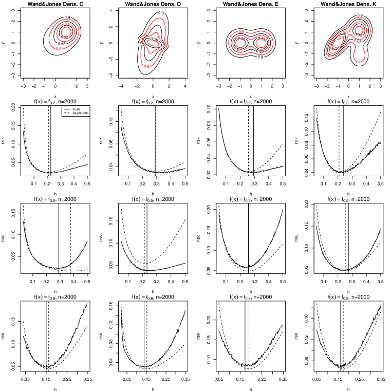
Figure 2: Comparison of the simulated true risk function $\mathbb{E}[\mu_{f_{0}}\{\mathcal{L}(c)\Delta\widehat{\mathcal{L}}_{\boldsymbol{H}}(c)\}]$ with $\text{LS}(\boldsymbol{H})$ for four densities in Wand and Jones (1993). The panels in the first row are the contour plots for four densities with the contours of interest plotted in red color. The panels in the rest of the rows are the comparison plots for the simulated true risk (solid line) and $\text{LS}(\boldsymbol{H})$ (dashed line) corresponding to the density at the top of the column for $\tau=0.2,0.5,0.8$. The positions of the solid vertical line and the dashed line stand for the optimal bandwidths obtained from the simulated true risk and the asymptotic approximation respectively over the restricted class $\mathcal{S}_{1}$. The sample size for all the cases is 2000.

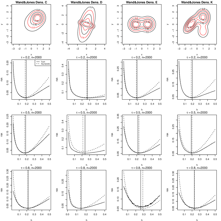
Figure 3: Comparison of the simulated true risk function $\mathbb{E}[\mu_{f_{0}}\{\mathcal{L}_{\tau}\Delta\widehat{\mathcal{L}}_{\tau,\boldsymbol{H}}\}]$ with $\text{HDR}(\boldsymbol{H})$ for four densities in Wand and Jones (1993). The panels in the first row are the contour plots for four densities with the contours of interest plotted in red color. The panels in the rest of the rows are the comparison plots for the simulated true risk (solid line) and the $\text{HDR}(\boldsymbol{H})$ (dashed line) corresponding to the density at the top of column for $\tau=0.2,0.5,0.8$. The positions of the solid vertical line and the dashed line stand for the optimal bandwidths obtained from the simulated true risk and the asymptotic approximation respectively over the restricted class $\mathcal{S}_{1}$. The sample size for all the cases is 2000.

We ran a simulation study to compare the performance of our bandwidth selection method with LSCV for all the 12 densities in Wand and Jones (1993) and for density (11). For each density function, 250 Monte Carlo samples with 2000 observations were generated. For each sample, we estimated the 0.2, 0.5, 0.8 HDR with bandwidth matrices chosen by our method and LSCV respectively. The HDR error $\mu_{f_{0}}\{\mathcal{L}_{\tau}\Delta\widehat{\mathcal{L}}_{\tau,\boldsymbol{H}}\}$ was calculated for each method in each replication. Figure 4 shows the plot of the estimation errors generated by the two methods for density (11). Figure 5 shows the boundaries of the estimated HDR by HDR bandwidth and by the LSCV bandwidth selector from one of the simulated samples. We can see for $\tau=0.2,0.5$, the performance of HDR bandwidth selector outperformed LSCV bandwidth selector greatly for each simulated instance. For $\tau=0.8$, the HDR bandwidth performed slightly less well than the LSCV bandwidth on average. One hypothesis for why our method suffers when $\tau=.8$ is that Assumption Assumption D1b requires that $\|\nabla f_{0}\|>0$ in a neighborhood of the HDR. However, when $\tau=.8$, $f_{0}$ is close to having gradient zero on the true HDR which is close to the density mode.

Figure 4: Plot of simulated errors generated by HDR-tailored bandwidth and LSCV for the sharp mode density (11). The horizontal axis stands for errors of HDR bandwidth and vertical axis stands for errors of LSCV bandwidth.

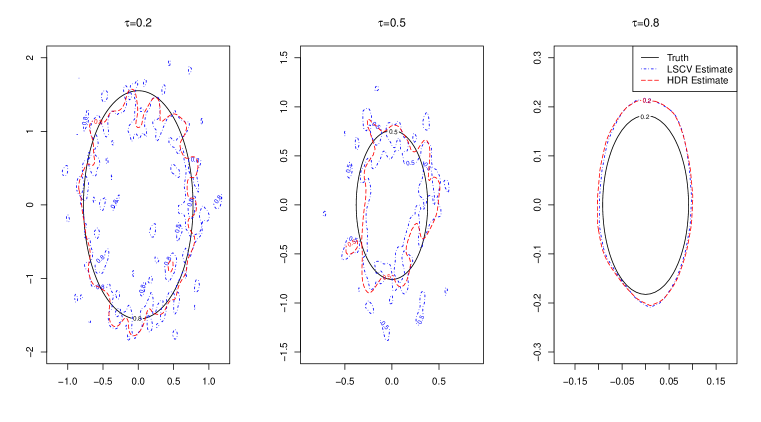
Figure 5: Plot of boundaries of true HDR, HDR estimated by HDR bandwidth and HDR estimated by LSCV bandwidth from one simulated sample with 2000 observations. The three panels correspond to $\tau=0.2,0.5,0.8$ respectively.

It is worth noticing in Figure 5 that the HDR estimated by our method discovers the true underlying topological structure of the density, while the HDR estimated by LSCV does a very poor job of revealing the topological structure when $\tau=.2$ or $.5$ (the LSCV estimates have many spurious separate connected components rather than a single one).

Applying the Wilcoxon signed rank test to the simulated paired errors genererated by our HDR bandwidth and LSCV bandwidth showed that for $\tau=0.2$, our method outperformed LSCV for 12 out of 13 density functions; for $\tau=0.5$, our method did better for 8 out of 13 density functions; for $\tau=0.8$, our method did better in 8 out of 13 density functions.

Note that for any given fixed density, it is likely to be the case for some HDR that the MISE-optimal bandwidth and the HDR-optimal bandwidth will approximately coincide. Thus we may not expect our method to be better than LSCV for all densities and levels simultaneously. Of course, in practice one does not know whether LSCV will work well for the $\tau$ value one is interested in. Our HDR method appears to work well for lower $\tau$ values, which are the useful values in many applications of HDR estimation. For example in novelty detection, the value of $\tau$ equals the probability of type-I error which is often set to be $0.05$ or $0.1$; in clustering analysis, $\tau$ corresponds to fraction of the data that will be discarded during analysis and is also set to be a value close to $0$. As mentioned in the previous paragraph, this may be related to the assumption that $\|\nabla f_{0}\|>0$ on the HDR boundary. Relaxing this assumption is an important direction for future work, but seems likely to involve somewhat different approximations than the ones used in this paper.

	$\tau=0.2$		$\tau=0.5$		$\tau=0.8$
Density	Test statistic	p-value	Test statistic	p-value	Test statistic	p-value
Density A	27743	¡2.2e-16	25356	1.816e-14	26608	¡2.2e-16
Density B	27743	¡2.2e-16	25297	¡2.2e-16	26361	¡2.2e-16
Density C	23200	¡2.2e-16	25419	¡2.2e-16	20725	5.388e-06
Density D	31349	¡2.2e-16	29159	¡2.2e-16	799	1
Density E	28630	¡2.2.e-16	22430	1.923e-09	24220	4.503e-14
Density F	24756	1.159e-15	3223	1	6433	1
Density G	29997	¡2.2e-16	14861	0.765	16265	0.3071
Density H	25968	¡2.2e-16	11889	0.9996	10535	1
Density I	8419	1	3713	1	3643	1
Density J	29488	¡2.2e-16	18411	0.008676	28905	¡2.2e-16
Density K	24555	4.689e-15	21411	2.861e-07	19746	0.0001958
Density L	24658	2.3e-15	15659	0.5101	18997	0.001919

Table 1: Summary of Wilcoxon tests for the errors generatated by LSCV bandwidth and HDR bandwidth. The alternative hypothesis is the errors generated by LSCV bandwidth are large. Tests were done for 250 errors simulated from each of the 12 densities in Wand and Jones (1993) at $\tau=0.2,0.5,0.8$. Test statistics and the corresponding p-values are summarized in the table. Use $\widehat{f}_{n,\boldsymbol{H}_{0}}$ to estimate $\beta_{\tau}$

	$\tau=0.5$		$\tau=0.2$		$\tau=0.8$
Density	Test statistic	p-value	Test statistic	p-value	Test statistic	p-value
Density A	25385	¡2.2e-16	29238	¡2.2e-16	26520	¡2.2e-16
Density B	25690	¡2.2e-16	29290	¡2.2e-16	23990	2.027e-13
Density C	27574	¡2.2e-16	24585	3.814e-15	21568	1.392e-07
Density D	29298	¡2.2e-16	31363	¡2.2e-16	1486	1
Density E	21824	4.133e-08	29934	2.2e-16	22241	5.154e-09
Density F	5344	1	25023	¡2.2e-16	9866	1
Density G	15348	0.6168	28737	¡2.2e-16	17723	0.0377
Density H	16244	0.3136	25987	¡2.2e-16	11732	1
Density I	4573	1	9796	1	4485	1
Density J	20982	¡1.868e-06	29863	¡2.2e-16	29830	¡2.2e-16
Density K	21595	1.227e-07	21842	3.788e-08	22701	4.463e-10
Density L	16854	0.1542	24077	1.153e-13	20861	3.094e-06

Table 2: Summary of Wilcoxon tests for the errors generatated by LSCV bandwidth and HDR bandwidth. The alternative hypothesis is the errors generated by LSCV bandwidth are large. Tests were done for 250 errors simulated from each of the 12 densities in Wand and Jones (1993) at $\tau=0.2,0.5,0.8$. Test statistics and the corresponding p-values are summarized in the table. Use $\widehat{f}_{n,\boldsymbol{H}_{1}}$ to estimate $\beta_{\tau}$

4.2 Real data analysis

We now discuss two real datasets. The Wisconsin Diagnostic Breast Cancer data contains 699 instances of breast cancer cases with 458 of them being benign instances and 241 being malignant instances. Nine cancer-related features were measured for each instance. For the Banknote Authentication data, images were taken of 1372 banknotes, some fake and some genuine. Wavelet transformation tools were used to extract four descriptive features of the images. For both datasets, we reduced the original features to the first two principal components. We apply our method to perform novelty detection for the two data sets. Novelty detection is like a classification problem where only the “normal” class is observed in the training data. Then, for a new data point $\boldsymbol{x}_{\text{new}}$, we want to test the null hypothesis $H_{0}:\boldsymbol{x}_{\text{new}}\text{ is a normal point}$ (or, alternatively, to classify $\boldsymbol{x}_{\text{new}}$ as “normal” or “anomalous”). For level set (HDR) based novelty detection, we can consider an oracle decision rule, or acceptance region, $A:=\{\boldsymbol{x}:f_{0}(\boldsymbol{x})\geq c\}$ (based on knowing $f_{0}$); if $f_{0}(\boldsymbol{x}_{\text{new}})\in A$, we accept the null hypothesis, and we reject otherwise. For the breast cancer data, “normal” means healthy, and for the banknote data, “normal” means genuine. If we take $c=f_{\tau}$, then the oracle decision rule will have type-I error, or False Positive Rate (FPR), of $\tau$ (under a regularity condition). Additionally, under regularity conditions, $A$ has the minimum volume of any acceptance rule with FPR of $\tau$, since HDR’s are minimum volume sets (Garcia et al., 2003). This property is beneficial for controlling the type-II error rate, or False Negative Rate (although the actual False Negative Rate depends on the unknown “anomaly” distribution).

In this section, for each of the two data sets we use a KDE with our bandwidth selection procedure to estimate an HDR based on the “normal” class data and use the estimated HDR to perform classification. We delete the observations with missing values for any covariates and randomly split the data set into two parts, training data and testing data. For the Wisconsin Breast Cancer data, 345 benign instances are contained in the training data and 200 (with half being benign and another half being malignant) are contained in the testing data. For the Banknote Authentication data, 400 genuine instances are contained in the training data and again, 200 (with half being genuine and another half being fake) are contained in the testing data. We estimate the $90\%$ HDR using our method based on the training data. The first row of Figure 6 shows the plot of the data and the boundaries of the $90\%$ HDR which are the decision boundaries for the two classification problems. The asymptotic FPR in these two classification problems is $\tau=0.1$. For the Wisconsin Breast Cancer data, on the test data, the observed FPR is $0.09$ and the True Positive Rate (TPR) is $0.99$. For the Banknote Authentication data, the observed FPR is $0.04$, and the observed TPR is $0.61$. We also generated full ROC curves for the two datasets which are shown in the second row of Figure 6. The ROC curves are based on $30$ different splits of the data into training and test sets (with the reported FPR and TPR given by the averages over the 30 test sets). The ROC curve clearly shows that the Wisconsin Breast Cancer data is an example where HDR-based anomaly detection is highly effective. The Banknote data is not as easy for our method; it may be the case that using an HDR based on all four variables improves the classification performance. We leave the very interesting question of how best to combine HDR-based classification with dimension reduction for future work.

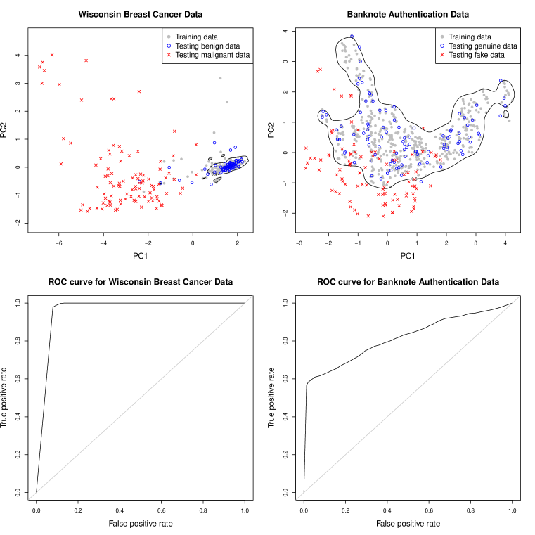
Figure 6: Plot of data and boundary of estimated $90\%$ HDR for the Wisconsin Diagnostic Breast Cancer Data and Banknote Authentication Data. Solid dots correspond to training data, circles are testing data of normal instances and crosses are testing data of anomaly instances. The two panels in the second row are the corresponding ROC curves for the two classification problems.

5 Discussion

In this paper, we derive asymptotic expansions of the symmetric risk for LS estimation and HDR estimation based on kernel density estimators. We provide an efficient bandwidth selection procedure using a plug-in strategy. We also study by theory and by simulation the performance of our bandwidth selector. Simulation studies show that both our asymptotic expansion and our bandwidth selector are effective tools. The two asymptotic risk approximations we provide may also be useful in the analysis of other procedures, developed in future work, for doing LS or HDR bandwidth selection.

As discussed in the Introduction, the interesting paper Qiao (2018) also considers problems of bandwidth selection for KDE’s via minimizing asymptotic expansions of risk functions that are based on loss functions related to level sets. Qiao (2018) does not consider HDR estimation. Qiao (2018) does consider the LS estimation problem. Our Theorem 2.1 is similar to Qiao (2018)’s Corollary 3.1; both results consider the LS estimation setting, and give risk expansions based on loss functions that are given by integrating the symmetric set differences against $f_{0}$ (or against something similar). Our theorem requires only that $f_{0}$ have two continuous derivatives in a neighborhood of $\beta(c)$ (which we believe to be approximately the weakest possible conditions), whereas Qiao (2018) requires four continuous derivatives. On the other hand, Qiao (2018) allows for using higher order kernels if one has higher order smoothness of $f_{0}$. While Qiao (2018)’s Corollary 3.1 studies the same risk function approximation, $\operatorname{LS}(\cdot)$, that we study in our Theorem 2.1, Qiao (2018) does not present any algorithm for minimizing $\operatorname{LS}(\cdot)$ and thus presents no simulations related to $\operatorname{LS}(\cdot)$. Rather, Qiao (2018) focuses more attention on a different risk function (the “excess risk”) approximation that allows for an analytic solution, at least when $d=2$.

There are many interesting avenues for extending the work done in the present paper. We describe a few here.

1. (Regression and classification) In the present paper we have considered only the density estimation context, but estimation of level sets of regression functions estimated by kernel-based methods is also interesting, as is consideration of classification problems.

   Regression level set estimation has received less attention than density level set estimation, although it has been studied in some settings; Cavalier (1997) studies multivariate nonparametric regression level set minimax rates of convergence.

   One method for classification is to estimate densities for different classes and then classify a point by the class density having highest value at the point. In that case, rather than estimating a level set of one density, one is estimating the $0$ level set of a difference of two densities. Mason and Polonik (2009, page 1110) discuss this approach to classification. In the context of an application in flow cytometry, Duong et al. (2009) also study estimation of HDR’s of density differences (without specifically focusing on classification). We believe the methods of this paper can be extended to those contexts.

2. (Topological data analysis and critical points) Another important avenue of research is to consider modifications of the assumptions under which our approximations hold. Level set estimation is one of the main tools in topological data analysis (TDA). Estimation of LS’s which have zero gradient (at some points) on the boundary (which is ruled out by our assumptions) is of great interest in TDA, because the topology of level sets can change as the level crosses critical points (points having zero gradient). In fact, in the context of using tools based on level set estimates, Wasserman (2016, Section 5) states that “the problem of choosing tuning parameters is one of the biggest open challenges in TDA”. Thus, developing tools for bandwidth selection when the gradient is zero would be very useful for TDA. Unfortunately, at points where the gradient is zero we cannot apply the inverse function theorem which is used in Lemma A.1 (implicitly) and by several results in Appendix B, so a very different analysis than the one we completed here may be necessary in such cases. In general, there are very few theoretical works on level set estimation at levels that contain critical values (points where $\nabla f_{0}$ is $0$). In fact, the only one we know of is Chen (2016), in which a rate of convergence of $\lambda\left\{\mathcal{L}(c)\Delta\widehat{\mathcal{L}}_{\boldsymbol{H}}(c)\right\}$ (where $\lambda$ is Lebesgue measure) is derived.

3. (MCMC level sets) The work in this paper is restricted to the case where $\boldsymbol{X}_{1},\ldots,\boldsymbol{X}_{n}$ are independent. An important extension is to allow the $\boldsymbol{X}_{i}$ to be samples from a Markov chain. It is well known that KDE’s often work similarly when the data exhibit weak dependence as when they are independent (Wand and Jones, 1995). This would allow our tools for HDR estimation to be used to form credible regions based on Markov chain Monte Carlo output in Bayesian statistical analyses. At present, ad-hoc methods are often used for forming credible regions based on Markov chain Monte Carlo output.

Appendix A Proof of main results

A.1 Proof of Theorem 2.2

First, we observe that

$$\mu_{f_{0}}(\mathcal{L}_{\tau}\Delta\hat{\mathcal{L}}_{\tau,\boldsymbol{H}}) =\int_{\mathbb{R}^{d}}f_{0}(\boldsymbol{x})\left|\mathbbm{1}_{\left\{\widehat{f}_{n,\boldsymbol{H}}(\boldsymbol{x})\geq\widehat{f}_{\tau,n}\right\}}-\mathbbm{1}_{\left\{f_{0}(\boldsymbol{x})\geq f_{\tau,0}\right\}}\right|\,d\boldsymbol{x}$$

$$=\int_{\mathcal{L}_{\tau}^{c}}f_{0}(\boldsymbol{x})\mathbbm{1}_{\left\{\widehat{f}_{n,\boldsymbol{H}}(\boldsymbol{x})\geq\widehat{f}_{\tau,n}\right\}}\,d\boldsymbol{x}+\int_{\mathcal{L}_{\tau}}f_{0}(\boldsymbol{x})\mathbbm{1}_{\left\{\widehat{f}_{n,\boldsymbol{H}}(\boldsymbol{x})<\widehat{f}_{\tau,n}\right\}}\,d\boldsymbol{x}.$$

Then by Tonelli’s Theorem (Folland, 1999, Theorem 2.37), we have

$$\begin{split}\mathbb{E}\left[\mu_{f_{0}}\{\mathcal{L}_{\tau}\Delta\widehat{\mathcal{L}}_{\tau,\boldsymbol{H}}\}\right]&=\int_{\mathcal{L}_{\tau}^{c}}f_{0}(\boldsymbol{x})P\left(\widehat{f}_{n,\boldsymbol{H}}(\boldsymbol{x})\geq\widehat{f}_{\tau,n}\right)\,d\boldsymbol{x}\\ &\quad+\int_{\mathcal{L}_{\tau}}f_{0}(\boldsymbol{x})P\left(\widehat{f}_{n,\boldsymbol{H}}(\boldsymbol{x})<\widehat{f}_{\tau,n}\right)\,d\boldsymbol{x}.\end{split}$$ (12)

For a density function $f$ on $\mathbb{R}^{d}$, let $f_{\tau}(f):=\inf\{\boldsymbol{y}\geq 0:\int_{\mathbb{R}^{d}}f(\boldsymbol{x})\mathbbm{1}_{\{f(\boldsymbol{x})\geq\boldsymbol{y}\}}\,d\boldsymbol{x}\leq 1-\tau\}$. By this definition, $f_{\tau,0}\equiv f_{\tau}(f_{0})$. The following lemma bounds the modulus of continuity of $f_{\tau}$ when the difference between two density functions is sufficiently small.

Lemma A.1.

Let the assumptions of Theorem 2.2 hold. Let $\tilde{f}$ be another uniformly continuous density function on $\mathbb{R}^{d}$ and $\tilde{f}_{\tau}\equiv f_{\tau}(\tilde{f})$. Then there exists a constant $C_{1}\geq 1$ such that for all $\varepsilon>0$ sufficiently small, $|\tilde{f}_{\tau}-f_{\tau,0}|\leq C_{1}\varepsilon$ whenever $\|\tilde{f}-f_{0}\|_{\infty}\leq\varepsilon$.

It is intuitively believable that when the sample size $n$ is sufficiently large, the values of the two integrals on the right of (12) are mostly governed by the integrals over a small neighborhood of $\beta_{\tau}$. To shrink the region of integration, for $\delta>0$, and for a given level $t>0$, we let $\beta^{\delta}(t):=\bigcup_{\boldsymbol{x}\in\beta(t)}B(\boldsymbol{x},\delta)$, and $\beta^{\delta}_{\tau}\equiv\beta^{\delta}(f_{\tau,0})$. We also let

$$\mathcal{L}_{\delta}(f_{\tau,0}):=\bigcup_{\boldsymbol{x}\in\mathcal{L}_{\tau}}B(\boldsymbol{x},\delta)\quad\text{and}\quad\mathcal{L}_{-\delta}(f_{\tau,0}):=\mathcal{L}(f_{\tau,0})\backslash\beta_{\tau}^{\delta}.$$

Then we can shrink the integral region using the following lemma.

Lemma A.2.

Let the assumptions of Theorem 2.2 hold. Then for a sequence $\delta_{n}>0$ converging to 0 such that $\lambda_{\max}(\boldsymbol{H})=o(\delta_{n})$, we will have

$$\int_{\mathcal{L}_{\delta_{n}}(f_{\tau,0})^{c}}f_{0}(\boldsymbol{x})P\left(\widehat{f}_{n,\boldsymbol{H}}(\boldsymbol{x})\geq\widehat{f}_{\tau,n}\right)\,d\boldsymbol{x}+\int_{\mathcal{L}_{-\delta_{n}}(f_{\tau,0})}f_{0}(\boldsymbol{x})P\left(\widehat{f}_{n,\boldsymbol{H}}(\boldsymbol{x})<\widehat{f}_{\tau,n}\right)\,d\boldsymbol{x}$$ (13)

is $o(n^{-1})$ as $n\rightarrow\infty$.

The definition of $\widehat{f}_{\tau,n}$ is simple and straightforward, however there is no explicit form for this quantity. So we want to seek an asymptotic expansion for $\widehat{f}_{\tau,n}$. For a uniformly continuous density $f$ on $\mathbb{R}^{d}$ and $y\geq 0$, we define

$$\psi(f,y):=\int_{\mathbb{R}^{d}}f(\boldsymbol{x})\mathbbm{1}_{\{f(\boldsymbol{x})\geq y\}}\,d\boldsymbol{x}.$$

First, we observe for $\varepsilon>0$ sufficiently small,

$$\begin{split}&\left|\psi(f_{0},f_{\tau,0}+\varepsilon)-\psi(f_{0},f_{\tau,0})-\varepsilon\int_{\beta_{\tau}}\frac{f_{0}(\boldsymbol{x})}{\|\nabla f_{0}(\boldsymbol{x})\|}\,d\mathcal{H}(\boldsymbol{x})\right|\\ &=\left|\int_{\mathbb{R}^{d}}f_{0}(\boldsymbol{x})\mathbbm{1}_{\{f_{\tau,0}\leq f_{0}(\boldsymbol{x})\leq f_{\tau,0}+\varepsilon\}}\,d\boldsymbol{x}-\varepsilon\int_{\beta_{\tau}}\frac{f_{0}(\boldsymbol{x})}{\|\nabla f_{0}(\boldsymbol{x})\|}\,d\mathcal{H}(\boldsymbol{x})\right|=O(\varepsilon^{2}),\end{split}$$ (14)

as $\varepsilon\searrow 0$, where the last line comes from a similar argument of (71) and (72). A similar argument shows the same result when $\varepsilon\nearrow 0$. Next, we look at

$$\begin{split}&\left|\psi(\tilde{f},\tilde{f}_{\tau})-\psi(f_{0},\tilde{f}_{\tau})-f_{\tau,0}\int_{\beta_{\tau}}\frac{g}{\|\nabla f_{0}\|}\,d\mathcal{H}-\int_{\mathcal{L}_{\tau}}g\,d\lambda\right|\\ &=\left|\int\tilde{f}\mathbbm{1}_{\{\tilde{f}\geq\tilde{f}_{\tau}\}}\,d\lambda-\int f_{0}\mathbbm{1}_{\{f_{0}\geq\tilde{f}_{\tau}\}}\,d\lambda-f_{\tau,0}\int_{\beta_{\tau}}\frac{g}{\|\nabla f_{0}\|}\,d\mathcal{H}-\int_{\mathcal{L}_{\tau}}g\,d\lambda\right|\\ &=\left|\int f_{0}(\mathbbm{1}_{\{\tilde{f}\geq\tilde{f}_{\tau}\}}-\mathbbm{1}_{\{f_{0}\geq\tilde{f}_{\tau}\}})\,d\lambda-f_{\tau,0}\int_{\beta_{\tau}}\frac{g}{\|\nabla f_{0}\|}\,d\mathcal{H}\right.\\ &\qquad+\left.\int g(\mathbbm{1}_{\{\tilde{f}\geq\tilde{f}_{\tau}\}}-\mathbbm{1}_{\{f_{0}\geq f_{\tau,0}\}})\,d\lambda\right|,\end{split}$$ (15)

where $g(\boldsymbol{x})=\tilde{f}(\boldsymbol{x})-f_{0}(\boldsymbol{x})$. For the first integral on the last line, since $\mathbbm{1}_{\{\tilde{f}\geq\tilde{f}_{\tau}\}}-\mathbbm{1}_{\{f_{0}\geq\tilde{f}_{\tau}\}}\neq 0$ indicates that $\tilde{f}(\boldsymbol{x})\geq\tilde{f}_{\tau},f_{0}(\boldsymbol{x})<\tilde{f}_{\tau}$ or $\tilde{f}(\boldsymbol{x})<\tilde{f}_{\tau},f_{0}(\boldsymbol{x})\geq\tilde{f}_{\tau}$, we have $f_{0}(\boldsymbol{x})\in[\tilde{f}_{\tau}-|g(\boldsymbol{x})|,\tilde{f}_{\tau}+|g(\boldsymbol{x})|]$. Combining (16) with our result in Lemma A.1 yields

$$f_{0}(\boldsymbol{x})=f_{\tau}+O(\|g\|_{\infty}),$$ (16)

for $\boldsymbol{x}\in\{\boldsymbol{y}:\tilde{f}(\boldsymbol{y})\geq\tilde{f}_{\tau}\}\Delta\{\boldsymbol{y}:f_{0}(\boldsymbol{y})\geq\tilde{f}_{\tau}\}$. Next we need the following lemmas.

Lemma A.3.

Let the assumptions of Theorem 2.2 hold and the notation be as defined above. As $\|g\|_{\infty}^{2}+\|g\|_{\infty}\|\nabla g\|_{\infty}\to 0$, we have

$$\int\mathbbm{1}_{\{\tilde{f}\geq\tilde{f}_{\tau}\}}-\mathbbm{1}_{\{f_{0}\geq\tilde{f}_{\tau}\}}\,d\lambda=\int_{\beta_{\tau}}\frac{g}{\|\nabla f_{0}\|}\,d\mathcal{H}+O(\|g\|_{\infty}^{2}+\|g\|_{\infty}\|\nabla g\|_{\infty}).$$ (17)

Lemma A.4.

Let the assumptions of Theorem 2.2 hold and the notation be as defined above. As $\|g\|^{2}_{\infty}+\|g\|_{\infty}\|\nabla g\|_{\infty}\rightarrow 0$, we have

$$\int_{\mathbb{R}^{d}}g(\boldsymbol{x})\left(\mathbbm{1}_{\{\tilde{f}(\boldsymbol{x})\geq\tilde{f}_{\tau}\}}-\mathbbm{1}_{\{f_{0}(\boldsymbol{x})\geq f_{\tau}\}}\right)\,d\boldsymbol{x}=O(\|g\|^{2}_{\infty}).$$

Now with Lemma A.3, A.4 and (16), we see that (15) equals $O(\|g\|_{\infty}^{2}+\|g\|_{\infty}\|\nabla g\|_{\infty})$. Because

$$\left|\psi(\tilde{f},\tilde{f}_{\tau})-\psi(f_{0},\tilde{f}_{\tau})-f_{\tau,0}\int_{\beta_{\tau}}\frac{g}{\|\nabla f_{0}\|}\,d\mathcal{H}-\int_{\mathcal{L}_{\tau}}g\,d\lambda\right|$$

$$=\left|\int f(\mathbbm{1}_{\{\tilde{f}\geq\tilde{f}_{\tau}\}}-\mathbbm{1}_{\{f\geq\tilde{f}_{\tau}\}})\,d\boldsymbol{x}-f_{\tau,0}\int_{\beta_{\tau}}\frac{g}{\|\nabla f_{0}\|}\,d\mathcal{H}+\int g(\mathbbm{1}_{\{\tilde{f}\geq\tilde{f}_{\tau}\}}-\mathbbm{1}_{\{f\geq f_{\tau}\}})\,d\boldsymbol{x}\right|$$

$$=\left|(f_{\tau,0}+O(\|g\|_{\infty})\left(\int_{\beta_{\tau}}\frac{g}{\|\nabla f_{0}\|}\,d\mathcal{H}+O(\|g\|_{\infty}^{2}+\|g\|_{\infty}\|\nabla g\|_{\infty})\right)\right.$$

$$\qquad\left.-f_{\tau,0}\int_{\beta_{\tau}}\frac{g}{\|\nabla f_{0}\|}\,d\mathcal{H}+O(\|g\|_{\infty}^{2}+\|g\|_{\infty}\|\nabla g\|_{\infty})\right|$$

$$=O(\|g\|_{\infty}^{2}+\|g\|_{\infty}\|\nabla g\|_{\infty}).$$

Note that if $\|\nabla g\|_{\infty}\rightarrow 0$, then $\psi(\tilde{f},\tilde{f}_{\tau})=1-\tau$. Combining this with (14) and the order of (15), we have

$$\begin{split}0&=\psi(\tilde{f},\tilde{f}_{\tau})-\psi(f,f_{\tau,0})\\ &=\psi(\tilde{f},\tilde{f}_{\tau})-\psi(f,\tilde{f}_{\tau})+\psi(f,\tilde{f}_{\tau})-\psi(f,f_{\tau,0})\\ &=-(\tilde{f}_{\tau}-f_{\tau,0})f_{\tau,0}\int_{\beta_{\tau}}\frac{1}{\|\nabla f_{0}\|}\,d\mathcal{H}+f_{\tau,0}\int_{\beta_{\tau}}\frac{g}{\|\nabla f_{0}\|}\,d\mathcal{H}\\ &\qquad+\int_{\mathcal{L}_{\tau}}g\,d\boldsymbol{x}+O(\|g\|_{\infty}^{2}+\|g\|_{\infty}\|\nabla g\|_{\infty})\end{split}$$ (18)

as $\|g\|_{\infty}^{2}+\|g\|_{\infty}\|\nabla g\|_{\infty}\rightarrow 0$. We want to apply (18) with $\tilde{f}=\widehat{f}_{n,\boldsymbol{H}}$, so that $g=\widehat{f}_{n,\boldsymbol{H}}-f_{0}$. To do this, note by Theorem B.1 (and so Assumptions Assumption H (as well as Assumptions LABEL:assm:DA and Assumption K)) that $\|\widehat{f}_{n,\boldsymbol{H}}-\mathbb{E}\widehat{f}_{n,\boldsymbol{H}}\|_{\infty}=O_{\text{a.s.}}\left(\sqrt{\frac{\log|\boldsymbol{H}|^{-1/2}}{n|\boldsymbol{H}|^{1/2}}}\right)$, $\|\nabla\widehat{f}_{n,\boldsymbol{H}}-\mathbb{E}\nabla\widehat{f}_{n,\boldsymbol{H}}\|_{\infty}=O_{a.s.}\left(\sqrt{\frac{\log|\boldsymbol{H}|^{-1/2}}{n|\boldsymbol{H}|^{1/2}\lambda_{\min}(\boldsymbol{H})}}\right)$, by (75), $\|\mathbb{E}(\widehat{f}_{n,\boldsymbol{H}})-f_{0}\|_{\infty}=O\left\{\lambda_{\max}(\boldsymbol{H})\right\}$. We also have $\|\mathbb{E}\nabla\widehat{f}_{n,\boldsymbol{H}}-\nabla f_{0}\|_{\infty}=O\{\lambda^{1/2}_{\max}(\boldsymbol{H})\}$. Because,

$$\mathbb{E}\nabla\widehat{f}_{n,\boldsymbol{H}}(\boldsymbol{x})=\mathbb{E}\nabla K_{\boldsymbol{H}}(\boldsymbol{x}-X_{1})=\nabla K_{H}\ast f_{0}(\boldsymbol{x})=K_{\boldsymbol{H}}*\nabla f_{0}(\boldsymbol{x}),$$

where $f\ast g(\boldsymbol{x})=\int_{\mathbb{R}^{d}}f(\boldsymbol{x}-\boldsymbol{y})g(\boldsymbol{y})\,d\boldsymbol{y}$ and $K_{\boldsymbol{H}}(\boldsymbol{x})=|\boldsymbol{H}|^{-1/2}K(\boldsymbol{H}^{-1/2}\boldsymbol{x})$. So

$$\mathbb{E}\nabla\widehat{f}_{n,\boldsymbol{H}}(\boldsymbol{x}) =\int_{\mathbb{R}^{d}}K_{\boldsymbol{H}}(\boldsymbol{x}-\boldsymbol{y})\nabla f_{0}(\boldsymbol{y})\,d\boldsymbol{y}$$

$$=\int_{\mathbb{R}^{d}}K(\boldsymbol{y})\nabla f_{0}(\boldsymbol{x}-\boldsymbol{H}^{1/2}\boldsymbol{y})\,d\boldsymbol{y}.$$

By Taylor Expansion, $\nabla f_{0}(\boldsymbol{x}-\boldsymbol{H}^{1/2}\boldsymbol{y})=\nabla f_{0}(\boldsymbol{x})-\nabla^{2}f_{0}(x-s_{\boldsymbol{y}}\boldsymbol{H}^{1/2}\boldsymbol{y})\boldsymbol{H}^{1/2}\boldsymbol{y}$, $s_{\boldsymbol{y}}\in(0,1)$ depends on $\boldsymbol{y}$. Now we have

$$\mathbb{E}\nabla\widehat{f}_{n,\boldsymbol{H}}(\boldsymbol{x}) =\nabla f_{0}(\boldsymbol{x})-\int_{\mathbb{R}^{d}}K(\boldsymbol{y})\nabla^{2}f_{0}(\boldsymbol{x}-s_{\boldsymbol{y}}\boldsymbol{H}^{1/2}\boldsymbol{y})H^{1/2}\boldsymbol{y}\,d\boldsymbol{y}.$$

By assumption LABEL:assm:DA $\nabla^{2}f_{0}$ is bounded, there exists $A\in\mathbb{R}^{d}$, such that

$$\left|\int_{\mathbb{R}^{d}}K(\boldsymbol{y})\nabla^{2}f_{0}(\boldsymbol{x}-s_{\boldsymbol{y}}\boldsymbol{H}^{1/2}\boldsymbol{y})H^{1/2}\boldsymbol{y}\,d\boldsymbol{y}\right|\leq H^{1/2}A.$$

Then applying the above results, we have

$$\begin{split}\widehat{f}_{\tau,n}-f_{\tau,0}&=w_{0}\left\{\int_{\beta_{\tau}}\frac{\widehat{f}_{n,\boldsymbol{H}}(\boldsymbol{x})-f_{0}(\boldsymbol{x})}{\|\nabla f_{0}(\boldsymbol{x})\|}\,d\mathcal{H}(\boldsymbol{x})+\frac{1}{f_{\tau,0}}\int_{\mathcal{L}_{\tau}}\widehat{f}_{n,\boldsymbol{H}}(\boldsymbol{x})-f_{0}(\boldsymbol{x})\,d\boldsymbol{x}\right\}\\ &\qquad+O_{p}\left(\frac{\log|\boldsymbol{H}|^{-1/2}}{n|\boldsymbol{H}|^{1/2}\sqrt{\lambda_{\max}(\boldsymbol{H})}}+\lambda_{\max}^{3/2}(\boldsymbol{H})\right).\end{split}$$ (19)

Note from (2) and (19), for fixed $\boldsymbol{x}$, $\widehat{f}_{n,\boldsymbol{H}}(\boldsymbol{x})-\widehat{f}_{\tau,n}$ can be expressed as the average of i.i.d. random variables with a negligible stochastic error term. This motivates us to use the Berry-Essen Theorem (Ferguson, 1996) to approximate the two probabilities appearing on the right of (13). In order to do so, we will need to approximate the mean and variance of $\widehat{f}_{\tau,n}$, which we do in the next lemmas.

Lemma A.5.

Let the assumptions of Theorem 2.2 hold and the notation be as defined above. Then we have

$$\begin{split}\mathbb{E}\widehat{f}_{\tau,n}-f_{\tau,0}&=w_{0}\left\{V_{1}(\boldsymbol{H})+V_{2}(\boldsymbol{H})\right\}+o\left\{\operatorname*{tr}(\boldsymbol{H})\right\},\end{split}$$ (20)

as $n\rightarrow\infty$.

Recall $V_{1}$ and $V_{2}$ are defined in Theorem 2.2. The next lemma shows $\operatorname*{Var}\widehat{f}_{\tau,n}$ is negligible compared with other terms in the expansion.

Lemma A.6.

Let the assumptions of Theorem 2.2 hold and the notation be as defined above. Then $\operatorname*{Var}\widehat{f}_{\tau,n}=o(n^{-1}|\boldsymbol{H}|^{-1/2})$.

Now according to Lemma A.2 and (12), we have

$$\mathbb{E}\mu_{f_{0}}(\mathcal{L}_{\tau}\Delta\hat{\mathcal{L}}_{\tau,\boldsymbol{H}}) =\int_{\mathcal{L}_{\tau}^{c}\backslash\mathcal{L}_{\delta_{n}}(f_{\tau})^{c}}f_{0}(\boldsymbol{x})P\left(\widehat{f}_{n,\boldsymbol{H}}(\boldsymbol{x})\geq\widehat{f}_{\tau,n}\right)\,d\boldsymbol{x}$$

$$\quad+\int_{\mathcal{L}_{\tau}\backslash\mathcal{L}_{-\delta_{n}}(f_{\tau,0})}f_{0}(\boldsymbol{x})P\left(\widehat{f}_{n,\boldsymbol{H}}(\boldsymbol{x})<\widehat{f}_{\tau,n}\right)\,d\boldsymbol{x}+o\left(n^{-1}\right)$$

$$=\int_{\beta_{\tau}^{\delta_{n}}}f_{0}(\boldsymbol{x})\left|P\left(\widehat{f}_{n,\boldsymbol{H}}(\boldsymbol{x})<\widehat{f}_{\tau,n}\right)\,d\boldsymbol{x}-\mathbbm{1}_{\{f_{0}(\boldsymbol{x})<f_{\tau,0}\}}\right|\,d\boldsymbol{x}+o\left(n^{-1}\right).$$

Then by Lemma B.4 when $\delta_{n}$ is small enough, the dominating term on the last line above is equal to

$$\begin{split}&\int_{\beta_{\tau}}\int_{-\delta_{n}}^{\delta_{n}}f_{0}(\boldsymbol{x}+tu_{\boldsymbol{x}})\left|P\left(\widehat{f}_{n,\boldsymbol{H}}(\boldsymbol{x}+tu_{\boldsymbol{x}})<\widehat{f}_{\tau,n}\right)-\mathbbm{1}_{\{f_{0}(\boldsymbol{x}+tu_{\boldsymbol{x}})<f_{\tau,0}\}}\right|\,dtd\mathcal{H}(\boldsymbol{x})\\ &\qquad+O(\delta_{n}^{2}),\end{split}$$ (21)

where $u_{\boldsymbol{x}}:=-\nabla f_{0}(\boldsymbol{x})/\|\nabla f_{0}(\boldsymbol{x})\|$ is the unit outer normal vector of $\beta_{\tau}$ at $\boldsymbol{x}$. Now for a fixed $\boldsymbol{x}\in\beta_{\tau}$, let $\boldsymbol{x}^{t}=\boldsymbol{x}+\frac{t}{\sqrt{n|\boldsymbol{H}|^{1/2}}}u_{\boldsymbol{x}}$ for $t\in[-\sqrt{n|\boldsymbol{H}|^{1/2}}\delta_{n},\sqrt{n|\boldsymbol{H}|^{1/2}}\delta_{n}]$, we see (21) equals

$$\frac{1}{\sqrt{n|\boldsymbol{H}|^{1/2}}}\int_{\beta_{\tau}}\int_{-\sqrt{n|\boldsymbol{H}|^{1/2}}\delta_{n}}^{\sqrt{n|\boldsymbol{H}|^{1/2}}\delta_{n}}f_{0}\left(\boldsymbol{x}^{t}\right)\left|P\left(\widehat{f}_{n,\boldsymbol{H}}\left(\boldsymbol{x}^{t}\right)<\widehat{f}_{\tau,n}\right)-\mathbbm{1}_{\{t>0\}}\right|\,dtd\mathcal{H}(\boldsymbol{x})$$ (22)

$$\qquad+O(\delta_{n}^{2}).$$ (23)

By Taylor Expansion, we have

$$f_{0}\left(\boldsymbol{x}+\frac{t}{\sqrt{n|\boldsymbol{H}|^{1/2}}}u_{\boldsymbol{x}}\right)=f_{0}(\boldsymbol{x})+\nabla f_{0}\left(\boldsymbol{x}+\frac{st}{\sqrt{n|\boldsymbol{H}|^{1/2}}}u_{\boldsymbol{x}}\right)^{\prime}\frac{t}{\sqrt{n|\boldsymbol{H}|^{1/2}}}u_{\boldsymbol{x}},$$

for some $s\in[0,1]$. Since by Assumption Assumption D1b, $f_{0}$ has bounded first derivatives, we see the dominating term in (22) equals

$$\begin{split}\frac{f_{\tau,0}}{\sqrt{n|\boldsymbol{H}|^{1/2}}}\int_{\beta_{\tau}}\int_{-\sqrt{n|\boldsymbol{H}|^{1/2}}\delta_{n}}^{\sqrt{n|\boldsymbol{H}|^{1/2}}\delta_{n}}\left|P\left(\widehat{f}_{n,\boldsymbol{H}}(\boldsymbol{x}^{t})<\widehat{f}_{\tau,n}\right)-\mathbbm{1}_{\{t>0\}}\right|\,dtd\mathcal{H}(\boldsymbol{x})+O(\delta_{n}^{2}),\end{split}$$ (24)

as $n\rightarrow\infty$. Because

$$\frac{1}{\sqrt{n|\boldsymbol{H}|^{1/2}}}\int_{\beta_{\tau}}\int_{-\sqrt{n|\boldsymbol{H}|^{1/2}}\delta_{n}}^{\sqrt{n|\boldsymbol{H}|^{1/2}}\delta_{n}}\frac{t}{\sqrt{n|\boldsymbol{H}|^{1/2}}}\,dt=O(\delta_{n}^{2}).$$

We can further shrink the region of interest by the following lemma.

Lemma A.7.

Let the assumptions of Theorem 2.2 hold and the notation be as defined above. Then for $n$ sufficiently large, $\mathbb{E}\{\widehat{f}_{n,\boldsymbol{H}}(\boldsymbol{x}^{t})-\widehat{f}_{\tau,n}\}$ is a strictly monotone function of $t\in[-\sqrt{n|\boldsymbol{H}|^{1/2}}\delta_{n},\sqrt{n|\boldsymbol{H}|^{1/2}}\delta_{n}]$, with a unique zero $t_{\boldsymbol{x}}^{\ast}$. For a sequence $t_{n}$ diverging to infinity and $t_{n}=O(\sqrt{n|\boldsymbol{H}|^{1/2}}\delta_{n})$, let

$$I_{\boldsymbol{x}}^{n}=[-\sqrt{n|\boldsymbol{H}|^{1/2}}\delta_{n},\sqrt{n|\boldsymbol{H}|^{1/2}}\delta_{n}]\backslash[t^{\ast}_{\boldsymbol{x}}-t_{n},t^{\ast}_{\boldsymbol{x}}+t_{n}].$$

We have

$$\int_{\beta_{\tau}}\int_{I_{\boldsymbol{x}}^{n}}|P(\widehat{f}_{n,\boldsymbol{H}}(\boldsymbol{x}^{t})<\widehat{f}_{\tau,n})-\mathbbm{1}_{\{t>0\}}|\,dtd\mathcal{H}(\boldsymbol{x})\rightarrow 0$$ (25)

as $n\rightarrow\infty$.

To complete the proof of Theorem 2.2, by (24) and Lemma A.7 it suffices to show that there exists a sequence $t_{n}$ diverging to infinity slowly such that

$$\frac{f_{\tau,0}}{\sqrt{n|\boldsymbol{H}|^{1/2}}}\int_{\beta_{\tau}}\int_{t^{\ast}_{\boldsymbol{x}}-t_{n}}^{t^{\ast}_{\boldsymbol{x}}+t_{n}}|P(\widehat{f}_{n,\boldsymbol{H}}(\boldsymbol{x}^{t})<\widehat{f}_{\tau,n})-\mathbbm{1}_{\{t<0\}}|\,dtd\mathcal{H}(\boldsymbol{x})$$

$$=\operatorname{HDR}(\boldsymbol{H})+o\left\{(n|\boldsymbol{H}|^{1/2})^{-1/2}+\operatorname*{tr}(\boldsymbol{H})\right\}.$$

For $i=1,2,\ldots,n$, let $Z_{ni}(\boldsymbol{x})=K_{\boldsymbol{H}}(\boldsymbol{x}-\boldsymbol{X}_{i})$ and $\bar{Y}_{n}=n^{-1}\sum_{i=1}^{n}Y_{ni}$, where

$$Y_{ni} =Z_{ni}(\boldsymbol{x}^{t})-f_{\tau,0}-\left\{\int_{\beta_{\tau}}\frac{1}{\|\nabla f_{0}\|}\,d\mathcal{H}\right\}^{-1}\left\{\int_{\beta_{\tau}}\frac{Z_{ni}(\boldsymbol{x})-f_{0}(\boldsymbol{x})}{\|\nabla f_{0}(\boldsymbol{x})\|}\,d\mathcal{H}(\boldsymbol{x})\right.$$

$$\qquad\left.+\frac{1}{f_{\tau,0}}\int_{\mathcal{L}_{\tau}}Z_{ni}(\boldsymbol{x})-f_{0}(\boldsymbol{x})\,d\boldsymbol{x}\right\}.$$

Then by (18) and (19), we can write $\widehat{f}_{n,\boldsymbol{H}}(\boldsymbol{x}^{t})-\widehat{f}_{\tau,n}=\bar{Y}_{n}+R_{n}$, where $R_{n}-\mathbb{E}(R_{n})=o_{p}\left(\frac{1}{\sqrt{n|\boldsymbol{H}|^{1/2}}}\right)$. Because by (18) we have

$$R_{n}=\left(\widehat{f}_{\tau,n}-f_{\tau,0}\right)\int_{\beta_{\tau}}\frac{1}{\|\nabla f_{0}\|}\,d\mathcal{H}-\int_{\beta_{\tau}}\frac{\widehat{f}_{n,\boldsymbol{H}}-f_{0}}{\|\nabla f_{0}\|}\,d\mathcal{H}-\frac{1}{f_{\tau,0}}\int_{\mathcal{L}_{\tau}}\left(\widehat{f}_{n,\boldsymbol{H}}-f_{0}\right)\,d\lambda,$$

and from Lemma A.6 we know $\operatorname*{Var}\widehat{f}_{\tau,n}=o(n^{-1}|\boldsymbol{H}|^{-1/2})$, $\operatorname*{Var}(\int_{\beta_{\tau}}\frac{\widehat{f}_{n,\boldsymbol{H}}-f_{0}}{\|\nabla f_{0}\|}\,d\mathcal{H})=o(n^{-1}|\boldsymbol{H}|^{-1/2})$ and $\operatorname*{Var}(\int_{\mathcal{L}_{\tau}}\left(\widehat{f}_{n,\boldsymbol{H}}-f_{0}\right)\,d\lambda=o(n^{-1}|\boldsymbol{H}|^{-1/2})$, so $\operatorname*{Var}(R_{n})=o(n^{-1}|\boldsymbol{H}|^{-1/2})$. Then for any $\eta>0$,

$$P\left(|R_{n}-\mathbb{E}(R_{n})|\sqrt{n|\boldsymbol{H}|^{1/2}}>\eta\right)\leq\operatorname*{Var}(R_{n})n|\boldsymbol{H}|^{1/2}\eta^{2}\rightarrow 0,$$

which suggests $R_{n}-\mathbb{E}(R_{n})=o_{p}(\frac{1}{\sqrt{n|\boldsymbol{H}|^{1/2}}})$. By Lemma A.6, we know $\operatorname*{Var}(\bar{Y}_{n})$ is $O(n^{-1}|\boldsymbol{H}|^{-1/2})$ uniformly in $t$ and $\boldsymbol{x}$. Let $t_{n}$ diverge slowly such that for fixed $\boldsymbol{x}\in\beta_{\tau}$,

• $P\left(\frac{|R_{n}-\mathbb{E}(R_{n})|}{\operatorname*{Var}^{1/2}(\bar{Y_{n}})}>\frac{1}{t_{n}^{2}}\right)\leq\frac{1}{t_{n}^{2}}$ uniformly for $t\in[t_{\boldsymbol{x}}^{\ast}-t_{n},t_{\boldsymbol{x}}^{\ast}+t_{n}]$. Because we can let $t_{n}$ diverge slowly such that $R_{n}-\mathbb{E}(R_{n})=o_{p}(\frac{t_{n}^{2}}{\sqrt{n|\boldsymbol{H}|^{1/2}}})$.

• $\mathbb{E}(\bar{Y}_{n}+R_{n})=\left\{\frac{t}{\sqrt{n|\boldsymbol{H}|^{1/2}}}\|\nabla f_{0}(\boldsymbol{x})\|+D_{1}(\boldsymbol{x},\boldsymbol{H})-D_{2}(\boldsymbol{x},\boldsymbol{H})\right\}\left\{1+o(t_{n}^{-2})\right\}$, uniformly for $t\in[t_{\boldsymbol{x}}^{\ast}-t_{n},t_{\boldsymbol{x}}^{\ast}+t_{n}]$ and $\boldsymbol{x}\in\beta_{\tau}$, by Assumption Assumption D1b part 3.

  $$\mathbb{E}(\bar{Y}_{n}+R_{n})$$

  $$=f_{0}(\boldsymbol{x}^{t})+\frac{1}{2}\mu_{2}(K)\operatorname*{tr}(\boldsymbol{H}\nabla^{2}f_{0}(\boldsymbol{x}^{t}))-f_{\tau,0}$$

  $$\quad-\left\{\int_{\beta_{\tau}}\frac{1}{\|\nabla f_{0}(\boldsymbol{x})\|}\,d\mathcal{H}(\boldsymbol{x})\right\}^{-1}\left\{\int_{\beta_{\tau}}\frac{\mu_{2}(K)\operatorname*{tr}\{\boldsymbol{H}\nabla^{2}f_{0}(\boldsymbol{x})\}}{2\|\nabla f_{0}(\boldsymbol{x})\|}\,d\mathcal{H}(\boldsymbol{x})\right.$$

  $$\qquad\left.+\frac{1}{f_{\tau,0}}\int_{\mathcal{L}_{\tau}}\frac{1}{2}\mu_{2}(K)\operatorname*{tr}\{\boldsymbol{H}\nabla^{2}f_{0}(\boldsymbol{x})\}\,d\boldsymbol{x}\right\}+o\left\{\operatorname*{tr}(\boldsymbol{H})\right\},$$

  uniformly in $t$ and $\boldsymbol{x}$. By Taylor Expansion we know

  $$f_{0}(\boldsymbol{x}^{t}) =f_{0}(\boldsymbol{x})+\frac{t}{\sqrt{n|\boldsymbol{H}|^{1/2}}}\|\nabla f_{0}(\boldsymbol{x})\|+O\left(\frac{t_{n}^{2}}{n|\boldsymbol{H}|^{1/2}}\right),$$

  uniformly in $t$ and $\boldsymbol{x}$ because by Assumption Assumption D1b we have bounded third derivative around $\beta_{\tau}$. And $\operatorname*{tr}(\boldsymbol{H}\nabla^{2}f_{0}(\boldsymbol{x}^{t}))=\operatorname*{tr}(\boldsymbol{H}\nabla^{2}f_{0}(\boldsymbol{x}))+o(\operatorname*{tr}(\boldsymbol{H}))$ uniformly in $\boldsymbol{x}$ and $t$. Then

  $$\mathbb{E}(\bar{Y}_{n}+R_{n})$$

  $$=\frac{t}{\sqrt{n|\boldsymbol{H}|^{1/2}}}\|f_{0}(\boldsymbol{x})\|+O\left(\frac{t_{n}^{2}}{n|\boldsymbol{H}|^{1/2}}\right)$$

  $$\qquad+D_{1}(\boldsymbol{x},\boldsymbol{H})-D_{2}(\boldsymbol{x},\boldsymbol{H})+o(\operatorname*{tr}(\boldsymbol{H})),$$

  $$=\left\{\frac{t}{\sqrt{n|\boldsymbol{H}|^{1/2}}}\|f_{0}(\boldsymbol{x})\|+D_{1}(\boldsymbol{x},\boldsymbol{H})-D_{2}(\boldsymbol{x},\boldsymbol{H})\right\}(1+o(t_{n}^{-2}))$$

  uniformly in $t$ and $\boldsymbol{x}$.

• $n|\boldsymbol{H}|^{1/2}\operatorname*{Var}\bar{Y}_{n}=R(K)f_{\tau,0}+o(t_{n}^{-2})$ uniformly for $t\in[t_{\boldsymbol{x}}^{\ast}-t_{n},t_{\boldsymbol{x}}^{\ast}+t_{n}]$ and $\boldsymbol{x}\in\beta_{\tau}$. Since $\operatorname*{Var}\widehat{f}_{n,\boldsymbol{H}}(\boldsymbol{x}^{t})$ is $\frac{f_{0}(\boldsymbol{x}^{t})R(K)}{n|\boldsymbol{H}|^{1/2}}+o(n^{-1}|\boldsymbol{H}|^{-1/2})$ uniformly in $t$ and $\boldsymbol{x}$, and $\operatorname*{Var}\widehat{f}_{\tau,n}=o(n^{-1}|\boldsymbol{H}|^{-1/2})$, $\operatorname*{Var}(\bar{Y}_{n})=\frac{f_{0}(\boldsymbol{x}^{t})R(K)}{n|\boldsymbol{H}|^{1/2}}+o(n^{-1}|\boldsymbol{H}|^{-1/2})$ uniformly for $t$ and $\boldsymbol{x}$. Besides, we have

  $$f_{0}(\boldsymbol{x}^{t})=f_{0}(\boldsymbol{x})+\nabla f_{0}(\boldsymbol{x}+\frac{st}{\sqrt{n|\boldsymbol{H}|^{1/2}}})\frac{t}{\sqrt{n|\boldsymbol{H}|^{1/2}}}=f_{\tau,0}+O(\frac{t_{n}}{\sqrt{n|\boldsymbol{H}|^{1/2}}}),$$

  uniformly. So $n|\boldsymbol{H}|^{1/2}\operatorname*{Var}\bar{Y}_{n}=R(K)f_{\tau,0}+o(t_{n}^{-2})$.

Then

$$P(\widehat{f}_{n,\boldsymbol{H}}(\boldsymbol{x}^{t})<\widehat{f}_{\tau,n})-\Phi\left(A_{\boldsymbol{x}}t+C_{\boldsymbol{x}}(\boldsymbol{H})\right)$$

$$=P(\bar{Y}_{n}+R_{n}-\mathbb{E}(\bar{Y}_{n}+R_{n})<-\mathbb{E}(\bar{Y}_{n}+R_{n}))-\Phi\left(A_{\boldsymbol{x}}t+C_{\boldsymbol{x}}(\boldsymbol{H})\right)$$

$$\leq P\left(\frac{|R_{n}-\mathbb{E}(R_{n})|}{\operatorname*{Var}^{1/2}(\bar{Y}_{n})}>\frac{1}{t^{2}_{n}}\right)+P\left(\frac{\bar{Y}_{n}-\mathbb{E}(\bar{Y_{n}})}{\operatorname*{Var}^{1/2}(\bar{Y}_{n})}\leq\frac{-\mathbb{E}(\bar{Y}_{n}+R_{n})}{\operatorname*{Var}^{1/2}(\bar{Y}_{n})}+\frac{1}{t_{n}^{2}}\right)$$

$$\qquad-\Phi\left(A_{\boldsymbol{x}}t+C_{\boldsymbol{x}}(\boldsymbol{H})\right)$$

$$=O\left(\frac{1}{t_{n}^{2}}\right)+P\left(\frac{\bar{Y}_{n}-\mathbb{E}(\bar{Y_{n}})}{\operatorname*{Var}^{1/2}(\bar{Y}_{n})}\leq\frac{-\mathbb{E}(\bar{Y}_{n}+R_{n})}{\operatorname*{Var}^{1/2}(\bar{Y}_{n})}+\frac{1}{t_{n}^{2}}\right)-\Phi\left(A_{\boldsymbol{x}}t+C_{\boldsymbol{x}}(\boldsymbol{H})\right).$$

Applying the Berry-Esseen theorem (Ferguson, 1996) to the last two terms on the last line yields

$$\left|P\left(\frac{\bar{Y}_{n}-\mathbb{E}(\bar{Y_{n}})}{\operatorname*{Var}^{1/2}(\bar{Y}_{n})}\leq\frac{-\mathbb{E}(\bar{Y}_{n}+R_{n})}{\operatorname*{Var}^{1/2}(\bar{Y}_{n})}+\frac{1}{t_{n}^{2}}\right)-\Phi\left(\frac{-\mathbb{E}(\bar{Y}_{n}+R_{n})}{\operatorname*{Var}^{1/2}(\bar{Y}_{n})}+\frac{1}{t_{n}^{2}}\right)\right|$$

$$\leq\frac{C\mathbb{E}|Y_{ni}|^{3}}{\operatorname*{Var}^{3/2}(Y_{ni})\sqrt{n}}.$$

Now since $\operatorname*{Var}(\bar{Y}_{n})=R(K)f_{\tau,0}/(n|\boldsymbol{H}|^{1/2})+o(n^{-1}|\boldsymbol{H}|^{-1/2})$ uniformly, $\operatorname*{Var}(Y_{ni})=R(K)f_{\tau,0}/(|\boldsymbol{H}|^{1/2})+o(|\boldsymbol{H}|^{-1/2})$. And it can be shown that $\mathbb{E}|Y_{ni}|^{3}=O(|\boldsymbol{H}|^{-1})$, so we further have

$$\left|P\left(\frac{\bar{Y}_{n}-\mathbb{E}(\bar{Y_{n}})}{\operatorname*{Var}^{1/2}(\bar{Y}_{n})}\leq\frac{-\mathbb{E}(\bar{Y}_{n}+R_{n})}{\operatorname*{Var}^{1/2}(\bar{Y}_{n})}+\frac{1}{t_{n}^{2}}\right)-\Phi\left(\frac{-\mathbb{E}(\bar{Y}_{n}+R_{n})}{\operatorname*{Var}^{1/2}(\bar{Y}_{n})}+\frac{1}{t_{n}^{2}}\right)\right|$$

$$=O\left(\frac{1}{\sqrt{n|\boldsymbol{H}|^{1/2}}}\right),$$

and then

$$P(\widehat{f}_{n,\boldsymbol{H}}(\boldsymbol{x}^{t})<\widehat{f}_{\tau,n})-\Phi\left(A_{\boldsymbol{x}}t+C_{\boldsymbol{x}}(\boldsymbol{H})\right)$$

$$\leq O\left(\frac{1}{t_{n}^{2}}+\frac{1}{\sqrt{n|\boldsymbol{H}|^{1/2}}}\right)+\Phi\left(\frac{-\mathbb{E}(\bar{Y}_{n}+R_{n})}{\operatorname*{Var}^{1/2}(\bar{Y}_{n})}\right)-\Phi\left(A_{\boldsymbol{x}}t+C_{\boldsymbol{x}}(\boldsymbol{H})\right),$$

uniformly in $t$ and $\boldsymbol{x}$. A similar argument shows a lower bound of the same order.

$$P(\widehat{f}_{n,\boldsymbol{H}}(\boldsymbol{x}^{t})<\widehat{f}_{\tau,n})-\Phi\left(A_{\boldsymbol{x}}t+C_{\boldsymbol{x}}(\boldsymbol{H})\right)$$

$$=P(\bar{Y}_{n}+R_{n}-\mathbb{E}(\bar{Y}_{n}+R_{n})<-\mathbb{E}(\bar{Y}_{n}+R_{n}))-\Phi\left(A_{\boldsymbol{x}}t+C_{\boldsymbol{x}}(\boldsymbol{H})\right)$$

$$\geq-P\left(\frac{|R_{n}-\mathbb{E}(R_{n})|}{\operatorname*{Var}^{1/2}(\bar{Y}_{n})}>\frac{1}{t^{2}_{n}}\right)+P\left(\frac{\bar{Y}_{n}-\mathbb{E}(\bar{Y_{n}})}{\operatorname*{Var}^{1/2}(\bar{Y}_{n})}\leq\frac{-\mathbb{E}(\bar{Y}_{n}+R_{n})}{\operatorname*{Var}^{1/2}(\bar{Y}_{n})}-\frac{1}{t_{n}^{2}}\right)$$

$$\qquad-\Phi\left(A_{\boldsymbol{x}}t+C_{\boldsymbol{x}}(\boldsymbol{H})\right)$$

$$=O\left(\frac{1}{t_{n}^{2}}\right)+P\left(\frac{\bar{Y}_{n}-\mathbb{E}(\bar{Y_{n}})}{\operatorname*{Var}^{1/2}(\bar{Y}_{n})}\leq\frac{-\mathbb{E}(\bar{Y}_{n}+R_{n})}{\operatorname*{Var}^{1/2}(\bar{Y}_{n})}-\frac{1}{t_{n}^{2}}\right)-\Phi\left(A_{\boldsymbol{x}}t+C_{\boldsymbol{x}}(\boldsymbol{H})\right)$$

$$=O\left(\frac{1}{t_{n}^{2}}+\frac{1}{\sqrt{n|\boldsymbol{H}|^{1/2}}}\right)+\Phi\left(\frac{-\mathbb{E}(\bar{Y}_{n}+R_{n})}{\operatorname*{Var}^{1/2}(\bar{Y}_{n})}\right)-\Phi\left(A_{\boldsymbol{x}}t+C_{\boldsymbol{x}}(\boldsymbol{H})\right)$$

Now we look at the integrated error

$$\frac{1}{\sqrt{n|\boldsymbol{H}|^{1/2}}}\int_{\beta_{\tau}}\int_{t_{\boldsymbol{x}}^{\ast}-t_{n}}^{t_{\boldsymbol{x}}^{\ast}+t_{n}}\left|\Phi\left(\frac{-\mathbb{E}(\bar{Y}_{n}+R_{n})}{\operatorname*{Var}^{1/2}(\bar{Y}_{n})}\right)-\Phi\left(A_{\boldsymbol{x}}t+C_{\boldsymbol{x}}(\boldsymbol{H})\right)\right|\,dt\,d\mathcal{H}(\boldsymbol{x}).$$

Since

$$\Phi\left(\frac{-\mathbb{E}(\bar{Y}_{n}+R_{n})}{\operatorname*{Var}^{1/2}(\bar{Y}_{n})}\right)$$

$$\quad=\Phi\left(\frac{\left\{t\|\nabla f_{0}(\boldsymbol{x})\|+\sqrt{n|\boldsymbol{H}|^{1/2}}D_{1}(\boldsymbol{x},\boldsymbol{H})-\sqrt{n|\boldsymbol{H}|^{1/2}}D_{2}(\boldsymbol{x},\boldsymbol{H})\right\}\left\{1+o(t_{n}^{-2})\right\}}{\sqrt{R(K)f_{\tau,0}+o(t_{n}^{-2})}}\right),$$

uniformly in $\boldsymbol{x}$ and $t$, and

$$\frac{\left\{t\|\nabla f_{0}(\boldsymbol{x})\|+\sqrt{n|\boldsymbol{H}|^{1/2}}D_{1}(\boldsymbol{x},\boldsymbol{H})-\sqrt{n|\boldsymbol{H}|^{1/2}}D_{2}(\boldsymbol{x},\boldsymbol{H})\right\}\left\{1+o(t_{n}^{-2})\right\}}{\sqrt{R(K)f_{\tau,0}+o(t_{n}^{-2})}}$$

$$=\frac{\left\{t\|\nabla f_{0}(\boldsymbol{x})\|+\sqrt{n|\boldsymbol{H}|^{1/2}}D_{1}(\boldsymbol{x},\boldsymbol{H})-\sqrt{n|\boldsymbol{H}|^{1/2}}D_{2}(\boldsymbol{x},\boldsymbol{H})\right\}\left\{1+o(t_{n}^{-2})\right\}}{\sqrt{R(K)f_{\tau,0}}+o(t_{n}^{-2})}$$

$$=\frac{\left\{t\|\nabla f_{0}(\boldsymbol{x})\|+\sqrt{n|\boldsymbol{H}|^{1/2}}D_{1}(\boldsymbol{x},\boldsymbol{H})-\sqrt{n|\boldsymbol{H}|^{1/2}}D_{2}(\boldsymbol{x},\boldsymbol{H})\right\}}{\sqrt{R(K)f_{\tau,0}}}$$

$$\qquad+\frac{\left\{t\|\nabla f_{0}(\boldsymbol{x})\|+\sqrt{n|\boldsymbol{H}|^{1/2}}D_{1}(\boldsymbol{x},\boldsymbol{H})-\sqrt{n|\boldsymbol{H}|^{1/2}}D_{2}(\boldsymbol{x},\boldsymbol{H})\right\}}{\sqrt{R(K)f_{\tau,0}}}\cdot o(t_{n}^{-2}),$$

We can see that

$$\left|\Phi\left(\frac{-\mathbb{E}(\bar{Y}_{n}+R_{n})}{\operatorname*{Var}^{1/2}(\bar{Y}_{n})}\right)-\Phi\left(A_{\boldsymbol{x}}t+C_{\boldsymbol{x}}(\boldsymbol{H})\right)\right|$$

$$\leq\left\{(t_{n}+|t_{\boldsymbol{x}}^{\ast}|)\|\nabla f_{0}\|_{\infty}+\sqrt{n|\boldsymbol{H}|^{1/2}}|D_{1}(\boldsymbol{x},\boldsymbol{H})|+\sqrt{n|\boldsymbol{H}|^{1/2}}|D_{2}(\boldsymbol{x},\boldsymbol{H})|\right\}o(t_{n}^{-2}).$$

uniformly in $\boldsymbol{x}$. From (C) we know $|t_{\boldsymbol{x}}^{\ast}|$ is uniformly $O(\sqrt{n|\boldsymbol{H}|^{1/2}}\operatorname*{tr}(\boldsymbol{H}))$, then

$$\frac{1}{\sqrt{n|\boldsymbol{H}|^{1/2}}}\int_{\beta_{\tau}}\int_{t_{\boldsymbol{x}}^{\ast}-t_{n}}^{t_{\boldsymbol{x}}^{\ast}+t_{n}}(t_{n}+|t_{\boldsymbol{x}}^{\ast}|)\|\nabla f_{0}\|_{\infty}o(t_{n}^{-2})\,dt\,d\boldsymbol{x}=o\left(\frac{1}{\sqrt{n|\boldsymbol{H}|^{1/2}}}+\operatorname*{tr}(\boldsymbol{H})\right),$$

and similarly

$$\frac{1}{\sqrt{n|\boldsymbol{H}|^{1/2}}}\int_{\beta_{\tau}}\int_{t_{\boldsymbol{x}}^{\ast}-t_{n}}^{t_{\boldsymbol{x}}^{\ast}+t_{n}}\left\{\sqrt{n|\boldsymbol{H}|^{1/2}}\left(|D_{1}(\boldsymbol{x},\boldsymbol{H})|+|D_{2}(\boldsymbol{x},\boldsymbol{H})|\right)\right\}o(t_{n}^{-2})\,dt\,d\boldsymbol{x}$$

$$=o\left(\frac{1}{\sqrt{n|\boldsymbol{H}|^{1/2}}}+\operatorname*{tr}(\boldsymbol{H})\right).$$

So we have

$$\frac{f_{\tau,0}}{\sqrt{n|\boldsymbol{H}|^{1/2}}}\int_{\beta_{\tau}}\int_{t^{\ast}_{\boldsymbol{x}}-t_{n}}^{t^{\ast}_{\boldsymbol{x}}+t_{n}}\left|P\left(\widehat{f}_{n,\boldsymbol{H}}(\boldsymbol{x}^{t})<\widehat{f}_{\tau,n}\right)-\mathbbm{1}_{\{t<0\}}\right|\,dt\,d\mathcal{H}(\boldsymbol{x})$$

$$=\frac{f_{\tau,0}}{\sqrt{n|\boldsymbol{H}|^{1/2}}}\int_{\beta_{\tau}}\int_{t^{\ast}_{\boldsymbol{x}}-t_{n}}^{t^{\ast}_{\boldsymbol{x}}+t_{n}}\left|\Phi\left(A_{\boldsymbol{x}}t+C_{\boldsymbol{x}}(\boldsymbol{H})\right)-\mathbbm{1}_{\{t<0\}}\right|\,dt\,d\mathcal{H}(\boldsymbol{x})$$

$$\qquad+o\left(\frac{1}{\sqrt{n|\boldsymbol{H}|^{1/2}}}+\operatorname*{tr}(\boldsymbol{H})\right).$$

It remains to see from Lemma B.3 that

$$\frac{f_{\tau,0}}{\sqrt{n|\boldsymbol{H}|^{1/2}}}\int_{\beta_{\tau}}\int_{-\infty}^{\infty}\left|\Phi\left(A_{\boldsymbol{x}}t+C_{\boldsymbol{x}}(\boldsymbol{H})\right)-\mathbbm{1}_{\{t<0\}}\right|\,dt\,d\mathcal{H}(\boldsymbol{x})$$

$$=\frac{f_{\tau,0}}{\sqrt{n|\boldsymbol{H}|^{1/2}}}\int_{\beta_{\tau}}\frac{2\phi(C_{\boldsymbol{x}}(\boldsymbol{H}))+2\Phi(C_{\boldsymbol{x}}(\boldsymbol{H}))C_{\boldsymbol{x}}(\boldsymbol{H})-C_{\boldsymbol{x}}(\boldsymbol{H})}{A_{\boldsymbol{x}}}\,d\mathcal{H}(\boldsymbol{x}).$$

A.2 Proof of Theorem 2.1

We also provide a brief proof for Theorem 2.1, which is a simpler and shares the same idea as that of Theorem 2.2. First, we have

$$\mathbb{E}\left[\mu_{f_{0}}\{\mathcal{L}(c)\Delta\hat{\mathcal{L}}_{\boldsymbol{H}}(c)\}\right]$$

$$=\mathbb{E}\int_{\mathbb{R}^{d}}f_{0}(\boldsymbol{x})\left|\mathbbm{1}_{\{\widehat{f}_{n,\boldsymbol{H}}(\boldsymbol{x})\geq c\}}-\mathbbm{1}_{\{f_{0}(\boldsymbol{x})\geq c\}}\right|\,d\boldsymbol{x}$$

$$=\int_{\mathcal{L}(c)^{c}}f_{0}(\boldsymbol{x})P\left(\widehat{f}_{n,\boldsymbol{H}}(\boldsymbol{x})\geq c\right)\,d\boldsymbol{x}+\int_{\mathcal{L}(c)}f_{0}(\boldsymbol{x})P\left(\widehat{f}_{n,\boldsymbol{H}}(\boldsymbol{x})<c\right)\,d\boldsymbol{x}.$$ (26)

Like Lemma A.2, we can shrink the region of interest. We show that for each $\delta>0$ sufficiently small, we have

$$\int_{\mathcal{L}_{\delta}(c)^{c}}f_{0}(\boldsymbol{x})P\left(\widehat{f}_{n,\boldsymbol{H}}(\boldsymbol{x})\geq c\right)\,d\boldsymbol{x}+\int_{\mathcal{L}(c)}f_{0}(\boldsymbol{x})P\left(\widehat{f}_{n,\boldsymbol{H}}(\boldsymbol{x})<c\right)\,d\boldsymbol{x}=o(n^{-1}),$$

as $n\rightarrow\infty$.

Observe that under Assumption Assumption D1a if $\delta>0$ is sufficiently small, then there exists $\epsilon>0$ s.t $f_{0}(\boldsymbol{x})\leq c-\epsilon$ for $\boldsymbol{x}\in\mathcal{L}_{\delta}(c)^{c}$ and $f_{0}(\boldsymbol{x})\geq c+\epsilon$ for $\boldsymbol{x}\in\mathcal{L}_{-\delta}(c)$. By reducing $\delta>0$ if necessary, for $\boldsymbol{x}\in\mathcal{L}_{\delta}(c)^{c}$,

$$P\left(\widehat{f}_{n,\boldsymbol{H}}(\boldsymbol{x})\geq c\right) =P\left(\widehat{f}_{n,\boldsymbol{H}}(\boldsymbol{x})-c\geq 0\right)$$

$$\leq P\left(\widehat{f}_{n,\boldsymbol{H}}(\boldsymbol{x})-c+c-f_{0}(\boldsymbol{x})\geq\epsilon\right)$$

$$\leq P\left(\|\widehat{f}_{n,\boldsymbol{H}}-f_{0}\|_{\infty}\geq\epsilon\right).$$

Similarly we can show the same bound for $\boldsymbol{x}\in\mathcal{L}_{-\delta}(c)$. Then

$$\int_{\mathcal{L}_{\delta}(c)^{c}}f_{0}(\boldsymbol{x})P\left(\widehat{f}_{n,\boldsymbol{H}}(\boldsymbol{x})\geq c\right)\,d\boldsymbol{x}+\int_{\mathcal{L}_{-\delta}(c)}f_{0}(\boldsymbol{x})P\left(\widehat{f}_{n,\boldsymbol{H}}(\boldsymbol{x})<c\right)\,d\boldsymbol{x}$$

$$\leq P\left(\|\widehat{f}_{n,\boldsymbol{H}}-f_{0}\|_{\infty}\geq\epsilon\right)$$

$$\leq P\left(\|\widehat{f}_{n,\boldsymbol{H}}-\mathbb{E}\widehat{f}_{n,\boldsymbol{H}}\|_{\infty}\geq\frac{\epsilon}{2}\right)+P\left(\|\mathbb{E}\widehat{f}_{n,\boldsymbol{H}}-f_{0}\|_{\infty}\geq\frac{\epsilon}{2}\right),$$

where $P(\|\mathbb{E}\widehat{f}_{n,\boldsymbol{H}}-f_{0}\|_{\infty}\geq\frac{\epsilon}{2})=0$ for $n$ large enough. So with the same argument in proof Lemma A.2, the above quantity is $o(n^{-1})$. Further, we have that for a sequence $\delta_{n}$ converging to 0 such that $\lambda_{\max}(\boldsymbol{H})=o(\delta_{n})$,

$$\int_{\mathcal{L}_{\delta_{n}}(c)^{c}}f_{0}(\boldsymbol{x})P\left(\widehat{f}_{n,\boldsymbol{H}}(\boldsymbol{x})\geq c\right)\,d\boldsymbol{x}+\int_{\mathcal{L}_{-\delta_{n}}(c)}f_{0}(\boldsymbol{x})P\left(\widehat{f}_{n,\boldsymbol{H}}(\boldsymbol{x})<c\right)\,d\boldsymbol{x}=o(n^{-1}).$$ (27)

and we also prove this by showing that $E(\delta,\delta_{n})$ which is defined as

$$\int_{\mathcal{L}_{\delta_{n}}(c)^{c}}f_{0}(\boldsymbol{x})P\left(\widehat{f}_{n,\boldsymbol{H}}(\boldsymbol{x})\geq c\right)\,d\boldsymbol{x}+\int_{\mathcal{L}_{-\delta_{n}}(c)}f_{0}(\boldsymbol{x})P\left(\widehat{f}_{n,\boldsymbol{H}}(\boldsymbol{x})<c\right)\,d\boldsymbol{x}$$

$$-\left\{\int_{\mathcal{L}_{\delta}(c)^{c}}f_{0}(\boldsymbol{x})P\left(\widehat{f}_{n,\boldsymbol{H}}(\boldsymbol{x})\geq c\right)\,d\boldsymbol{x}+\int_{\mathcal{L}_{-\delta}(c)}f_{0}(\boldsymbol{x})P\left(\widehat{f}_{n,\boldsymbol{H}}(\boldsymbol{x})<c\right)\,d\boldsymbol{x}\right\}$$

$$=\int_{\mathcal{L}_{\delta_{n}}(c)^{c}\backslash\mathcal{L}_{\delta_{n}}(c)^{c}}f_{0}(\boldsymbol{x})P\left(\widehat{f}_{n,\boldsymbol{H}}(\boldsymbol{x})\geq c\right)\,d\boldsymbol{x}$$

$$\quad+\int_{\mathcal{L}_{-\delta_{n}}(c)\backslash\mathcal{L}_{-\delta}(c)}f_{0}(\boldsymbol{x})P\left(\widehat{f}_{n,\boldsymbol{H}}(\boldsymbol{x})<c\right)\,d\boldsymbol{x}$$

is $o(n^{-1})$ as $n\rightarrow\infty$. Note that there exits a constant $c_{2}$ small s.t if we take $\epsilon_{n}=c_{2}\delta_{n}$, then we have $|f_{0}(\boldsymbol{x})-c|\geq\epsilon_{n}$ when $\boldsymbol{x}\in\mathcal{L}_{\delta_{n}}(c)^{c}\backslash\mathcal{L}_{\delta_{n}}(c)^{c}\cup\mathcal{L}_{-\delta_{n}}(c)\backslash\mathcal{L}_{-\delta}(c)$.Then for $\boldsymbol{x}\in\mathcal{L}_{\delta_{n}}(c)^{c}\backslash\mathcal{L}_{\delta_{n}}(c)^{c}$,

$$P\left(\widehat{f}_{n,\boldsymbol{H}}(\boldsymbol{x})\geq c\right) \leq P\left(\widehat{f}_{n,\boldsymbol{H}}(\boldsymbol{x})-c+c-f_{0}(\boldsymbol{x})\geq\epsilon_{n}\right)$$

$$\leq P\left(\|\widehat{f}_{n,\boldsymbol{H}}-f_{0}\|_{\infty}\geq\epsilon_{n}\right).$$

We can derive the same bound for $\boldsymbol{x}\in\mathcal{L}_{-\delta_{n}}(c)\backslash\mathcal{L}_{-\delta}(c)$. Then

$$E(\delta,\delta_{n}) \leq P\left(\|\widehat{f}_{n,\boldsymbol{H}}(\boldsymbol{x})-f_{0}(\boldsymbol{x})\|_{\infty}\geq\epsilon_{n}\right)$$

$$\leq P\left(\|\widehat{f}_{n,\boldsymbol{H}}-\mathbb{E}\widehat{f}_{n,\boldsymbol{H}}\|_{\infty}\geq\frac{\epsilon_{n}}{2}\right)+P\left(\|\mathbb{E}\widehat{f}_{n,\boldsymbol{H}}-f_{0}\|_{\infty}\geq\frac{\epsilon_{n}}{2}\right)$$

is $o(n^{-1})$ when $n$ is large enough.

Now the risk function can be expressed as

$$\mathbb{E}\mu_{f_{0}}\left\{\mathcal{L}(c)\Delta\hat{\mathcal{L}}(c)\right\} =\int_{\mathcal{L}(c)^{c}\backslash\mathcal{L}_{\delta_{n}}(c)^{c}}f_{0}(\boldsymbol{x})P\left(\widehat{f}_{n,\boldsymbol{H}}(\boldsymbol{x})\geq c\right)\,d\boldsymbol{x}$$

$$\quad+\int_{\mathcal{L}(c)\backslash\mathcal{L}_{-\delta_{n}}(c)}f_{0}(\boldsymbol{x})P\left(\widehat{f}_{n,\boldsymbol{H}}(\boldsymbol{x})<c\right)\,d\boldsymbol{x}+o(n^{-1})$$

$$=\int_{\beta(c)^{\delta_{n}}}f_{0}(\boldsymbol{x})\left|P\left(\widehat{f}_{n,\boldsymbol{H}}(\boldsymbol{x})<c\right)-\mathbbm{1}_{\{f_{0}(\boldsymbol{x})<c\}}\right|\,d\boldsymbol{x}+o(n^{-1}).$$

Then according to Lemma B.4, when $\delta_{n}$ is small enough

$$\int_{\beta(c)^{\delta_{n}}}f_{0}(\boldsymbol{x})\left|P\left(\widehat{f}_{n,\boldsymbol{H}}(\boldsymbol{x})<c\right)-\mathbbm{1}_{\{f_{0}(\boldsymbol{x})<c\}}\right|\,d\boldsymbol{x}$$

$$=\int_{\beta(c)}\int_{-\delta_{n}}^{\delta_{n}}f_{0}(\boldsymbol{x}+tu_{x})\left|P\left(\widehat{f}_{n,\boldsymbol{H}}(\boldsymbol{x}+tu_{x})<c\right)-\mathbbm{1}_{\{f_{0}(\boldsymbol{x}+tu_{x})<c\}}\right|\,dtd\mathcal{H}(\boldsymbol{x})$$

$$\qquad+O(\delta_{n}^{2}),$$

where $u_{\boldsymbol{x}}$ is the unit normal outer vector at $\boldsymbol{x}\in\beta(c)$. And by simple transformation,

$$\int_{\beta(c)}\int_{-\delta_{n}}^{\delta_{n}}f_{0}(\boldsymbol{x}+tu_{x})\left|P\left(\widehat{f}_{n,\boldsymbol{H}}(\boldsymbol{x}+tu_{x})<c\right)-\mathbbm{1}_{\{f_{0}(\boldsymbol{x}+tu_{x})<c\}}\right|\,dtd\mathcal{H}(\boldsymbol{x})$$

$$=\frac{1}{\sqrt{n|\boldsymbol{H}|^{1/2}}}\int_{\beta(c)}\int_{-\sqrt{n|\boldsymbol{H}|^{1/2}}\delta_{n}}^{\sqrt{n|\boldsymbol{H}|^{1/2}}\delta_{n}}f_{0}\left(\boldsymbol{x}^{t}\right)\left|P\left(\widehat{f}_{n,\boldsymbol{H}}(\boldsymbol{x}^{t})<c\right)-\mathbbm{1}_{\{t<0\}}\right|\,dtd\mathcal{H}(\boldsymbol{x})$$

$$=\frac{c}{\sqrt{n|\boldsymbol{H}|^{1/2}}}\int_{\beta(c)}\int_{-\sqrt{n|\boldsymbol{H}|^{1/2}}\delta_{n}}^{\sqrt{n|\boldsymbol{H}|^{1/2}}\delta_{n}}\left|P\left(\widehat{f}_{n,\boldsymbol{H}}(\boldsymbol{x}^{t})<c\right)-\mathbbm{1}_{\{t<0\}}\right|\,dtd\mathcal{H}(\boldsymbol{x})+O(\delta_{n}^{2}).$$

To further shrink the intervals of interest, we also argue that when $n$ is large enough, $\mathbb{E}\{\widehat{f}_{n,\boldsymbol{H}}(\boldsymbol{x}^{t}\}$ is a strictly monotone function of $t\in[-\sqrt{n|\boldsymbol{H}|^{1/2}}\delta_{n},\sqrt{n|\boldsymbol{H}|^{1/2}}\delta_{n}]$ with a unique zero $t_{x}^{\ast}$. Now we claim for a sequence $t_{n}$ diverging to infinity,

$$\int_{\beta(c)}\int_{I_{\boldsymbol{x}}^{n}}\left|P\left(\widehat{f}_{n,\boldsymbol{H}}(\boldsymbol{x}^{t})<c\right)-\mathbbm{1}_{\{t<0\}}\right|\,dtd\mathcal{H}(\boldsymbol{x})\to 0$$

as $n\rightarrow\infty$, where $I_{x}^{n}=[-\sqrt{n|\boldsymbol{H}|^{1/2}}\delta_{n},\sqrt{n|\boldsymbol{H}|^{1/2}}\delta_{n}]\backslash[t_{x}^{\ast}-t_{n},t_{x}^{\ast}+t_{n}]$. For detail of proof, please refer to the proof of Theorem 2.2.

Now by previous steps, we know

$$\mathbb{E}\mu_{f_{0}}\{\mathcal{L}(c)\Delta\hat{\mathcal{L}}(c)\}$$

$$=\frac{c}{\sqrt{n|\boldsymbol{H}|^{1/2}}}\int_{\beta(c)}\int_{t_{x}^{\ast}-t_{n}}^{t_{x}^{\ast}+t_{n}}\left|P\left(\widehat{f}_{n,\boldsymbol{H}}\left(\boldsymbol{x}^{t}\right)<c\right)-\mathbbm{1}_{\{t<0\}}\right|\,dtd\mathcal{H}(\boldsymbol{x})$$

$$\qquad+o\left(\frac{1}{\sqrt{n|\boldsymbol{H}|^{1/2}}}\right),$$

To complete the proof, it suffices to show the dominating term above is equal to $\operatorname{LS}(\boldsymbol{H})+o(1/\sqrt{n|\boldsymbol{H}|^{1/2}})$. Let $Z_{ni}(\boldsymbol{x})=K_{\boldsymbol{H}}(\boldsymbol{x}-\boldsymbol{X}_{i})$ and $Y_{ni}=Z_{ni}(\boldsymbol{x}^{t})-c$. Then $\widehat{f}_{n,\boldsymbol{H}}(\boldsymbol{x}^{t})-c=\bar{Y}_{n}$. Now let $t_{n}$ diverge slowly such that

$$\mathbb{E}(\bar{Y}_{n})=\left\{\frac{t}{\sqrt{n|\boldsymbol{H}|^{1/2}}}\|\nabla f_{0}(\boldsymbol{x})\|+D_{1}(\boldsymbol{x},\boldsymbol{H})\right\}\{1+o(t_{n}^{-2})\},$$ (28)

by Assumption Assumption D1b part 3, and

$$n|\boldsymbol{H}|^{1/2}\operatorname*{Var}\bar{Y}_{n}=R(K)c+o(t_{n}^{-2}),$$ (29)

uniformly for $\in[t_{\boldsymbol{x}}^{\ast}-t_{n},t_{\boldsymbol{x}}^{\ast}+t_{n}]$ and $\boldsymbol{x}\in\beta(c)$. Then

$$P\left(\widehat{f}_{n,\boldsymbol{H}}\left(\boldsymbol{x}^{t}\right)<c\right)-\Phi(A_{\boldsymbol{x}}t+B_{\boldsymbol{x}}(\boldsymbol{H}))$$

$$=P\left(\frac{\bar{Y}_{n}-\mathbb{E}\bar{Y}_{n}}{\operatorname*{Var}^{1/2}\bar{Y}_{n}}\leq\frac{-\mathbb{E}\bar{Y}_{n}}{\operatorname*{Var}^{1/2}\bar{Y}_{n}}\right)-\Phi(A_{\boldsymbol{x}}t+B_{\boldsymbol{x}}(\boldsymbol{H})),$$

applying the Berry-Esseen theorem (Ferguson, 1996, Page 31) to the first term above yields

$$\left|P\left(\frac{\bar{Y}_{n}-\mathbb{E}\bar{Y}_{n}}{\operatorname*{Var}^{1/2}\bar{Y}_{n}}\leq\frac{-\mathbb{E}\bar{Y}_{n}}{\operatorname*{Var}^{1/2}\bar{Y}_{n}}\right)-\Phi\left(\frac{-\mathbb{E}\bar{Y}_{n}}{\operatorname*{Var}^{1/2}\bar{Y}_{n}}\right)\right|$$

$$\leq\frac{C\mathbb{E}|Y_{ni}|^{3}}{\operatorname*{Var}^{3/2}(Y_{ni})\sqrt{n}}=O\left(\frac{1}{\sqrt{n|\boldsymbol{H}|^{1/2}}}\right),$$

and

$$P\left(\frac{\bar{Y}_{n}-\mathbb{E}\bar{Y}_{n}}{\operatorname*{Var}^{1/2}\bar{Y}_{n}}\leq\frac{-\mathbb{E}\bar{Y}_{n}}{\operatorname*{Var}^{1/2}\bar{Y}_{n}}\right)-\Phi(A_{\boldsymbol{x}}t+B_{\boldsymbol{x}}(\boldsymbol{H}))$$

$$\leq\Phi\left(\frac{-\mathbb{E}\bar{Y}_{n}}{\operatorname*{Var}^{1/2}\bar{Y}_{n}}\right)-\Phi(A_{\boldsymbol{x}}t+B_{\boldsymbol{x}}(\boldsymbol{H}))+O\left(\frac{1}{\sqrt{n|\boldsymbol{H}|^{1/2}}}\right),$$

uniformly for $\in[t_{\boldsymbol{x}}^{\ast}-t_{n},t_{\boldsymbol{x}}^{\ast}+t_{n}]$ and $\boldsymbol{x}\in\beta(c)$. A similar argument shows a lower bound of the same order. Next, with a similar argument as we had in the last step of proof for Theorem 2.2, we can show the integrated error

$$\frac{1}{\sqrt{n|\boldsymbol{H}|^{1/2}}}\int_{\beta(c)}\int_{t_{\boldsymbol{x}}^{\ast}-t_{n}}^{t_{\boldsymbol{x}}^{\ast}+t_{n}}\left|\Phi\left(\frac{-\mathbb{E}{\bar{Y}_{n}}}{\operatorname*{Var}^{1/2}\bar{Y}_{n}}\right)-\Phi(A_{\boldsymbol{x}}+B_{\boldsymbol{x}}(\boldsymbol{H}))\right|\,dtd\mathcal{H}(\boldsymbol{x})$$

$$=o\left(\frac{1}{\sqrt{n|\boldsymbol{H}|^{1/2}}}+\operatorname*{tr}(\boldsymbol{H})\right).$$

So we have

$$\frac{c}{\sqrt{n|\boldsymbol{H}|^{1/2}}}\int_{\beta(c)}\int_{t_{x}^{\ast}-t_{n}}^{t_{x}^{\ast}+t_{n}}\left|P\left(\widehat{f}_{n,\boldsymbol{H}}\left(\boldsymbol{x}^{t}\right)<c\right)-\mathbbm{1}_{\{t<0\}}\right|\,dtd\mathcal{H}(\boldsymbol{x})$$

$$=\frac{c}{\sqrt{n|\boldsymbol{H}|^{1/2}}}\int_{\beta(c)}\int_{t_{x}^{\ast}-t_{n}}^{t_{x}^{\ast}+t_{n}}\left|\Phi(A_{\boldsymbol{x}}+B_{\boldsymbol{x}}(\boldsymbol{H}))-\mathbbm{1}_{\{t<0\}}\right|\,dtd\mathcal{H}(\boldsymbol{x})$$

$$\qquad+o\left(\frac{1}{\sqrt{n|\boldsymbol{H}|^{1/2}}}+\operatorname*{tr}(\boldsymbol{H})\right).$$

By Lemma B.3,

$$\frac{c}{\sqrt{n|\boldsymbol{H}|^{1/2}}}\int_{\beta(c)}\int_{-\infty}^{\infty}\left|\Phi(A_{\boldsymbol{x}}+B_{\boldsymbol{x}}(\boldsymbol{H}))-\mathbbm{1}_{\{t<0\}}\right|\,dtd\mathcal{H}(\boldsymbol{x})=\operatorname{LS}(\boldsymbol{H}).$$

This completes the proof.

A.3 Proof of Corollary 3.1

Let $\boldsymbol{H}=h^{2}\boldsymbol{I}$. If $h^{2}$ is of order $n^{-2/(d+4)}$ then by Assumption Assumption D3,

$$\widehat{f}_{n,\boldsymbol{H}}(\boldsymbol{x}) =f_{0}(\boldsymbol{x})+\frac{1}{2}\operatorname*{tr}\{\boldsymbol{H}\nabla^{2}f_{0}(\boldsymbol{x})\}+O\left(n^{-4/(d+4)}\right),$$

$$\operatorname*{Var}\widehat{f}_{n,\boldsymbol{H}}(\boldsymbol{x}) =n^{-1}|\boldsymbol{H}|^{-1/2}R(K)f_{0}(\boldsymbol{x})+O\left(n^{-6/(d+4)}\right),$$

uniformly in $\boldsymbol{x}$. From the proof of Theorem 2.1, if we pick $t_{n}=\sqrt{\log n}$, and $\delta_{n}=\sqrt{\log n/(n|\boldsymbol{H}|^{1/2})}$, we can further quantify the error in equations (28) and (29) as

$$\mathbb{E}(\bar{Y}_{n})=\left\{\frac{t}{\sqrt{n|\boldsymbol{H}|^{1/2}}}\|\nabla f_{0}(\boldsymbol{x})\|+D_{1}(\boldsymbol{x},\boldsymbol{H})\right\}\{1+O(n^{-2/(d+4)}\sqrt{\log n})\},$$

$$n|\boldsymbol{H}|^{1/2}\operatorname*{Var}\bar{Y}_{n}=R(K)c+O(n^{-2/(d+4)}\sqrt{\log n}),$$

and further

$$\mathbb{E}[\mu_{f_{0}}\{\mathcal{L}(c)\Delta\widehat{\mathcal{L}}_{\boldsymbol{H}}(c)\}]=\operatorname{LS}(h)+O\left(n^{-4/(d+4)}(\log n)^{3/2}\right).$$

With a similar argument as Corollary 2.2, we see $h_{\text{opt}}/h_{0}=1+O(n^{-2/(d+4)}(\log n)^{3/2})$.

Now we study $\hat{h}_{\text{opt}}/h_{\text{opt}}$. Let $g_{n,\boldsymbol{H}_{0}}=\widehat{f}_{n,\boldsymbol{H}_{0}}-f_{0}$, $g_{n,\boldsymbol{H}_{1}}=\widehat{f}_{n,\boldsymbol{H}_{1}}-f_{0}$, $g_{n,\boldsymbol{H}_{2}}=\widehat{f}_{n,\boldsymbol{H}_{0}}-f_{0}$. Let

$$m(\boldsymbol{x}):=\frac{\phi(sF_{\boldsymbol{x}})+2\Phi(sF_{\boldsymbol{x}})sF_{\boldsymbol{x}}-sF_{\boldsymbol{x}}}{-A_{\boldsymbol{x}}},$$

and with slight abuse of notation, we let $\widehat{m}(\boldsymbol{x})$ be defined similarly where we substitute $f_{0}$ with $\widehat{f}_{n,\boldsymbol{H}_{0}}$, $\nabla f_{0}$ with $\nabla\widehat{f}_{n,\boldsymbol{H}_{1}}$ and $\nabla^{2}f_{0}$ with $\nabla^{2}\widehat{f}_{n,\boldsymbol{H}_{0}}$. We look at the difference

$$\begin{split}&\left|\int_{\beta(c)}m(\boldsymbol{x})\,d\mathcal{H}(\boldsymbol{x})-\int_{\widehat{\beta}_{n,\boldsymbol{H}_{1}}(c)}\widehat{m}(\boldsymbol{x})\,d\mathcal{H}(\boldsymbol{x})\right|\\ &\quad\leq\left|\int_{\beta(c)}m(\boldsymbol{x})\,d\mathcal{H}(\boldsymbol{x})-\int_{\beta(c)}\widehat{m}(\boldsymbol{x})\,d\mathcal{H}(\boldsymbol{x})\right|+\left|\int_{\beta(c)}\widehat{m}(\boldsymbol{x})\,d\mathcal{H}(\boldsymbol{x})-\int_{\widehat{\beta}_{n,\boldsymbol{H}_{1}}(c)}\widehat{m}(\boldsymbol{x})\,d\mathcal{H}(\boldsymbol{x})\right|,\end{split}$$ (30)

where $\widehat{\beta}_{n,\boldsymbol{H}_{1}}(c):=\widehat{f}_{n,\boldsymbol{H}_{1}}^{-1}(c)$. By Lemma B.5, when $\boldsymbol{H}_{1}\to 0$ and $n^{-1}|\boldsymbol{H}_{1}|^{-1/2}(\boldsymbol{H}_{1}^{-1})^{\otimes 2}=O(1)$ as $n\to\infty$, the second term on the last line above is $O_{p}(\sup_{\boldsymbol{x}\in\beta(c)}E[|g_{n,\boldsymbol{H}_{1}}(\boldsymbol{x})|+\|\nabla^{2}g_{n,\boldsymbol{H}_{1}}(\boldsymbol{x})\||g_{n,\boldsymbol{H}_{1}}(\boldsymbol{x})|+\|\nabla g_{n,\boldsymbol{H}1}(\boldsymbol{x})\|])$. For first term on the last line above, by Jensen’s inequality we know $(\int_{\beta(c)}m(\boldsymbol{x})\,d\mathcal{H}(\boldsymbol{x})-\int_{\beta(c)}\widehat{m}(\boldsymbol{x})\,d\mathcal{H}(\boldsymbol{x}))^{2}\leq\int_{\beta(c)}(m(\boldsymbol{x})-\widehat{m}(\boldsymbol{x}))^{2}\,d\mathcal{H}(\boldsymbol{x})$. So for any (large) $M>0$ we have

$$P\left(\left|\int_{\beta(c)}m(\boldsymbol{x})\,d\mathcal{H}(\boldsymbol{x})-\int_{\beta(c)}\widehat{m}(\boldsymbol{x})\,d\mathcal{H}(\boldsymbol{x})\right|>M\right)$$

$$=P\left(\left|\int_{\beta(c)}m(\boldsymbol{x})\,d\mathcal{H}(\boldsymbol{x})-\int_{\beta(c)}\widehat{m}(\boldsymbol{x})\,d\mathcal{H}(\boldsymbol{x})\right|^{2}>M^{2}\right)$$

which is bounded above by

$$P\left(\int_{\beta(c)}\left\{m(\boldsymbol{x})-\widehat{m}(\boldsymbol{x})\right\}^{2}\,d\mathcal{H}(\boldsymbol{x})>M^{2}\right) \leq\frac{\mathbb{E}\int_{\beta(c)}\left\{m(\boldsymbol{x})-\widehat{m}(\boldsymbol{x})\right\}^{2}\,d\mathcal{H}(\boldsymbol{x})}{M^{2}},$$

by Markov’s inequality. And by Tonelli’s Theorem, we have $\mathbb{E}\int_{\beta(c)}\left\{m(\boldsymbol{x})-\widehat{m}(\boldsymbol{x})\right\}^{2}\,d\mathcal{H}(\boldsymbol{x})=\int_{\beta(c)}\mathbb{E}\left\{m(\boldsymbol{x})-\widehat{m}(\boldsymbol{x})\right\}^{2}\,d\mathcal{H}(\boldsymbol{x})$.

Extension of classical results on the stochastic errors of kernel density estimator and derivative estimator using unconstrained (full) bandwidth matrix can be found in Chacón et al. (2011). Since we assume the true density function has 4 continuous bounded derivatives, by Theorem 4 in Chacón et al. (2011) with slight modification, it can be easily seen $|\widehat{f}_{n,\boldsymbol{H}_{1}}(\boldsymbol{x})-f_{0}(\boldsymbol{x})|=O_{p}(n^{-2/(d+6)})$, $\|\nabla\widehat{f}_{n,\boldsymbol{H}_{1}}(\boldsymbol{x})-\nabla f_{0}(\boldsymbol{x})\|=O_{p}(n^{-2/(d+6)})$, $\|\nabla^{2}\widehat{f}_{n,\boldsymbol{H}_{2}}(\boldsymbol{x})-\nabla^{2}f_{0}(\boldsymbol{x})\|$ is $O_{p}(n^{-2/(d+8)})$. Thus $\widehat{F}_{\boldsymbol{x}}=F_{\boldsymbol{x}}+O_{p}(n^{-2/(d+8)})$, and $\widehat{A}_{\boldsymbol{x}}=A_{\boldsymbol{x}}+O_{p}(n^{-2/(d+8)})$. And we can also see

$$\sup_{\boldsymbol{x}\in\beta(c)}E[|g_{n,\boldsymbol{H}_{1}}(\boldsymbol{x})|+\|\nabla^{2}g_{n,\boldsymbol{H}_{1}}(\boldsymbol{x})\||g_{n,\boldsymbol{H}_{1}}(\boldsymbol{x})|+\|\nabla g_{n,\boldsymbol{H}1}(\boldsymbol{x})\|]=O(n^{-2/(d+6)}),$$

Thus, we can check that $\int_{\beta(c)}\mathbb{E}\left\{m(\boldsymbol{x})-\widehat{m}(\boldsymbol{x})\right\}^{2}\,d\mathcal{H}(\boldsymbol{x})$ is $O(n^{-4/(d+8)})$, and the first term on the last line of (30) is $O_{p}(n^{-2/(d+8)})$. We can conclude that for any $0<s_{1}<s_{2}<\infty$, we have $\widehat{\text{AR}}_{\operatorname{LS}}(s)=\text{AR}_{\operatorname{LS}}(s)\{1+O_{p}(n^{-2/(d+8)})\}$ uniformly for $s\in[s_{1},s_{2}]$. Then we have $\widehat{\text{AR}}^{\prime}_{\operatorname{LS}}(\hat{s}_{\text{opt}})=\text{AR}^{\prime}_{\operatorname{LS}}(\hat{s}_{\text{opt}})\{1+O_{p}(n^{-2/(d+8)})\}=\text{AR}^{{}^{\prime\prime}}_{\operatorname{LS}}(\tilde{s})(\hat{s}_{\text{opt}}-s_{\text{opt}})\{1+O_{p}(n^{-2/(d+8)})\}$, where $\text{AR}^{{}^{\prime\prime}}_{\operatorname{LS}}(\tilde{s})>0$ and is bounded from 0 as $n\to\infty$. This gives us $\hat{s}_{\text{opt}}/s_{\text{opt}}=1+O_{p}(n^{-2/(d+8)})$, and recall that $\widehat{h}_{\text{opt}}=\hat{s}_{\text{opt}}^{2/(d+4)}n^{-1/(d+4)}$, $h_{\text{opt}}=s_{\text{opt}}^{2/(d+4)}n^{-1/(d+4)}$, we conclude

$$\frac{\hat{h}_{\text{opt}}}{h_{\text{opt}}}=1+O_{p}\left(n^{-2/(d+8)}\right).$$

Combining this result with $h_{\text{opt}}/h_{0}=1+O(n^{-2/(d+4)}(\log n^{3/2}))$ gives us $\hat{h}_{\text{opt}}/h_{0}=O_{p}(n^{-2/(d+8)})$.

A.4 Proof of Corollary 3.2

Similar to the proof of Corollary 3.1, let $g_{n,\boldsymbol{H}_{0}}=\widehat{f}_{n,\boldsymbol{H}_{0}}-f_{0}$, $g_{n,\boldsymbol{H}_{1}}=\widehat{f}_{n,\boldsymbol{H}_{1}}-f_{0}$, $g_{n,\boldsymbol{H}_{2}}=\widehat{f}_{n,\boldsymbol{H}_{0}}-f_{0}$, and let $\epsilon=\widehat{f}_{\tau,n,\boldsymbol{H}_{0}}-f_{\tau,0}$. Since we assume the true density function has 4 continuous bounded derivatives, again by Theorem 4 in Chacón et al. (2011), it can be easily seen $|\widehat{f}_{n,\boldsymbol{H}_{0}}(\boldsymbol{x})-f_{0}(\boldsymbol{x})|=O_{p}(n^{-2/(d+4)})$, $|\widehat{f}_{n,\boldsymbol{H}_{1}}(\boldsymbol{x})-f_{0}(\boldsymbol{x})|=O_{p}(n^{-2/(d+6)})$, $\|\nabla\widehat{f}_{n,\boldsymbol{H}_{1}}(\boldsymbol{x})-\nabla f_{0}(\boldsymbol{x})\|=O_{p}(n^{-2/(d+6)})$, $\|\nabla^{2}\widehat{f}_{n,\boldsymbol{H}_{2}}(\boldsymbol{x})-\nabla^{2}f_{0}(\boldsymbol{x})\|=O_{p}(n^{-2/(d+8)})$. And by Lemma A.1, $|\widehat{f}_{\tau,n,\boldsymbol{H}_{0}}-f_{\tau,0}|=O_{p}(n^{-2/(d+8)})$. We first look at the difference

$$\begin{split}&\left|\int_{\beta_{\tau}}\frac{1}{\|\nabla f_{0}\|}\,d\mathcal{H}-\int_{\widehat{\beta}_{\tau,\boldsymbol{H}_{1}}}\frac{1}{\|\nabla\widehat{f}_{n,\boldsymbol{H}_{1}}\|}\,d\mathcal{H}\right|\\ &\leq\left|\int_{\beta_{\tau}}\frac{1}{\|\nabla f_{0}\|}\,d\mathcal{H}-\int_{\beta_{\tau}}\frac{1}{\|\nabla\widehat{f}_{n,\boldsymbol{H}_{1}}\|}\,d\mathcal{H}\right|+\left|\int_{\beta_{\tau}}\frac{1}{\|\nabla\widehat{f}_{n,\boldsymbol{H}_{1}}\|}\,d\mathcal{H}-\int_{\widehat{\beta}_{\tau,\boldsymbol{H}_{1}}}\frac{1}{\|\nabla\widehat{f}_{n,\boldsymbol{H}_{1}}\|}\,d\mathcal{H}\right|.\end{split}$$ (31)

Since $\|\nabla f_{0}-\nabla\widehat{f}_{n,\boldsymbol{H}_{1}}\|=O_{p}(n^{-2/(d+6)})$ by Chacón et al. (2011), it is easy to see the first term on the last line above is $O_{p}(n^{-2/(d+6)})$. Recalling $\epsilon=\widehat{f}_{\tau,n,\boldsymbol{H}_{0}}-f_{\tau,0}$, we can bound the second term as

$$\left|\int_{\beta_{\tau}}\frac{1}{\|\nabla\widehat{f}_{n,\boldsymbol{H}_{1}}\|}\,d\mathcal{H}-\int_{\widehat{\beta}_{\tau,\boldsymbol{H}_{1}}}\frac{1}{\|\nabla\widehat{f}_{n,\boldsymbol{H}_{1}}\|}\,d\mathcal{H}\right|$$

$$\leq\left|\int_{\{f_{0}=f_{\tau,0}\}}\frac{1}{\|\nabla\widehat{f}_{n,\boldsymbol{H}_{1}}\|}\,d\mathcal{H}-\int_{\{\widehat{f}_{n,\boldsymbol{H}_{1}}=f_{\tau,0}\}}\frac{1}{\|\nabla\widehat{f}_{n,\boldsymbol{H}_{1}}\|}\,d\mathcal{H}\right|$$

$$\quad+\left|\int_{\{f_{0}=f_{\tau,0}\}}\frac{1}{\|\nabla\widehat{f}_{n,\boldsymbol{H}_{1}}\|}\,d\mathcal{H}-\int_{\{\widehat{f}_{n,\boldsymbol{H}_{1}}=f_{\tau,0}+\epsilon\}}\frac{1}{\|\nabla\widehat{f}_{n,\boldsymbol{H}_{1}}\|}\,d\mathcal{H}\right|,$$

By Lemma B.5, the first term $|\int_{\{f_{0}=f_{\tau,0}\}}\frac{1}{\|\nabla\widehat{f}_{n,\boldsymbol{H}_{1}}\|}\,d\mathcal{H}-\int_{\{\widehat{f}_{n,\boldsymbol{H}_{1}}=f_{\tau,0}\}}\frac{1}{\|\nabla\widehat{f}_{n,\boldsymbol{H}_{1}}\|}\,d\mathcal{H}|$ is of order $O_{p}(\sup_{\boldsymbol{x}\in\beta(c)}E[|g_{n,\boldsymbol{H}_{1}}(\boldsymbol{x})|+\|\nabla^{2}g_{n,\boldsymbol{H}_{1}}(\boldsymbol{x})\||g_{n,\boldsymbol{H}_{1}}(\boldsymbol{x})|+\|\nabla g_{n,\boldsymbol{H}1}(\boldsymbol{x})\|])$ when $\boldsymbol{H}_{1}\to 0$ and $n^{-1}|\boldsymbol{H}_{1}|^{-1/2}(\boldsymbol{H}_{1}^{-1})^{\otimes 2}=O(1)$ as $n\to\infty$. Then, by Taylor expansion, we have

$$\int_{\{\widehat{f}_{n,\boldsymbol{H}_{1}}=f_{\tau,0}+\epsilon\}}\frac{1}{\|\nabla\widehat{f}_{n,\boldsymbol{H}_{1}}\|}\,d\mathcal{H}$$

$$=\int_{\{\widehat{f}_{n,\boldsymbol{H}_{1}}=f_{\tau,0}\}}\frac{1}{\|\nabla\widehat{f}_{n,\boldsymbol{H}_{1}}\|}\,d\mathcal{H}-\left(\frac{d}{de}\left.\int_{\{\widehat{f}_{n,\boldsymbol{H}_{1}}=f_{\tau,0}+e\}}\frac{1}{\|\nabla\widehat{f}_{n,\boldsymbol{H}}\|}\,d\mathcal{H}\right|_{e=s\epsilon}\right)\epsilon,$$

where $s\in[0,1]$. Then we have

$$\begin{split}&\left|\int_{\{\widehat{f}_{n,\boldsymbol{H}_{1}}=f_{\tau,0}\}}\frac{1}{\|\nabla\widehat{f}_{n,\boldsymbol{H}_{1}}\|}\,d\mathcal{H}-\int_{\{\widehat{f}_{n,\boldsymbol{H}_{1}}=f_{\tau,0}+\epsilon\}}\frac{1}{\|\nabla\widehat{f}_{n,\boldsymbol{H}}\|}\,d\mathcal{H}\right|\\ &=\left|\left(\frac{d}{de}\left.\int_{\{\widehat{f}_{n,\boldsymbol{H}_{1}}=f_{\tau,0}+e\}}\frac{1}{\|\nabla\widehat{f}_{n\boldsymbol{H}_{1}}\|}\,d\mathcal{H}\right|_{e=s\epsilon}\right)\epsilon\right|.\end{split}$$ (32)

From the proof of Lemma B.5, we can see when $n$ is sufficiently large, the derivative on the last line of (32) is uniformly bounded. Moreover, by Lemma A.1, $\epsilon=O(\|g_{n,\boldsymbol{H}_{0}}\|_{\infty})$, so we have

$$\left|\int_{\beta_{\tau}}\frac{1}{\|\nabla\widehat{f}_{n,\boldsymbol{H}_{1}}\|}\,d\mathcal{H}-\int_{\widehat{\beta}_{\tau,\boldsymbol{H}_{1}}}\frac{1}{\|\nabla\widehat{f}_{n,\boldsymbol{H}_{1}}\|}\,d\mathcal{H}\right|$$

$$=O(\|g_{n,\boldsymbol{H}_{0}}\|_{\infty})+O_{p}(\sup_{\boldsymbol{x}\in\beta(c)}E[|g_{n,\boldsymbol{H}_{1}}(\boldsymbol{x})|+\|\nabla^{2}g_{n,\boldsymbol{H}_{1}}(\boldsymbol{x})\||g_{n,\boldsymbol{H}_{1}}(\boldsymbol{x})|+\|\nabla g_{n,\boldsymbol{H}1}(\boldsymbol{x})\|])$$

$$=O_{p}(n^{-2/(d+6)}).$$

Then

$$\left|\int_{\beta_{\tau}}\frac{1}{\|\nabla f_{0}\|}\,d\mathcal{H}-\int_{\widehat{\beta}_{\tau,\boldsymbol{H}_{1}}}\frac{1}{\|\nabla\widehat{f}_{n,\boldsymbol{H}_{1}}\|}\,d\mathcal{H}\right|=O_{p}(n^{-2/(d+6)}),$$

and thus $|w_{0}-\hat{w}_{0}|=O_{p}(n^{-2/(d+6)})$. Using exactly the same trick, we can show

$$\left|\int_{\beta_{\tau}}\frac{\mu(K)\operatorname*{tr}(\nabla^{2}f_{0})}{2\|\nabla f_{0}\|}\,d\mathcal{H}-\int_{\widehat{\beta}_{\tau,\boldsymbol{H}_{1}}}\frac{\mu(K)\operatorname*{tr}(\nabla^{2}\widehat{f}_{n,\boldsymbol{H}_{2}})}{2\|\nabla\widehat{f}_{n,\boldsymbol{H}_{1}}\|}\,d\mathcal{H}\right|=O_{p}(n^{-2/(d+8)}).$$

Next, we provide the bound for $|\int_{\mathcal{L}_{\tau}}\frac{\mu(K)\operatorname*{tr}(\nabla^{2}f_{0})}{2}\,d\lambda-\int_{\widehat{\mathcal{L}}_{\tau,\boldsymbol{H}_{0}}}\frac{\mu(K)\operatorname*{tr}(\nabla^{2}\widehat{f}_{n,\boldsymbol{H}_{2}})}{2}\,d\lambda|$. Similarly, we have

$$\begin{split}&\left|\int_{\mathcal{L}_{\tau}}\frac{\mu(K)\operatorname*{tr}(\nabla^{2}f_{0})}{2}\,d\lambda-\int_{\widehat{\mathcal{L}}_{\tau,\boldsymbol{H}_{0}}}\frac{\mu(K)\operatorname*{tr}(\nabla^{2}\widehat{f}_{n,\boldsymbol{H}_{2}})}{2}\,d\lambda\right|\\ &\leq\left|\int_{\mathcal{L}_{\tau}}\frac{\mu(K)\operatorname*{tr}(\nabla^{2}f_{0})}{2}\,d\lambda-\int_{\widehat{\mathcal{L}}_{\tau,\boldsymbol{H}_{0}}}\frac{\mu(K)\operatorname*{tr}(\nabla^{2}f_{0})}{2}\,d\lambda\right|\\ &\qquad+\left|\int_{\widehat{\mathcal{L}}_{\tau,\boldsymbol{H}_{0}}}\frac{\mu(K)\operatorname*{tr}(\nabla^{2}f_{0})}{2}\,d\lambda-\int_{\widehat{\mathcal{L}}_{\tau,\boldsymbol{H}_{0}}}\frac{\mu(K)\operatorname*{tr}(\nabla^{2}\widehat{f}_{n,\boldsymbol{H}_{2}})}{2}\,d\lambda\right|,\end{split}$$ (33)

and since we assume $f_{0}$ has bounded second derivatives, the difference on the second line above $|\int_{\mathcal{L}_{\tau}}\frac{\mu(K)\operatorname*{tr}(\nabla^{2}f_{0})}{2}\,d\lambda-\int_{\widehat{\mathcal{L}}_{\tau,\boldsymbol{H}_{0}}}\frac{\mu(K)\operatorname*{tr}(\nabla^{2}f_{0})}{2}\,d\lambda|=O\{|\lambda(\mathcal{L}_{\tau})-\lambda(\hat{\mathcal{L}}_{\tau,\boldsymbol{H}_{0}})|\}$. Now we show $|\lambda(\mathcal{L}_{\tau})-\lambda(\hat{\mathcal{L}}_{\tau,\boldsymbol{H}})|=O(\|g_{n,\boldsymbol{H}_{0}}\|_{\infty})$. It can be seen that

$$\{\boldsymbol{x}:f_{0}(\boldsymbol{x})\geq f_{\tau,0}+\epsilon+\|g_{n,\boldsymbol{H}_{0}}\|_{\infty}\}\subset\widehat{\mathcal{L}}_{\tau,\boldsymbol{H}_{0}}\subset\{\boldsymbol{x}:f_{0}(\boldsymbol{x})\geq f_{\tau,0}+\epsilon-\|g_{n,\boldsymbol{H}_{0}}\|_{\infty}\},$$

and then

$$|\lambda(\mathcal{L}_{\tau})-\lambda(\widehat{\mathcal{L}}_{\tau,\boldsymbol{H}_{0}})|$$

$$\leq|\lambda(\mathcal{L}_{\tau})-\lambda\{\boldsymbol{x}:f_{0}(\boldsymbol{x})\geq f_{\tau,0}+\epsilon+\|g_{n,\boldsymbol{H}_{0}}\|_{\infty}\}|$$

$$\qquad+|\lambda(\mathcal{L}_{\tau})-\lambda\{\boldsymbol{x}:f_{0}(\boldsymbol{x})\geq f_{\tau,0}+\epsilon-\|g_{n,\boldsymbol{H}_{0}}\|_{\infty}\}|.$$

Further by Proposition A.1 of Cadre (2006),

$$|\lambda(\mathcal{L}_{\tau})-\lambda\{\boldsymbol{x}:f_{0}(\boldsymbol{x})\geq f_{\tau,0}+\epsilon+\|g_{n,\boldsymbol{H}_{0}}\|_{\infty}\}|$$

$$=\left|(\epsilon+\|g_{n,\boldsymbol{H}_{2}}\|_{\infty})\int_{\beta_{\tau}}\frac{1}{\|\nabla f_{0}\|}\,d\mathcal{H}\right|+o(\epsilon+\|g_{n,\boldsymbol{H}_{0}}\|_{\infty}),$$

and

$$|\lambda(\mathcal{L}_{\tau})-\lambda\{\boldsymbol{x}:f_{0}(\boldsymbol{x})\geq f_{\tau,0}+\epsilon-\|g_{n,\boldsymbol{H}_{0}}\|_{\infty}\}|$$

$$=\left|(\epsilon-\|g_{n,\boldsymbol{H}_{0}}\|_{\infty})\int_{\beta_{\tau}}\frac{1}{\|\nabla f_{0}\|}\,d\mathcal{H}\right|+o(\epsilon-\|g_{n,\boldsymbol{H}_{0}}\|_{\infty}),$$

and thus

$$|\lambda(\mathcal{L}_{\tau})-\lambda(\widehat{\mathcal{L}}_{\tau,\boldsymbol{H}_{0}})|=O(\|g_{n,\boldsymbol{H}_{0}}\|_{\infty}),$$

when $\|g_{n,\boldsymbol{H}_{0}}\|_{\infty}\to 0$.

Now for the last term of (33), by Jensen’s inequality we have

$$\left(\int_{\widehat{\mathcal{L}}_{\tau,\boldsymbol{H}_{0}}}\frac{\mu(K)\operatorname*{tr}(\nabla^{2}g_{n,\boldsymbol{H}_{2}})}{2}\,d\lambda\right)^{2} \leq\int_{\widehat{\mathcal{L}}_{\tau,\boldsymbol{H}_{0}}}\left(\frac{\mu(K)\operatorname*{tr}(\nabla^{2}g_{n,\boldsymbol{H}_{2}})}{2}\right)^{2}\,d\lambda$$

$$\leq\int\left(\frac{\mu(K)\operatorname*{tr}(\nabla^{2}g_{n,\boldsymbol{H}_{2}})}{2}\right)^{2}\,d\lambda,$$

and then for any (large) $M>0$,

$$P\left(\left|\int_{\widehat{\mathcal{L}}_{\tau,\boldsymbol{H}_{0}}}\frac{\mu(K)\operatorname*{tr}(\nabla^{2}g_{n,\boldsymbol{H}_{2}})}{2}\,d\lambda\right|>M\right)\leq\frac{\mathbb{E}\int\left(\frac{\mu(K)\operatorname*{tr}(\nabla^{2}g_{n,\boldsymbol{H}_{2}})}{2}\right)^{2}\,d\lambda}{M^{2}},$$

where we applied Markov’s inequality to obtain the upper bound. Applying Tonelli’s Theorem yields

$$\mathbb{E}\int\left(\frac{\mu(K)\operatorname*{tr}(\nabla^{2}g_{n,\boldsymbol{H}_{2}})}{2}\right)^{2}\,d\lambda=\int\mathbb{E}\left(\frac{\mu(K)\operatorname*{tr}(\nabla^{2}g_{n,\boldsymbol{H}_{2}})}{2}\right)^{2}\,d\lambda=O_{p}(n^{-4/(d+8)}).$$

So $|\int_{\mathcal{L}_{\tau}}\frac{\mu(K)\operatorname*{tr}(\nabla^{2}f_{0})}{2}\,d\lambda-\int_{\widehat{\mathcal{L}}_{\tau,\boldsymbol{H}_{0}}}\frac{\mu(K)\operatorname*{tr}(\nabla^{2}\widehat{f}_{n,\boldsymbol{H}_{2}})}{2}\,d\lambda|=O_{p}(n^{-2/(d+8)})$.

Now from Chacón et al. (2011), we know that $\widehat{G}_{\boldsymbol{x}}=G_{\boldsymbol{x}}+O_{p}(n^{-2/(d+8)})$, $\widehat{A}_{\boldsymbol{x}}=A_{\boldsymbol{x}}+O_{p}(n^{-2/(d+8)})$. And using a similar trick as for $w_{0}$, we have

$$|\widehat{\text{AR}}_{\operatorname{HDR}}(s)-\text{AR}_{\operatorname{HDR}}(s)|=O_{p}(n^{-2/(d+6)}).$$

And we can conclude that for any $0<s_{1}<s_{2}<\infty$, we have $\widehat{\text{AR}}(s)=\text{AR}(s)\{1+O_{p}(n^{-2/(d+8)})\}$ uniformly for $s\in[s_{1},s_{2}]$. Then we have $\widehat{\text{AR}}^{\prime}_{\operatorname{HDR}}(\hat{s}_{\text{opt}})=\text{AR}^{\prime}_{\operatorname{HDR}}(\hat{s}_{\text{opt}})\{1+O_{p}(n^{-2/(d+8)})\}=\text{AR}^{{}^{\prime\prime}}_{\operatorname{HDR}}(\tilde{s})(\hat{s}_{\text{opt}}-s_{\text{opt}})\{1+O_{p}(n^{-2/(d+8)})\}$, where $\text{AR}^{{}^{\prime\prime}}_{\operatorname{HDR}}(\tilde{s})>0$ and is bounded from 0 as $n\to\infty$. This gives us $\hat{s}_{\text{opt}}/s_{\text{opt}}=1+O_{p}(n^{-2/(d+8)})$, and recalling that $\widehat{h}_{\text{opt}}=\hat{s}_{\text{opt}}^{2/(d+4)}n^{-1/(d+4)}$, $h_{\text{opt}}=s_{\text{opt}}^{2/(d+4)}n^{-1/(d+4)}$, we conclude

$$\frac{\hat{h}_{\text{opt}}}{h_{\text{opt}}}=1+O_{p}\left(n^{-2/(d+8)}\right).$$

Appendix B Additional theorems and proofs

The following theorem is a slight extension of Theorem 2.3 of Giné and Guillou (2002) to allow general bandwidth matrices and to apply to gradient estimation. Its proof is essentially the same as that of their Theorem 2.3, so is omitted.

Theorem B.1.

Let $\boldsymbol{X}_{1},\ldots,\boldsymbol{X}_{n}$ be i.i.d. from a bounded density on $\mathbb{R}^{d}$, and let Assumptions Assumption K, and Assumption H hold. We have

$$\limsup_{n\to\infty}\sqrt{\frac{n|\boldsymbol{H}_{n}|^{1/2}}{\log|\boldsymbol{H}_{n}|^{-1/2}}}\|\widehat{f}_{n,\boldsymbol{H}_{n}}-\mathbb{E}\widehat{f}_{n,\boldsymbol{H}_{n}}\|_{\infty}=C_{0,1}\qquad a.s.,$$ (34)

and

$$\limsup_{n\to\infty}\sqrt{\frac{n|\boldsymbol{H}_{n}|^{1/2}\lambda_{\min}(\boldsymbol{H})}{\log|\boldsymbol{H}_{n}|^{-1/2}}}\|\nabla\widehat{f}_{n,\boldsymbol{H}_{n}}-\mathbb{E}\nabla\widehat{f}_{n,\boldsymbol{H}_{n}}\|_{\infty}\leq C_{0,2}\qquad a.s.,$$ (35)

Here $C_{0,1}$ and $C_{0,2}$ depend on $d,K,$ and $\|f_{0}\|_{\infty}.$

Here $C_{0,1}^{2}\leq M^{2}c\|f_{0}\|_{\infty}\|K\|_{2}^{2}$, for a constant $M$ depending only on the kernel $K$ (and dimension $d$).

See GineGuillou-notes.tex for details.

The proof of Theorem B.1 also yields the following probability bound which we need in particular. In the corollary we consider a single $n$ value, rather than the range $n\in(2^{k-1},2^{k}]$, simplifying the argument.

Corollary B.1.

Let $\boldsymbol{X}_{1},\ldots,\boldsymbol{X}_{n}$ be i.i.d. from a bounded density on $\mathbb{R}^{d}$, and let Assumptions  Assumption K, and Assumption H hold. Then for some constant $C>0$ and for $0<\epsilon\leq C\|K\|_{2}^{2}\|f_{0}\|_{\infty}/\|K\|_{\infty}$, we have

$$P\left\{\left\|\widehat{f}_{n,\boldsymbol{H}}-\mathbb{E}\widehat{f}_{n,\boldsymbol{H}}\right\|_{\infty}>\epsilon\right\}\leq L\exp\left\{-C_{0,1}\epsilon^{2}n|\boldsymbol{H}_{n}|^{1/2}\right\},$$ (36)

where $C_{0,1}$ depends on $K$, $d$, and $\|f_{0}\|_{\infty}$. Similarly, for $0<\epsilon$ small enough (with bound depending on $\nabla K$ and $\|f_{0}\|_{\infty}$),

$$P\left\{\left\|\nabla\widehat{f}_{n,\boldsymbol{H}}-\mathbb{E}\nabla\widehat{f}_{n,\boldsymbol{H}}\right\|_{\infty}>\epsilon\right\}\leq L\exp\left\{-C_{0,2}\epsilon^{2}n|\boldsymbol{H}_{n}|^{1/2}\lambda_{\boldsymbol{H}}\right\},$$ (37)

where $C_{0,2}>0$ depends on $\nabla K$, $d$, and $\|f_{0}\|_{\infty}$, and where $\lambda_{\boldsymbol{H}}$ is the smallest eigenvalue of $\boldsymbol{H}$.

Proof.

We let

$${\mathcal{F}}_{K,\boldsymbol{H}_{n}}:=\left\{K(\boldsymbol{H}_{n}^{-1/2}(\boldsymbol{t}-\cdot)):\boldsymbol{t}\in\mathbb{R}^{d}\right\},$$

(which is a VC class by Assumption Assumption K). We have that for $\epsilon>0$

$$P\left\{\left\|\widehat{f}_{n,\boldsymbol{H}}-\mathbb{E}\widehat{f}_{n,\boldsymbol{H}}\right\|_{\infty}>\epsilon\right\}=P\left\{\frac{1}{n|\boldsymbol{H}_{n}|^{1/2}}\left\|\sum_{i=1}^{n}f(\boldsymbol{X}_{i})-\mathbb{E}f(\boldsymbol{X}_{i})\right\|_{{\mathcal{F}}_{K,\boldsymbol{H}}}>\epsilon\right\}.$$ (38)

Thus we set

$$\sigma_{n}^{2}:=|\boldsymbol{H}_{n}|^{1/2}\|K\|_{2}^{2}\|f_{0}\|_{\infty}\quad\mbox{ and }\quad U:=\|K\|_{\infty}$$

which satisfy the conditions of Corollary 2.2 of Giné and Guillou (2002) so we have $L$ and $C$ (depending on $K$ and $d$) from the corollary, so we set $t=\epsilon n|\boldsymbol{H}_{n}|^{1/2}$, and $\lambda=C$ so that (7) in Giné and Guillou (2002) is satisfied (using that $n|\boldsymbol{H}_{n}|^{1/2}\to\infty$ for the lower bound). We conclude that (38) is bounded above by

$$L\exp\left\{-\frac{D\epsilon^{2}n|\boldsymbol{H}_{n}|^{1/2}}{\|K\|_{2}^{2}\|f_{0}\|_{\infty}}\right\}$$

where $D:=(\log(1+C/4L))/LC$, completing the proof.

A similar proof shows that (37) holds. Let $K_{\boldsymbol{H}}:=|\boldsymbol{H}|^{-1/2}K(\boldsymbol{H}^{-1/2}\cdot)$. Then $\nabla K_{\boldsymbol{H}}(\boldsymbol{y})=|\boldsymbol{H}|^{-1/2}\boldsymbol{H}^{-1/2}\nabla K(\boldsymbol{H}^{-1/2}\boldsymbol{y})$, so $P\left\{\left\|\nabla\widehat{f}_{n,\boldsymbol{H}}-\mathbb{E}\nabla\widehat{f}_{n,\boldsymbol{H}}\right\|_{\infty}>\epsilon\right\}$ equals

$$P\left\{\frac{1}{n|\boldsymbol{H}_{n}|^{1/2}}\left\|\boldsymbol{H}^{-1/2}\sum_{i=1}^{n}\nabla K(\boldsymbol{H}^{-1/2}(\cdot-\boldsymbol{X}_{i}))-\mathbb{E}\nabla K(\boldsymbol{H}^{-1/2}(\cdot-\boldsymbol{X}_{i}))\right\|_{\infty}>\epsilon\right\}$$

which is bounded above by

$$dP\left\{\frac{1}{n|\boldsymbol{H}_{n}|^{1/2}}\left\|a_{\boldsymbol{H}}^{\prime}\sum_{i=1}^{n}\nabla K(\boldsymbol{H}^{-1/2}(\cdot-\boldsymbol{X}_{i}))-\mathbb{E}\nabla K(\boldsymbol{H}^{-1/2}(\cdot-\boldsymbol{X}_{i}))\right\|_{\infty}>\epsilon\right\}$$

where $a_{\boldsymbol{H}}^{\prime}$ is a row of $\boldsymbol{H}^{-1/2}$, and the previous display is bounded above by (rather than equal to)

$$dP\left\{\frac{1}{n|\boldsymbol{H}_{n}|^{1/2}}\|a_{\boldsymbol{H}}\|\left\|\sum_{i=1}^{n}\|\nabla K(\boldsymbol{H}^{-1/2}(\cdot-\boldsymbol{X}_{i}))-\mathbb{E}\nabla K(\boldsymbol{H}^{-1/2}(\cdot-\boldsymbol{X}_{i}))\|\right\|_{\infty}>\epsilon\right\}$$

by the Cauchy-Schwarz inequality where $a_{\boldsymbol{H}}^{\prime}$ is a row of $\boldsymbol{H}^{-1/2}$ (and, recall, $\|\cdot\|$ is just Euclidean norm). Since $\|a_{\boldsymbol{H}}\|\leq\lambda_{\boldsymbol{H}}^{-1/2}$ where $\lambda_{\boldsymbol{H}}^{-1/2}$ is the largest eigenvalue of $\boldsymbol{H}^{-1/2}$, the previous display is bounded above by

$$dP\left\{\frac{1}{n|\boldsymbol{H}_{n}|^{1/2}\lambda_{\boldsymbol{H}}^{1/2}}\left\|\sum_{i=1}^{n}\|\nabla K(\boldsymbol{H}^{-1/2}(\cdot-\boldsymbol{X}_{i}))\|\right\|_{\infty}>\epsilon\right\}$$

which equals

$$P\left\{\frac{1}{n|\boldsymbol{H}_{n}|^{1/2}\lambda_{\boldsymbol{H}}^{1/2}}\left\|\sum_{i=1}^{n}f(\boldsymbol{X}_{i})-\mathbb{E}f(\boldsymbol{X}_{i})\right\|_{{\mathcal{F}}_{K,\boldsymbol{H}}}>\epsilon\right\}$$

where

$${\mathcal{F}}_{K,\boldsymbol{H}_{n}}:=\left\{\|\nabla K(\boldsymbol{H}_{n}^{-1/2}(\boldsymbol{t}-\cdot))\|:\boldsymbol{t}\in\mathbb{R}^{d}\right\},$$

is a VC class by Assumption Assumption K. We thus take $\sigma_{n}^{2}:=|\boldsymbol{H}_{n}|^{1/2}R(\nabla K)\|f_{0}\|_{\infty}$ and $U:=\sqrt{d}\|\nabla K\|_{\infty}$ and apply Corollary 2.2 of Giné and Guillou (2002). Here $R(\nabla K)$ is the largest eigenvalue of $\int(\nabla K)(\nabla K)^{\prime}d\lambda$. We take $t=\epsilon n|\boldsymbol{H}|^{1/2}\lambda_{\boldsymbol{H}}^{1/2}$ and $\lambda=C$. Then (7) of Giné and Guillou (2002) is satisfied since $n^{1/2}|\boldsymbol{H}|^{1/4}\lambda_{\boldsymbol{H}}^{1/2}/\sqrt{\log|\boldsymbol{H}|^{-1/2}}\to\infty$. That is, the lower bound in our (LABEL:eq:t-range) ((7) of Giné and Guillou (2002)) is

$$C\sqrt{n}|\boldsymbol{H}|^{1/4}\sqrt{\log U/|\boldsymbol{H}|^{-1/2}}\leq\epsilon n|\boldsymbol{H}|^{1/2}\lambda_{\boldsymbol{H}}^{1/2}$$

which holds if and only if $C/\epsilon\leq\sqrt{n}|\boldsymbol{H}|^{1/4}\lambda_{\boldsymbol{H}}^{1/2}/\sqrt{\log U|\boldsymbol{H}|^{-1/2}}\to\infty$. This yields (37). ∎

The following is referred to as the $\epsilon$-Neighborhood Theorem by Guillemin and Pollack (1974). It states that for certain manifolds, so-called Tubular Neighborhoods exist.

Theorem B.2 (page 69, Guillemin and Pollack (1974)).

For a compact boundaryless manifold $Y$ in $\mathbb{R}^{d}$ and $\epsilon>0$, let $Y^{\epsilon}$ be the open set of points in $\mathbb{R}^{d}$ with distance less than $\epsilon$ from $Y$. If $\epsilon$ is small enough, then each point $w\in Y^{\epsilon}$ possesses a unique closest point in $Y$, denoted $\pi(w)$. Moreover, the map $\pi:Y^{\epsilon}\to Y$ is a submersion.

A map between manifolds is a submersion if, at all points, the Jacobian map between corresponding tangent spaces is of full rank; see page 20 of Guillemin and Pollack (1974).

The following is referred to as the $\epsilon$-Neighborhood Theorem by Guillemin and Pollack (1974). It states that for certain manifolds, so-called Tubular Neighborhoods exist.

Theorem B.3 (page 69, Guillemin and Pollack (1974)).

For a compact boundaryless manifold $Y$ in $\mathbb{R}^{d}$ and $\epsilon>0$, let $Y^{\epsilon}$ be the open set of points in $\mathbb{R}^{d}$ with distance less than $\epsilon$ from $Y$. If $\epsilon$ is small enough, then each point $w\in Y^{\epsilon}$ possesses a unique closest point in $Y$, denoted $\pi(w)$. Moreover, the map $\pi:Y^{\epsilon}\to Y$ is a submersion.

A map between manifolds is a submersion if, at all points, the Jacobian map between corresponding tangent spaces is of full rank; see page 20 of Guillemin and Pollack (1974).

Theorem B.4 (Taylor’s Theorem in Several Variables).

Suppose $f:\mathbb{R}^{n}\rightarrow\mathbb{R}$ is of class $C^{k+1}$ on an open convex set $S$. If $\boldsymbol{a}\in S$ and $\boldsymbol{a}+\boldsymbol{h}\in S$, then

$$f(\boldsymbol{a}+\boldsymbol{h})=\sum_{|\alpha|\leq k}\frac{\partial^{\alpha}f(\boldsymbol{a})}{\alpha!}\boldsymbol{h}^{\alpha}+R_{\boldsymbol{a},k}(\boldsymbol{h}),$$ (39)

where the remainder is given in Lagrange’s form by

$$R_{\boldsymbol{a},k}(\boldsymbol{h})=\sum_{|\alpha|=k+1}\partial^{\alpha}f(\boldsymbol{a}+c\boldsymbol{h})\frac{\boldsymbol{h}^{\alpha}}{\alpha!}$$ (40)

for some $c\in(0,1)$.

Lemma B.1.

Let $\boldsymbol{x}=(x_{1},x_{2},\ldots,x_{d})^{\prime}$ be a $d$-dimensional vector and $\boldsymbol{A}=\{a_{ij}\}$ be a $d\times d$ matrix. Then $|\boldsymbol{x}^{\prime}\boldsymbol{A}\boldsymbol{x}|\leq d\|\boldsymbol{A}\|_{\infty}\|\boldsymbol{x}\|^{2}$, where $\|\boldsymbol{A}\|_{\infty}=\max_{i,j}|a_{ij}|$.

Proof.

We have

$$|\boldsymbol{x}^{\prime}\boldsymbol{A}\boldsymbol{x}|\leq \sum_{i,j}|a_{ij}x_{i}x_{j}|\leq\sum_{i,j}|a_{ij}|\frac{x_{i}^{2}+x_{j}^{2}}{2}\leq\|\boldsymbol{A}\|_{\infty}\sum_{i,j}\frac{x_{i}^{2}+x_{j}^{2}}{2}=d\|\boldsymbol{A}\|_{\infty}\|x\|^{2}.$$

∎

Lemma B.2.

Let Assumption Assumption D1b and Assumption D2 hold, the for $\delta_{n}>0$ small enough, there exists constant $c_{2}>0$ and another sequence $\varepsilon_{n}>0$ such that $\varepsilon_{n}=c_{2}\delta_{n}$ and $|f_{0}(\boldsymbol{x})-f_{\tau_{,}0}|\geq\varepsilon_{n}$ when $\boldsymbol{x}\in(\mathcal{L}_{\delta_{n}}(f_{\tau,0})^{c}\backslash\mathcal{L}_{\delta}(f_{\tau,0})^{c})\cup(\mathcal{L}_{-\delta_{n}}(f_{\tau,0})\backslash\mathcal{L}_{-\delta}(f_{\tau,0}))$.

Proof.

The existence of such $c_{2}$ can be proved by Theorem B.3, which says for all $\delta>0$ sufficiently small, then for each $\boldsymbol{x}\in\bigcup_{\boldsymbol{y}\in\beta}B(\boldsymbol{y},\delta)$ there exist a unique $\boldsymbol{\theta}\in I_{d}$ and $|s|\leq\delta$ such that $\boldsymbol{x}=\boldsymbol{y}(\boldsymbol{\theta})+s\boldsymbol{u}(\boldsymbol{\theta})$, where

$$\boldsymbol{u}(\boldsymbol{\theta})=-\frac{\nabla f_{0}(\boldsymbol{y})}{\|\nabla f_{0}(\boldsymbol{y})\|},$$

is outer unit normal vector of $\beta_{\tau}$ at $\boldsymbol{y}\equiv\boldsymbol{y}(\boldsymbol{\theta})$. And here we pick $\delta>0$ sufficiently small such that not only the Tubular Neighborhood Theorem (Theorem B.3) but also the following hold: When $\|\boldsymbol{y}_{1}-\boldsymbol{y}_{2}\|\leq\delta$, $|\frac{\partial f_{0}(\boldsymbol{y}_{1})}{x_{i}}-\frac{\partial f_{0}(\boldsymbol{y}_{2})}{x_{i}}|\leq\gamma,i=1,2,\ldots,d$, for some $\gamma>0$.

Note these two conditions are both feasible because under Assumption Assumption D1b, $f_{0}$ has two continuous bounded derivatives, which indicates both $f_{0}$ and $\nabla f_{0}$ are Lipschitz. Then for $\boldsymbol{x}\in(\mathcal{L}_{\delta_{n}}(f_{\tau,0})^{c}\backslash\mathcal{L}_{\delta}(f_{\tau,0})^{c})\cup(\mathcal{L}_{-\delta_{n}}(f_{\tau,0})\backslash\mathcal{L}_{-\delta}(f_{\tau,0}))$,

$$|f_{0}(\boldsymbol{x})-f_{\tau,0}|=|f_{0}(\boldsymbol{y}+s\boldsymbol{u})-f_{0}(\boldsymbol{y})|=|\nabla f_{0}(\boldsymbol{\xi})^{\prime}\boldsymbol{u}s|,$$

where $\boldsymbol{\xi}=\boldsymbol{y}+ls\boldsymbol{u}$ for some $0\leq l\leq 1$, $\boldsymbol{y}\in\beta_{\tau}$. So

$$|f_{0}(\boldsymbol{x})-f_{\tau,0}|= \left|\nabla f_{0}(\boldsymbol{\xi})^{\prime}\frac{\nabla f_{0}(\boldsymbol{y})}{\|\nabla f_{0}(\boldsymbol{y})\|}s\right|.$$

Note that

$$|\nabla f_{0}(\boldsymbol{\xi})^{\prime}\nabla f_{0}(\boldsymbol{y})|= |\|\nabla f_{0}(\boldsymbol{y})\|+(\nabla f_{0}(\boldsymbol{\xi})-\nabla f_{0}(\boldsymbol{y}))^{\prime}\nabla f_{0}(\boldsymbol{y})|$$

Let $b:=\inf_{\boldsymbol{y}\in\beta_{\tau}}\|\nabla f_{0}(\boldsymbol{y})\|$, so by Assumption Assumption D1b, $b>0$. Then by Cauchy-Schwarz inequality

$$|(\nabla f_{0}(\boldsymbol{\xi})-\nabla f_{0}(\boldsymbol{y}))^{\prime}\nabla f_{0}(\boldsymbol{y})|\leq\|\nabla f_{0}(\boldsymbol{\xi})-\nabla f_{0}(\boldsymbol{y})\|\|f_{0}(\boldsymbol{y})\|\leq\sqrt{d}\gamma b$$

We can choose $\gamma>0$ sufficiently small such that $|\nabla f_{0}(\boldsymbol{\xi})^{\prime}\nabla f_{0}(\boldsymbol{y})|\geq\frac{1}{2}b$. Then since $\|\nabla f_{0}(\boldsymbol{y})\|$ is bounded, $|f_{0}(\boldsymbol{x})-f_{\tau,0}|\geq\frac{1}{2\sup_{\boldsymbol{y}\in\beta}\|\nabla f_{0}(\boldsymbol{y})\|}|s|$. Now for $\boldsymbol{x}\in(\mathcal{L}_{\delta_{n}}(f_{\tau,0})^{c}\backslash\mathcal{L}_{\delta}(f_{\tau,0})^{c})\cup(\mathcal{L}_{-\delta_{n}}(f_{\tau,0})\backslash\mathcal{L}_{-\delta}(f_{\tau,0}))$, $|s|\geq\delta_{n}$, so $|f_{0}(\boldsymbol{x})-f_{\tau,0}|\geq\varepsilon_{n}=\frac{1}{2\sup_{\boldsymbol{y}\in\beta}\|\nabla f_{0}(\boldsymbol{y})\|}\delta_{n}$.
∎

Lemma B.3.

Let $a<0$ and $b\in\mathbb{R}$ be two constants, then

$$\int_{\mathbb{R}}|\Phi(ax+b)-\mathbbm{1}_{\{x<0\}}|\,dx=\frac{2\phi(b)+2\Phi(b)b-b}{-a}.$$

Proof.

Note

$$\int_{\mathbb{R}}|\Phi(ax+b)-\mathbbm{1}_{\{x<0\}}|\,dx =\int_{-\infty}^{0}(1-\Phi(ax+b))\,dx+\int_{0}^{\infty}\Phi(ax+b)\,dx.$$

And

$$\int_{-\infty}^{0}(1-\Phi(ax+b)\,dx=x(1-\Phi(ax+b))|_{-\infty}^{0}+\int_{-\infty}^{0}x\phi(ax+b)a\,dx$$

which equals

$$\int_{-\infty}^{0}x\phi(ax+b)a\,dx=\frac{1}{a}\int_{\infty}^{b}(y-b)\phi(y)\,dy =-\frac{1-\Phi(b)}{a}\int_{b}^{\infty}(y-b)\frac{\phi(y)}{1-\Phi(b)}\,dy$$

$$=-\frac{1-\Phi(b)}{a}\left(\frac{\phi(b)}{1-\Phi(b)}-b\right)$$

$$=-\frac{\phi(b)-(1-\Phi(b))b}{a}.$$

Also,

$$\int_{0}^{\infty}\Phi(ax+b)\,dx=x\Phi(ax+b)|_{0}^{\infty}-\int_{0}^{\infty}ax\phi(ax+b)\,dx$$

which equals

$$-\int_{0}^{\infty}ax\phi(ax+b)\,dx=\frac{1}{a}\int_{-\infty}^{b}(y-b)\phi(y)\,dy =\frac{\Phi(b)}{a}\int_{-\infty}^{b}(y-b)\frac{\phi(y)}{\Phi(b)}\,dy$$

$$=\frac{\Phi(b)}{a}\left(\frac{-\phi(b)}{\Phi(b)}-b\right)$$

$$=\frac{-\phi(b)-\Phi(b)b}{a}.$$

Thus

$$\int_{\mathbb{R}}|\Phi(ax+b)-\mathbbm{1}_{\{x<0\}}|\,dx=\frac{2\phi(b)+2\Phi(b)b-b}{-a}.$$

∎

Recall that $\beta^{\delta}:=\cup_{\boldsymbol{x}\in\beta}B(\boldsymbol{x},\delta)$ and that we let $u_{\boldsymbol{x}}$ be the unit outer normal vector to the manifold $\beta$ at $\boldsymbol{x}$. The following lemma gives a very useful approximate change of variables type of theorem. It holds for any $h$ such that $h\circ\Phi$ Lebesgue integrable on $N_{d}^{\delta}$(with $\Phi$ and $N_{d}^{\delta}$ defined below). We only use it for bounded $h$.

Lemma B.4.

Let either Assumption Assumption D1a or Assumption Assumption D1b hold, and let Assumption D2 hold for the density $f_{0}$. Let either $\beta:=f_{0}^{-1}(c)$ in the LS setting or let $\beta:=f_{0}^{-1}(f_{\tau,0})$ in the HDR setting. Let $\delta>0$ be such that the conclusion of Theorem B.3 holds for $\beta^{\delta}$. Let $h$ be a bounded Lebesgue measurable function on $\beta^{\delta}$ and let $H(\boldsymbol{x}):=\int_{-\delta}^{\delta}h(\boldsymbol{x}+tu_{x})dt$. Then

$$\left|\int_{\beta^{\delta}}h(\boldsymbol{x})d\boldsymbol{x}-\int_{\beta}H(\boldsymbol{z})d\mathcal{H}^{d-1}(\boldsymbol{z})\right|\leq C\sup_{\boldsymbol{x}\in\beta}\int_{-\delta}^{\delta}th(\boldsymbol{x}+tu_{\boldsymbol{x}})dt$$ (41)

where $C$ is a constant depending on $f_{0}$.

Proof.

Since $\beta$ is compact (Assumption Assumption D1b), it admits a finite “atlas”, $\left\{(U^{\alpha},\varphi_{\alpha})\right\}_{\alpha}$, meaning $\left\{U^{\alpha}\right\}_{\alpha}$ is an open cover of $\beta$, that $\varphi_{\alpha}:V^{\alpha}\to U^{\alpha}$ is a diffeomorphism, and that $V^{\alpha}$ is open in $\mathbb{R}^{d-1}$. Let $V^{\alpha}_{\delta}:=V^{\alpha}\times(-\delta,\delta)$. Let $\Phi_{\alpha}:V^{\alpha}_{\delta}\to\beta^{\delta}$ be defined by

$$\Phi_{\alpha}(\boldsymbol{\theta},t):=\varphi_{\alpha}(\boldsymbol{\theta})+tu_{\varphi_{\alpha}(\boldsymbol{\theta})}\quad\mbox{ where }\quad u_{\boldsymbol{x}}:=-\frac{\nabla f_{0}}{\|\nabla f_{0}\|}(\boldsymbol{x}).$$

Thus $u_{\boldsymbol{x}}$ is the unit outer normal to $\beta$ at $\boldsymbol{x}\in\beta$. By the change of variables Theorem 2 (page 99) of Evans and Gariepy (2015) (see also the example on page 101),

$$\int_{V^{\alpha}}h(\varphi_{\alpha}(\boldsymbol{\theta})))J\varphi_{\alpha}(\boldsymbol{\theta})d\boldsymbol{\theta}=\int_{U^{\alpha}}h(\boldsymbol{y})d\mathcal{H}^{d-1}(\boldsymbol{y}).$$ (42)

By the change of variables Theorem 2 (page 99) of Evans and Gariepy (2015) (see also the example on page 101), for any $g$ with $\int_{P^{d-1}}|g(x)|dx<\infty$,

$$\int_{P^{d-1}}g(x)J\varphi(x)dx=\int_{\beta}g(\varphi^{-1}(y))d\mathcal{H}^{d-1}(y).$$ (43)

Note that in Evans and Gariepy (2015), a function $g$ is $\mathcal{L}$-integrable if the integral is well-defined, although possibly $\pm\infty$. Then $g$ is $\mathcal{L}$-summable if it is integrable and the integral is finite. This is defined on page 18. The formula for $J\varphi$ is

$$J\varphi=[[D\varphi]]=\sqrt{\det\left[\nabla\varphi^{\prime}\nabla\varphi\right]}.$$ (44)

Here,

$$J\varphi_{\alpha}(\boldsymbol{\theta}):=\det\left[(\nabla\varphi_{\alpha}(\boldsymbol{\theta}))^{\prime}\nabla\varphi_{\alpha}(\boldsymbol{\theta})\right]^{1/2}$$ (45)

by Theorem 3 (page 88) of Evans and Gariepy (2015). $J\varphi$ is defined on page 91. (The above formula is then given as Theorem 3 on page 88 for “[[ ]]”.) Similarly,

$$\int_{V_{\delta}^{\alpha}}h(\Phi_{\alpha}((\boldsymbol{\theta},t))J\Phi_{\alpha}(\boldsymbol{\theta},t)d(\boldsymbol{\theta},t)=\int_{U_{\delta}^{\alpha}}h(\boldsymbol{y})d\boldsymbol{y}$$ (46)

where $J\Phi_{\alpha}=|\det\nabla\Phi_{\alpha}|$ and $U_{\delta}^{\alpha}:=\Phi_{\alpha}(V_{\delta}^{\alpha})$. This is from

$$J\Phi_{\alpha}=\det\left[\nabla\Phi_{\alpha}^{\prime}\nabla\Phi_{\alpha}\right]^{1/2}=|\det\nabla\Phi_{\alpha}|.$$ (47)

We can see that

$$\nabla\Phi_{\alpha}(\boldsymbol{\theta},t)=\begin{pmatrix}\nabla\varphi_{\alpha}(\boldsymbol{\theta})+t\nabla u_{\varphi_{\alpha}({\boldsymbol{\theta}})}|u_{\varphi_{\alpha}(\boldsymbol{\theta})}\end{pmatrix}.$$ (48)

Thus, because $u_{\boldsymbol{x}}$ is perpendicular to the tangent space of $\beta$ at ${\boldsymbol{x}}$, and this tangent space is equal to the span of the columns of $\nabla\varphi_{\alpha}({\boldsymbol{\theta}})$ for $t\in[-\delta,\delta]$, letting $\boldsymbol{x}=\varphi_{\alpha}(\boldsymbol{\theta})$, we have

$$\nabla\Phi_{\alpha}({\boldsymbol{\theta}},t)^{\prime}\nabla\Phi_{\alpha}({\boldsymbol{\theta}},t)=\begin{pmatrix}A_{t}&t\nabla u_{\boldsymbol{x}}^{\prime}u_{\boldsymbol{x}}\\ tu_{\boldsymbol{x}}^{\prime}\nabla u_{\boldsymbol{x}}&1\end{pmatrix}$$ (49)

where

$$A_{t}:=\nabla\varphi_{\alpha}({\boldsymbol{\theta}})^{\prime}\nabla\varphi_{\alpha}({\boldsymbol{\theta}})+t\nabla\varphi_{\alpha}({\boldsymbol{\theta}})^{\prime}\nabla u_{\boldsymbol{x}}+t\nabla u_{\boldsymbol{x}}^{\prime}\nabla\varphi_{\alpha}({\boldsymbol{\theta}})+t^{2}\nabla u^{\prime}_{\boldsymbol{x}}\nabla u_{\boldsymbol{x}}.$$ (50)

In particular,

$$\nabla\Phi_{\alpha}({\boldsymbol{\theta}},0)^{\prime}\nabla\Phi_{\alpha}({\boldsymbol{\theta}},0)=\begin{pmatrix}\nabla\varphi_{\alpha}({\boldsymbol{\theta}})^{\prime}\nabla\varphi_{\alpha}({\boldsymbol{\theta}})&0\\ 0&1\end{pmatrix}.$$ (51)

Note that from (49) we have

$$J\Phi_{\alpha}({\boldsymbol{\theta}},0)=J\varphi_{\alpha}({\boldsymbol{\theta}}).$$ (52)

Now

$$\det(A+\epsilon AX)=\det A+\epsilon\det A\operatorname*{tr}X+O(\epsilon^{2})$$ (53)

as $\epsilon\to 0$ (Magnus and Neudecker, 1999) for any square matrices $A$ and $X$ of the same dimension. Thus

$$J\Phi_{\alpha}({\boldsymbol{\theta}},t) =\left(\det\nabla\Phi_{\alpha}({\boldsymbol{\theta}},t)^{\prime}\nabla\Phi_{\alpha}({\boldsymbol{\theta}},t)\right)^{1/2}$$

$$=\left(\det\nabla\Phi_{\alpha}({\boldsymbol{\theta}},0)^{\prime}\nabla\Phi_{\alpha}({\boldsymbol{\theta}},0)+O(t)\right)^{1/2}\quad\mbox{ by \eqref{eq:20}, \eqref{eq:16}, and \eqref{eq:17},}$$

which equals

$$\left(J\Phi_{\alpha}({\boldsymbol{\theta}},0)^{2}+O(t)\right)^{1/2}$$

which equals

$$J\Phi_{\alpha}({\boldsymbol{\theta}},0)+O(t)\quad\mbox{ as }\quad t\to 0,$$ (54)

by differentiability of $z\mapsto z^{1/2}$ away from $0$, since $J\Phi_{\alpha}({\boldsymbol{\theta}},0)$ is uniformly bounded away from $0$. (Need add/state the conditions from the last few lines giving uniform-in-${\boldsymbol{\theta}}$?) The $O(t)$ term is uniform in $\boldsymbol{\theta}$. Thus, by (52), (42), and (46),

$$\int_{U_{\delta}^{\alpha}}h(\boldsymbol{y})\,d\boldsymbol{y}=\int_{U^{\alpha}}H(\boldsymbol{y})\,d\mathcal{H}^{d-1}(\boldsymbol{y})+E$$ (55)

where $|E|\leq C\int_{I^{d}}\int_{-\delta}^{\delta}th(\Phi_{\alpha}(\boldsymbol{\theta},t))dtd\boldsymbol{\theta}$ where $C$ is the constant from the $O(t)$ term in (54). This proves the lemma if $\beta$ is parameterizable by a single open set; for the general case, we use a partition of unity. Let $\left\{\rho_{i}\right\}$ be a finite (smooth) partition of unity subordinate to $\left\{U^{\alpha}\right\}$ (Spivak, 1965, page 63). Define $\rho_{i}^{\delta}(\boldsymbol{x}+tu_{\boldsymbol{x}}):=\rho_{i}(\boldsymbol{x})$ for $t\in(-\delta,\delta)$ (which thus forms a partition of unity of $\beta^{\delta}$ subordinate to $\{U_{\delta}^{\alpha}\}_{\alpha}$). Then replacing $h$ in (55) by $\rho_{i}^{\delta}\cdot h$, since each $\rho_{i}$ is bounded, smooth, and zero outside one of the $U_{\alpha}$,

$$\int_{\beta^{\delta}}h(\boldsymbol{y})d\boldsymbol{y}=\sum_{i}\int_{\beta^{\delta}}\rho_{i}^{\delta}(\boldsymbol{y})h(\boldsymbol{y})d\boldsymbol{y} =\sum_{i}\int_{\beta}\rho_{i}Hd\mathcal{H}^{d-1}+E_{2}=\int_{\beta}Hd\mathcal{H}^{d-1}+E_{2}$$

since $\rho_{i}^{\delta}(\boldsymbol{x}+tu_{\boldsymbol{x}})=\rho_{i}(\boldsymbol{x}),$ and where $|E_{2}|\leq C_{2}\sup_{\boldsymbol{x}\in\beta}\int_{-\delta}^{\delta}th(\boldsymbol{x}+tu_{\boldsymbol{x}})dt$. ∎

The equality $\sum_{i}\int_{\beta}\rho_{i}Hd\mathcal{H}^{d-1}=\int_{\beta}Hd\mathcal{H}^{d-1}$ (and the similar one for the integral over $\beta^{\delta}$) is just by definition of the integral, which is defined via a partition of unity. See spivak. I don’t know if evans and gariepy explicitly do this or not.

Lemma B.5.

Let Assumption Assumption D1a hold.

1. Assume that $\gamma$ is a continuously differentiable function on an open neighborhood of $\beta_{\tau}$ in $\mathbb{R}^{d}$. For $\epsilon$ near $0$, let $\beta_{\epsilon}:=f_{0}^{-1}(f_{\tau,0}+\epsilon)$ and assume $\beta_{\epsilon}$ is compact for all $\epsilon$ in a neighborhood of $0$. Then $\epsilon\mapsto\int_{\beta_{\epsilon}}\gamma d\mathcal{H}$ is continuously differentiable in a neighborhood of $\epsilon=0$.

2. Let $\widehat{f}_{n,\boldsymbol{H}}$ be the KDE (defined in (2)), where $K$ satisfies Assumptions Assumption K and Assumption K2, and $\boldsymbol{H}$ satisfies $\boldsymbol{H}\to 0$ and $n^{-1}|\boldsymbol{H}|^{-1/2}(\boldsymbol{H}^{-1})^{\otimes 2}=O(1)$ as $n\to\infty$. Let $g_{n}:=\widehat{f}_{n,\boldsymbol{H}}-f_{0}$. Let $\check{\beta}_{\tau,n}:=\widehat{f}_{n,\boldsymbol{H}}^{-1}(f_{\tau,0}).$ Assume $\gamma_{n}\equiv\gamma$ is potentially random but satisfies $\sup_{\boldsymbol{x}\in\beta_{\tau}^{\delta}}|\gamma(\boldsymbol{x})|=O_{p}(1)$ and $\sup_{\boldsymbol{x}\in\beta_{\tau}^{\delta}}\|\nabla\gamma(\boldsymbol{x})\|=O_{p}(1)$, for some $\delta>0$. Then

   $$\left|\int_{\beta_{\tau}}\gamma d\mathcal{H}^{d-1}-\int_{\check{\beta}_{\tau,n}}\gamma d\mathcal{H}^{d-1}\right|$$

   $$=O_{p}(\sup_{\boldsymbol{x}\in\beta_{\tau}}\mathbb{E}\left[|g_{n}(\boldsymbol{x})|+\|\nabla^{2}g_{n}(\boldsymbol{x})\||g_{n}(\boldsymbol{x})|+\|\nabla g_{n}(\boldsymbol{x})\|\right])$$

   as $n\to\infty$.

Proof.

Proof of Part 1: Fix $\boldsymbol{x}_{0}\in\beta_{0}$. By Assumption Assumption D1a, we may assume without loss of generality that $\frac{\partial}{\partial x_{d}}f(\boldsymbol{x}_{0})\neq 0$. Define

$$F(x_{1},\ldots,x_{d}):=(x_{1},\ldots,x_{d-1},f(x_{1},\ldots,x_{d}))$$

and note that $\det\nabla F(\boldsymbol{x}_{0})=\frac{\partial}{\partial x_{d}}f(\boldsymbol{x}_{0})\neq 0$. Since $f$ is twice continuously differentiable at $x_{0}$ (Assumption Assumption D1a), $F$ is twice continuously differentiable at $x_{0}$. By the inverse function theorem (pages 67–68, Bredon (1993)), $F^{-1}$ exists and is twice continuously differentiable in a neighborhood of $F(\boldsymbol{x}_{0})$. Clearly $F^{-1}(y_{1},\ldots,y_{d})$ equals $(y_{1},\ldots,y_{d-1},k(y_{1},\ldots,y_{d}))$ for some $k$ that is twice continuously differentiable and satisfies

$$f(y_{1},\ldots,y_{d-1},k(y_{1},\ldots,y_{d}))=y_{d}.$$

Thus

$$\varphi_{\epsilon}(y_{1},\ldots,y_{d-1}):=(y_{1},\ldots,y_{d-1},k(y_{1},\ldots,y_{d-1},f_{\tau,0}+\epsilon))$$

is a twice-continuously differentiable invertible parameterization (is a “$C^{2}$ diffeomorphism”) from an open set $U\subset\mathbb{R}^{d-1}$ to $V_{\epsilon}\subset\beta_{\epsilon}$ where $V_{\epsilon}\ni\boldsymbol{x}_{0}$ is open in $\beta_{\epsilon}$. (Open in the subspace topology.) Each $\boldsymbol{x}_{0}\in\beta_{\epsilon}$ has such a $C^{2}$ diffeomorphism onto an open neighborhood $V_{\epsilon}\subset\beta_{\epsilon}$; since $\beta_{\epsilon}$ is compact, we can pick a finite number of them that cover $\beta_{\epsilon}$ and construct a partition of unity (Spivak, 1965, page 63) on the cover. We will continue considering our fixed $\boldsymbol{x}_{0}\in\beta_{\epsilon}$ and the above-constructed parameterization on a neighborhood of $\boldsymbol{x}_{0}$. At the end of the proof, our local result can be made global by using the partition of unity.

Now, $\int_{\beta_{\epsilon}}\gamma d\mathcal{H}=\int_{U}(\gamma\circ\varphi_{\epsilon})J\varphi_{\epsilon}d\lambda^{d-1}$ where $\lambda^{d-1}$ is Lebesgue measure (Evans and Gariepy, 2015). Here $J\varphi_{\epsilon}=\det(\nabla\varphi_{\epsilon}^{\prime}\nabla\varphi_{\epsilon})^{1/2}$ is continuously differentiable in $\epsilon$ (in a neighborhood of $0$) since $k$ is twice continuously differentiable and since $\det(\nabla\varphi_{\epsilon}^{\prime}\nabla\varphi_{\epsilon})\neq 0$. Since $\varphi_{\epsilon}$ is a diffeomorphism, so is of full rank $d-1$. We also know that $\gamma\circ\varphi_{\epsilon}$ is continuously differentiable in $\epsilon$ since $\gamma$ is assumed continuously differentiable. (Note we need $\gamma$ to be differentiable; the setup is quite different than that of the Fundamental Theorem of Calculus.) Since $\frac{\partial}{\partial\epsilon}((\gamma\circ\varphi_{\epsilon})J\varphi_{\epsilon})$ is continuous so is bounded on $U\times[-\tilde{\epsilon},\tilde{\epsilon}]$, some $\tilde{\epsilon}>0$, we can apply the Leibniz rule (Billingsley, 2012) to see that

$$\frac{\partial}{\partial\epsilon}\int_{V_{\epsilon}}\gamma\,d\mathcal{H}^{d-1}=\frac{\partial}{\partial\epsilon}\int_{U}(\gamma\circ\varphi_{\epsilon})J\varphi_{\epsilon}d\lambda^{d-1}=\int_{U}\frac{\partial}{\partial\epsilon}((\gamma\circ\varphi_{\epsilon})J\varphi_{\epsilon})d\lambda^{d-1}$$

(Note that to say that $J\varphi_{\epsilon}$ is defined on $U\times[-\tilde{\epsilon},\tilde{\epsilon}]$ requires an explicit construction such as the one we made above.) Thus, the derivative on the left side of the previous display exists, meaning that $\int_{\beta_{\epsilon}}\gamma\,d\mathcal{H}$ is indeed differentiable for $\epsilon$ near $0$, as desired. This is true on the neighborhood $V_{\epsilon}$; it extends to the case where $V_{\epsilon}$ is replaced by $\beta_{\epsilon}$ by using the partition of unity we constructed above.

Proof of Part 2: We write $g\equiv g_{n}$, suppressing dependence on $n$. For $\boldsymbol{x}\in\mathbb{R}^{d}$, let $h(\boldsymbol{x},\delta):=f_{0}(\boldsymbol{x})+\delta g(\boldsymbol{x})$, and let $\beta_{\delta}:=h_{\delta}^{-1}(f_{\tau,0})$. We will explicitly construct $\phi_{\delta}:U\to V_{\delta}$, for some open $U\subset\mathbb{R}^{d-1}$ and $V_{\delta}\subset\beta_{\delta}$, by the inverse function theorem, and then check that $\frac{\partial}{\partial\delta}\phi_{\delta}(\boldsymbol{z})$ is $O_{p}(|g(\phi_{\delta}(\boldsymbol{z}))|)$ and that $\frac{\partial}{\partial\delta}J\phi_{\delta}(\boldsymbol{z})$ is $O_{p}(\|\nabla^{2}g(\phi_{\delta}(\boldsymbol{z}))\||g(\phi_{\delta}(\boldsymbol{z}))|+|g(\phi_{\delta}(\boldsymbol{z}))|+\|\nabla g(\phi_{\delta}(\boldsymbol{z}))\|)$. Then the proof can be finished as the proof of the previous part was finished.

Fix $\boldsymbol{x}_{0}\in\beta_{\tau}\equiv\beta_{0}$. Define $F(x_{1},\ldots,x_{d},\delta):=(x_{1},\ldots,x_{d-1},h(\boldsymbol{x},\delta),\delta)$. As in the proof of the previous part, note that $\det\nabla F(\boldsymbol{x}_{0})\neq 0$ (when $\|\nabla g(\boldsymbol{x}_{0}\|$ is small), so by the inverse function theorem $F^{-1}$ exists, is twice continuously differentiable in a neighborhood of $F(\boldsymbol{x}_{0})$, and clearly satisfies $F^{-1}(y_{1},\ldots,y_{d},\delta)=(y_{1},\ldots,y_{d-1},k(y_{1},\ldots,y_{d},\delta),\delta)$. Let $\boldsymbol{z}:=(\boldsymbol{x},\delta)$ and note by definition

$$k(F(\boldsymbol{z}))=k(x_{1},\ldots,x_{d-1},h(\boldsymbol{z}),\delta)=x_{d}.$$ (56)

From this we will derive formulas for the first and second derivatives of $k$. In this proof, for a function $f\colon\mathbb{R}^{p}\to\mathbb{R}$ we use the notation $f_{i}(\boldsymbol{x})$ for $\frac{\partial}{\partial x_{i}}f(x_{1},\ldots,x_{d})$ and $f_{ij}(\boldsymbol{x})$ for $\frac{\partial^{2}}{\partial x_{i}\partial x_{j}}f(x_{1},\ldots,x_{d})$. Taking $\frac{\partial}{\partial x_{i}}$ of (56) for $1\leq i\leq d-1$, we see that

$$k_{i}(F(\boldsymbol{z}))=-k_{d}(F(\boldsymbol{z}))h_{i}(\boldsymbol{x}).$$ (57)

Applying $\frac{\partial}{\partial x_{d}}$ to (56), we get that

$$k_{d}(F(\boldsymbol{z}))h_{d}(\boldsymbol{z})=1\quad\text{ or }\quad k_{d}(F(\boldsymbol{z}))=1/h_{d}(\boldsymbol{z}),$$ (58)

and applying $\frac{\partial}{\partial\delta}$ to (56), we get

$$k_{d}(F(\boldsymbol{z}))h_{d+1}(\boldsymbol{z})+k_{d+1}(F(\boldsymbol{z}))=0,\quad\text{ or }\quad k_{d+1}(F(\boldsymbol{z}))=-\frac{h_{d+1}(\boldsymbol{z})}{h_{d}(\boldsymbol{z})}=-\frac{g(\boldsymbol{x})}{h_{d}(\boldsymbol{z})}.$$ (59)

Applying $\frac{\partial}{\partial\delta}$ to (57) yields

$$\begin{split}&k_{i,d}(F(\boldsymbol{z}))h_{d+1}(\boldsymbol{z})+k_{i,d+1}(F(\boldsymbol{z}))\\ &=-\big{(}k_{d,d}(F(\boldsymbol{z}))h_{d+1}(\boldsymbol{z})+k_{d,d+1}(F(\boldsymbol{z}))\big{)}h_{i}(\boldsymbol{z})-k_{d}(F(\boldsymbol{z}))h_{i,d+1}(\boldsymbol{x})\end{split}$$ (60)

and, letting $\boldsymbol{y}:=F(\boldsymbol{z})$, since $h_{d+1}(\boldsymbol{z})=g(\boldsymbol{x})$ and $h_{i,d+1}(\boldsymbol{z})=g_{i}(\boldsymbol{x})$, this implies that

$$\begin{split}&k_{i,d}(F(\boldsymbol{z}))h_{d+1}(\boldsymbol{z})+k_{i,d+1}(F(\boldsymbol{z}))\\ &=-(k_{d,d}(F(\boldsymbol{z}))g(\boldsymbol{x})+k_{d,d+1}(F(\boldsymbol{z})))h_{i}(\boldsymbol{z})-k_{d}(F(\boldsymbol{z}))g_{i}(\boldsymbol{x}),\end{split}$$

so

$$k_{i,d+1}(\boldsymbol{y})=-k_{i,d}(\boldsymbol{y})g(\boldsymbol{x})-\Big{(}k_{d,d}(\boldsymbol{y})g(\boldsymbol{x})+k_{d,d+1}(\boldsymbol{y})\Big{)}h_{i}(\boldsymbol{z})-k_{d}(\boldsymbol{y})g_{i}(\boldsymbol{x}).$$ (61)

To understand the expression in (61) we need to control $k_{i,d}$, $k_{d,d}$, and $k_{d,d+1}$. Applying $\frac{\partial}{\partial\delta}$ to (58) we see that

$$k_{d,d}(F(\boldsymbol{z}))h_{d+1}(\boldsymbol{z})+k_{d,d+1}(F(\boldsymbol{z}))=-\frac{h_{d,d+1}(\boldsymbol{z})}{h_{d}^{2}(\boldsymbol{z})},$$

so

$$k_{d,d+1}(F(\boldsymbol{z}))=k_{d,d}(F(\boldsymbol{z}))g(\boldsymbol{x})-\frac{g_{d}(\boldsymbol{x})}{h_{d}^{2}(\boldsymbol{z})}.$$ (62)

We will next verify that $k_{i,d}$ and $k_{d,d}$ are $O_{p}(1+\|\nabla^{2}g\|)$ (which is $O_{p}(1)$ under our assumption on $\boldsymbol{H}$ (Chacón et al., 2011)). Then by (61) and (62), we will see, uniformly for $\delta\in[-1,1]$, that

$$k_{i,d+1}(F(\boldsymbol{z}))=O_{p}(|g(\boldsymbol{x})|+\|\nabla g(\boldsymbol{x})\|+\|\nabla^{2}g(\boldsymbol{x})\||g(\boldsymbol{x})|)\quad\text{ as }\quad n\to\infty.$$ (63)

Note that by (58), $k_{d}(F(\boldsymbol{z}))=O_{p}(1)$ and $1/h_{d}(\boldsymbol{z})=O_{p}(1)$ (since by assumption $\frac{\partial}{\partial x_{d}}f(\boldsymbol{x}_{0})\neq 0$ and $\|\nabla g(\boldsymbol{x})\|\to_{p}0$).

Now applying $\partial/\partial x_{d}$ to (58), we see

$$k_{d,d}(F(\boldsymbol{z}))=-\frac{k_{d}^{2}(F(\boldsymbol{z}))h_{d,d}(\boldsymbol{z})}{h_{d}(\boldsymbol{z})}=-\frac{h_{d,d}(\boldsymbol{z})}{h_{d}^{3}(\boldsymbol{z})},$$ (64)

so $k_{d,d}(F(\boldsymbol{z}))=O_{p}(1+\|\nabla^{2}g(\boldsymbol{x})\|)$. Applying $\partial/\partial x_{i}$ to (the left expression in) (58) yields

$$k_{i,d}(F(\boldsymbol{z}))+k_{d,d}(F(\boldsymbol{z}))h_{i}(\boldsymbol{z})=-\frac{h_{d,i}(\boldsymbol{z})}{h_{d}^{2}(\boldsymbol{z})}.$$ (65)

Thus by (64) we see $k_{i,d}(F(\boldsymbol{z}))=O_{p}(1+\|\nabla^{2}g(\boldsymbol{x})\|)$, so (63) holds. To show the three $k$ terms are $O(1)$, possibly could just do this in one or two steps from $F\circ F^{-1}=$Id and differentiating twice and making a more abstract argument about how the second derivatives of $k$ are algebraic expressions in the zeroth, first, second derivatives of $h$? Still may need to bound denominators away from zero conceivably so maybe necessary to see what those expressions are.

Now we let

$$\phi_{\delta}(y_{1},\ldots,y_{d-1}):=(y_{1},\ldots,y_{d-1},k(y_{1},\ldots,y_{d-1},f_{\tau,0},\delta)),$$

which we have shown is a $C^{2}$ parameterization from an open set $U\subset\mathbb{R}^{d-1}$ to $V_{\delta}\subset\beta_{\delta}$ where $V_{\delta}\ni\boldsymbol{x}_{0}$ is open in $\beta_{\delta}$. We can check that $J\phi_{\delta}=\det(\nabla\phi_{\delta}^{\prime}\nabla\phi_{\delta})^{1/2}$ is continuously differentiable in $\delta$ for $\delta\in[-1,1]$ by (63), and, by three Taylor expansions,

$$\int_{V_{1}}\gamma d\mathcal{H}^{d-1}=\int_{U}(\gamma\circ\phi_{1})J\phi_{1}d\lambda^{d-1}=\int_{U}((\gamma\circ\phi_{0}(\boldsymbol{y}))J\phi_{0}(\boldsymbol{y})+\epsilon(\boldsymbol{y})\,d\boldsymbol{y}$$ (66)

where $\epsilon(\boldsymbol{y})=O_{p}(|g(\boldsymbol{x})|+\|\nabla g(\boldsymbol{x})\|+\|\nabla^{2}g(\boldsymbol{x})\||g(\boldsymbol{x})|)$, since $\frac{\partial}{\partial\delta}J\phi_{\delta}(\boldsymbol{y})$ is $O_{p}(|g(\boldsymbol{x})|+\|\nabla g(\boldsymbol{x})\|+\|\nabla^{2}g(\boldsymbol{x})\||g(\boldsymbol{x})|)$ uniformly for $\delta\in[-1,1]$, since $\frac{\partial}{\partial\delta}\phi_{\delta}(\boldsymbol{y})=O_{p}(|g(\boldsymbol{x})|)$ uniformly for $\delta\in[-1,1]$ (by (59)), and since $\gamma$ is continuously differentiable in a neighborhood of $\beta_{\tau}$. In fact, we can see that $\mathbb{E}|\epsilon(\boldsymbol{y})|\leq C\mathbb{E}\left[|g(\boldsymbol{x})|+\|\nabla g(\boldsymbol{x})\|+\|\nabla^{2}g(\boldsymbol{x})\||g(\boldsymbol{x})|\right]$ for a constant $C>0$. By the Fubini-Tonelli theorem, $\mathbb{E}\int_{U}|\epsilon(\boldsymbol{y})|\,d\boldsymbol{y}=\int\mathbb{E}|\epsilon(\boldsymbol{y})|\,d\boldsymbol{y}$, so we can see

$$\int_{U}\epsilon(\boldsymbol{y})\,d\boldsymbol{y}=O_{p}\sup_{\boldsymbol{x}\in\beta_{\tau}}\mathbb{E}\left[|g(\boldsymbol{x})|+\|\nabla g(\boldsymbol{x})\|+\|\nabla^{2}g(\boldsymbol{x})\||g(\boldsymbol{x})|\right]$$ (67)

by Markov’s inequality. Combining (66), (67), and $\int_{U}((\gamma\circ\phi_{0}(\boldsymbol{y}))J\phi_{0}(\boldsymbol{y})=\int_{V_{0}}\gamma d\mathcal{H}^{d-1}$ we get

$$\int_{V_{1}}\gamma d\mathcal{H}^{d-1}=\int_{V_{0}}\gamma d\mathcal{H}^{d-1}+O_{p}\sup_{\boldsymbol{x}\in\beta_{\tau}}\mathbb{E}\left[|g(\boldsymbol{x})|+\|\nabla g(\boldsymbol{x})\|+\|\nabla^{2}g(\boldsymbol{x})\||g(\boldsymbol{x})|\right].$$

Then the proof can be finished as in the proof of Part 1, including using a partition of unity to extend $V_{1}$ to $\check{\beta}_{\tau}$ and $V_{0}$ to $\beta_{\tau}$ to conclude from the previous display that $\int_{\check{\beta}_{\tau}}\gamma d\mathcal{H}^{d-1}=\int_{\beta_{\tau}}\gamma d\mathcal{H}^{d-1}+O_{p}\sup_{\boldsymbol{x}\in\beta_{\tau}}\mathbb{E}\left[|g(\boldsymbol{x})|+\|\nabla g(\boldsymbol{x})\|+\|\nabla^{2}g(\boldsymbol{x})\||g(\boldsymbol{x})|\right].$ ∎

B.1 Proof of Corollary 2.2

By our assumptions of unimodality and spherical symmetry of $f_{0}$, we have that $\nabla f_{0}$ and $\nabla^{2}f_{0}$ are constant on $\beta_{\tau}$, and we denote these two quantities as $\nabla_{\tau}f_{0}$ and $\nabla^{2}_{\tau}f_{0}$. Then for $h>0$ we can write

$$B(h)=-(nh^{d+4})^{1/2}F_{1}\quad\text{ where }\quad F_{1}:=\frac{\mu_{2}(K)\operatorname*{tr}(\nabla^{2}_{\tau}f_{0})}{2\sqrt{R(K)f_{\tau,0}}},$$

and $C(h)=B(h)+(nh^{d+4})^{1/2}F_{2}$ where

$$F_{2}:=\|\nabla_{\tau}f_{0}\|\left(\int_{\beta_{\tau}}d\mathcal{H}\right)^{-1}\left\{\frac{\mu_{2}(K)\operatorname*{tr}(\nabla^{2}_{\tau}f_{0})}{2\|\nabla_{\tau}f_{0}\|}\int_{\beta_{\tau}}d\mathcal{H}+\frac{\mu_{2}(K)}{2f_{\tau,0}missing}\operatorname*{tr}(\nabla^{2}_{\tau}f_{0})\int_{\mathcal{L}_{\tau}}d\boldsymbol{x}\right\}.$$

Some additional computations and substitutions are as follows. Note that

$$V_{1}(h)=h^{2}\int_{\beta_{\tau}}\frac{\mu_{2}(K)\operatorname*{tr}(\nabla^{2}_{\tau}f_{0})}{2\|\nabla_{\tau}f_{0}\|}d\mathcal{H}$$

$$V_{2}(h)=h^{2}\frac{\mu_{2}(K)}{2f_{\tau,0}missing}\int_{\mathcal{L}_{\tau}}\operatorname*{tr}(\nabla^{2}_{\tau}f_{0})d\boldsymbol{x}.$$

Since

$$C(h)=B(h)+\sqrt{n}h^{d/2}\left(\int_{\beta_{\tau}}\|\nabla_{\tau}f_{0}\|^{-1}d\mathcal{H}\right)^{-1}(V_{1}(h)+V_{2}(h))$$

we get the formula for $F_{2}$ and $C(h)$ above. Then

$$\operatorname{HDR}(h)=\frac{f_{\tau,0}missing}{A}\left(\int_{\beta_{\tau}}d\mathcal{H}\right)(nh^{d})^{-1/2}\left(2\phi(C(h))+(2\Phi(C(h))-1)C(h)\right)$$

where $A=\|\nabla_{\tau}f_{0}\|/\sqrt{R(K)f_{\tau,0}}$. Note that $2\phi(C(h))+(2\Phi(C(h))-1)C(h)=2\phi(|C(h)|)+(2\Phi(|C(h)|)-1)|C(h)|$. Let $G:=|C(h)|/(nh^{d+4})^{1/2}=|F_{2}-F_{1}|$, We will thus minimize

$$\begin{split}&n^{2/(d+4)}\left(\frac{A}{f_{\tau,0}missing}\int_{\beta_{\tau}}d\mathcal{H}\right)^{-1}\operatorname{HDR}(h)\\ &=(n^{1/2}h^{(d+4)/2})^{-d/(d+4)}\left(2\phi(G(nh^{d+4})^{1/2})+G(nh^{d+4})^{1/2}(2\Phi(G(nh^{d+4})^{1/2})-1)\right)\end{split}$$ (68)

over $h\geq 0$. By the change of variables

$$s=(nh^{d+4})^{1/2},$$ (69)

minimizing (68) is equivalent to minimizing

$$\operatorname{HDR}^{*}(s):=2s^{-d/d+4}\phi(Gs)+Gs^{4/d+4}(2\Phi(Gs)-1).$$

Note that $\operatorname{HDR}^{*}(s)\to\infty$ as $s\to\infty$ and as $s\searrow 0$, so $\operatorname{HDR}^{*}(s)$ attains its minimum on $(0,\infty)$. Now, $\operatorname{HDR}^{*}$ has a unique minimum if $(\operatorname{HDR}^{*})^{\prime}(s)$ has a unique $0$, and by calculation,

$$(\text{HDR}^{\ast})^{\prime}(s)=2\frac{-d}{d+4}s^{\frac{-2d-4}{d+4}}\phi(Gs)+G\frac{4}{d+4}s^{\frac{-d}{d+4}}(2\Phi(Gs)-1),$$

$(\operatorname{HDR}^{*})^{\prime}(s)$ has a unique $0$ if and only if

$$(\operatorname{HDR}^{*})^{\prime}(s)(2(d/d+4)s^{-(2d+4)/d+4}\phi(Gs))^{-1}=-1+\frac{2}{d}\frac{Gs(2\Phi(Gs)-1)}{\phi(Gs)}$$ (70)

has a unique $0$. We can compute the derivative of (70) to be

$$G\frac{2}{d}\left(2Gs+\frac{(1+G^{2}s^{2})(2\Phi(Gs)-1)}{\phi(Gs)}\right)>0$$

for $s\in(0,\infty)$. Thus (70) is strictly increasing on $(0,\infty)$, is negative at $0$, and approaches $\infty$ as $c\to\infty$, and so (70) has a unique zero. See mathematica notebook for derivative computations. We can compute the first and second derivatives of (70) to be

$$\frac{2}{d}\left(2s+\frac{(1+s^{2})(2\Phi(s)-1)}{\phi(s)}\right)\text{ and }$$

$$\frac{2}{d}\left(2(2+s^{2})+\frac{2\Phi(s)-1}{\phi(s)}s(3+s^{2})\right)>0.$$

(We do not actually need the second derivative it seems.) Let $s_{\text{opt}}>0$ be the unique minimum of $\operatorname{HDR}^{*}(s)$, and let $h_{\text{opt}}:=s_{\text{opt}}^{2/d+4}n^{-1/d+4}$. By (69), $h_{\text{opt}}$ minimizes (68), and so minimizes $\operatorname{HDR}(h)$. By Theorem 2.2, we conclude that for any $h_{0}$ that minimizes $\mathbb{E}[\mu_{f_{0}}\{\mathcal{L}_{\tau}\Delta\hat{\mathcal{L}}_{\tau,\boldsymbol{H}}\}]$, $h_{0}=h_{\text{opt}}(1+o(1))$.

Appendix C Proof of intermediate results

Proof of Lemma A.1.

From the proof, we shall see $C_{1}$ only depends on $f_{0}$. Let $C_{1}>1+2\lambda\left(\left\{f_{0}(\boldsymbol{x})\geq f_{\tau,0}\right\}\right)/\int_{\beta_{\tau}}\frac{f_{0}}{\|\nabla f_{0}\|}\,d\mathcal{H}$. Then when $\varepsilon>0$ is sufficiently small,

$$\int\tilde{f}(\boldsymbol{x})\mathbbm{1}_{\{\tilde{f}(\boldsymbol{x})\geq f_{\tau,0}-C_{1}\varepsilon\}}\,d\boldsymbol{x} \geq\int(f_{0}(\boldsymbol{x})-\varepsilon)\mathbbm{1}_{\{f(\boldsymbol{x})\geq f_{\tau,0}-(C_{1}-1)\varepsilon\}}\,d\boldsymbol{x}$$

$$=1-\tau+\int f_{0}(\boldsymbol{x})\mathbbm{1}_{\{f_{\tau,0}-(C_{1}-1)\varepsilon\leq f_{0}(\boldsymbol{x})<f_{\tau,0}\}}\,d\boldsymbol{x}$$

$$\qquad-\varepsilon\lambda\left(\left\{f_{0}(\boldsymbol{x})\geq f_{\tau,0}-(C_{1}-1)\varepsilon\right\}\right)$$

$$\geq 1-\tau+\int f_{0}(\boldsymbol{x})\mathbbm{1}_{\{f_{\tau,0}-(C_{1}-1)\varepsilon\leq f_{0}(\boldsymbol{x})<f_{\tau,0}\}}\,d\boldsymbol{x}$$

$$\qquad-2\varepsilon\lambda(\{f_{0}(\boldsymbol{x})\geq f_{\tau,0}\}).$$

On the second line of the above inequalities, $\lambda(\{f_{0}(\boldsymbol{x})\geq f_{\tau,0}-(C_{1}-1)\varepsilon\})\downarrow\lambda(\{\boldsymbol{x}:f_{0}(\boldsymbol{x})\geq f_{\tau,0}\})$ when $\varepsilon\downarrow 0$ by continuity of measure. So $\lambda(\{\boldsymbol{x}:f_{0}(\boldsymbol{x})\geq f_{\tau,0}-(C_{1}-1)\varepsilon\})\leq 2\lambda(\{\boldsymbol{x}:f_{0}(\boldsymbol{x})\geq f_{\tau,0}\})$ when $\varepsilon>0$ is sufficiently small. By Proposition A.1 of Cadre (2006),

$$\int f_{0}(\boldsymbol{x})\mathbbm{1}_{\{f_{\tau,0}-(C_{1}-1)\varepsilon\leq f_{0}(\boldsymbol{x})<f_{\tau,0}\}}\,d\boldsymbol{x}=\int_{f_{\tau,0}-(C_{1}-1)\varepsilon}^{f_{\tau,0}}\int_{\beta(s)}\frac{f_{0}(\boldsymbol{x})}{\|\nabla f_{0}(\boldsymbol{x})\|}\,d\mathcal{H}(\boldsymbol{x})\,ds.$$ (71)

So we can express $\int f_{0}(\boldsymbol{x})\mathbbm{1}_{\{f_{\tau,0}-(C_{1}-1)\varepsilon\leq f_{0}(\boldsymbol{x})<f_{\tau,0}\}}\,d\boldsymbol{x}$ as

$$(C_{1}-1)\varepsilon\int_{\beta_{\tau}}\frac{f_{0}(\boldsymbol{x})}{\|\nabla f_{0}(\boldsymbol{x})\|}\,d\mathcal{H}(\boldsymbol{x})+O(\varepsilon^{2}),$$ (72)

by Lemma B.5, and thus see that

$$\int\tilde{f}(\boldsymbol{x})\mathbbm{1}_{\{\tilde{f}(\boldsymbol{x})\geq f_{\tau,0}-C_{1}\varepsilon\}}\,d\boldsymbol{x}$$

$$\geq 1-\tau+(C_{1}-1)\varepsilon\int_{\beta_{\tau}}\frac{f_{0}(\boldsymbol{x})}{\|\nabla f_{0}(\boldsymbol{x})\|}\,d\mathcal{H}(\boldsymbol{x})+o(\varepsilon)-2\varepsilon\lambda(\{\boldsymbol{x}:f_{0}(\boldsymbol{x})\geq f_{\tau,0}\})$$

$$>1-\tau,$$

when $\varepsilon>0$ is sufficiently small. So $\tilde{f}_{\tau}>f_{\tau,0}-C_{1}\varepsilon$. For the upper bound, with a similar argument,

$$\int\tilde{f_{0}}(x)\mathbbm{1}_{\{\tilde{f}\geq f_{\tau,0}+C_{1}\varepsilon\}}\,dx\leq \int(f_{0}(x)+\varepsilon)\mathbbm{1}_{\{f_{0}\geq f_{\tau,0}+(C_{1}-1)\varepsilon\}}\,dx$$

$$= 1-\tau-\int f_{0}(x)\mathbbm{1}_{\{f_{\tau,0}\leq f_{0}\leq f_{\tau,0}+(C_{1}-1)\varepsilon\}}\,dx+\varepsilon\lambda(\{f_{0}\geq f_{\tau,0}+(C_{1}-1)\varepsilon\})$$

$$\leq 1-\tau-\int_{f_{\tau,0}}^{f_{\tau,0}+(C_{1}-1)\varepsilon}\int_{\beta(s)}\frac{f_{0}(\boldsymbol{x})}{\|\nabla f_{0}(\boldsymbol{x})\|}\,d\mathcal{H}(\boldsymbol{x})\,ds+\varepsilon\lambda(\{f_{0}\geq f_{\tau},0\})$$

$$= 1-\tau-(C_{1}-1)\varepsilon\int_{\beta_{\tau}}\frac{f_{0}(\boldsymbol{x})}{\|\nabla f_{0}(\boldsymbol{x})|}\,d\mathcal{H}(\boldsymbol{x})+o((C_{1}-1)\varepsilon)+\varepsilon\lambda(\{f_{0}\geq f_{\tau},0\})$$

$$< 1-\tau,$$

when $\varepsilon>0$ is sufficiently small, we get $\tilde{f}_{\tau}<f_{\tau,0}+C_{1}\varepsilon$. So we proved $|\tilde{f}_{\tau}-f_{\tau,0}|\leq C_{1}\varepsilon$ for $\varepsilon>0$ sufficiently small. ∎

Proof of Lemma A.2.

We first prove an intermediate result that

$$\int_{\mathcal{L}_{\delta}(f_{\tau,0})^{c}}f_{0}(\boldsymbol{x})P\left(\widehat{f}_{n,\boldsymbol{H}}(\boldsymbol{x})\geq\widehat{f}_{\tau,n}\right)\,d\boldsymbol{x}+\int_{\mathcal{L}_{-\delta}(f_{\tau,0})}f_{0}(\boldsymbol{x})P\left(\widehat{f}_{n,\boldsymbol{H}}(\boldsymbol{x})<\widehat{f}_{\tau,n}\right)\,d\boldsymbol{x}$$ (73)

is $o(n^{-1})$ as $n\to\infty$ for fixed $\delta>0$ sufficiently small. Observe that under Assumption Assumption D1b if $\delta>0$ is sufficiently small, then there exists $\varepsilon>0$ such that $f_{0}(\boldsymbol{x})\leq f_{\tau,0}-\varepsilon$ for $\boldsymbol{x}\in\mathcal{L}_{\delta}(f_{\tau,0})^{c}$ and $f_{0}(\boldsymbol{x})\geq f_{\tau,0}+\varepsilon$ for $\boldsymbol{x}\in\mathcal{L}_{-\delta}(f_{\tau,0})$. By reducing $\delta>0$ if necessary, for $\boldsymbol{x}\in\mathcal{L}_{\delta}(f_{\tau,0})^{c}$,

$$P\left(\widehat{f}_{n,\boldsymbol{H}}(\boldsymbol{x})\geq\widehat{f}_{\tau,n}\right) \leq P\left(\widehat{f}_{n,\boldsymbol{H}}(\boldsymbol{x})-f_{0}(\boldsymbol{x})-(\widehat{f}_{\tau,n}-f_{\tau,0})\geq\varepsilon\right)$$

$$\leq P\left(\|\widehat{f}_{n,\boldsymbol{H}}-f_{0}\|_{\infty}\geq\varepsilon/2\right)+P\left(|\widehat{f}_{\tau,n}-f_{\tau,0}|\geq\varepsilon/2\right)$$

$$\leq P\left(\|\widehat{f}_{n,\boldsymbol{H}}-f_{0}\|_{\infty}\geq\frac{\varepsilon}{2C_{1}}\right)+P\left(|\widehat{f}_{\tau,n}-f_{\tau,0}|\geq\frac{\varepsilon}{2}\right),$$

where $C_{1}\geq 1$ is the constant we defined in Lemma A.1 ; by that lemma, we have

$$P\left(|\widehat{f}_{\tau,n}-f_{\tau,0}|\geq\frac{\varepsilon}{2}\right)\leq P\left(\|\widehat{f}_{n,\boldsymbol{H}}-f_{0}\|_{\infty}\geq\frac{\varepsilon}{2C_{1}}\right),$$

so

$$P\left(\widehat{f}_{n,\boldsymbol{H}}(\boldsymbol{x})\geq\widehat{f}_{\tau,n}\right)\leq 2P\left(\|\widehat{f}_{n,\boldsymbol{H}}-f_{0}\|_{\infty}\geq\frac{\varepsilon}{2C_{1}}\right).$$ (74)

A similar argument yields the same upper bound for $P(\widehat{f}_{n,\boldsymbol{H}}(\boldsymbol{x})<\widehat{f}_{\tau,n})$ when $\boldsymbol{x}\in\mathcal{L}_{-\delta}(f_{\tau,0})$.

$$P(\widehat{f}_{n,\boldsymbol{H}}(\boldsymbol{x})<\widehat{f}_{\tau,n}) \leq P(\widehat{f}_{\tau,n}-\widehat{f}_{n,\boldsymbol{H}}(\boldsymbol{x})+f_{0}(\boldsymbol{x})-f_{\tau,0}\geq\varepsilon)$$

$$\leq P(\|f_{0}(\boldsymbol{x})-\widehat{f}_{n,\boldsymbol{H}}(\boldsymbol{x})\|_{\infty}\geq\varepsilon/2)+P(|\widehat{f}_{\tau,n}-f_{\tau,0}|\geq\varepsilon/2)$$

$$\leq 2P(\|\widehat{f}_{n,\boldsymbol{H}}-f_{0}\|_{\infty}\geq\frac{\varepsilon}{2C})$$

Now, since $f_{0}$ is uniformly continuous,

$$\|\mathbb{E}(\widehat{f}_{n,\boldsymbol{H}})-f_{0}\|_{\infty} =\sup_{\boldsymbol{x}\in\mathbb{R}^{d}}\left|\int K(\boldsymbol{z})\{f_{0}(\boldsymbol{x}-\boldsymbol{H}^{1/2}\boldsymbol{z})-f_{0}(\boldsymbol{x})\}\,d\boldsymbol{z}\right|$$

$$\leq\sup_{\boldsymbol{x}\in\mathbb{R}^{d}}\int K(\boldsymbol{z})|f_{0}(\boldsymbol{x}-\boldsymbol{H}^{1/2}\boldsymbol{z})-f_{0}(\boldsymbol{x})|\,d\boldsymbol{z}$$

$$\leq\int K(\boldsymbol{z})\sup_{\boldsymbol{x}\in\mathbb{R}^{d}}\left\{|f_{0}(\boldsymbol{x}-\boldsymbol{H}^{1/2}\boldsymbol{z})-f_{0}(\boldsymbol{x})|\right\}\,d\boldsymbol{z}$$

$$\leq\int K(\boldsymbol{z})w\|\boldsymbol{H}^{1/2}\boldsymbol{z}\|\,d\boldsymbol{z},$$

here $w$ is the modulus of uniform continuity of $f_{0}$ and thus the above quantity converges to 0 as $n\rightarrow\infty$ by Lebesgue Dominated Convergence Theorem. Now by Assumption Assumption D1b,

$$\|\mathbb{E}(\widehat{f}_{n,\boldsymbol{H}})-f_{0}\|_{\infty}\rightarrow 0,$$

as $n\rightarrow\infty$. Together with the inequality (74) together, this yields that for $n$ sufficiently large,

$$\int_{\mathcal{L}_{\delta}(f_{\tau,0})^{c}}f_{0}(\boldsymbol{x})P\left(\widehat{f}_{n,\boldsymbol{H}}(\boldsymbol{x})\geq\widehat{f}_{\tau,n}\right)\,d\boldsymbol{x}+\int_{\mathcal{L}_{-\delta}(f_{\tau,0})}f_{0}(\boldsymbol{x})P\left(\widehat{f}_{n,\boldsymbol{H}}(\boldsymbol{x})<\widehat{f}_{\tau,n}\right)\,d\boldsymbol{x}$$

$$\leq 2P\left(\|\widehat{f}_{n,\boldsymbol{H}}-f_{0}\|_{\infty}\geq\frac{\varepsilon}{2C_{1}}\right)$$

which is bounded above by

$$2P\left(\|\widehat{f}_{n,\boldsymbol{H}}-\mathbb{E}(\widehat{f}_{n,\boldsymbol{H}})\|_{\infty}\geq\frac{\varepsilon}{4C_{1}}\right)+2P\left(\|\mathbb{E}(\widehat{f}_{n,\boldsymbol{H}})-f_{0}\|_{\infty}\geq\frac{\varepsilon}{4C_{1}}\right)$$

$$=2P\left(\|\widehat{f}_{n,\boldsymbol{H}}-\mathbb{E}(\widehat{f}_{n,\boldsymbol{H}})\|_{\infty}\geq\frac{\varepsilon}{4C_{1}}\right)\leq L\exp\left\{-\frac{C_{0,1}\varepsilon^{2}n|\boldsymbol{H}|^{1/2}}{16C_{1}^{2}}\right\}=o(n^{-1}),$$

where the last inequality comes from Corollary B.1.

Now it suffices to show that $E(\delta,\delta_{n})=o(n^{-1})$, where $E(\delta,\delta_{n})$ is defined as

$$\int_{\mathcal{L}_{\delta_{n}}(f_{\tau,0})^{c}}f_{0}(\boldsymbol{x})P(\widehat{f}_{n,\boldsymbol{H}}(\boldsymbol{x})\geq\widehat{f}_{\tau,n})\,d\boldsymbol{x}+\int_{\mathcal{L}_{-\delta_{n}}(f_{\tau,0})}f_{0}(\boldsymbol{x})P(\widehat{f}_{n,\boldsymbol{H}}(\boldsymbol{x})<\widehat{f}_{\tau,n})\,d\boldsymbol{x}$$

$$-\left(\int_{\mathcal{L}_{\delta}(f_{\tau,0})^{c}}f_{0}(\boldsymbol{x})P(\widehat{f}_{n,\boldsymbol{H}}(\boldsymbol{x})\geq\widehat{f}_{\tau,n})\,d\boldsymbol{x}+\int_{\mathcal{L}_{-\delta}(f_{\tau,0})}f_{0}(\boldsymbol{x})P(\widehat{f}_{n,\boldsymbol{H}}(\boldsymbol{x})<\widehat{f}_{\tau,n})\,d\boldsymbol{x}\right)$$

$$\int_{\mathcal{L}_{\delta_{n}}(f_{\tau,0})^{c}\backslash\mathcal{L}_{\delta}(f_{\tau,0})^{c}}f_{0}(\boldsymbol{x})P(\widehat{f}_{n,\boldsymbol{H}}(\boldsymbol{x})\geq\widehat{f}_{\tau,n})\,d\boldsymbol{x}$$

$$+\int_{\mathcal{L}_{-\delta_{n}}(f_{\tau,0})\backslash\mathcal{L}_{-\delta}(f_{\tau,0})}f_{0}(\boldsymbol{x})P(\widehat{f}_{n,\boldsymbol{H}}(\boldsymbol{x})<\widehat{f}_{\tau,n})\,d\boldsymbol{x}.$$

Using Taylor expansion, we have (See Theorem B.4 in Appendix or folland2002advanced, Page 91, Theorem 2.68) yields

$$\|\mathbb{E}(\widehat{f}_{n,\boldsymbol{H}})-f_{0}\|_{\infty}= \sup_{\boldsymbol{x}\in\mathbb{R}^{d}}\left|\int K(\boldsymbol{z})\{f_{0}(\boldsymbol{x}-\boldsymbol{H}^{1/2}\boldsymbol{z})-f_{0}(\boldsymbol{x})\}\,d\boldsymbol{z}\right|$$

$$= \sup_{\boldsymbol{x}\in\mathbb{R}^{d}}\left|\int K(\boldsymbol{z})\left\{-(\boldsymbol{H}^{1/2}\boldsymbol{z})^{\prime}\nabla f_{0}(\boldsymbol{x})+\frac{1}{2}(\boldsymbol{H}^{1/2}\boldsymbol{z})^{\prime}\nabla^{2}f_{0}(\boldsymbol{x}_{z})\boldsymbol{H}^{1/2}\boldsymbol{z}\right\}\,d\boldsymbol{z}\right|$$

$$= \sup_{\boldsymbol{x}\in\mathbb{R}^{d}}\left|\int K(\boldsymbol{z})\left\{\frac{1}{2}(\boldsymbol{H}^{1/2}\boldsymbol{z})^{\prime}\nabla^{2}f_{0}(\boldsymbol{x}_{z})\boldsymbol{H}^{1/2}\boldsymbol{z}\right\}\,d\boldsymbol{z}\right|,$$

$$\|\mathbb{E}(\widehat{f}_{n,\boldsymbol{H}})-f_{0}\|_{\infty}=\sup_{\boldsymbol{x}\in\mathbb{R}^{d}}\left|\int K(\boldsymbol{z})\left\{\frac{1}{2}(\boldsymbol{H}^{1/2}\boldsymbol{z})^{\prime}\nabla^{2}f_{0}(\boldsymbol{x}_{z})\boldsymbol{H}^{1/2}\boldsymbol{z}\right\}\,d\boldsymbol{z}\right|,$$

where $\boldsymbol{x}_{z}=\boldsymbol{x}-c\boldsymbol{H}^{1/2}\boldsymbol{z}$ for some $c\in(0,1)$. Under Assumption Assumption D1b, $f_{0}$ has bounded second derivatives and let $A>0$ be such that $\|\nabla^{2}f\|_{\infty}\leq A$. Then

$$\|\mathbb{E}(\widehat{f}_{n,\boldsymbol{H}})-f_{0}\|_{\infty}= \sup_{\boldsymbol{x}\in\mathbb{R}^{d}}\left|\int K(\boldsymbol{z})\left\{\frac{1}{2}(\boldsymbol{H}^{1/2}\boldsymbol{z})^{\prime}\nabla^{2}f_{0}(\boldsymbol{x}_{z})\boldsymbol{H}^{1/2}\boldsymbol{z}\right\}\,d\boldsymbol{z}\right|$$

$$\leq \sup_{\boldsymbol{x}\in\mathbb{R}^{d}}\frac{1}{2}\int K(\boldsymbol{z})\left|\boldsymbol{z}^{\prime}\boldsymbol{H}^{1/2}\nabla^{2}f_{0}(\boldsymbol{x}_{\boldsymbol{z}})\boldsymbol{H}^{1/2}\boldsymbol{z}\right|\,d\boldsymbol{z}$$

$$\leq \frac{1}{2}dA\int K(\boldsymbol{z})\boldsymbol{z}^{\prime}\boldsymbol{H}\boldsymbol{z}\,d\boldsymbol{z}$$

$$= \frac{1}{2}dA\operatorname*{tr}\left(\boldsymbol{H}\int K(\boldsymbol{z})\boldsymbol{z}\boldsymbol{z}^{\prime}\,d\boldsymbol{z}\right)$$

$$= \frac{1}{2}dA\mu_{2}(K)\operatorname*{tr}(\boldsymbol{H})$$

$$= O\left\{\lambda_{\max}(\boldsymbol{H})\right\},$$

$$\begin{split}\|\mathbb{E}(\widehat{f}_{n,\boldsymbol{H}})-f_{0}\|_{\infty}\leq\frac{1}{2}dA\int K(\boldsymbol{z})\boldsymbol{z}^{\prime}\boldsymbol{H}\boldsymbol{z}\,d\boldsymbol{z}=\frac{1}{2}dA\mu_{2}(K)\operatorname*{tr}(\boldsymbol{H})=O\left\{\lambda_{\max}(\boldsymbol{H})\right\},\end{split}$$ (75)

as $|\boldsymbol{H}|\rightarrow 0$. Now by Lemma B.2, there exists a constant $c_{2}$ small enough that if we take $\varepsilon_{n}=c_{2}\delta_{n}$, then we have $|f_{0}(\boldsymbol{x})-f_{\tau_{,}0}|\geq\varepsilon_{n}$ when $\boldsymbol{x}\in(\mathcal{L}_{\delta_{n}}(f_{\tau,0})^{c}\backslash\mathcal{L}_{\delta}(f_{\tau,0})^{c})\cup(\mathcal{L}_{-\delta_{n}}(f_{\tau,0})\backslash\mathcal{L}_{-\delta}(f_{\tau,0}))$. Moreover, $\lambda_{\max}(\boldsymbol{H})=o(\epsilon_{n})$ by our assumption, so for $n$ sufficiently large, by (75), $P(\|\mathbb{E}(\widehat{f}_{n,\boldsymbol{H}})-f_{0}\|_{\infty}\geq\frac{\varepsilon_{n}}{4C})=0$. Then for $n$ large enough,

$$\begin{split}E(\delta,\delta_{n})\leq 2P\left(\|\widehat{f}_{n,\boldsymbol{H}}-\mathbb{E}(\widehat{f}_{n,\boldsymbol{H}})\|_{\infty}\geq\frac{\varepsilon_{n}}{4C}\right)\leq L\exp\left\{-\frac{C_{0,1}\varepsilon_{n}^{2}n|\boldsymbol{H}|^{1/2}}{16C_{1}^{2}}\right\}=o(n^{-1}).\end{split}$$ (76)

as $n\rightarrow\infty$. ∎

Lemma C.1.

Let $\tilde{f}=f_{0}+g$ be another uniformly continuous density function satisfying Assumption LABEL:assm:DA and such that $\|g\|_{\infty}\leq\varepsilon$ for some $\varepsilon>0$ sufficiently small. Then if Assumption LABEL:assm:DA holds for $f_{0}$, we will have for every $\boldsymbol{z}\in\tilde{\beta}_{\tau}:=\{\boldsymbol{x}:\tilde{f}(\boldsymbol{x})=\tilde{f}_{\tau}\}$ where $\tilde{f}_{\tau}:=\inf\{y\in(0,\infty):\int_{\mathbb{R}^{d}}\tilde{f}(\boldsymbol{x})\mathbbm{1}_{\{\tilde{f}(\boldsymbol{x})\geq y\}}\,d\boldsymbol{x}\leq 1-\tau\}$, it is within $d_{\boldsymbol{z}}=g(\boldsymbol{z})/\|\nabla f_{0}(\boldsymbol{z})\|+O(\|g\|^{2}_{\infty})$ of $\beta_{\tilde{\tau}}=\{\boldsymbol{x}:f_{0}(\boldsymbol{x})=\tilde{f}_{\tau}\}$, i.e., there exists some $w\in\beta_{\tilde{\tau}}$ such that $\|z-w\|=d_{z}$.

Proof.

Let $\boldsymbol{z}$ be such that $\tilde{f}(\boldsymbol{z})=\tilde{f}_{\tau}$. If $0<\tilde{f}(\boldsymbol{z})-f_{0}(\boldsymbol{z})\leq\varepsilon$, let $\boldsymbol{u}=-\frac{\nabla f_{0}(\boldsymbol{z})}{\|\nabla f_{0}(\boldsymbol{z})\|}$ be the inner outer unit normal vector to $\tilde{\beta}_{\tau}$ at $\boldsymbol{z}$. And we let $\boldsymbol{y}=\boldsymbol{z}-\tau\boldsymbol{u},\tau>0$. Then by Taylor expansion,

$$f_{0}(\boldsymbol{y}) =f_{0}(\boldsymbol{z})-\tau\nabla f_{0}(\boldsymbol{z})^{\prime}\boldsymbol{u}+\frac{1}{2}(\tau\boldsymbol{u})^{\prime}\nabla^{2}f_{0}(\boldsymbol{z}-s\tau\boldsymbol{u})\tau\boldsymbol{u}$$

$$=f_{0}(\boldsymbol{z})+\tau\|\nabla f_{0}(\boldsymbol{z})\|+\frac{\tau^{2}}{2}\boldsymbol{u}^{\prime}\nabla^{2}f_{0}(\boldsymbol{z}-s\tau\boldsymbol{u})\boldsymbol{u},$$

where $s\in(0,1)$. Since $f_{0}$ has bounded second derivatives. Let $A>0$ be such that $\|\nabla^{2}f_{0}\|_{\infty}\leq A$. Then by Lemma B.1, the second order term

$$\left|\frac{\tau^{2}}{2}\boldsymbol{u}^{\prime}\nabla^{2}f_{0}(\boldsymbol{z}-s\tau\boldsymbol{u})\tau\boldsymbol{u}\right|\leq\frac{\tau^{2}}{2}d\|\boldsymbol{u}\|^{2}A=\frac{\tau^{2}}{2}dA.$$

This ensures that we can take $\tau$ small enough such that $\tau\|\nabla f_{0}(\boldsymbol{z})\|+\frac{\tau^{2}}{2}u^{\prime}\nabla^{2}f_{0}(\boldsymbol{z}+s\tau u)\tau u\geq\frac{3}{4}\tau\|\nabla f_{0}(\boldsymbol{z})\|$.

This can be achieved by letting $\tau$ be such that $-\frac{\tau^{2}}{2}dA\geq-\frac{\tau}{4}\|\nabla f_{0}(\boldsymbol{z})\|$, that is, $\tau\leq\|\nabla f_{0}(\boldsymbol{z})\|/(2dA)$. This choice of upper bound for $\tau$ depends on $\boldsymbol{z}$. However, we can also choose an upper bound not depending on $\boldsymbol{z}$. Note in our assumption, $\|\nabla f(\boldsymbol{x})\|$ is bounded away from 0 for $\boldsymbol{x}\in\{\boldsymbol{x}:f_{\tau,0}-a\leq f_{0}(\boldsymbol{x})\leq f_{\tau,0}+a\}$ and by the result of step 1, if $\|g\|_{\infty}$ is sufficiently small, we can have $\boldsymbol{z}\in\{\boldsymbol{x}:f_{\tau,0}-a\leq f_{0}(\boldsymbol{x})\leq f_{\tau,0}+a\}$. Then we can make $\tau$ small enough such that $-\frac{\tau^{2}}{2}dA\geq-\frac{\tau}{4}\inf_{\{\boldsymbol{x}:f_{\tau,0}-a\leq f_{0}(\boldsymbol{x})\leq f_{\tau,0}+a\}}\|\nabla f_{0}(\boldsymbol{x})\|$ and apparently in this case the upper bound for $\tau$ does not depend on $\boldsymbol{z}$.

So we have

$$f_{0}(\boldsymbol{y})\geq f_{0}(\boldsymbol{z})+\frac{3}{4}\tau\|\nabla f_{0}(\boldsymbol{z})\|,$$

and we also know

$$f_{0}(\boldsymbol{z})-\tilde{f}(\boldsymbol{z})\geq-\varepsilon.$$

Since we can regard $f_{0}(\boldsymbol{y})=f_{0}(\boldsymbol{z}+\tau\boldsymbol{u})$ as a continuous function in $\tau$, we conclude for some $0\leq\tau\leq\frac{4}{3}\frac{\varepsilon}{\|\nabla f_{0}(\boldsymbol{z})\|}$, we can have $f_{0}(\boldsymbol{y})=\tilde{f}_{\tau}$. Then

$$\tilde{f}(\boldsymbol{z})=\tilde{f}_{\tau}=f_{0}(\boldsymbol{y})=f_{0}(\boldsymbol{z})+\tau\|\nabla f_{0}(\boldsymbol{z})\|+\frac{\tau^{2}}{2}\boldsymbol{u}^{\prime}f_{0}(\boldsymbol{z}+s\tau\boldsymbol{u})\boldsymbol{u},$$

which gives us

$$\tau =\frac{\tilde{f}(\boldsymbol{z})-f_{0}(\boldsymbol{z})}{\|\nabla f_{0}(\boldsymbol{z})\|}-\frac{\tau^{2}}{2\|\nabla f_{0}(\boldsymbol{z})\|}\boldsymbol{u}^{\prime}f_{0}(\boldsymbol{z}+s\tau\boldsymbol{u})\boldsymbol{u}$$

$$=\frac{g(\boldsymbol{z})}{\|\nabla f_{0}(\boldsymbol{z})\|}-\frac{\tau^{2}}{2\|\nabla f_{0}(\boldsymbol{z})\|}\boldsymbol{u}^{\prime}f_{0}(\boldsymbol{z}+s\tau\boldsymbol{u})\boldsymbol{u}.$$

To bound the second term of the last line, note

$$\left|\frac{\tau^{2}}{2\|\nabla f_{0}(\boldsymbol{z})\|}\boldsymbol{u}^{\prime}f_{0}(\boldsymbol{z}+s\tau\boldsymbol{u})\boldsymbol{u}\right|\leq\frac{8\varepsilon^{2}}{9\|\nabla f_{0}(\boldsymbol{z})\|^{3}}dA,$$

and by Lemma A.1, we know when $\varepsilon>0$ is sufficiently small, $\|g\|_{\infty}\leq\varepsilon$ indicates $|\tilde{f}_{\tau}-f_{\tau}|\leq C\varepsilon$, for some $C>0$. Thus, we let $\varepsilon$ be sufficiently small such that $C\varepsilon\leq a$, where $a>0$ is the constant defined in Assumption D4 and this indicates $\boldsymbol{z}\in\{\boldsymbol{x}:f_{\tau}-a\leq f_{0}(\boldsymbol{x})\leq f_{\tau}+a\}$. So by assumption $\|\nabla f_{0}(\boldsymbol{z})\|^{3}$ is bounded away from 0. Hence,

$$\tau=\frac{g(\boldsymbol{z})}{\|\nabla f_{0}(\boldsymbol{z})\|}+O(\|g\|_{\infty}^{2}).$$

A similar argument can be used to prove the case $0<f_{0}(\boldsymbol{z})-\tilde{f}(\boldsymbol{z})\leq\varepsilon$. ∎

Proof of Lemma A.3.

Let $\boldsymbol{z}\in\{\boldsymbol{x}\in\mathbb{R}^{d}:f_{0}(\boldsymbol{x})=\tilde{f}_{\tau}\}$ and let $\boldsymbol{y}\in\{\boldsymbol{x}\in\mathbb{R}^{d}:\tilde{f}(\boldsymbol{x})=\tilde{f}_{\tau}\}$ be such that $\boldsymbol{z}=\boldsymbol{x}+\eta_{1}u_{\boldsymbol{x}}$ and $\boldsymbol{y}=\boldsymbol{x}+\eta_{2}u_{\boldsymbol{x}}$ for some $\boldsymbol{x}\in\beta_{\tau}$ and $\eta_{i}\equiv\eta_{i}(\boldsymbol{x})\in\mathbb{R}$, $i=1,2$. By Taylor expansion, we have

$$f_{0}(\boldsymbol{z}) =f_{0}(\boldsymbol{x}+\eta_{1}u_{\boldsymbol{x}})$$

$$=f_{0}(\boldsymbol{x})+\eta_{1}u_{\boldsymbol{x}}^{\prime}\nabla f_{0}(\boldsymbol{x})+\frac{1}{2}u^{\prime}_{\boldsymbol{x}}\nabla^{2}f_{0}(\boldsymbol{x}+s_{1}\eta_{1}u_{\boldsymbol{x}})u_{\boldsymbol{x}}\eta_{1}^{2},$$

where $s_{1}\in[0,1]$, and

$$\tilde{f}(\boldsymbol{y}) =\tilde{f}(x+\eta_{2}u_{\boldsymbol{x}})$$

$$=\tilde{f}(\boldsymbol{x})+\eta_{2}u^{\prime}_{\boldsymbol{x}}\nabla\tilde{f}(\boldsymbol{x}+s_{2}\eta_{2}u_{\boldsymbol{x}}).$$

We then see

$$\begin{split}0&=f_{0}(\boldsymbol{z})-\tilde{f}(\boldsymbol{y})\\ &=f_{0}(\boldsymbol{x})+\eta_{1}u_{\boldsymbol{x}}^{\prime}\nabla f_{0}(\boldsymbol{x})+\frac{1}{2}u^{\prime}_{\boldsymbol{x}}\nabla^{2}f_{0}(\boldsymbol{x}+s_{1}\eta_{1}u_{\boldsymbol{x}})u_{\boldsymbol{x}}\eta_{1}^{2}\\ &\qquad-\tilde{f}(\boldsymbol{x})-\eta_{2}u^{\prime}_{\boldsymbol{x}}\nabla\tilde{f}(\boldsymbol{x}+s_{2}\eta_{2}u_{\boldsymbol{x}}),\end{split}$$ (77)

where $s_{2}\in[0,1]$. We thus have

$$\begin{split}\eta_{1}-\eta_{2}&=\frac{f_{0}(\boldsymbol{x})-\tilde{f}(\boldsymbol{x})}{\|\nabla f_{0}(\boldsymbol{x})\|}+\frac{u^{\prime}_{\boldsymbol{x}}\nabla^{2}f_{0}(\boldsymbol{x}+s_{1}\eta_{1}u_{\boldsymbol{x}})u_{\boldsymbol{x}}\eta_{1}^{2}}{2\|\nabla f_{0}(\boldsymbol{x})\|}\\ &\qquad+\eta_{2}\frac{\left\langle\nabla\tilde{f}(\boldsymbol{x}+s_{2}\eta_{2}u_{\boldsymbol{x}})-\nabla f(\boldsymbol{x}),\nabla f_{0}(\boldsymbol{x})\right\rangle}{\|\nabla f_{0}(\boldsymbol{x})\|^{2}}.\end{split}$$ (78)

A similar analysis as in (77), beginning from the identity $\tilde{f}_{\tau}-f_{\tau,0}=\tilde{f}(\boldsymbol{y})-f_{0}(\boldsymbol{x})$ shows that $\eta_{2}=O(\|g\|_{\infty})$ since by Lemma A.1, $\tilde{f}_{\tau}-f_{\tau,0}=O(\|g\|_{\infty})$. (Similarly, $\eta_{1}=O(\|g\|_{\infty})$.) Since by Assumption Assumption D1b, $f_{0}$ has bounded second derivatives,the second term on the right in (78) is $O(\|g\|_{\infty}^{2})$. For the second term, note

$$\frac{\left\langle\nabla\tilde{f}(\boldsymbol{x}+s_{2}\eta_{2}u_{\boldsymbol{x}})-\nabla f(\boldsymbol{x}),\nabla f_{0}(\boldsymbol{x})\right\rangle}{\|\nabla f_{0}(\boldsymbol{x})\|^{2}}$$

$$=\frac{\left\langle\nabla\tilde{f}(\boldsymbol{x}+s_{2}\eta_{2}u_{\boldsymbol{x}})-\nabla f_{0}(\boldsymbol{x}+s_{2}\eta_{2}u_{\boldsymbol{x}}),\nabla f_{0}(\boldsymbol{x})\right\rangle}{\|\nabla f_{0}(\boldsymbol{x})\|^{2}}$$

$$\qquad+\frac{\left\langle\nabla f_{0}(\boldsymbol{x}+s_{2}\eta_{2}u_{\boldsymbol{x}})-\nabla f_{0}(\boldsymbol{x}),\nabla f_{0}(\boldsymbol{x})\right\rangle}{\|\nabla f_{0}(\boldsymbol{x})\|^{2}},$$

and by Assumption Assumption D1b, $\nabla f_{0}(\boldsymbol{x})$ is Lipschitz, we have the third term is $O(\|g\|_{\infty}\|\nabla g\|_{\infty}+\|g\|^{2}_{\infty})$.

We will apply Lemma B.4 to $h(\boldsymbol{y})=\mathbbm{1}_{\{\tilde{f}(\boldsymbol{y})\geq\tilde{f}_{\tau}\}}-\mathbbm{1}_{\{f_{0}(\boldsymbol{y})\geq\tilde{f}_{\tau}\}}$. For $\|g\|_{\infty}$ small enough, $\{\tilde{f}\geq\tilde{f}_{\tau}\}\Delta\{f_{0}\geq\tilde{f}_{\tau}\}\subset\beta_{\tau}^{\delta}$ for some $\delta>0$, by Lemma A.1, and by Assumption Assumption D1b 3a and 3b. Thus the left side of (17) equals $\int_{\beta_{\tau}^{\delta}}h(\boldsymbol{y})d\boldsymbol{y}$. We may shrink $\delta$ so that the conclusion of Theorem B.3 holds, so that for each $\boldsymbol{y}\in\beta_{\tau}^{\delta}$ there is a unique closest $\boldsymbol{x}_{\boldsymbol{y}}\in\beta_{\tau}$. Now, for $\delta$ small enough, considering $\mathbbm{1}_{\left\{\tilde{f}(\boldsymbol{x}+tu_{\boldsymbol{x}})\geq\tilde{f}_{\tau}\right\}}$ as a function of $t\in[-\delta,\delta]$, we can see that $\mathbbm{1}_{\left\{\tilde{f}(\boldsymbol{x}+tu_{\boldsymbol{x}})\geq\tilde{f}_{\tau}\right\}}=\mathbbm{1}_{\left\{-\delta\leq t\leq\eta_{2}(\boldsymbol{x})\right\}}$, because $\nabla\tilde{f}(\boldsymbol{x})^{\prime}\nabla{f}_{0}(\boldsymbol{x})>0$, so $\tilde{f}$ is locally strictly decreasing in the direction of $u_{\boldsymbol{x}}=-\nabla f_{0}(\boldsymbol{x})/\|\nabla f_{0}(\boldsymbol{x})\|$. Similarly $\mathbbm{1}_{\left\{f_{0}(\boldsymbol{x}+tu_{\boldsymbol{x}})\geq\tilde{f}_{\tau}\right\}}=\mathbbm{1}_{\left\{-\delta\leq t\leq\eta_{1}(\boldsymbol{x})\right\}}$. Thus for $\boldsymbol{y}\in\beta_{\tau}^{\delta}$,

$$h(\boldsymbol{y})=\mathbbm{1}_{\left\{\eta_{1}(\boldsymbol{x}_{\boldsymbol{y}})\leq t\leq\eta_{2}(\boldsymbol{x}_{\boldsymbol{y}})\right\}}-\mathbbm{1}_{\left\{\eta_{2}(\boldsymbol{x}_{\boldsymbol{y}})\leq t\leq\eta_{1}(\boldsymbol{x}_{\boldsymbol{y}})\right\}},$$ (79)

(where $\mathbbm{1}_{\left\{a\leq t\leq b\right\}}$ is just identically $0$ if $b<a$) and so for $\boldsymbol{x}\in\beta_{\tau}$,

$$H(\boldsymbol{x}):=\int_{-\delta}^{\delta}h(\boldsymbol{x}+tu_{\boldsymbol{x}})\,dt=\eta_{2}(\boldsymbol{x})-\eta_{1}(\boldsymbol{x}).$$ (80)

We can now apply Lemma B.4 to see

$$\int_{\beta_{\tau}^{\delta}}h(\boldsymbol{x})d\boldsymbol{x} =\int_{\beta_{\tau}}H(\boldsymbol{x})\,d\mathcal{H}(\boldsymbol{x})+O(\sup_{\boldsymbol{x}\in\beta_{\tau}}\eta_{2}(\boldsymbol{x})-\eta_{1}(\boldsymbol{x}))^{2}\quad\text{ as }\sup_{\boldsymbol{x}\in\beta_{\tau}}\eta_{2}(\boldsymbol{x})-\eta_{1}(\boldsymbol{x})\to 0,$$

$$=\int_{\beta_{\tau}}\frac{\tilde{f}(\boldsymbol{x})-f_{0}(\boldsymbol{x})}{\|\nabla f_{0}(\boldsymbol{x})\|}\,d\mathcal{H}(\boldsymbol{x})+O(\|g\|_{\infty}^{2})+O(\|g\|_{\infty}\|\nabla g\|_{\infty})$$

as $\|g\|_{\infty}^{2}+\|g\|_{\infty}\|\nabla g\|_{\infty}\to 0$, by (80) and (78) (and because $\sup_{\boldsymbol{x}\in\beta_{\tau}}\eta_{2}(\boldsymbol{x})-\eta_{1}(\boldsymbol{x})=O(\|g\|_{\infty})$ and the term on the right of (78) is $O(\|g\|_{\infty}\|\nabla g\|_{\infty})$). Note that for $i=1,2$, $\eta_{i}=O(\|g\|_{\infty})$. This is actually needed to bound the order of the error from the lemma. ∎

Proof of Lemma A.4.

Let $\boldsymbol{y}\in\{\boldsymbol{x}\in\mathbb{R}^{d}:\tilde{f}(\boldsymbol{x})=\tilde{f}_{\tau}\}$ be such that $\boldsymbol{y}=\boldsymbol{x}+\eta u_{\boldsymbol{x}}$ for some $\boldsymbol{x}\in\beta_{\tau}$. Then

$$\tilde{f}(\boldsymbol{y})=\tilde{f}(\boldsymbol{x})+\eta\nabla\tilde{f}(\boldsymbol{x}+s\eta u_{\boldsymbol{x}})^{\prime}u_{\boldsymbol{x}},$$

where $s\in[0,1]$ depends on $\boldsymbol{x}$. Then subtracting $f_{0}(\boldsymbol{x})$ on both sides yields

$$\tilde{f}_{\tau}-f_{\tau,0}=\tilde{f}(\boldsymbol{x})-f_{0}(\boldsymbol{x})+\eta\nabla\tilde{f}(\boldsymbol{x}+s\eta u_{\boldsymbol{x}})^{\prime}u_{\boldsymbol{x}},$$

so

$$\eta=\frac{\tilde{f}_{\tau}-f_{\tau,0}-g(\boldsymbol{x})}{\nabla f(\boldsymbol{x}+s\eta u_{\boldsymbol{x}})^{\prime}u_{\boldsymbol{x}}},$$

and by Lemma A.1, $\tilde{f}_{\tau}-f_{\tau,0}-g(\boldsymbol{x})=O(\|g\|_{\infty})$. We also know $\nabla f(\boldsymbol{x}+s\eta u_{\boldsymbol{x}})^{\prime}u_{\boldsymbol{x}}$ is bounded away from zero as $\|g\|^{2}_{\infty}+\|g\|_{\infty}\|\nabla g\|_{\infty}\rightarrow 0$. Then

$$\int_{\mathbb{R}^{d}}g(\boldsymbol{x})\left(\mathbbm{1}_{\{\tilde{f}(\boldsymbol{x})\geq\tilde{f}_{\tau}\}}-\mathbbm{1}_{\{f(\boldsymbol{x})\geq f_{\tau}\}}\right)\,d\boldsymbol{x} \leq\|g\|_{\infty}\int_{\mathbb{R}^{d}}\left|\mathbbm{1}_{\{\tilde{f}(\boldsymbol{x})\geq\tilde{f}_{\tau}\}}-\mathbbm{1}_{\{f(\boldsymbol{x})\geq f_{\tau}\}}\right|\,d\boldsymbol{x}$$

$$=O(\|g\|_{\infty}^{2}).$$

∎

Proof of Lemma A.5.

It is well known (e.g., Wand and Jones (1995)) that

$$\mathbb{E}\widehat{f}_{n,\boldsymbol{H}}(\boldsymbol{x})=f_{0}(\boldsymbol{x})+\frac{1}{2}\mu_{2}(K)\operatorname*{tr}\{\boldsymbol{H}\nabla^{2}f_{0}(\boldsymbol{x})\}+o\{\operatorname*{tr}(\boldsymbol{H})\}.$$

This statement and all asymptotic statements in this proof are as $n\to\infty$ (implying $\boldsymbol{H}\to 0$). Now we show

$$\int_{\beta_{\tau}}\frac{\mathbb{E}\widehat{f}_{n,\boldsymbol{H}}(\boldsymbol{x})-f_{0}(\boldsymbol{x})}{\|\nabla f_{0}(\boldsymbol{x})\|}\,d\mathcal{H}(\boldsymbol{x})+\frac{1}{f_{\tau,0}}\int_{\mathcal{L}_{\tau}}\mathbb{E}\widehat{f}_{n,\boldsymbol{H}}(\boldsymbol{x})-f_{0}(\boldsymbol{x})\,d\boldsymbol{x}$$

$$=V_{1}(\boldsymbol{H})+V_{2}(\boldsymbol{H})+o\{\operatorname*{tr}(\boldsymbol{H})\}.$$

For fixed $\boldsymbol{x}\in\beta_{\tau}$, by change of variable and a Taylor expansion, we have

$$\mathbb{E}\widehat{f}_{n,\boldsymbol{H}}(\boldsymbol{x})-f_{0}(\boldsymbol{x})-\frac{1}{2}\mu_{2}(K)\operatorname*{tr}\{\boldsymbol{H}\nabla^{2}f_{0}(\boldsymbol{x})\}$$ (81)

$$=\int_{\mathbb{R}^{d}}K(\boldsymbol{z})f_{0}(\boldsymbol{x}-\boldsymbol{H}^{1/2}\boldsymbol{z})\,d\boldsymbol{z}-f_{0}(\boldsymbol{x})-\frac{1}{2}\mu_{2}(K)\operatorname*{tr}\{\boldsymbol{H}\nabla^{2}f_{0}(\boldsymbol{x})\},$$

$$=\int_{\mathbb{R}^{d}}K(\boldsymbol{z})\left\{f_{0}(\boldsymbol{x})+\frac{1}{2}(\boldsymbol{H}^{1/2}\boldsymbol{z})^{T}\nabla^{2}f_{0}(\boldsymbol{x}_{\boldsymbol{z}})(\boldsymbol{H}^{1/2}\boldsymbol{z})\right\}\,d\boldsymbol{z}$$

$$\qquad-f_{0}(\boldsymbol{x})-\frac{1}{2}\mu_{2}(K)\operatorname*{tr}\{\boldsymbol{H}\nabla^{2}f_{0}(\boldsymbol{x})\},$$

where $\boldsymbol{x}_{\boldsymbol{z}}=\boldsymbol{x}-s_{\boldsymbol{z}}\boldsymbol{H}^{1/2}\boldsymbol{z}$ for some $s_{\boldsymbol{z}}\in(0,1)$ depending on $\boldsymbol{z}$. We used that, by Assumption Assumption K, $\int_{\mathbb{R}^{d}}K(\boldsymbol{z})(\boldsymbol{H}^{1/2}\boldsymbol{z})^{T}\nabla f_{0}(\boldsymbol{x})\,d\boldsymbol{z}=0$. (Recall

$$\mathbb{E}\widehat{f}_{n,\boldsymbol{H}}(\boldsymbol{x})-f_{0}(\boldsymbol{x})-\frac{1}{2}\mu_{2}(K)\operatorname*{tr}\{\boldsymbol{H}\nabla^{2}f_{0}(\boldsymbol{x})\}$$

$$=\int_{\mathbb{R}^{d}}K_{\boldsymbol{H}}(\boldsymbol{x}-\boldsymbol{y})f_{0}(\boldsymbol{y})\,d\boldsymbol{y}-f_{0}(\boldsymbol{x})-\frac{1}{2}\mu_{2}(K)\operatorname*{tr}\{\boldsymbol{H}\nabla^{2}f_{0}(\boldsymbol{x})\}.)$$

$$\frac{1}{2}\mu_{2}(K)\operatorname*{tr}\{\boldsymbol{H}\nabla^{2}f_{0}(\boldsymbol{x})\}=\int_{\mathbb{R}^{d}}\frac{1}{2}K(\boldsymbol{z})(\boldsymbol{H}^{1/2}\boldsymbol{z})^{T}\nabla^{2}f_{0}(\boldsymbol{x})(\boldsymbol{H}^{1/2}\boldsymbol{z})\,d\boldsymbol{z}.$$

We further have

$$\mathbb{E}\widehat{f}_{n,\boldsymbol{H}}(\boldsymbol{x})-f_{0}(\boldsymbol{x})-\frac{1}{2}\mu_{2}(K)\operatorname*{tr}\{\boldsymbol{H}\nabla^{2}f_{0}(\boldsymbol{x})\}$$

$$=\frac{1}{2}\int_{\mathbb{R}^{d}}K(\boldsymbol{Z})(\boldsymbol{H}^{1/2}\boldsymbol{z})^{T}\nabla^{2}f_{0}(\boldsymbol{x}_{\boldsymbol{z}})(\boldsymbol{H}^{1/2}\boldsymbol{z})\,d\boldsymbol{z}-\frac{1}{2}\int_{\mathbb{R}^{d}}K(\boldsymbol{Z})(\boldsymbol{H}^{1/2}\boldsymbol{z})^{T}\nabla^{2}f_{0}(\boldsymbol{x})(\boldsymbol{H}^{1/2}\boldsymbol{z})\,d\boldsymbol{z}.$$

For fixed $\boldsymbol{x}\in\beta_{\tau}$, by change of variable and a Taylor expansion, we have

$$\mathbb{E}\widehat{f}_{n,\boldsymbol{H}}(\boldsymbol{x})-f_{0}(\boldsymbol{x})-\frac{1}{2}\mu_{2}(K)\operatorname*{tr}\{\boldsymbol{H}\nabla^{2}f_{0}(\boldsymbol{x})\}$$ (82)

$$\leq\frac{1}{2}\int_{\mathbb{R}^{d}}K(\boldsymbol{z})(\boldsymbol{H}^{1/2}\boldsymbol{z})^{T}\left|\nabla^{2}f_{0}(\boldsymbol{x}_{\boldsymbol{z}})-\nabla^{2}f_{0}(\boldsymbol{x})\right|(\boldsymbol{H}^{1/2}\boldsymbol{z})\,d\boldsymbol{z},$$

where $\boldsymbol{x}_{\boldsymbol{z}}=\boldsymbol{x}-s_{\boldsymbol{z}}\boldsymbol{H}^{1/2}\boldsymbol{z}$ for some $s_{\boldsymbol{z}}\in(0,1)$ depending on $\boldsymbol{z}$. Now let $M(\boldsymbol{x},\boldsymbol{z})=\max\left\{\left|\nabla^{2}f_{0}(\boldsymbol{x}_{\boldsymbol{z}})-\nabla^{2}f_{0}(\boldsymbol{x})\right|\right\}_{i,j}$ which also implicitly depends on $\boldsymbol{H}$ and is uniformly bounded since $\nabla^{2}f_{0}$ is uniformly bounded. Then (82) is bounded above by $\frac{1}{2}\operatorname*{tr}\left(\boldsymbol{H}\int_{\mathbb{R}^{d}}M(\boldsymbol{x},\boldsymbol{z})K(\boldsymbol{Z})\boldsymbol{z}\boldsymbol{z}^{T}\,d\boldsymbol{z}\right).$ Then

$$\int_{\beta_{\tau}}\frac{\mathbb{E}\widehat{f}_{n,\boldsymbol{H}}(\boldsymbol{x})-f_{0}(\boldsymbol{x})-\frac{1}{2}\mu_{2}(K)f_{0}(\boldsymbol{x})}{\|\nabla f_{0}(\boldsymbol{x})\|}\,d\mathcal{H}(\boldsymbol{x})$$ (83)

$$\leq\int_{\beta_{\tau}}\frac{1}{\|\nabla f_{0}(\boldsymbol{x})\|}\frac{1}{2}\operatorname*{tr}\left(\boldsymbol{H}\int_{\mathbb{R}^{d}}M(\boldsymbol{x},\boldsymbol{z})K(\boldsymbol{z})\boldsymbol{z}\boldsymbol{z}^{T}\,d\boldsymbol{z}\right)\,d\mathcal{H}(\boldsymbol{x})$$ (84)

which equals

$$\frac{1}{2}\operatorname*{tr}\left(\boldsymbol{H}\int_{\beta_{\tau}}\frac{1}{\|\nabla f_{0}(\boldsymbol{x})\|}\int_{\mathbb{R}^{d}}M(\boldsymbol{x},\boldsymbol{z})K(\boldsymbol{z})\boldsymbol{z}\boldsymbol{z}^{T}\,d\boldsymbol{z}\,d\mathcal{H}(\boldsymbol{x})\right).$$

Applying the Dominated Convergence theorem to both the outer integral and the inner integral yields

$$\int_{\beta_{\tau}}\frac{1}{\|\nabla f_{0}(\boldsymbol{x})\|}\int_{\mathbb{R}^{d}}M(\boldsymbol{x},\boldsymbol{z})K(\boldsymbol{z})\boldsymbol{z}\boldsymbol{z}^{T}\,d\boldsymbol{z}\,d\mathcal{H}(\boldsymbol{x})\rightarrow 0,$$

and thus (83) equals

$$\int_{\beta_{\tau}}\frac{\mathbb{E}\widehat{f}_{n,\boldsymbol{H}}(\boldsymbol{x})-f_{0}(\boldsymbol{x})-\frac{1}{2}\mu_{2}(K)f_{0}(\boldsymbol{x})}{\|\nabla f_{0}(\boldsymbol{x})\|}\,d\mathcal{H}(\boldsymbol{x}) =\int_{\beta_{\tau}}\frac{\mathbb{E}\widehat{f}_{n,\boldsymbol{H}}-f_{0}}{\|\nabla f_{0}\|}\,d\mathcal{H}-V1(\boldsymbol{H})$$

$$=o\left\{\operatorname*{tr}(\boldsymbol{H})\right\}.$$

With the same argument, we can show

$$\frac{1}{f_{\tau,0}}\int_{\mathcal{L}_{\tau}}\mathbb{E}\widehat{f}_{n,\boldsymbol{H}}(\boldsymbol{x})-f_{0}(\boldsymbol{x})\,d\boldsymbol{x}-V_{2}(\boldsymbol{H})=o\left\{\operatorname*{tr}(\boldsymbol{H})\right\}.$$

In order to finish the proof that

$$\mathbb{E}\widehat{f}_{\tau,n} =f_{\tau,0}+w_{0}\left\{V_{1}(\boldsymbol{H})+V_{2}(\boldsymbol{H})\right\}+o\{\operatorname*{tr}(\boldsymbol{H})\},$$

it is sufficient to show that for any $\eta>0$,

$$\mathbb{E}\left|\widehat{f}_{\tau,n}-f_{\tau,0}-w_{0}\left\{V_{1}(\boldsymbol{H})+V_{2}(\boldsymbol{H})\right\}\right|\mathbbm{1}_{\{\|\widehat{f}_{n,\boldsymbol{H}}-f_{0}\|_{\infty}+\|\nabla\widehat{f}_{n,\boldsymbol{H}}-\nabla f_{0}\|_{\infty}>\eta\}}$$ (85)

is $o\{\operatorname*{tr}(\boldsymbol{H})\}$. It can be show that $\widehat{f}_{\tau,n}=O(1)$. It follows from Lemma A.1 that there exists $\varepsilon>0$ small enough, we have

$$\mathbb{E}\left(\widehat{f}_{\tau,n}^{2}\right) =\mathbb{E}\left(\widehat{f}_{\tau,n}^{2}\mathbbm{1}_{\left\{\|f_{0}-\widehat{f}_{n,\boldsymbol{H}}\|_{\infty}\leq\epsilon\right\}}\right)+\mathbb{E}\left(\widehat{f}_{\tau,n}^{2}\mathbbm{1}_{\left\{\|f_{0}-\widehat{f}_{n,\boldsymbol{H}}\|_{\infty}>\epsilon\right\}}\right)$$

$$\leq f_{\tau,0}+C_{1}\varepsilon+\mathbb{E}\left(\widehat{f}_{\tau,n}^{2}\mathbbm{1}_{\left\{\|f_{0}-\widehat{f}_{n,\boldsymbol{H}}\|_{\infty}>\epsilon\right\}}\right).$$

For the last term on the last line,

$$\mathbb{E}\left(\widehat{f}_{\tau,n}^{2}\mathbbm{1}_{\left\{\|f_{0}-\widehat{f}_{n,\boldsymbol{H}}\|_{\infty}>\epsilon\right\}}\right) \leq\mathbb{E}\left(\|\widehat{f}_{n,\boldsymbol{H}}\|^{2}_{\infty}\mathbbm{1}_{\left\{\|f_{0}-\widehat{f}_{n,\boldsymbol{H}}\|_{\infty}>\epsilon\right\}}\right)$$

$$\leq|\boldsymbol{H}|^{-1}\|K\|^{2}_{\infty}P\left(\|f_{0}-\widehat{f}_{n,\boldsymbol{H}}\|_{\infty}>\epsilon\right)=O(1),$$

where the last line follows from Theorem B.1. And we have

$$P(\|\widehat{f}_{n,\boldsymbol{H}}-f_{0}\|_{\infty}+\|\nabla\widehat{f}_{n,\boldsymbol{H}}-\nabla f_{0}\|_{\infty}>\eta)$$

$$\quad\leq P(\|\widehat{f}_{n,\boldsymbol{H}}-f_{0}\|_{\infty}>\eta/2)+P(\|\nabla\widehat{f}_{n,\boldsymbol{H}}-\nabla f_{0}\|_{\infty}>\eta/2)=o(n^{-1}).$$

Then by the Cauchy-Schwarz inequality (85) is $o\{\operatorname*{tr}(\boldsymbol{H})\}$. ∎

Proof of Lemma A.6.

First, we show

$$\operatorname*{Var}\left\{\int_{\mathcal{L}_{\tau}}\widehat{f}_{n,\boldsymbol{H}}(\boldsymbol{x})-f_{0}(\boldsymbol{x})\,d\boldsymbol{x}\right\}=O(n^{-1}).$$ (86)

We write the left side of (86) as

$$\begin{split}n^{-1}\operatorname*{Var}\left\{\int_{\mathcal{L}_{\tau}}K_{\boldsymbol{H}}(\boldsymbol{x}-\boldsymbol{X}_{i})\,d\boldsymbol{x}\right\}&=n^{-1}\mathbb{E}\left\{\int_{\mathcal{L}_{\tau}}K_{\boldsymbol{H}}(\boldsymbol{x}-\boldsymbol{X}_{i})\,d\boldsymbol{x}\right\}^{2}\\ &\qquad-n^{-1}\left[\mathbb{E}\left\{\int_{\mathcal{L}_{\tau}}K_{\boldsymbol{H}}(\boldsymbol{x}-\boldsymbol{X}_{i})\,d\boldsymbol{x}\right\}\right]^{2}.\end{split}$$ (87)

We first consider the first term on the right side of (87). (Which is

$$\int_{\mathcal{L}_{\tau}}K_{\boldsymbol{H}}(\boldsymbol{x}-\boldsymbol{X}_{i})\,d\boldsymbol{x}=\int_{\mathcal{L}_{\tau}}|\boldsymbol{H}|^{-1/2}K(\boldsymbol{H}^{-1/2}(\boldsymbol{x}-\boldsymbol{X}_{i}))\,d\boldsymbol{x}.)$$

If $\boldsymbol{y}$ is an interior point of ${\mathcal{L}_{\tau}}$, there exists $r>0$ such that $B(\boldsymbol{y},r)\subset{\mathcal{L}_{\tau}}$. Then we have

$$\int_{\mathcal{L}_{\tau}}|\boldsymbol{H}|^{-1/2}K(\boldsymbol{H}^{-1/2}(\boldsymbol{x}-\boldsymbol{y}))\,d\boldsymbol{x} \geq\int_{B(\boldsymbol{y},r)}|\boldsymbol{H}|^{-1/2}K(\boldsymbol{H}^{-1/2}(\boldsymbol{x}-\boldsymbol{y}))\,d\boldsymbol{x}$$

$$=\int\mathbbm{1}_{\{\|\boldsymbol{H}^{1/2}\boldsymbol{z}\|<r\}}K(\boldsymbol{z})\,d\boldsymbol{z},$$

and $\mathbbm{1}_{\{\|\boldsymbol{H}^{1/2}\boldsymbol{z}\|<r\}}\rightarrow 1$ as $\boldsymbol{H}\rightarrow 0$ for every $\boldsymbol{z}$; thus by the Dominated Convergence Theorem, $\int_{\mathcal{L}_{\tau}}|\boldsymbol{H}|^{-1/2}K(\boldsymbol{H}^{-1/2}(\boldsymbol{x}-\boldsymbol{y}))\,d\boldsymbol{x}\rightarrow 1$ as $\boldsymbol{H}\rightarrow 0$. Similarly, if $\boldsymbol{y}$ is an exterior point of $\{\boldsymbol{x}|f_{0}(\boldsymbol{x})\geq f_{\tau,0}\}$, that is, there exists $r>0$ such that $B(\boldsymbol{y},r)\cap{\mathcal{L}_{\tau}}=\emptyset$. Then

$$\int_{\mathcal{L}_{\tau}}K_{\boldsymbol{H}}(\boldsymbol{x}-\boldsymbol{y})\,d\boldsymbol{x} \leq 1-\int_{B(\boldsymbol{y},r)}|\boldsymbol{H}|^{-1/2}K(\boldsymbol{H}^{-1/2}(\boldsymbol{x}-\boldsymbol{y}))\,d\boldsymbol{x}$$

$$=1-\int\mathbbm{1}_{\{\|\boldsymbol{H}^{1/2}\boldsymbol{z}\|<r\}}K(\boldsymbol{z})\,d\boldsymbol{z}\rightarrow 0$$

as $\boldsymbol{H}\rightarrow 0$. And by Assumption Assumption D1b, $P(f_{0}(\boldsymbol{x})=f_{\tau,0})=0$. So we have that almost surely $\left(\int_{\mathcal{L}_{\tau}}K_{\boldsymbol{H}}(\boldsymbol{x}-\boldsymbol{X}_{i})\,d\boldsymbol{x}\right)^{p}\rightarrow\mathbbm{1}_{\mathcal{L}_{\tau}}$, as $n\rightarrow\infty$, for $p=1,2$. Now it is also obvious that both random integrals on the right side of (87) are bounded by 1 and converge to $\mathbbm{1}_{\mathcal{L}_{\tau}}$ a.s. Applying the Dominated Convergence Theorem to the two expectations on the right of (87) yields

$$n\operatorname*{Var}\left\{\int_{\mathcal{L}_{\tau}}\widehat{f}_{n,\boldsymbol{H}}(\boldsymbol{x})-f_{0}(\boldsymbol{x})\,d\boldsymbol{x}\right\}\rightarrow{\mathbb{P}}(f_{0}(\boldsymbol{X}_{i})\geq f_{\tau,0})(1-{\mathbb{P}}(f_{0}(\boldsymbol{X}_{i})\geq f_{\tau,0})),$$

as $n\rightarrow\infty$, which shows $\operatorname*{Var}\left\{\int_{\mathcal{L}_{\tau}}\widehat{f}_{n,\boldsymbol{H}}(\boldsymbol{x})-f_{0}(\boldsymbol{x})\,d\boldsymbol{x}\right\}=O(n^{-1})$.

Next, we show

$$\operatorname*{Var}\left\{\int_{\beta_{\tau}}\frac{\widehat{f}_{n,\boldsymbol{H}}(\boldsymbol{x})-f_{0}(\boldsymbol{x})}{\|\nabla f_{0}(\boldsymbol{x})\|}\,d\mathcal{H}(\boldsymbol{x})\right\}=o\left(\frac{1}{n|\boldsymbol{H}|^{1/2}}\right).$$

The left side of the previous display equals

$$n^{-1}\operatorname*{Var}\int_{\beta_{\tau}}\frac{K_{\boldsymbol{H}}(\boldsymbol{x}-\boldsymbol{X}_{i})}{\|\nabla f_{0}(\boldsymbol{x})\|}\,d\mathcal{H}(\boldsymbol{x})$$

$$=\frac{1}{n}\mathbb{E}\left[\left\{\int_{\beta_{\tau}}\frac{K_{\boldsymbol{H}}(\boldsymbol{x}-\boldsymbol{X}_{i})}{\|\nabla f_{0}(\boldsymbol{x})\|}\,d\mathcal{H}(\boldsymbol{x})\right\}^{2}\right]-\frac{1}{n}\left[\mathbb{E}\left\{\int_{\beta_{\tau}}\frac{K_{\boldsymbol{H}}(\boldsymbol{x}-\boldsymbol{X}_{i})}{\|\nabla f_{0}(\boldsymbol{x})\|}\,d\mathcal{H}(\boldsymbol{x})\right\}\right]^{2},$$

and $\left\{\int_{\beta_{\tau}}\frac{|\boldsymbol{H}|^{-1/2}K(\boldsymbol{H}^{1/2}(\boldsymbol{x}-\boldsymbol{X}_{i}))}{\|\nabla f_{0}(\boldsymbol{x})\|}\,d\mathcal{H}(\boldsymbol{x})\right\}^{2}$ can be written as

$$\int_{\beta_{\tau}}\frac{|\boldsymbol{H}|^{-1/2}K(\boldsymbol{H}^{1/2}(\boldsymbol{x}-\boldsymbol{X}_{i}))}{\|\nabla f_{0}(\boldsymbol{x})\|}\,d\mathcal{H}(\boldsymbol{x})\int_{\beta_{\tau}}\frac{|\boldsymbol{H}|^{-1/2}K(\boldsymbol{H}^{1/2}(\boldsymbol{y}-\boldsymbol{X}_{i}))}{\|\nabla f_{0}(\boldsymbol{y})\|}\,d\mathcal{H}(\boldsymbol{y}).$$

By taking the expectation over $\boldsymbol{X}_{i}$ and reordering the integrals by Tonelli’s theorem, we can then see that $n^{-1}\mathbb{E}\left\{\int_{\beta_{\tau}}\frac{K_{\boldsymbol{H}}(\boldsymbol{x}-\boldsymbol{X}_{i})}{\|\nabla f_{0}(\boldsymbol{x})\|}\,d\mathcal{H}(\boldsymbol{x})\right\}^{2}$ equals

$$\begin{split}\frac{1}{n|\boldsymbol{H}|}\int_{\beta_{\tau}}\int_{\beta_{\tau}}&\frac{1}{\|\nabla f_{0}(\boldsymbol{x})\|}\frac{1}{\|\nabla f_{0}(\boldsymbol{y})\|}\times\\ &\;\int_{\mathbb{R}^{d}}K(\boldsymbol{H}^{-1/2}(\boldsymbol{x}-a))K(\boldsymbol{H}^{-1/2}(\boldsymbol{y}-a))f_{0}(\boldsymbol{a})\,d\boldsymbol{a}\,d\mathcal{H}(\boldsymbol{x})d\mathcal{H}(\boldsymbol{y}).\end{split}$$ (88)

And

$$\int_{\mathbb{R}^{d}}K(\boldsymbol{H}^{-1/2}(\boldsymbol{x}-\boldsymbol{a}))K(\boldsymbol{H}^{-1/2}(\boldsymbol{y}-\boldsymbol{a}))f_{0}(\boldsymbol{a})d\boldsymbol{a}$$

$$=\int_{\mathbb{R}^{d}}K(\boldsymbol{z})K(\boldsymbol{z}+\boldsymbol{H}^{-1/2}(\boldsymbol{y}-\boldsymbol{x}))f_{0}(\boldsymbol{x}-\boldsymbol{H}^{1/2}\boldsymbol{z})|\boldsymbol{H}|^{1/2}d\boldsymbol{z}$$

by the change of variables $\boldsymbol{z}=\boldsymbol{H}^{-1/2}(\boldsymbol{x}-\boldsymbol{a})$. And by first-order Taylor expansion, the previous display equals

$$|\boldsymbol{H}|^{1/2}\int_{\mathbb{R}^{d}}K(\boldsymbol{z})K(\boldsymbol{z}+\boldsymbol{H}^{-1/2}(\boldsymbol{y}-\boldsymbol{x}))\left\{f_{0}(\boldsymbol{x})-\boldsymbol{H}^{1/2}\boldsymbol{z}\nabla f_{0}(\boldsymbol{x}-s\boldsymbol{H}^{1/2}\boldsymbol{z})\right\}d\boldsymbol{z}$$

where $s\in[0,1]$ depends on $\boldsymbol{z}$. Since by Assumption Assumption D1b, $\nabla f_{0}(\boldsymbol{x})$ is bounded, (we can get rid of the term $|\boldsymbol{H}|^{1/2}\int_{\mathbb{R}^{d}}K(\boldsymbol{z})K(\boldsymbol{z}+\boldsymbol{H}^{-1/2}(\boldsymbol{y}-\boldsymbol{x}))\boldsymbol{H}^{1/2}\boldsymbol{z}\nabla f_{0}(\boldsymbol{x}-s\boldsymbol{H}^{1/2}\boldsymbol{z})d\boldsymbol{z}$), we can express (88) as

$$\begin{split}\frac{f_{\tau,0}missing}{n|\boldsymbol{H}|^{1/2}}\int_{\beta_{\tau}}\int_{\beta_{\tau}}&\frac{1}{\|\nabla f_{0}(\boldsymbol{x})\|\|\nabla f_{0}(\boldsymbol{y})\|}\times\\ &\int_{\mathbb{R}^{d}}K(\boldsymbol{z})K(\boldsymbol{z}+\boldsymbol{H}^{-1/2}(\boldsymbol{y}-\boldsymbol{x}))d\boldsymbol{z}d\mathcal{H}(\boldsymbol{y})d\mathcal{H}(\boldsymbol{x})+o\left(n^{-1}|\boldsymbol{H}|^{-1/2}\right).\end{split}$$ (89)

Note that if $\boldsymbol{x}\neq\boldsymbol{y}$, then

$$\int_{\mathbb{R}^{d}}K(\boldsymbol{z})K(\boldsymbol{z}+\boldsymbol{H}^{-1/2}(\boldsymbol{y}-\boldsymbol{x}))d\boldsymbol{z}\rightarrow 0,$$

as $\boldsymbol{H}\rightarrow 0$ by the Dominated Convergence Theorem. For fixed $\boldsymbol{x}=\boldsymbol{y}$, we have $\int_{\mathbb{R}^{d}}K(\boldsymbol{z})K(\boldsymbol{z}+\boldsymbol{H}^{-1/2}(\boldsymbol{y}-\boldsymbol{x}))d\boldsymbol{z}=R(K),$ so

$$\int_{\mathbb{R}^{d}}K(\boldsymbol{z})K(\boldsymbol{z}+\boldsymbol{H}^{-1/2}(\boldsymbol{y}-\boldsymbol{x}))d\boldsymbol{z}\rightarrow R(K)\mathbbm{1}_{\{\boldsymbol{x}=\boldsymbol{y}\}},$$

as $\boldsymbol{H}\rightarrow 0$. Then applying the Dominated Convergence Theorem shows that the first summand in (89) converges to

$$\frac{1}{n|\boldsymbol{H}|^{1/2}}\int_{\beta_{\tau}}f_{0}(\boldsymbol{x})\int_{\beta_{\tau}}\frac{1}{\|\nabla f_{0}(\boldsymbol{x})\|\|\nabla f_{0}(\boldsymbol{y})\|}R(K)\mathbbm{1}_{\{\boldsymbol{x}=\boldsymbol{y}\}}d\mathcal{H}(\boldsymbol{y})d\mathcal{H}(\boldsymbol{x})=0.$$

So we proved

$$\operatorname*{Var}\left\{\int_{\beta_{\tau}}\frac{\widehat{f}_{n,\boldsymbol{H}}(\boldsymbol{x})-f_{0}(\boldsymbol{x})}{\|\nabla f_{0}(\boldsymbol{x})\|}\,d\mathcal{H}(\boldsymbol{x})\right\}=o\left(\frac{1}{n|\boldsymbol{H}|^{1/2}}\right).$$ (90)

To complete the proof, it remains to show that for any $\eta>0$,

$$\mathbb{E}\left\{\widehat{f}_{\tau,n}-\mathbb{E}(\widehat{f}_{\tau,n})\right\}^{2}\mathbbm{1}_{\{\|\widehat{f}_{n,\boldsymbol{H}}-f_{0}\|_{\infty}+\|\nabla\widehat{f}_{n,\boldsymbol{H}}-\nabla f_{0}\|_{\infty}>\eta\}}=o\left(\frac{1}{n|\boldsymbol{H}|^{1/2}}\right),$$

which follows the same steps we used at the end of the proof of Lemma A.5. The proof is then complete by (19). ∎

The reader may be surprised by the conclusion of (90), since we have $\operatorname*{Var}\widehat{f}_{n,\boldsymbol{H}}(\boldsymbol{x})=O(n^{-1}|\boldsymbol{H}|^{-1/2})$; for intuition, it may help to recall that $\int_{\mathbb{R}^{d}}\widehat{f}_{n,\boldsymbol{H}}(\boldsymbol{x})d\boldsymbol{x}=1$, so has variance $0$.

Proof of Lemma A.7.

Note by Theorem B.1, we have that $\mathbb{E}\nabla\widehat{f}_{n,\boldsymbol{H}}(\boldsymbol{x})$ converges to $\nabla\widehat{f}_{n,\boldsymbol{H}}(\boldsymbol{x})$ uniformly in $\boldsymbol{x}\in\mathbb{R}^{d}$. By Durrett (2010, Theorem A.5.1), we have $\nabla\mathbb{E}\widehat{f}_{n,\boldsymbol{H}}(\boldsymbol{x})=\mathbb{E}\nabla\widehat{f}_{n,\boldsymbol{H}}(\boldsymbol{x})$, thus we also have $\nabla\mathbb{E}\widehat{f}_{n,\boldsymbol{H}}(\boldsymbol{x})$ also converges to $\nabla f_{0}(\boldsymbol{x})$ uniformly in $\boldsymbol{x}$.

Now, we show $\mathbb{E}\widehat{f}_{n,\boldsymbol{H}}(\boldsymbol{x}+tu_{\boldsymbol{x}})$ is strictly monotone for $t\in[-\delta_{n},\delta_{n}]$ when $n$ is sufficiently. From our assumption, $\nabla f_{0}$ is Lipschitz. So when $n$ large enough and $\delta_{n}$ small enough, for each $t\in[-\delta_{n},\delta_{n}]$ there exists $\epsilon_{t}$ such that $\nabla\mathbb{E}\widehat{f}_{n,\boldsymbol{H}}(\boldsymbol{x}+tu_{\boldsymbol{x}})=\nabla f_{0}(\boldsymbol{x})+\epsilon_{t}$ and $\|\epsilon_{t}\|<\frac{l}{2}$, where $l=\inf_{\boldsymbol{x}\in\beta_{\tau}}\|\nabla f_{0}(\boldsymbol{x})\|$ and we know $l>0$ from Assumption Assumption D1b. Then

$$\frac{d\mathbb{E}\widehat{f}_{n,\boldsymbol{H}}(\boldsymbol{x}+tu_{\boldsymbol{x}})}{dt} =\nabla\mathbb{E}\widehat{f}_{n,\boldsymbol{H}}(\boldsymbol{x}+tu_{\boldsymbol{x}})u_{\boldsymbol{x}}$$

$$=(\nabla f_{0}(\boldsymbol{x})+\epsilon_{t})\frac{-\nabla f_{0}(\boldsymbol{x})}{\|\nabla f_{0}(\boldsymbol{x})\|}=-\|\nabla f_{0}(\boldsymbol{x})\|-\frac{\nabla f_{0}(\boldsymbol{x})^{\prime}\epsilon_{t}}{\|\nabla f_{0}(\boldsymbol{x})\|}<-\frac{l}{2},$$

for all $t\in[-\delta_{n},\delta_{n}]$ by the Cauchy-Schwarz inequality. Moreover, from Lemma A.5 we have

$$\mathbb{E}\widehat{f}_{\tau,n} =f_{\tau,0}+\left\{\int_{\beta_{\tau}}\frac{1}{\|\nabla f_{0}\|}\,d\mathcal{H}\right\}^{-1}\left\{\int_{\beta_{\tau}}\frac{\mu_{2}(K)\operatorname*{tr}\left(\boldsymbol{H}\nabla^{2}f_{0}\right)}{2\|\nabla f_{0}\|}\,d\mathcal{H}\right.$$

$$\qquad\left.+\int_{\mathcal{L}_{\tau}}\frac{1}{2}\mu_{2}(K)\operatorname*{tr}\left(\boldsymbol{H}\nabla^{2}f_{0}\right)\,d\lambda\right\}+o\{\operatorname*{tr}(\boldsymbol{H})\},$$

and we also know

$$\mathbb{E}\widehat{f}_{n,\boldsymbol{H}}\left(\boldsymbol{x}+\frac{t}{\sqrt{n|\boldsymbol{H}|^{1/2}}}u_{\boldsymbol{x}}\right)$$

$$=f_{0}\left(\boldsymbol{x}+\frac{t}{\sqrt{n|\boldsymbol{H}|^{1/2}}}u_{\boldsymbol{x}}\right)$$

$$\qquad+\frac{1}{2}\int\boldsymbol{z}^{\prime}\boldsymbol{H}^{1/2}\nabla^{2}f_{0}\left(\boldsymbol{x}+\frac{t}{\sqrt{n|\boldsymbol{H}|^{1/2}}}u_{\boldsymbol{x}}-s_{\boldsymbol{z}}\boldsymbol{H}^{1/2}\boldsymbol{z}\right)\boldsymbol{H}^{1/2}\boldsymbol{z}K(\boldsymbol{z})\,d\boldsymbol{z}$$

$$=f_{0}(\boldsymbol{x})+\nabla f_{0}\left(\boldsymbol{x}+\frac{w_{\boldsymbol{x}}t}{\sqrt{n|\boldsymbol{H}|^{1/2}}}u_{\boldsymbol{x}}\right)^{\prime}\frac{t}{\sqrt{n|\boldsymbol{H}|^{1/2}}}u_{\boldsymbol{x}}$$

$$\qquad+\frac{1}{2}\int\boldsymbol{z}^{\prime}\boldsymbol{H}^{1/2}\nabla^{2}f_{0}\left(\boldsymbol{x}+\frac{t}{\sqrt{n|\boldsymbol{H}|^{1/2}}}u_{\boldsymbol{x}}-s_{\boldsymbol{z}}\boldsymbol{H}^{1/2}\boldsymbol{z}\right)\boldsymbol{H}^{1/2}\boldsymbol{z}K(\boldsymbol{z})\,d\boldsymbol{z},$$

and $\frac{1}{2}\int\boldsymbol{z}^{T}\boldsymbol{H}^{1/2}\nabla^{2}f_{0}\left(\boldsymbol{x}+\frac{t}{\sqrt{n|\boldsymbol{H}|^{1/2}}}u_{\boldsymbol{x}}-s_{\boldsymbol{z}}\boldsymbol{H}^{1/2}\boldsymbol{z}\right)\boldsymbol{H}^{1/2}\boldsymbol{z}K(\boldsymbol{z})\,d\boldsymbol{z}$ is $O(\operatorname*{tr}(\boldsymbol{H}))$ uniformly in $\boldsymbol{x}$. Then

$$\frac{t_{\boldsymbol{x}}^{\ast}}{\sqrt{n|\boldsymbol{H}|^{1/2}}}\nabla f_{0}\left(\boldsymbol{x}+\frac{w_{\boldsymbol{x}}t}{\sqrt{n|\boldsymbol{H}|^{1/2}}}u_{\boldsymbol{x}}\right)^{\prime}u_{\boldsymbol{x}}$$

$$=\left[w_{0}\left\{\int_{\beta_{\tau}}\frac{D_{1}(\boldsymbol{x},\boldsymbol{H})}{\|\nabla f_{0}\|}\,d\mathcal{H}+\int_{\mathcal{L}_{\tau}}D_{1}(\boldsymbol{x},\boldsymbol{H})\,d\lambda\right\}\right.$$

$$\qquad\left.-\frac{1}{2}\int\boldsymbol{z}^{T}\boldsymbol{H}^{1/2}\nabla^{2}f_{0}\left(\boldsymbol{x}+\frac{t}{\sqrt{n|\boldsymbol{H}|^{1/2}}}u_{\boldsymbol{x}}-s_{\boldsymbol{z}}\boldsymbol{H}^{1/2}\boldsymbol{z}\right)\boldsymbol{H}^{1/2}\boldsymbol{z}K(\boldsymbol{z})\,d\boldsymbol{z}\right]$$

$$\quad(1+o(1)).$$ (91)

Since $\nabla f_{0}$ is Lipschitz, when $n$ is large enough $\nabla f_{0}\left(\boldsymbol{x}+\frac{t}{\sqrt{n|\boldsymbol{H}|^{1/2}}}u_{\boldsymbol{x}}\right)^{\prime}u_{\boldsymbol{x}}<-\frac{l}{2}$ for all $\boldsymbol{x}\in\beta_{\tau}$ and all $t\in\left[-\sqrt{n|\boldsymbol{H}|^{1/2}}\delta_{n},\sqrt{n|\boldsymbol{H}|^{1/2}}\delta_{n}\right]$. To prove the last line of the lemma, since

$$\frac{d\mathbb{E}\widehat{f}_{n,\boldsymbol{H}}(\boldsymbol{x}+tu_{\boldsymbol{x}})}{dt}<-\frac{l}{2},$$

for all $t\in[-\delta_{n},\delta_{n}]$ and all $\boldsymbol{x}\in\beta_{\tau}$,

$$\frac{d\mathbb{E}\widehat{f}_{n,\boldsymbol{H}}\left(\boldsymbol{x}+\frac{t}{\sqrt{n|\boldsymbol{H}|^{1/2}}}u_{\boldsymbol{x}}\right)}{dt}\leq-\frac{l}{2\sqrt{n|\boldsymbol{H}|^{1/2}}},$$

for all $\boldsymbol{x}\in\beta_{\tau}$ and all $t\in[-\sqrt{n|\boldsymbol{H}|^{1/2}}\delta_{n},\sqrt{n|\boldsymbol{H}|^{1/2}}\delta_{n}]$. Then by first order Taylor expansion, it is easy to get when $t\in I_{\boldsymbol{x}}^{n}$,

$$\left|\mathbb{E}\left\{\widehat{f}_{n,\boldsymbol{H}}\left(\boldsymbol{x}+\frac{t}{\sqrt{n|\boldsymbol{H}|^{1/2}}}u_{\boldsymbol{x}}\right)-\widehat{f}_{\tau,n}\right\}\right|\geq\frac{l}{2\sqrt{n|\boldsymbol{H}|^{1/2}}}\left|t-t_{\boldsymbol{x}}^{\ast}\right|,$$

when $n$ is large enough.

And then when $t\leq 0$,

$$\begin{split}&\left|P\left\{\widehat{f}_{n,\boldsymbol{H}}\left(\boldsymbol{x}^{t}\right)<\widehat{f}_{\tau,n}\right\}-\mathbbm{1}_{\{t>0\}}\right|\\ &=P\left\{\widehat{f}_{n,\boldsymbol{H}}\left(\boldsymbol{x}^{t}\right)<\widehat{f}_{\tau,n}\right\}\\ &\leq P\left\{\widehat{f}_{\tau,n}-\widehat{f}_{n,\boldsymbol{H}}\left(\boldsymbol{x}^{t}\right)+\mathbb{E}\left(\widehat{f}_{n,\boldsymbol{H}}\left(\boldsymbol{x}^{t}\right)-\widehat{f}_{\tau,n}\right)\geq\frac{l}{2\sqrt{n|\boldsymbol{H}|^{1/2}}}|t-t_{\boldsymbol{x}}^{\ast}|\right\}\\ &\leq P\left\{\left|\widehat{f}_{n,\boldsymbol{H}}\left(\boldsymbol{x}^{t}\right)-\mathbb{E}\widehat{f}_{n,\boldsymbol{H}}\left(\boldsymbol{x}^{t}\right)\right|\geq\frac{l}{4\sqrt{n|\boldsymbol{H}|^{1/2}}}|t-t_{\boldsymbol{x}}^{\ast}|\right\}\\ &\qquad+P\left\{\left|\widehat{f}_{\tau,n}-\mathbb{E}\widehat{f}_{\tau,n}\right|\geq\frac{l}{4\sqrt{n|\boldsymbol{H}|^{1/2}}}|t-t_{\boldsymbol{x}}^{\ast}|\right\}\end{split}$$ (92)

and we can show the same bound for $t>0$. Since

$$\operatorname*{Var}\widehat{f}_{n,\boldsymbol{H}}(\boldsymbol{x})=$$

$$\quad n^{-1}\left[|\boldsymbol{H}|^{-1/2}\int K(\boldsymbol{z})f\left(\boldsymbol{x}-\boldsymbol{H}^{1/2}\boldsymbol{z}\right)\,d\boldsymbol{z}-\left\{\int K(\boldsymbol{z})f\left(\boldsymbol{x}-\boldsymbol{H}^{1/2}\boldsymbol{z}\right)\,d\boldsymbol{z}\right\}^{2}\right],$$

$\operatorname*{Var}\widehat{f}_{n,\boldsymbol{H}}(\boldsymbol{x})$ is uniformly $O(n^{-1}|\boldsymbol{H}|^{-1/2})$. And we know $\operatorname*{Var}\widehat{f}_{\tau,n}$ is also $o(n^{-1}|\boldsymbol{H}|^{-1/2})$ from Lemma A.6. Then there exists $C_{2}>0$ such that (92) can be further bounded as

$$\left|P\left\{\widehat{f}_{n,\boldsymbol{H}}\left(\boldsymbol{x}^{t}\right)<\widehat{f}_{\tau,n}\right\}-\mathbbm{1}_{\{t>0\}}\right|$$

$$\leq P\left\{\left|\frac{\widehat{f}_{n,\boldsymbol{H}}\left(\boldsymbol{x}^{t}\right)-\mathbb{E}\widehat{f}_{n,\boldsymbol{H}}\left(\boldsymbol{x}^{t}\right)}{\operatorname*{Var}\widehat{f}_{n,\boldsymbol{H}}\left(\boldsymbol{x}^{t}\right)}\right|\geq C_{2}|t-t_{\boldsymbol{x}}^{\ast}|\right\}$$

$$\qquad+P\left\{\left|\frac{\widehat{f}_{\tau,n}-\mathbb{E}\widehat{f}_{\tau,n}missing}{\operatorname*{Var}\widehat{f}_{\tau,n}missing}\right|\geq C_{2}|t-t_{\boldsymbol{x}}^{\ast}|\right\}$$

$$\leq\frac{2C_{2}}{(t-t_{\boldsymbol{x}}^{\ast})^{2}}$$

for all $\boldsymbol{x}\in\beta_{\tau},t\in\bigcup_{\boldsymbol{x}\in\beta_{\tau}}I_{\boldsymbol{x}}^{n}$ by Chebyshev inequality. And note that $(t-t_{\boldsymbol{x}}^{\ast})^{2}\geq t_{n}^{2}$ for all $t\in\bigcup_{\boldsymbol{x}\in\beta_{\tau}}I_{\boldsymbol{x}}^{n}$. So $\mathbbm{1}_{I_{\boldsymbol{x}}^{n}}\cdot|P\{\widehat{f}_{n,\boldsymbol{H}}(\boldsymbol{x}^{t})<\widehat{f}_{\tau,n}\}-\mathbbm{1}_{\{t>0\}}|$ converges to 0 uniformly in $t$ and is dominated by $\max\{1/(t-t_{\boldsymbol{x}}^{\ast})^{2},1\}$ which is a integrable function over $\mathbb{R}$. Then by Dominate Convergence Theorem, we have

$$\int_{I_{\boldsymbol{x}}^{n}}\left|P\left\{\widehat{f}_{n,\boldsymbol{H}}\left(\boldsymbol{x}^{t}\right)<\widehat{f}_{\tau,n}\right\}-\mathbbm{1}_{\{t>0\}}\right|\,dt\rightarrow 0,$$

as $n\to\infty$. Also note that $\int_{I_{\boldsymbol{x}}^{n}}|P\{\widehat{f}_{n,\boldsymbol{H}}(\boldsymbol{x}^{t})<\widehat{f}_{\tau,n}\}-\mathbbm{1}_{\{t>0\}}|\,dt\leq\int\max\{1/t^{2},1\}\,dt$ for all $\boldsymbol{x}\in\beta_{\tau}$. So we have

$$\int_{\beta_{\tau}}\int_{I_{\boldsymbol{x}}^{n}}\left|P\left\{\widehat{f}_{n,\boldsymbol{H}}\left(\boldsymbol{x}^{t}\right)<\widehat{f}_{\tau,n}\right\}-\mathbbm{1}_{\{t>0\}}\right|\,dtd\mathcal{H}(\boldsymbol{x})\to 0,$$

as $n\rightarrow\infty$. ∎

Proof of Lemma LABEL:lem:ftaun-cov-exp.

First note from (19) that

$$\operatorname*{Cov}(\widehat{f}_{n,\boldsymbol{H}}(\boldsymbol{x}^{t}),\widehat{f}_{\tau,n}) \approx w_{0}\cdot\left[\operatorname*{Cov}\left\{\widehat{f}_{n,\boldsymbol{H}}(\boldsymbol{x}^{t}),\int_{\beta_{\tau}}\frac{\widehat{f}_{n,\boldsymbol{H}}missing}{\|\nabla f_{0}\|}\,d\mathcal{H}\right\}\right.$$

$$\qquad\left.+\operatorname*{Cov}\left\{\widehat{f}_{n,\boldsymbol{H}}(\boldsymbol{x}^{t}),\frac{1}{f_{\tau,0}}\int_{\mathcal{L}_{\tau}}\widehat{f}_{n,\boldsymbol{H}}\,d\lambda\right\}\right].$$

Since $\operatorname*{Var}\widehat{f}_{n,\boldsymbol{H}}(\boldsymbol{x})=O(n^{-1}|\boldsymbol{H}|^{-1/2})$, and by the proof of Lemma A.6 $\operatorname*{Var}\int_{\mathcal{L}_{\tau}}\widehat{f}_{n,\boldsymbol{H}}\,d\lambda=O(n^{-1})$, it is easy to see that $\operatorname*{Cov}\left\{\widehat{f}_{n,\boldsymbol{H}}(\boldsymbol{x}^{t}),\int_{\mathcal{L}_{\tau}}\widehat{f}_{n,\boldsymbol{H}}\,d\lambda\right\}=o(n^{-1}|\boldsymbol{H}|^{-1/2})$ by Cauchy-Schwarz inequality. For $\operatorname*{Cov}\left\{\widehat{f}_{n,\boldsymbol{H}}(\boldsymbol{x}^{t}),\int_{\beta_{\tau}}\frac{\widehat{f}_{n,\boldsymbol{H}}missing}{\|\nabla f_{0}\|}\,d\mathcal{H}\right\}$, since it is equal to

$$\frac{1}{n^{2}}\operatorname*{Cov}\left\{\sum_{i=1}^{n}K_{\boldsymbol{H}}\left(\boldsymbol{x}^{t}-\boldsymbol{X}_{i}\right),\sum_{i=1}^{n}\int_{\beta_{\tau}}\frac{K_{\boldsymbol{H}}(\boldsymbol{y}-\boldsymbol{X}_{i})}{\|\nabla f_{0}(\boldsymbol{y})\|}\,d\mathcal{H}(\boldsymbol{y})\right\}$$

$$=\frac{1}{n}\operatorname*{Cov}\left\{K_{\boldsymbol{H}}\left(\boldsymbol{x}^{t}-\boldsymbol{X}_{i}\right),\int_{\beta_{\tau}}\frac{K_{\boldsymbol{H}}(\boldsymbol{y}-\boldsymbol{X}_{i})}{\|\nabla f_{0}(\boldsymbol{y})\|}\,d\mathcal{H}(\boldsymbol{y})\right\},$$

and

$$\operatorname*{Cov}\left\{K_{\boldsymbol{H}}\left(\boldsymbol{x}^{t}-\boldsymbol{X}_{i}\right),\int_{\beta_{\tau}}\frac{K_{\boldsymbol{H}}(\boldsymbol{y}-\boldsymbol{X}_{i})}{\|\nabla f_{0}(\boldsymbol{y})\|}\,d\mathcal{H}(\boldsymbol{y})\right\}$$

$$=\mathbb{E}\left\{K_{\boldsymbol{H}}\left(\boldsymbol{x}^{t}-\boldsymbol{X}_{i}\right)\int_{\beta_{\tau}}\frac{K_{\boldsymbol{H}}(\boldsymbol{y}-\boldsymbol{X}_{i})}{\|\nabla f_{0}(\boldsymbol{y})\|}\,d\mathcal{H}(\boldsymbol{y})\right\}$$

$$\qquad-\mathbb{E}K_{\boldsymbol{H}}\left(bx^{t}-\boldsymbol{X}_{i}\right)\mathbb{E}\int_{\beta_{\tau}}\frac{K_{\boldsymbol{H}}(\boldsymbol{y}-\boldsymbol{X}_{i})}{\|\nabla f_{0}(\boldsymbol{y})\|}\,d\mathcal{H}(\boldsymbol{y}),$$

it is easy to see that both $\mathbb{E}K_{\boldsymbol{H}}\left(\boldsymbol{x}^{t}-\boldsymbol{X}_{i}\right)$ and $\mathbb{E}\int_{\beta_{\tau}}\frac{K_{\boldsymbol{H}}(\boldsymbol{y}-\boldsymbol{X}_{i})}{\|\nabla f_{0}(\boldsymbol{y})\|}\,d\mathcal{H}(\boldsymbol{y})$ converge to constants, so $\frac{1}{n}\mathbb{E}K_{\boldsymbol{H}}\left(\boldsymbol{x}^{t}-\boldsymbol{X}_{i}\right)\mathbb{E}\int_{\beta_{\tau}}\frac{K_{\boldsymbol{H}}(\boldsymbol{y}-\boldsymbol{X}_{i})}{\|\nabla f_{0}(\boldsymbol{y})\|}\,d\mathcal{H}(\boldsymbol{y})=O(n^{-1})=o(n^{-1}|\boldsymbol{H}|^{-1/2})$. For the expectation of the product term,

$$\mathbb{E}\left\{K_{\boldsymbol{H}}\left(\boldsymbol{x}^{t}-\boldsymbol{X}_{i}\right)\int_{\beta_{\tau}}\frac{K_{\boldsymbol{H}}(\boldsymbol{y}-\boldsymbol{X}_{i})}{\|\nabla f_{0}(\boldsymbol{y})\|}\,d\mathcal{H}(\boldsymbol{y})\right\}$$

$$=\int_{\beta_{\tau}}\frac{\mathbb{E}K_{\boldsymbol{H}}\left(\boldsymbol{x}^{t}-\boldsymbol{X}_{i}\right)K_{\boldsymbol{H}}(\boldsymbol{y}-\boldsymbol{X}_{i})}{\|\nabla f_{0}(\boldsymbol{y})\|}\,d\mathcal{H}(\boldsymbol{y})$$

$$=\int_{\beta_{\tau}}\frac{1}{\|\nabla f_{0}\|}\int K_{\boldsymbol{H}}\left(\boldsymbol{x}^{t}-\boldsymbol{z}\right)K_{\boldsymbol{H}}(\boldsymbol{y}-\boldsymbol{z})f_{0}(\boldsymbol{z})\,d\boldsymbol{z}\,d\mathcal{H}(\boldsymbol{y}).$$

By change of variable,

$$\int K_{\boldsymbol{H}}\left(\boldsymbol{x}^{t}-\boldsymbol{z}\right)K_{\boldsymbol{H}}(\boldsymbol{y}-\boldsymbol{z})f_{0}(\boldsymbol{z})\,d\boldsymbol{z}$$

$$=\frac{1}{|\boldsymbol{H}|^{1/2}}\int K\left(\boldsymbol{H}^{-1/2}(\boldsymbol{x}^{t}-\boldsymbol{y})+\boldsymbol{w}\right)K(\boldsymbol{w})f_{0}\left(\boldsymbol{y}-\boldsymbol{H}^{1/2}\boldsymbol{w}\right)\,d\boldsymbol{w}.$$

We know that $\|\boldsymbol{H}^{-1/2}(\boldsymbol{x}^{t}-\boldsymbol{y})\|\geq\|\boldsymbol{x}^{t}-\boldsymbol{y}\|/\sqrt{\lambda_{\max}(\boldsymbol{H})}$. By Assumption LABEL:assm:DA, $K$ is density function with compact support, so there exits $r>0$ such that $K(w)=0$ for all $\|w\|>r$. Then we have

$$\int K\left(\boldsymbol{H}^{-1/2}(\boldsymbol{x}^{t}-\boldsymbol{y})+\boldsymbol{w}\right)K(\boldsymbol{w})f_{0}\left(\boldsymbol{y}-\boldsymbol{H}^{1/2}\boldsymbol{w}\right)\,d\boldsymbol{w}$$

$$=\int\mathbbm{1}_{\left\{\|\boldsymbol{x}^{t}-\boldsymbol{y}\|/\sqrt{\lambda_{\max}(\boldsymbol{H})}\leq 2r\right\}}K\left(\boldsymbol{H}^{-1/2}(\boldsymbol{x}^{t}-\boldsymbol{y})+\boldsymbol{w}\right)K(\boldsymbol{w})f_{0}\left(\boldsymbol{y}-\boldsymbol{H}^{1/2}\boldsymbol{w}\right)\,d\boldsymbol{w}$$

$$\leq\mathbbm{1}_{\left\{\|\boldsymbol{x}^{t}-\boldsymbol{y}\|/\sqrt{\lambda_{\max}(\boldsymbol{H})}\leq 2r\right\}}\|K\|_{\infty}\|f_{0}\|_{\infty}$$

$$\leq\mathbbm{1}_{\left\{\|\boldsymbol{x}^{t}-\boldsymbol{y}\|\leq 2r\sqrt{\lambda_{\max}(\boldsymbol{H})}\right\}}\|K\|_{\infty}\|f_{0}\|_{\infty}.$$

We know for any $t\in\left[-\sqrt{n|\boldsymbol{H}|^{1/2}}\delta_{n},\sqrt{n|\boldsymbol{H}|^{1/2}}\delta_{n}\right]$, $\|\boldsymbol{x}^{t}-\boldsymbol{y}\|\geq\|\text{proj}_{\boldsymbol{x}^{t}}(\boldsymbol{y})-\boldsymbol{y}\|$, where $\text{proj}_{\boldsymbol{x}^{t}}(\boldsymbol{y})$ denote the projection of $\boldsymbol{y}$ on the normal vector of $\beta_{\tau}$ at $\boldsymbol{x}$. Now we can further have

$$\frac{1}{n}\mathbb{E}\left\{K_{\boldsymbol{H}}(\boldsymbol{x}^{t}-\boldsymbol{X}_{i})\int_{\beta_{\tau}}\frac{K_{\boldsymbol{H}}(\boldsymbol{y}-\boldsymbol{X}_{i})}{\|\nabla f_{0}(\boldsymbol{y})\|}\,d\mathcal{H}(\boldsymbol{y})\right\}$$

$$\leq\frac{\|K\|_{\infty}\|f_{0}\|_{\infty}}{n|\boldsymbol{H}|^{1/2}}\int_{\beta_{\tau}}\mathbbm{1}_{\{\|\text{proj}_{\boldsymbol{x}^{t}}(\boldsymbol{y})-\boldsymbol{y}\|\leq 2r\sqrt{\lambda_{\max}(\boldsymbol{H})}\}}\,d\mathcal{H}(\boldsymbol{y}),$$

and by Dominate convergence $\int_{\beta_{\tau}}\mathbbm{1}_{\{\|\text{proj}_{\boldsymbol{x}^{t}}(\boldsymbol{y})-\boldsymbol{y}\|\leq 2r\sqrt{\lambda_{1}}\}}\,d\mathcal{H}(\boldsymbol{y})\rightarrow 0$ (uniformly in $\boldsymbol{x}$?), as $\boldsymbol{H}\rightarrow 0$. So $\frac{1}{n}\mathbb{E}\left\{K_{\boldsymbol{H}}(\boldsymbol{x}^{t}-\boldsymbol{X}_{i})\int_{\beta_{\tau}}\frac{K_{\boldsymbol{H}}(\boldsymbol{y}-\boldsymbol{X}_{i})}{\|\nabla f_{0}(\boldsymbol{y})\|}\,d\mathcal{H}(\boldsymbol{y})\right\}=o(n|\boldsymbol{H}|^{1/2})$ uniformly in $t$ (and also uniformly in $\boldsymbol{x}$?).

we can see from the above integral, if $\boldsymbol{x}\neq\boldsymbol{y}$, since $K$ and $f_{0}$ are both bounded, $\int_{\mathbb{R}^{d}}K(\boldsymbol{H}^{-1/2}(\boldsymbol{x}^{t}-\boldsymbol{y})-\boldsymbol{w})K(\boldsymbol{w})f(\boldsymbol{y}-\boldsymbol{H}^{1/2}\boldsymbol{w})\,d\boldsymbol{w}\rightarrow 0$ as $\boldsymbol{H}\rightarrow 0$, by Dominated Convergence theorem. So we have

$$\limsup_{n\rightarrow n}\int_{\mathbb{R}^{d}}K(\boldsymbol{H}^{-1/2}(\boldsymbol{x}^{t}-\boldsymbol{y})-\boldsymbol{w})K(\boldsymbol{w})f(\boldsymbol{y}-\boldsymbol{H}^{1/2}\boldsymbol{w})\,d\boldsymbol{w}=\|K\|_{\infty}^{2}\|f_{0}\|_{\infty}\mathbbm{1}_{\{\boldsymbol{x}=\boldsymbol{y}\}},$$

and

$$\int_{\beta_{\tau}}\frac{1}{\|\nabla f_{0}\|}\int K_{\boldsymbol{H}}(\boldsymbol{x}^{t}-\boldsymbol{z})K_{\boldsymbol{H}}(\boldsymbol{y}-\boldsymbol{z})f_{0}(\boldsymbol{z})\,d\boldsymbol{z}\,d\mathcal{H}(\boldsymbol{y})\rightarrow 0,$$

as $n\rightarrow\infty$, which indicate $\frac{1}{n}\mathbb{E}\left\{K_{\boldsymbol{H}}(\boldsymbol{x}^{t}-\boldsymbol{X}_{i})\int_{\beta_{\tau}}\frac{K_{\boldsymbol{H}}(\boldsymbol{y}-\boldsymbol{X}_{i})}{\|\nabla f_{0}(\boldsymbol{y})\|}\,d\mathcal{H}(\boldsymbol{y})\right\}=o(n^{-1}|\boldsymbol{H}|^{-1/2})$.

To complete the proof, we just need to show that

$$\mathbb{E}\left[\left\{\widehat{f}_{n,\boldsymbol{H}}(\boldsymbol{x}^{t})-\mathbb{E}\widehat{f}_{n,\boldsymbol{H}}(\boldsymbol{x}^{t})\right\}\left\{\widehat{f}_{\tau,n}-\mathbb{E}(\widehat{f}_{\tau,n})\right\}\mathbbm{1}_{\{\|\widehat{f}_{n,\boldsymbol{H}}-f_{0}\|_{\infty}+\|\nabla\widehat{f}_{n,\boldsymbol{H}}-\nabla f_{0}\|>\eta\}}\right]$$

is $o(n^{-1}|\boldsymbol{H}|^{-1/2})$ for any $\eta>0$ and the proof is the same as in Lemma A.5 and A.6. ∎

References

• Baíllo [2003] A. Baíllo. Total error in a plug-in estimator of level sets. Statist. Probab. Lett., 65(4):411–417, 2003. ISSN 0167-7152. doi: 10.1016/j.spl.2003.08.007.
• Baíllo et al. [2001] A. Baíllo, J. A. Cuesta-Albertos, and A. Cuevas. Convergence rates in nonparametric estimation of level sets. Statist. Probab. Lett., 53(1):27–35, 2001. ISSN 0167-7152. doi: 10.1016/S0167-7152(01)00006-2.
• Billingsley [2012] P. Billingsley. Probability and Measure. Wiley Series in Probability and Statistics. John Wiley & Sons, Inc., Hoboken, NJ, 2012.
• Bowman [1984] A. W. Bowman. An alternative method of cross-validation for the smoothing of density estimates. Biometrika, 71(2):353–360, 1984. ISSN 0006-3444. doi: 10.1093/biomet/71.2.353.
• Bredon [1993] G. E. Bredon. Topology and geometry, volume 139 of Graduate Texts in Mathematics. Springer-Verlag, New York, 1993. ISBN 0-387-97926-3.
• Cadre et al. [2013] B. Cadre, B. Pelletier, and P. Pudlo. Estimation of density level sets with a given probability content. Journal of Nonparametric Statistics, 25(1):261–272, 2013.
• Cadre [2006] B. t. Cadre. Kernel estimation of density level sets. J. Multivariate Anal., 97(4):999–1023, 2006. ISSN 0047-259X. doi: 10.1016/j.jmva.2005.05.004.
• Cavalier [1997] L. Cavalier. Nonparametric estimation of regression level sets. Statistics, 29(2):131–160, January 1997.
• Chacón and Duong [2010] J. E. Chacón and T. Duong. Multivariate plug-in bandwidth selection with unconstrained pilot bandwidth matrices. TEST, 19(2):375–398, 2010. ISSN 1133-0686. doi: 10.1007/s11749-009-0168-4.
• Chacón et al. [2011] J. E. Chacón, T. Duong, and M. P. Wand. Asymptotics for general multivariate kernel density derivative estimators. Statist. Sinica, 21(2):807–840, 2011. ISSN 1017-0405. doi: 10.5705/ss.2011.036a.
• Chen [2016] Y.-C. Chen. Generalized cluster trees and singular measures. arXiv, November 2016.
• Chen [2017] Y.-C. Chen. A tutorial on kernel density estimation and recent advances. arXiv:1704.03924v1, April 2017.
• Chen et al. [2017] Y.-C. Chen, C. R. Genovese, and L. Wasserman. Density level sets: asymptotics, inference, and visualization. J. Amer. Statist. Assoc., 112(520):1684–1696, 2017. ISSN 0162-1459. doi: 10.1080/01621459.2016.1228536.
• Cuevas et al. [2001] A. Cuevas, M. Febrero, and R. Fraiman. Cluster analysis: a further approach based on density estimation. Comput. Statist. Data Anal., 36(4):441–459, 2001. ISSN 0167-9473. doi: 10.1016/S0167-9473(00)00052-9.
• De Marchi and Elefante [2018] S. De Marchi and G. Elefante. Quasi-monte carlo integration on manifolds with mapped low-discrepancy points and greedy minimal riesz s-energy points. Applied Numerical Mathematics, 127:110–124, 2018.
• Dudley [1999] R. M. Dudley. Uniform Central Limit Theorems, volume 63. Cambridge University Press, Cambridge, 1999.
• Duong and Hazelton [2003] T. Duong and M. L. Hazelton. Plug-in bandwidth matrices for bivariate kernel density estimation. Journal of Nonparametric Statistics, 15(1):17–30, 2003.
• Duong and Hazelton [2005] T. Duong and M. L. Hazelton. Cross-Validation Bandwidth Matrices for Multivariate Kernel Density Estimation. Scandinavian Journal of Statistics, 32(3):485–506, September 2005.
• Duong et al. [2009] T. Duong, I. Koch, and M. P. Wand. Highest Density Difference Region Estimation with Application to Flow Cytometric Data. Biometrical Journal, 51(3):504–521, 2009.
• Durrett [2010] R. Durrett. Probability: theory and examples. Cambridge university press, 2010.
• Evans and Gariepy [2015] L. C. Evans and R. F. Gariepy. Measure Theory and Fine Properties of Functions. Textbooks in Mathematics. CRC Press, Boca Raton, FL, revised edition, 2015. ISBN 978-1-4822-4238-6.
• Ferguson [1996] T. S. Ferguson. A course in large sample theory. Texts in Statistical Science Series. Chapman & Hall, London, 1996.
• Folland [1999] G. B. Folland. Real analysis. Pure and Applied Mathematics. John Wiley & Sons, Inc., New York, second edition, 1999. ISBN 0-471-31716-0.
• Garcia et al. [2003] J. N. Garcia, Z. Kutalik, K.-H. Cho, and O. Wolkenhauer. Level sets and minimum volume sets of probability density functions. International journal of approximate reasoning, 34(1):25–47, 2003.
• Giné and Guillou [2002] E. Giné and A. Guillou. Rates of strong uniform consistency for multivariate kernel density estimators. Ann. Inst. H. Poincaré Probab. Statist., 38(6):907–921, 2002. ISSN 0246-0203. doi: 10.1016/S0246-0203(02)01128-7. En l’honneur de J. Bretagnolle, D. Dacunha-Castelle, I. Ibragimov.
• Giné et al. [2004] E. Giné, V. Koltchinskii, and J. Zinn. Weighted uniform consistency of kernel density estimators. Ann. Probab., 32(3B):2570–2605, 2004. ISSN 0091-1798.
• Guillemin and Pollack [1974] V. Guillemin and A. Pollack. Differential Topology. Prentice-Hall, Inc., Englewood Cliffs, N.J., 1974.
• Hall and Marron [1987] P. Hall and J. S. Marron. Extent to which least-squares cross-validation minimises integrated square error in nonparametric density estimation. Probab. Theory Related Fields, 74(4):567–581, 1987.
• Hall et al. [1992] P. Hall, J. S. Marron, and B. U. Park. Smoothed cross-validation. Probab. Theory Related Fields, 92(1):1–20, 1992.
• Hämmerlin and Hoffmann [1991] G. Hämmerlin and K.-H. Hoffmann. Numerical mathematics. Undergraduate Texts in Mathematics. Springer-Verlag, New York., 1991. ISBN 0-387-97494-6. doi: 10.1007/978-1-4612-4442-4. URL https://doi.org/10.1007/978-1-4612-4442-4. Translated from the German by Larry Schumaker.
• Hartigan [1975] J. A. Hartigan. Clustering algorithms, volume 209. Wiley New York, 1975.
• Hartigan [1987] J. A. Hartigan. Estimation of a convex density contour in two dimensions. J. Amer. Statist. Assoc., 82(397):267–270, 1987. ISSN 0162-1459.
• Hyndman [1996] R. J. Hyndman. Computing and graphing highest density regions. Amer. Statist., 50(2):120–126, May 1996.
• Jankowski and Stanberry [2012] H. Jankowski and L. Stanberry. Confidence regions in level set estimation. Preprint, 2012.
• Jones et al. [1996] M. C. Jones, J. S. Marron, and S. J. Sheather. A brief survey of bandwidth selection for density estimation. J. Amer. Statist. Assoc., 91(433):401–407, 1996. ISSN 0162-1459. doi: 10.2307/2291420.
• Lichman and Smyth [2014] M. Lichman and P. Smyth. Modeling human location data with mixtures of kernel densities. In the 20th ACM SIGKDD international conference, pages 35–44, New York, New York, USA, 2014. ACM Press.
• Magnus and Neudecker [1999] J. R. Magnus and H. Neudecker. Matrix differential calculus with applications in statistics and econometrics. Wiley Series in Probability and Statistics. John Wiley & Sons, Ltd., Chichester., 1999. ISBN 0-471-98633-X. Revised reprint of the 1988 original.
• Mammen and Polonik [2013] E. Mammen and W. Polonik. Confidence regions for level sets. J. Multivariate Anal., 122:202–214, 2013. ISSN 0047-259X. doi: 10.1016/j.jmva.2013.07.017.
• Mammen and Tsybakov [1999] E. Mammen and A. B. Tsybakov. Smooth discrimination analysis. Ann. Statist., 27(6):1808–1829, 1999. ISSN 0090-5364. doi: 10.1214/aos/1017939240. URL http://dx.doi.org/10.1214/aos/1017939240.
• Marron and Wand [1992] J. S. Marron and M. P. Wand. Exact mean integrated squared error. Ann. Statist., 20(2):712–736, 1992. ISSN 0090-5364. doi: 10.1214/aos/1176348653.
• Mason and Polonik [2009] D. M. Mason and W. Polonik. Asymptotic normality of plug-in level set estimates. Ann. Appl. Probab., 19(3):1108–1142, 2009. ISSN 1050-5164. doi: 10.1214/08-AAP569.
• Müller and Sawitzki [1991] D. W. Müller and G. Sawitzki. Excess mass estimates and tests for multimodality. J. Amer. Statist. Assoc., 86(415):738–746, 1991. ISSN 0162-1459.
• Park et al. [2010] C. Park, J. Z. Huang, and Y. Ding. A computable plug-in estimator of minimum volume sets for novelty detection. Oper. Res., 58(5):1469–1480, 2010. ISSN 0030-364X. doi: 10.1287/opre.1100.0825.
• Polonik [1995] W. Polonik. Measuring mass concentrations and estimating density contour clusters—an excess mass approach. Ann. Statist., 23(3):855–881, 1995. ISSN 0090-5364. doi: 10.1214/aos/1176324626.
• Qiao [2018] W. Qiao. Asymptotics and optimal bandwidth selection for nonparametric estimation of density level sets. arXiv:1707.09697, 2018.
• R Core Team [2018] R Core Team. R: A Language and Environment for Statistical Computing. R Foundation for Statistical Computing. Vienna, Austria, 2018. URL https://www.R-project.org/.
• Rinaldo and Wasserman [2010] A. Rinaldo and L. Wasserman. Generalized density clustering. Ann. Statist., 38(5):2678–2722, 2010. ISSN 0090-5364. doi: 10.1214/10-AOS797.
• Rudemo [1982] M. Rudemo. Empirical choice of histograms and kernel density estimators. Scand. J. Statist., 9(2):65–78, 1982. ISSN 0303-6898.
• Sain et al. [1994a] S. R. Sain, K. A. Baggerly, and D. W. Scott. Cross-validation of multivariate densities. Journal of the American Statistical Association, 89(427):807–817, September 1994a.
• Sain et al. [1994b] S. R. Sain, K. A. Baggerly, and D. W. Scott. Cross-validation of multivariate densities. J. Amer. Statist. Assoc., 89(427):807–817, 1994b. ISSN 0162-1459.
• Samworth and Wand [2010] R. J. Samworth and M. P. Wand. Asymptotics and optimal bandwidth selection for highest density region estimation. Ann. Statist., 38(3):1767–1792, 2010. ISSN 0090-5364. doi: 10.1214/09-AOS766.
• Scott and Terrell [1987] D. W. Scott and G. R. Terrell. Biased and unbiased cross-validation in density estimation. Journal of the American Statistical Association, 82(400):1131–1146, 1987.
• Sheather and Jones [1991] S. J. Sheather and M. C. Jones. A reliable data-based bandwidth selection method for kernel density estimation. Journal of the Royal Statistical Society. Series B (Methodological), 53(3):683–690, January 1991.
• Spivak [1965] M. Spivak. Calculus on Manifolds. W. A. Benjamin, Inc., New York-Amsterdam, 1965.
• Tsybakov [1997] A. B. Tsybakov. On nonparametric estimation of density level sets. Ann. Statist., 25(3):948–969, 1997. ISSN 0090-5364. doi: 10.1214/aos/1069362732.
• van der Vaart and Wellner [1996] A. W. van der Vaart and J. A. Wellner. Weak Convergence and Empirical Processes. Springer Series in Statistics. Springer-Verlag, New York, 1996.
• Walther [1997] G. Walther. Granulometric smoothing. Ann. Statist., 25(6):2273–2299, 1997. ISSN 0090-5364. doi: 10.1214/aos/1030741072.
• Wand and Jones [1993] M. P. Wand and M. C. Jones. Comparison of smoothing parameterizations in bivariate kernel density estimation. J. Amer. Statist. Assoc., 88(422):520–528, 1993. ISSN 0162-1459.
• Wand and Jones [1994] M. P. Wand and M. C. Jones. Multivariate plug-in bandwidth selection. Comput. Statist., 9(2):97–116, 1994.
• Wand and Jones [1995] M. P. Wand and M. C. Jones. Kernel smoothing, volume 60 of Monographs on Statistics and Applied Probability. Chapman and Hall, Ltd., London, 1995.
• Wasserman [2016] L. Wasserman. Topological data analysis. arXiv:1609.08227v1, September 2016.