Search for line-like signals in the all-sky Fermi-LAT data

Abstract

In order to search for the line-like signals in the Fermi-LAT data, we have analyzed totally 49152 regions of interest (ROIs) that cover the whole sky. No ROI displays a line signal with test statistic (TS) value above 25, while for 50 ROIs weak line-like excesses with ${\rm TS}>16$ are presented. The intrinsic significances of these potential signals are further reduced by the large trial factor introduced in such kind of analysis. For the largest TS value of 24.3 derived in our analysis, the corresponding global significance is only $0.54\sigma$. We thus do not find any significant line-like signal and set up constraints on the cross section of dark matter annihilating to gamma-ray lines, $\left<\sigma{v}\right>_{\gamma\gamma}$.

I Introduction

A gamma-ray line signal, if robustly detected, will be deemed as a smoking-gun signature of particle dark matter (DM) since no known astrophysical process can generate such a specific spectrum, while the line signal in principle can be from the direct annihilation of DM particles into gamma-rays (i.e., $\chi\chi\rightarrow\gamma\gamma,\gamma{Z}$ or $\gamma{H}$). It may be captured if the annihilation cross section is large enough that the line signal exceeds the detection sensitivities of gamma-ray telescopes such as Fermi-LAT Atwood et al. (2009) and DAMPE Chang et al. (2017). Great efforts have been made to hunt for such kind of signal, but none is conclusively detected so far Pullen et al. (2007); Abdo et al. (2010); Ackermann et al. (2012a); Bringmann et al. (2012); Weniger (2012); Geringer-Sameth and Koushiappas (2012); Tempel et al. (2012); Huang et al. (2012); Su and Finkbeiner (2012); Ackermann et al. (2013); Hektor et al. (2013); Albert et al. (2014); Ackermann et al. (2015); Anderson et al. (2016); Liang et al. (2016a); Profumo et al. (2016); Liang et al. (2016b, 2017).

Some tentative evidence of line signals has been suggested in the literature. By analyzing an optimized region around the Galactic center, a line-like excess at 130 GeV was found in the 4 years’ Fermi-LAT Pass 7 data Bringmann et al. (2012); Weniger (2012). This signal was also reported with lower significance in the searches of galaxy clusters Hektor et al. (2013). However, analysis by Fermi-LAT collaboration using 5.8 years of Pass 8 data did not confirm this signal Ackermann et al. (2015). More recently, a tentative line-like excess at 42.7 GeV was found in the stacked spectrum of 16 nearby galaxy clusters, the global significance of this excess is just $\sim 3.0\,\sigma$ Liang et al. (2016a); Feng et al. (2016).

The most promising site one might be able to observe a line signal is the region around the center of our Milky Way. Besides the Galactic center (GC), other regions that may produce considerable line signals include dwarf spheroidal galaxies (dSphs) Geringer-Sameth and Koushiappas (2012); Liang et al. (2016b), DM subhalos Tempel et al. (2012); Liang et al. (2017) and galaxy clusters Hektor et al. (2013); Anderson et al. (2016); Liang et al. (2016a). In this work, we do not examine specific objects/regions, but perform blind searches for the line signals in the whole sky using the Fermi-LAT data. We aim to find out some regions with relatively high TS values. Due to the very large trial factor introduced in such kind of analysis, none of the weak excesses can not be identified as a real signal. Nevertheless, our search results may be taken as a list of regions that is worth further attention, since the possibility that very a few of them are DM line signals from subhalos can not be ruled out. We also set limits on the DM properties utilizing the number of the line-like excesses (see Sec. V).

II Fermi-LAT data and line signal search

In this work, we use the Fermi-LAT data to perform the searches. We will search for the signals with line energies from 5 GeV to 300 GeV, thus we take into account the Fermi-LAT data in the energy range of 1 GeV to 500 GeV to address the energy dispersion of the instrument. The time period of the data we use is from Aug. 4th, 2008 to Aug. 4th, 2017 (corresponding to MET 239557417-523497605). We take the recommended zenith angle cut ($\theta_{\rm zenith}<90^{\circ}$) and data quality cut (DATA_QUAL==1 && LAT_CONFIG==1) to avoid the contamination from Earth limb emission and to guarantee the data is suitable for science use. To reduce the contamination from residual cosmic rays in the LAT data, and also to be consistent with our previous works Liang et al. (2016a, b, 2017), we make use of the ULTRACLEAN data. For achieving better energy resolution, we exclude the EDISP0 data in our analysis (${\tt evtype=896}$). We use the Fermi Science Tools of version v10r0p5 to do the data selection and the exposure calculation.

To search for the line signals in the whole sky, we select totally 49152 ROIs with a radius of 2 degree for each. The centers of the ROIs correspond to the HEALPix Górski et al. (2005) coordinates list with $\tt nside=64$. Such a strategy ensures that all the sky is covered by our ROI sample. Assuming a point-like spatial distribution for the line signal, the $2^{\circ}$ radius also ensures that most line signal photons are included by the ROI even the signal is located at the edge of a HEALPix pixel considering the point spread function (PSF) of Fermi-LAT is smaller than $1^{\circ}$ for $>5\,{\rm GeV}$ data Ackermann et al. (2012b) and the radius of the pixel is roughly 0.5 degree.

In each ROI, the sliding window technique Pullen et al. (2007); Weniger (2012); Liang et al. (2016a) is adopted to perform the search. For each putative line with energy $E_{\gamma}$, we perform unbinned likelihood fittings in a narrow window of ($E_{\gamma}-0.5E_{\gamma}$, $E_{\gamma}+0.5E_{\gamma}$). The test statistics (TS) is obtained by comparing the likelihoods of null model (no line signal model) and the signal model. We approximate the null model to a power law function. In consideration of that the background mixing all astrophysical components should be smooth and continuous in spectra, the power law approximation is reasonable since we are using a very narrow energy window. For the signal model, we adopt the form of a line component ($\delta(E-E_{\gamma})$) superposing on the power law background. For the line component, we have also convolved it with the energy dispersion function of the data. The method of searching for line signals in the Fermi-LAT data has been extensively introduced in Ref.Weniger (2012); Ackermann et al. (2013, 2015); Liang et al. (2016a). We refer readers to these literature for details.

III results

Adopting the aforementioned approach, we searched totally 49152 ROIs for the line signals. We summarize our search results in this section. Figure 1 presents the $TS_{\rm max}$ distribution over all the ROIs. The $TS_{\rm max}$ denotes the maximum TS value among a series of attempted line energies in each ROI. As expected, most of ROIs give relatively low TS values ($TS_{\rm max}<9$ for 94% ROIs). Theoretically, the $TS_{\rm max}$ for the background only data should follow a trial-corrected $\chi^{2}$ distribution Weniger (2012); Liang et al. (2016a). Fitting our results with this distribution gives $\chi^{2}_{\rm red}=202.5/58$, indicating the best fit can not match the data well. Considerable discrepancy between the best fit curve and the TS distribution is clearly seen around $TS_{\rm max}\sim 4-5$. To check whether the deviation is artificially from the analysis method we use, we have made some tests in Appendix B. Using the same fitting code to analyze MC simulation data, we obtain results well consistent with the theoretical predictions. We therefore conclude that the deviation is not related to our fitting method. It may come from the non-poisson background of the real events due to systematics related to instrument measurements or induced by the approximation of a power law background in each energy window Ackermann et al. (2015). However, we find the tails of the curve can match the histogram relatively well, it is still reasonable to use the best-fit function to approximate the null distribution (i.e., the distribution for background-only data) for large $TS_{\rm max}$.

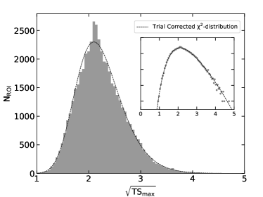
Figure 1: The $TS_{\rm max}$ distribution of 49152 searched ROIs. The dashed line is the best fit trial-corrected $\chi^{2}$ distribution. The inserted sub-figure is the same distribution plotted in a y-log framework for better showing the tails of the distribution.

In our all-sky searches, no signal is found to have a TS value greater than 25 ($TS=25$ corresponds to a local significance of $5\,\sigma$). The most significant line-like excess appears in the ROI centered on ($l=182.81$, $b=-15.09$), with a TS value of 24.3. The corresponding line energy is 74.9 GeV. The observation spectrum of this ROI can be found in Appendix C. Evidence of excess is clearly seen for this ROI, indicating that our search strategy can effectively identify such a kind of signal in the spectrum. Besides this excess, in total 50 ROIs give $TS_{\rm max}>16$ and 2953 result in $TS_{\rm max}>9$.

The 50 ROIs showing highest TS values are of particular interest to us, because they have higher probabilities of being from real signal rather than background fluctuation. We plot their positions in the sky in Figure 2. Though these regions have $TS_{\rm max}>16$, intrinsically their global significances are very low. The reason is that we have searched a lot of ROIs and for each ROI a series of line energies, an extremly large trial-factor is introduced if we convert the TS values to the global significances. Utilizing the null distribution in Figure 1 and attributing 49152 trials to the scan over multiple ROIs, the derived global significances are 0.54$\sigma$ and 0.11$\sigma$ for the first two ROIs with $TS_{\rm max}=24.3$ and $22.4$, respectively, and $<0.1\sigma$ for any other ROIs. These weak line-like excesses are most likely from statistical fluctuations. In view of the great importance of the line signal, these regions still deserve further attention. If one can find the same excesses in some of these regions by analyzing the data from other gamma-ray telescopes, the statistical origin will be disfavored. We thus present the information of the ROIs with $TS_{\rm max}>16$ in Appendix D, they can be treated as a list of potential line signal regions for later studies.

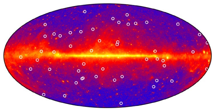
Figure 2: ROIs showing line-like excesses with $\rm TS>16$ overlaid on a Hammer-Aitoff projection of Fermi-LAT counts map ($E>1\,{\rm GeV}$).

IV Searching for counterparts of the weak line-like excesses

In addition to waiting for the observations from other instruments, we have also attempted to test the possible DM origin of these excesses by searching for their counterparts. The dark matter particles that generate the gamma-ray lines may simultaneously annihilate to other Standard Model particles (e.g., $b\bar{b}$, $\tau^{+}\tau^{-}$) Lefranc et al. (2016), which could yield continuum gamma-ray emission at lower energies. This model-independent gamma-ray emissions provide us a way to test the possible DM origin of the line-like excesses. Specifically, for a certain excess, if we could detect another gamma-ray component in the ROI with its spectrum and spatial distribution compatible with DM continuum emission, it is a strong evidence that both the line and continuum emission are from DM annihilation within a given subhalo. For this reason, we analyze the unassociated point sources within the ROIs of $TS_{\rm max}>16$. Due to the complicated gamma-ray backgrounds in the Galactic plane, we ignore the ROIs with latitudes $|b|<10^{\circ}$. Totally, 13 unassociated point sources in FL8Y are found. We apply the standard likelihood analysis of Fermi-LAT data to these unassociated sources in the energy range from 300 MeV to 300 GeV. The unassociated point sources are modeled with spectrum of DM annihilation and the spectral function adopted in FL8Y. For the DM model, we consider the annihilation channel of $b\bar{b}$ and $\tau^{+}\tau^{-}$, and the DM mass is fixed to the $E_{\gamma}$ giving the largest TS value in each ROI. The delta likelihood between these two models, $\Delta\ln{\mathcal{L}}=\ln{{\mathcal{L}}_{\rm DM}}-\ln{{\mathcal{L}}_{\rm FL8Y}}$, is used to determine whether a DM annihilation hypothesis is favored. Our analyses show that only 1 among 13 sources, FL8Y J1656.4-0410, marginally favors the DM spectrum over the spectral model used in FL8Y. The $\Delta\ln{\mathcal{L}}=7.0$ corresponds to a local significance of $<4\sigma$, not offering an evidence of DM signal from subhalo.

Besides, if certain of the line-like excesses in the Table 1 is a real DM signal, it could be from any channel of $\chi\chi\rightarrow\gamma\gamma$ or $\gamma{Z}$ or $\gamma{H}$, then it is possible that the dark matter particles also annihilate through another channel among the three Su and Finkbeiner (2012). For example, assuming the first line signal is from $\chi\chi\rightarrow\gamma\gamma$, the second line would be located at $E^{\prime}_{\gamma}=m_{\chi}(1-m_{X}^{2}/4m_{\chi}^{2})$, where $X$ could be $Z$ or $h$. If the second line is found with high significance, it also offers an indication that the line-like excess in Table 1 is a real DM signal. Thus for the 50 ROIs, we calculate the TS values of the second line signals at the corresponding energies. The largest TS values for the second lines are listed in Table 1 as well. We find that only 4 ROIs result in TS${}_{\rm 2nd}>4$, and the highest one appears in the ROI #35888. The combined TS of this ROI reaches 27.1 for the two gamma-ray lines, however considering additional degree of freedom and very large trial factors, the global significance is still very low.

V Constraining DM cross section with the non-detection of significant line signal

In the cold dark matter paradigm, structure forms hierarchically, and it is predicted that there exist large amount of DM subhalos around the Milky Way. Such a prediction is supported by numerical $N$-body simulations Diemand et al. (2008); Springel et al. (2008); Garrison-Kimmel et al. (2014). The concentration of DM in the subhalos leads to a higher DM annihilation rate. If massive subhalos are close to the Earth sufficiently, they may generate gamma-ray signals detectable by Fermi-LAT. For some subhalos which are too small to capture enough baryonic matter (i.e., $M_{\rm sub}<10^{8}\,M_{\odot}$), the gamma-ray annihilation signals would be the only channel to observe them. Thus, it is supposed that some unassociated Fermi-LAT sources are potential DM subhalos Ackermann et al. (2012c); Berlin and Hooper (2014); Bertoni et al. (2015); Schoonenberg et al. (2016); Bertoni et al. (2016); Hooper and Witte (2017); Calore et al. (2017); Wang et al. (2016); Xia et al. (2017), especially those spatially extended and with spectra compatible with DM signals Bertoni et al. (2016); Wang et al. (2016); Xia et al. (2017).

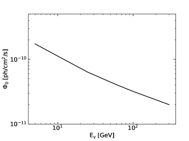
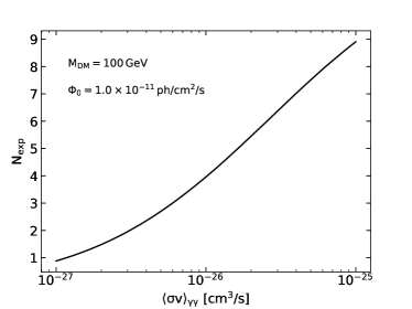
Figure 3: Left panel: The line signal detection threshold $\Phi_{0}$ as a function of the line energy $E_{\gamma}$. Right panel: The expected number of subhalos that can yield line signal significantly detectable by Fermi-LAT as a function of the line signal cross section assuming a DM mass of 100 GeV and a detection threshold of $1.0\times 10^{-11}\,{\rm ph/cm^{2}/s}$. Note that $\Phi_{0}$, $M_{\rm DM}$ and $\left<\sigma{v}\right>$ are actually three degenerate parameters, the curve in the right panel applies to any values of $\Phi_{0}$ and $M_{\rm DM}$.

No significant line signal ($TS>25$) is found in our analysis and we can set limits on the DM cross section of annihilating to gamma-rays, $\left<\sigma{v}\right>_{\gamma\gamma}$. The basic idea is that, higher cross section may lead to brighter gamma-ray annihilation flux that more subhalos far from us can be detected Ackermann et al. (2012c); Berlin and Hooper (2014); Bertoni et al. (2015); Schoonenberg et al. (2016); Hooper and Witte (2017); Calore et al. (2017). The number of expected observable subhalos $N_{\rm exp}$ is therefore proportional to the cross section. According to poisson statistics, for a model of $N_{\rm exp}$ observable subhalos, the probability distribution function of the number of detected subhalos, $N_{\rm obs}$, is

$$p(N_{\rm obs}|N_{\rm exp})=\frac{(N_{\rm exp})^{N_{\rm obs}}\exp^{-N_{\rm exp}}}{N_{\rm obs}!}.$$ (1)

Thus for a given number of real observed subhalos $N^{\prime}_{\rm obs}$, the 95% upper limit of $N_{\rm exp}$ corresponds to the one make

$$\int_{N_{\rm obs}>N^{\prime}_{\rm obs}}{p(N_{\rm obs}|N_{\rm exp})}{\rm d}N_{\rm obs}>0.95.$$ (2)

Since we do not find any line-like excesses with $TS>25$, we set $N^{\prime}_{\rm obs}=0$, leading to $N_{\rm exp}<3$ at 95% confidence level.

Here we use the expression derived in Ref. Hooper and Witte (2017) (hereafter H16) to give the predicted numbers of the observable DM subhalos,

$$N_{\text{exp}} = \Omega\int\int\int\int D^{2}\,\frac{dN}{dMdV}\,\frac{dP}{d\gamma}\,\frac{dP}{dR_{b}}\,$$

$$\Theta[\Phi_{\gamma}(M,D,R_{b},\gamma)-\Phi_{0}]\,dM\,dD\,dR_{b}\,d\gamma,$$

where $D$ and $M$ are the distance and mass of subhalo, respectively. The gamma-ray flux of the line signal generated in a given subhalo is

$$\Phi_{\gamma}=\frac{{\langle\sigma v\rangle}_{\gamma\gamma}}{4\pi m^{2}_{\chi}D^{2}}\int\rho^{2}(r)\,dV.$$ (4)

For the DM distribution in the subhalo $\rho(r)$, following H16, a density profile of power law with exponetial cutoff (PLE) is adopted rather than the Navarro-Frenk-White Navarro et al. (1997) one,

$$\rho(r)=\frac{\rho_{0}}{r^{\gamma}}\,\exp\left(-\frac{r}{R_{b}}\right)\,.$$ (5)

It is found that a PLE density profile can better match the characteristics found in the VL-II and ELVIS simulations considering the effects of tidal stripping Hooper and Witte (2017). In Eq. (LABEL:eq:npred), the $dN/dMdV$, $dP/d\gamma$ and $dP/dR_{b}$ are subhalo distribution and the distributions of the values of $\gamma$ and $R_{b}$ near the Earth’s location. For these distributions we also utilize the formulae reported in H16, which are presented in Appendix A as well. When deriving the distributions, their dependence on both the subhalo mass and the location relative to the galactic center has been taken into account Hooper and Witte (2017). Please note that these distributions in the integrand of Eq. (LABEL:eq:npred) are only valid in the local environment; especially, to simplify the calculation, a uniform subhalo number density ($dN/dV\propto$const) is assumed following H16. We thus consider only the subhalos within the distance of $5\,{\rm kpc}$ . Subhalos at larger distances may also be detectable, our choice of $D_{\rm max}$ will lead to relatively conservative results.

The $\Phi_{0}$ in Eq. (LABEL:eq:npred) denotes the flux threshold above which the line signals will be significantly detected. Since no line signal is found with $TS>25$, we make use of the Monte Carlo simulation to derive the $\Phi_{0}$. We model the Fermi-LAT observation spectrum averaged over all the sky (excluding the Galactic plane and the regions around bright gamma-ray sources, see below) with a PLE function and use this PLE spectrum to approximate the backgrounds in our line searches. Based on this PLE background spectrum, we generate pseudo photons in the 2^∘ ROI. Besides, a line-like component is superposed onto the background, the profile of which is the energy dispersion function of the Fermi-LAT data used in this work. We apply the same searching procedure as that in Sec. II on these pseudo data, and derive corresponding TS value of the line component. By varying the flux $\Phi$ of the input line component, for each $E_{\gamma}$ we determine the threshold above which the line component has a TS value greater than 25. We perform 100 Monte Carlo simulations and adopt the median value of the thresholds as the $\Phi_{0}$. The resultant $\Phi_{0}$ curve is shown in the left panel of Figure 3.

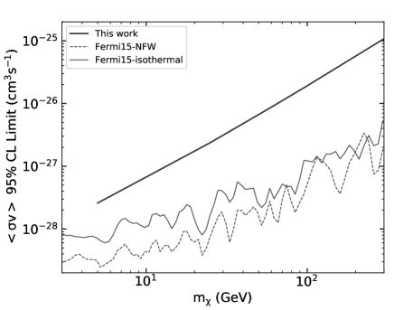
Figure 4: The 95% confidence level upper limits on the cross sections of DM annihilating into double $\gamma$-rays derived in our analysis. As a comparison, we also plot the constraints set by the Fermi-LAT observations of the Galactic central regions Ackermann et al. (2015).

The background gamma-ray emissions in the Galactic plane region and near bright gamma-ray point sources are much stronger than that in other regions, thus lowering the detectability of a line signal from subhalo. In this section, for both calculating the observed solid angle $\Omega$ and deriving the flux threshold $\Phi_{0}$, the regions of $|b|<20^{\circ}$ and those within $2^{\circ}$ around the 100 most bright point sources in 3FGL Acero et al. (2015) are excluded.

With the elements described above, we can calculate the expected number of subhalos, $N_{\rm exp}$, that can yield line signals significantly detectable by Fermi-LAT. Assuming a detection threshold of $\Phi_{0}=1.0\times 10^{-11}\,{\rm ph\,cm^{-2}\,s^{-1}}$, the $N_{\rm exp}$ as a function of cross section for 100 GeV DM is shown in the right panel of Figure 3. We apply poisson statistics to the $N_{\rm exp}$ (i.e., requiring $N_{\rm exp}<3$) to place a 95% upper limit on the annihilation cross section for a given value of the DM mass. The obtained constraints are shown in Figure 4. As a comparison, also plotted are the constraints derived based on the Fermi-LAT observation towards the regions around the Galactic center Ackermann et al. (2015). We find that our constraints here are not competitive with these Galactic ones (thin solid line for the isothermal density profile and dashed line for the NFW). We would like to emphasize that in the calculation we have considered only the subhalos within 5 kpc. The current constraints would be improved by including the subhalos farther away.

VI Summary

In this work, we have analyzed the Fermi-LAT data to blindly search for the potential line signals originated from anywhere of the sky. We make use of the sliding window technique to perform unbinned likelihood fittings in 49152 ROIs, which cover the whole sky. We did not find line signal with $TS>25$. However, line-like excesses with $TS>16$ appear in the spectra of 50 regions. After the trial factor correction, the highest global significance among these excesses is only $0.54\sigma$. These excesses are most likely originated from statistic fluctuations. In any case, the possibility that very a few of them come from DM annihilation can not be excluded. If one can analyze the data observed by other/future survey mode gamma-ray observatories in the same regions, their origin (DM or statistical fluctuation) may be identified. We thus suggest that these regions are worth further attention. All these regions have been presented in Appendix D.

The DM particles that generate the line signals may simultaneously annihilate through other channels, thus leading to counterpart gamma-ray emission (either continuum emission at lower energies or a second gamma-ray line). If detected, these counterparts provide indications of DM origin of the line signals. In Section IV, we have attempted to search for the counterpart gamma-ray emissions for the line-like excesses in Table 1 by analyzing the Fermi-LAT unassociated point sources within selected ROIs (for continuum emission) or by examining the significances of the second lines at specific energies. No evidence of the counterparts is found in the analyses.

Some previous works have pointed out that the number of DM subhalo candidates can be used to place constraints on the DM cross section. In our analysis, we don’t find any significant line signal with $TS>25$, then the number of observed subhalo is zero. Based on this, we derive the expected number of subhalos as a function of the cross section of DM annihilating to gamma-ray lines, and then set constraints on the latter. We found that the constraints obtained here are weaker than those given according to the Fermi-LAT observations towards the Galactic central region. Nevertheless our work offers a novel approach to support these previous constraints independently.

Finally, we would point out that some other on-orbit or proposed space borne gamma-ray telescopes, such as DAMPE Chang et al. (2017), Gamma-400 Galper et al. (2014) and HERD Zhang et al. (2014), all of which have significantly better energy resolution comparing to Fermi-LAT, will contribute significantly to the gamma-ray line search and may help examining the origin of the line-like excesses in this work.

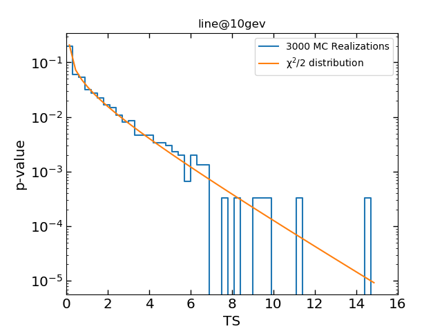
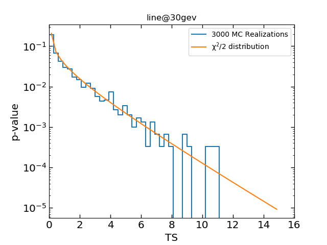
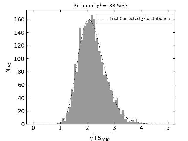
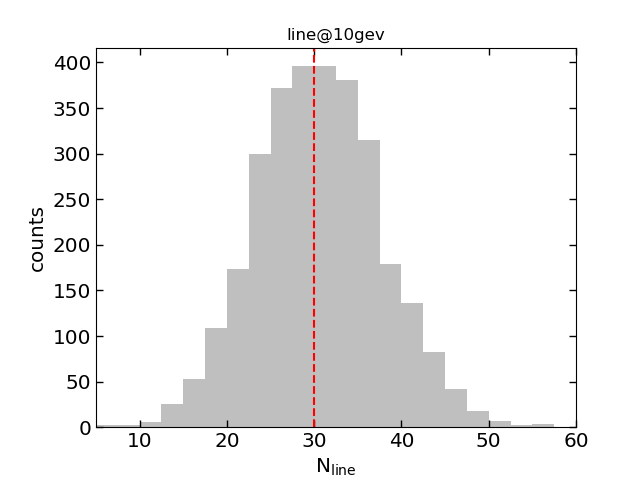
Figure 5: Top: Distribution of TS values from individual fits of a 10 GeV (left panel) or 30 GeV (right panel) line to the 3000 background-only simulations. Bottom left: The $TS_{\rm max}$ distribution of 3000 Monte Carlo spectra generated from background-only simulations. The dashed line is the best fit trial-corrected $\chi^{2}$ distribution. Bottom right: We inject a pesudo line signal with photon number $N_{\rm line}=30$ at 10 GeV into the MC data and fit them with background+line model. This plot shows that our fits can well recover the input parameter (red line).

Appendix A Subhalo distribution and the distributions of $\gamma$ and $R_{b}$

The subhalo distribution and the distributions of $\gamma$ and $R_{b}$ adopted in our analysis are from Ref. Hooper and Witte (2017). When deriving the distributions, their dependences on both the subhalo mass and the location relative to the galactic center have been taken into account Hooper and Witte (2017). The subhalo distribution is

$$\frac{dN}{dMdV}=\frac{628}{M_{\odot}\,{\rm kpc}^{3}}\left(\frac{M}{M_{\odot}}\right)^{-1.9}\,.$$ (6)

The distributions of $R_{b}$ is

$$\frac{dP}{dR_{b}} = \frac{1}{\sigma\sqrt{2\pi}}\,\frac{1}{R_{b}}\exp\left(-\frac{(\ln R_{b}-\ln\langle R_{b}\rangle)^{2}}{2\sigma^{2}}\right),$$ (7)

where $\sigma=0.496$ and $\langle R_{b}\rangle=10^{-3.945}\times(M/M_{\odot})^{0.421}$. The distributions of $\gamma$ is found to be independent of subhalo mass and is expressed as

$$\frac{dP}{d\gamma} = \frac{1}{\sqrt{2\pi}}\,\frac{1}{\sigma-\kappa(\gamma-\langle\gamma\rangle)}\times$$ (8)

$$\exp\left(-\frac{\ln^{2}(1-\kappa(\gamma-\langle\gamma\rangle)/\sigma)}{2\kappa^{2}}\right),$$

with $\langle\gamma\rangle=0.74$, $\sigma=0.42$ and $\kappa=0.10$.

Appendix B Validity of the search method

In this section we carry out some Monte Carlo (MC) simulation to test the validity of the method to search for the line (sliding window technique, unbinned analysis, etc.).

We first simulate background-only data, and fit them with the background+line model to examine the null distribution. We model the Fermi-LAT observation spectrum averaged over all the sky (excluding the Galactic plane and the regions around bright gamma-ray sources, see Section V) with a PLE function and use this PLE spectrum to approximate the backgrounds in our line searches. Based on this PLE background spectrum, we generate pseudo photons in 2^∘ ROI according to Poisson statistics. We apply the same search procedure as that in Sec. II on these pseudo data, and derive corresponding TS values of the line component. As predicted by the asymptotic theorem of Chernoff Chernoff (1954), for individual $E_{\gamma}$, the distribution of the TS values (null distribution) should follow a $\chi^{2}/2$ distribution. From the top panels of Figure 5, we find that the TS distribution derived from 3000 MC simulations is well consistent with matched to the theoretical prediction for two representative line energies of 10 GeV and 30 GeV. Applying sliding window fit to the 3000 MC spectra and deriving the $TS_{\rm max}$ of them, we obtain the distribution shown in the bottom-left panel of Figure 5. Unlike significant deviation around $TS_{\rm max}\sim 4-5$ displaying in Figure 1, the trial-corrected $\chi^{2}$ distribution can lead to a good fit (reduced-$\chi^{2}=33.5/33$) to the $TS_{\rm max}$ distribution of simulation data.

Furthermore, we inject a line component with intensity of 30 photons, of which the profile is the energy dispersion function of the Fermi-LAT data used in this work, into the background to generate MC events containing a fake line signal. We apply the search analysis to these events to re-derive the photon number / flux of the line component. We find that the input parameter of $N_{\rm line}=30$ can be well recovered (bottom-right panel of Figure 5).

The results presented in this section indicate our search method/code are valid to search for a line signal from the background and the deviation around $TS_{\rm max}\sim 4-5$ appeared in Figure 1 is most-likely irrelevant to the analysis procedure.

Appendix C The spectrum of the ROI giving highest TS value

Figure 6 presents the Fermi-LAT spectrum of the ROI giving the highest $TS_{\rm max}$ in our analysis. The excess is seen around energy of 74.9 GeV, indicating that our analysis can effectively identify such a kind of signal in the spectrum. We would like to emphasize that the binned plots in Figure 6 are just for illustration, while in the search procedure of the main text an unbinned method is adopted.

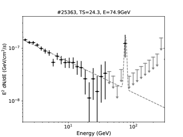
Figure 6: The observed spectrum of the ROI displaying line-like excess with $TS=24.3$, which is the highest one in our analysis. For the energy bins with photon number less than 2, we plot $1\sigma$ confidence level upper limits for better visualization. Note that the line-like excess shown here is most likely from background fluctuation since a very large trial factor is introduced in the analysis.

Appendix D Information of 50 ROIs with $TS_{\rm max}>16$

As discussed in the main text, we think the 50 ROIs with relative high significances of $TS_{\rm max}>16$ deserve further attention. Then we list them in Table 1 for later studies. Their positions in the sky are shown in Figure 2. Note that since the radius of the adopted ROI ($2^{\circ}$) is larger than the interval between two ROI centers, it is possible that several ROIs contain the same excess. In such a case we only retain the ROI with the largest TS value.

Table 1: Line-like excesses with $\rm TS>16$ identified in this work.

#	Energy [GeV]	TS Value	TS2nd	LON [∘]	LAT [∘]	RA [∘]	Dec [∘]
25363	74.9	24.3	0.0	182.81	-15.09	74.40	18.21
21714	17.5	22.4	0.1	114.61	-5.98	357.97	55.93
9695	29.2	21.5	3.8	269.15	50.48	171.98	-6.83
45226	16.2	21.0	0.0	272.81	-78.28	20.20	-37.07
15172	48.6	20.1	6.3(91.3)	296.32	50.48	188.56	-12.17
24414	9.4	20.0	1.2	97.73	31.39	265.83	67.66
34394	18.2	19.6	0.9	62.58	-41.81	332.47	1.38
18272	38.4	19.6	5.8(68.7)	25.31	7.78	272.45	-3.16
37762	5.2	19.5	1.8	125.36	-58.92	14.11	3.93
36744	5.8	19.1	3.2	37.97	-12.64	296.38	-1.35
278	27.0	18.8	0.6	59.77	14.48	281.32	30.20
36061	66.6	18.6	0.0	48.52	-23.32	310.58	2.24
35642	5.6	18.6	0.8	20.39	-32.80	308.78	-24.17
42727	5.4	18.5	2.3	234.84	-34.95	76.89	-32.24
46981	8.7	18.3	0.0	333.98	-32.80	302.38	-62.61
40543	11.8	18.3	0.8	132.19	-17.58	25.25	44.40
20889	50.6	18.1	3.6	97.73	-19.47	342.51	37.39
29481	38.4	18.0	0.8	266.48	-14.48	115.85	-53.82
35865	27.0	18.0	3.9	47.11	-35.69	320.62	-5.10
10660	5.2	18.0	1.0	206.72	41.01	138.95	21.83
20103	35.5	17.9	3.5	344.53	17.58	239.68	-29.78
14243	10.5	17.8	0.0	333.37	53.57	210.44	-5.09
35888	26.0	17.6	9.5(60.4)	45.00	-34.95	319.13	-6.24
7168	9.0	17.6	2.8	135.00	42.61	163.57	71.67
14313	66.6	17.3	1.3	345.37	60.43	212.36	4.16
29638	13.3	17.2	1.6	270.70	-7.18	130.02	-53.51
16786	11.8	17.2	0.2	7.73	-20.74	291.84	-31.05
7867	8.0	17.1	1.2	91.67	70.17	206.89	43.40
28138	31.6	17.1	4.1(64.1)	186.33	24.62	115.70	33.53
1666	37.0	17.0	1.3	49.92	37.17	253.34	28.86
27865	5.4	17.0	0.0	182.11	14.48	102.60	33.75
42296	29.2	17.0	0.0	260.08	-45.78	62.38	-51.43
30431	10.5	16.9	2.3	284.06	6.58	161.66	-51.66
30245	13.3	16.8	0.5	280.55	-4.78	145.21	-59.10
19922	31.6	16.8	0.9	13.36	23.32	253.21	-5.35
46538	35.5	16.8	3.6	346.64	-38.68	311.85	-51.92
6201	35.5	16.8	1.8	111.80	27.28	279.44	80.10
29823	6.1	16.8	0.5	298.12	-5.38	180.12	-67.77
38012	29.2	16.7	0.5	168.96	-50.48	40.14	2.38
24463	9.0	16.6	0.9	84.37	29.31	269.93	56.11
28712	12.3	16.5	1.1	265.78	-36.42	76.96	-57.30
22401	21.3	16.3	0.0	107.58	5.98	335.47	64.30
2458	10.5	16.2	0.3	28.83	41.81	243.14	14.86
1240	46.8	16.2	1.5	68.91	34.95	259.22	43.61
15976	45.0	16.1	2.4	295.91	65.70	189.97	2.98
26070	74.9	16.1	0.0	217.27	4.78	109.09	-1.66
23595	12.3	16.1	0.4	85.78	5.38	307.71	48.50
20147	9.7	16.0	3.3	343.12	21.38	235.67	-27.83
15410	9.7	16.0	0.2	314.17	49.70	200.28	-12.52
27195	59.2	16.0	1.4	144.84	-1.79	52.47	54.20