Low-Overhead Hierarchically-Sparse Channel Estimation for Multiuser Wideband Massive MIMO

Abstract

Numerical evidence suggests that compressive sensing (CS) approaches for wideband massive MIMO channel estimation can achieve very good performance with limited training overhead by exploiting the sparsity of the physical channel. However, analytical characterization of the (minimum) training overhead requirements is still an open issue. By observing that the wideband massive MIMO channel can be represented by a vector that is not simply sparse but has well defined structural properties, referred to as hierarchical sparsity, we propose low complexity channel estimators for the uplink multiuser scenario that take this property into account. By employing the framework of the hierarchical restricted isometry property, rigorous performance guarantees for these algorithms are provided suggesting concrete design goals for the user pilot sequences. For a specific design, we analytically characterize the scaling of the required pilot overhead with increasing number of antennas and bandwidth, revealing that, as long as the number of antennas is sufficiently large, it is independent of the per user channel sparsity level as well as the number of active users. These analytical insights are verified by simulations demonstrating also the superiority of the proposed algorithm over conventional CS algorithms that ignore the hierarchical sparsity property.

I Introduction

Massive mutliple-input multiple-output (MIMO) is the term used to describe the practice of deploying a large number of antennas at the base station (BS), which is considered as a key technology for 5G [2]. Although the benefits of massive MIMO are by now well understood [3], the fundamental bottleneck for massive MIMO deployment in a multi-cell scenario is pilot contamination, i.e., degradation of the uplink channel state information (CSI) due to multiple user equipments (UEs) transmitting non-orthogonal training signals on the same set of resources [4]. In addition, with the emergence of massive machine type communications (MTCs) with typically small data bursts, there is a need to decrease the signaling overhead associated with the CSI acquisition [5], thus resulting in pilot contamination issues also in a single-cell scenario. It is therefore of critical importance to come up with designs that balance the conflicting requirements of accurate CSI and low training overhead, for systems with a massive number of antennas, UEs, and bandwidth.

I-A Related Work

The topic of (optimal) training design and channel estimation for the single UE case has been extensively studied for the multi-antenna and/or wideband (OFDM) channels both from an estimation mean squared error (MSE) as well as a capacity perspective (see, e.g., [6, 7, 8, 9]). This line of works on pilot-aided system design was based on the assumption of a rich scattering propagation environment, effectively treating the channel response among different antennas as independent. This results in pilot designs having a training overhead that is proportional to the product of the number of antenna elements and the system bandwidth. Application of these approaches in the multiuser setting may be unacceptable due to limited resources that cannot allow for orthogonal pilot transmissions, resulting in pilot contamination effects [4, 10].

The key towards reducing the training overhead is the observation that the wireless channel is fundamentally sparse, i.e., a signal arrives at the receiver via a limited number of distinct (resolvable) paths [11]. This propagation has been experimentally observed to hold true with large carrier frequencies (beyond 2GHz) and/or with large antenna array (i.e., massive MIMO) [12]. Therefore, posing the channel estimation problem as that of identifying the channel paths properties (gain, delay, angle) immediately implies improvement of the CSI procedure over the conventional approaches, either in terms of performance (MSE) or training overhead, as the number of unknowns to be estimated (significantly) decreases.

Earlier works exploiting this channel sparsity for estimation purposes (e.g., [13]) utilized traditional tools from the fields of array processing and harmonic retrieval [14], however, the focus was only on algorithmic and performance aspects, and the issue of training overhead minimization was ignored. The recent advent of the field of compressive sensing (CS) [15], which considers the problem of solving an under-determined linear system under the assumption that the vector to be estimated is sparse, has provided a new set of tools towards low-overhead sparse channel estimation [16]. Considering the problem of wideband massive MIMO channel estimation, by reformulating it in a format compatible to the one considered in CS, a few recent publications have proposed CS-inspired channel estimation algorithms demonstrating that excellent performance is indeed possible with low training overhead [17, 18]. However, these performance results are only provided via means of numerical simulations, with very limited (if at all) analytical insights on the training overhead required to achieve a certain performance. A different approach is considered in [19], where it is the (sparse) covariance matrix of the channel that is estimated by a CS approach, with the resulting estimate used to perform linear minimum mean squared error (LMMSE) channel estimation. However, this approach requires the observation of multiple, independent channel snapshots, which might not be possible under certain scenarios (e.g., short length MTCs).

Intuitively, one expects that the utilization of multiple antennas at the BS can aid in reducing the bandwidth dedicated for training signals. However, to the best of our knowledge, there are no analytical results available that confirm this intuition, even though CS theory provides numerous rigorous answers regarding number of measurements required to achieve good estimation performance [20]. This lack of analysis in the considered setup is mainly due to the, so called, sensing matrix of the corresponding CS problem formulation having a Kronecker-product structure [23]. Even though Kronecker-product sensing matrices have been explicitly investigated in the CS literature [21, 22], the available results suggest a required training overhead that is overly pessimistic (cf. discussion of Theorem 9).

I-B Contributions

In this paper, a setup with a single BS equipped with a uniform linear array (ULA) serving multiple single-antenna uplink UEs is considered, with the goal of proposing efficient channel estimation algorithms as well as providing rigorous analytical insights on the overhead requirements. Under the assumption of, so called, on-grid channel parameters, that is reasonable for asymptotically large number of antennas and bandwidth, a key observation is that the channel estimation problem can be formulated as the CS estimation of a vector that is not simply sparse but hierarchically sparse [25, 26, 27, 28]. In particular, the positions of its non-zero elements cannot be arbitrary but are subject to constraints implied by the physical channel properties. This is a critical property that is exploited in the following.

The main contributions of the paper are summarized as follows.

• Two novel, low-complexity channel estimation algorithms are proposed that explicitly take into account the hierarchical sparsity property, which was ignored in the previous literature. The algorithm description is provided for an arbitrary pilot sequence design, where multiple UEs utilize the same subcarriers of a single OFDM symbol for training purposes.

• The notion of the hierarchical restricted isometry property (HiRIP) is introduced, which can be considered as a specialization of the standard RIP notion [20] to the setting of hierarchically sparse vectors. Rigorous guarantees for reliable, i.e., bounded error, channel estimation by the proposed algorithms are provided based on the, so called, HiRIP constant of the Kronecker-product type sensing matrix of the corresponding CS estimation problem.

• The above characterization provides a concrete design goal for the pilot sequence design, namely, it should be such that the HiRIP constant of the sensing matrix is sufficiently small. Towards this, a design based on phase-shifted UE pilot sequences is proposed, which allows for a rigorous description of the scaling of the number of pilot subcarriers and number of observed antennas required to achieve reliable channel estimation. The analysis highlights the benefit of using multiple antennas in the sense of allowing for reduced pilot-overhead compared to the single antenna case. Even more important, for sufficiently large number of antennas, the pilot overhead required is independent of the number of (active) UEs and number of channel paths per UE. These conclusions are verified by numerical simulations demonstrating also the superior performance of the proposed algorithms compared to standard CS algorithms of comparable complexity that ignore hierarchical sparsity. The latter requires a significantly larger minimum pilot overhead to achieve reasonable performance that also increases with number of channel paths per UE.

• The cases of jointly processing multiple training OFDM symbols as well as channels with off-grid parameters is also discussed, as both can be naturally accommodated by the proposed framework. Simulations show that in the latter case, although the mismatch of assuming on-grid channel parameters by the algorithm results in a performance degradation, performance remains still significantly better in terms of required overhead compared to standard CS algorithms of comparable complexity as well as the conventional linear minimum mean square error (LMMSE) estimator that ignores channel sparsity altogether.

I-C Notation

Vectors and matrices will be denoted by lower and upper case bold letters, respectively. All vectors are column vectors. The $(n,m)$ element of $\mathbf{X}\in\mathbb{C}^{N\times M}$ is denoted by $[\mathbf{X}]_{n,m},n\in[N],m\in[M],$ with $[N]\triangleq\{0,1,\ldots,N-1\}$. $(\cdot)^{*},(\cdot)^{T},(\cdot)^{H}$ denote complex conjugate, transpose, and Hermitian operation, respectively. $\lVert\mathbf{X}\rVert\triangleq\sqrt{\text{tr}\{\mathbf{X}^{H}\mathbf{X}\}}$ is the Frobenius norm (Euclidean norm if $\mathbf{X}$ is a vector). The cardinality of a set $\mathcal{A}$ is denoted by $|\mathcal{A}|$. $\mathbf{X}_{\mathcal{A}}$ ($\mathbf{x}_{\mathcal{A}}$) denotes the matrix (vector) obtained either by extracting the rows (elements) of $\mathbf{X}$ ($\mathbf{x}$) enumerated by $\mathcal{A}\subseteq[N]$ or by setting the rows (elements) of $\mathbf{X}$ ($\mathbf{x}$) that do not belong to $\mathcal{A}$ equal to zero (the case will be clear from the context). The $N\times N$ identity matrix is denoted by $\mathbf{I}_{N}$ and $\text{diag}(\mathbf{x})$ denotes the diagonal matrix with $\mathbf{x}$ on its diagonal. $\mathbf{F}_{N,M}$ denotes the matrix obtained by the first $M\leq N$ columns of the $N\times N$ DFT matrix, i.e., $[\mathbf{F}_{N,M}]{}_{n,m}\triangleq e^{-j2\pi mn/N},n\in[N],m\in[M]$. The vector resulting of stacking the columns of a matrix $\mathbf{X}$ is denoted by $\text{vec}(\mathbf{X})$. $\text{supp}(\mathbf{x})\subseteq[N]$ denotes the set of non-zero elements (support) of $\mathbf{x}\in\mathbb{C}^{N}$. $\mathbb{C}^{N_{1}\cdot N_{2}\cdots N_{\ell}}$ denotes the space of complex-valued, multilevel block vectors consisting of $N_{1}$ blocks, each containing $N_{2}$ blocks, $\ldots$, each containing $N_{\ell-1}$ blocks of $N_{\ell}$ elements (for a total of $N_{1}N_{2}\cdots N_{\ell}$ elements). A vector $\mathbf{x}$ is called $s$-sparse if $|\text{supp}(\mathbf{x})|=s$. For reference, the following standard definition from CS theory [20] is recalled below.

Definition 1 (RIP constant).

The restricted isometry constant $\delta_{s}(\mathbf{A})$ of a (deterministic) matrix $\mathbf{A}\in\mathbb{C}^{N\times M}$ is the smallest $\delta\geq 0$ such that

$$(1-\delta)\|\mathbf{x}\|^{2}\leq\|\mathbf{A}\mathbf{x}\|^{2}\leq(1+\delta)\|\mathbf{x}\|^{2},$$ (1)

for all $s$-sparse vectors $\mathbf{x}\in\mathbb{C}^{M}$ ($s\leq M$). We say that $\mathbf{A}$ satisfies the ($s$-th) restricted isometry property ($s$-RIP) if $\delta_{s}(\mathbf{A})<\bar{\delta}$ where $\bar{\delta}<1$ is a pre-specified constant.

II Wideband Massive MIMO Channel Model and Delay-Angular Representation

We consider the uplink of a single cell with a BS equipped with $M\gg 1$ antenna elements serving multiple single-antenna UEs. For a ULA, the array manifold $\mathbf{a}\left(\cdot\right):\left[-\pi/2,\pi/2\right]\rightarrow\mathbb{C}^{M}$, which maps angular to spatial domain, is given by $\mathbf{a}\left(\phi\right)\triangleq[1,e^{-j2\pi d\sin\phi},\ldots,e^{-j2\pi d\left(M-1\right)\sin\phi}]^{T}$ [24]. Here, $d$ is the normalized spatial separation of the ULA (with respect to carrier wavelength), which, without loss of generality (w.l.o.g.), is assumed to be equal to $1/2$ in the following. As is routinely done, we perform the change of variable $\theta=d\sin(\phi)\in[-1/2,1/2]$ and, with a slight abuse of notation, we write the array manifold as a function of $\theta$, i.e., $\mathbf{a}\left(\theta\right)=[1,e^{-j2\pi\theta},\ldots,e^{-j2\pi\left(M-1\right)\theta}]^{T}$. Noting that $\mathbf{a}(\theta)=\mathbf{a}(1-\theta)$ for $\theta<0$, it is convenient to treat $\theta$ as taking values in $[0,1]$. Considering a sampled version of this interval by the $M$ points $\{k/M\}_{k=0}^{M-1}$ yields the steering (dictionary) matrix $\mathbf{A}_{\theta}\triangleq\left[\mathbf{a}(0),\mathbf{a}(1/M),\ldots,\mathbf{a}((M-1)/M)\right]=\mathbf{F}_{M,M}\in\mathbb{C}^{M\times M}$.

Transmissions are performed via wideband OFDM signals with $N\gg 1$ subcarriers centered at the baseband frequencies $\{2\pi k/T_{s}\}_{k=0}^{N-1}$, with $T_{s}>0$ being the useful (without the cyclic prefix) OFDM symbol duration. Assuming that the maximum delay spread of all UE channels is not longer than $\alpha T_{s},\alpha\leq 1$, which is the case in any reasonable OFDM design, the delay manifold $\mathbf{b}\left(\cdot\right):\left[0,\alpha T_{s}\right]\rightarrow\mathbb{C}^{N}$, which maps the delay to the frequency domain, is defined as $\mathbf{b}\left(\tau\right)\triangleq[1,e^{-j2\pi\tau/T_{s}},\ldots,e^{-j2\pi(N-1)\tau/T_{s}}]^{T}$ [24]. Considering a sampled version of $[0,T_{s}]$ by the $N$ points $\{kT_{s}/N\}_{k=0}^{N-1}$, yields the steering (dictionary) matrix $\mathbf{A}_{\tau}\triangleq\left[\mathbf{b}(0),\mathbf{b}(T_{s}/N),\ldots,\mathbf{b}((D-1)T_{s}/N)\right]=\mathbf{F}_{N,D}\in\mathbb{C}^{N\times D}$ where $D\triangleq\lfloor\alpha N\rfloor$ is the channel delay spread in samples.

The channel of an arbitrary UE is a superposition of a small number $L$ of impinging wavefronts (paths) characterized by their delay/angle pairs $\{(\tau_{p},\theta_{p})\}_{p=0}^{L-1}$, with $\tau_{p}\in[0,\alpha T_{s}]$, $\theta_{p}\in[0,1]$. This is reflected in the channel transfer matrix $\mathbf{H}\in\mathbb{C}^{N\times M}$ whose $(n,m)$-th element corresponds to the complex channel gain at subcarrier $n$ and antenna $m$ and can be written as [19, 24]

$$\mathbf{H}=\sum_{p=0}^{L-1}\rho_{p}\mathbf{b}\left(\tau_{p}\right)\mathbf{a}^{H}\left(\theta_{p}\right),$$ (2)

where $\rho_{p}\in\mathbb{C}$ is the complex gain of the $p$-th path. It is noted that $L$ is treated here as a given parameter that depends only on the physical propagation properties and is independent of system parameters $M$ and $N$.

Targeting low-complexity channel estimation, it is beneficial to consider an alternative representation of $\mathbf{H}$, which translates the physical sparsity to sparsity of an appropriately defined matrix that is to be identified by the estimator. Towards this end, we will first consider the case of on-grid channel parameters, when every delay/angle pair lies exactly on the delay/angle grid corresponding to the steering matrices $\mathbf{A}_{\theta}$ and $\mathbf{A}_{\tau}$, i.e., it holds $(\tau_{p},\theta_{p})=(k_{p}T_{s}/N,l_{p}/M)$ for some $k_{p}\in[D]$ and $l_{p}\in[M]$, for all $p\in[L]$. In general, this assumption does not hold, however, it is a reasonable approximation for asymptotically large $N$, $M$, and is convenient for algorithm design and (asymptotic) performance analysis. The more general, off-grid channel parameters case will be treated in Sec. V. Note that, apart from the on-grid/off-grid delay/angle pairs characterization, no assumptions on the (joint) statistics of path delays, angles, and gains are considered in the following treatment.

With on-grid parameters, $\mathbf{H}$ can then be written as

$$\mathbf{H}=\mathbf{A}_{\tau}\mathbf{X}\mathbf{A}_{\theta}^{H},$$ (3)

where

$$\mathbf{X}\triangleq\sum_{p=0}^{L-1}\rho_{p}\mathbf{e}_{k_{p},D}\mathbf{e}_{l_{p},M}^{T}\in\mathbb{C}^{D\times M},$$ (4)

with $\mathbf{e}_{n,N}\in\mathbb{C}^{N\times 1}$ denoting the canonical basis vector with the $n$-th element equal to $1$. Matrix $\mathbf{X}$ is the delay-angular representation of the channel, which is a sparse matrix with $L$ nonzero elements out of a total $DM$. An example of $\mathbf{X}$ with on-grid channel parameters is shown in Figure 1 (left panel). This sparsity of $\mathbf{X}$ (or its corresponding covariance matrix) has been exploited in the literature for obtaining efficient channel estimators [17, 18, 19] by direct application of algorithms from the field of CS. However, as will be argued in the following, the sparsity pattern (support) of $\mathbf{X}$ is not completely random but follows a hierarchical pattern, a property that will be exploited for algorithm design and rigorous analysis in terms of performance and overhead required to achieve it.

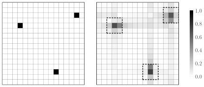
Figure 1: Example heatmap (modulus values) for the delay-angular representation $\mathbf{X}$ of a channel with $L=3$ and $\rho_{p}=1$ for all $p\in[L]$, and $N=M=D=16$. Left: on grid case; Right: off-grid case, obtained by slight perturbation of the angle/delay pairs values of the on-grid case.

III Multiuser Channel Estimation Problem Statement

Towards reducing the pilot overhead, the BS partitions the uplink UEs to groups of $U$ UEs. Each group is assigned an exclusive set of pilot subcarriers and all $V\leq U$ active UEs within a group transmit their pilots on these subcarriers and on the same OFDM symbol. For the analysis and design purposes, we consider an arbitrary UE group and discuss later the joint assignment of subcarriers to multiple groups. Let $\mathcal{N}_{p}\subseteq[N]$ denote the set of $N_{p}\triangleq|\mathcal{N}_{p}|$ dedicated pilot subcarriers to this group. Towards reducing implementation complexity, only the received signals from a set $\mathcal{M}_{p}\subseteq[M]$ of $M_{p}\triangleq|\mathcal{M}_{p}|$ antennas are considered at the BS for channel estimation purposes.

Let $\mathbf{P}_{\mathcal{N}_{p}}\triangleq\mathbf{I}_{N,\mathcal{N}_{p}}\in\{0,1\}^{N_{p}\times N}$ and $\mathbf{P}_{\mathcal{M}_{p}}\triangleq\mathbf{I}_{M,\mathcal{M}_{p}}\in\{0,1\}^{M_{p}\times M}$ denote the sampling matrices in frequency and space, respectively. The task of the BS is to identify all the UE channels from the observation

$$\mathbf{Y}=\sum_{u=0}^{U-1}\text{diag}(\mathbf{c}_{u})\mathbf{P}_{\mathcal{N}_{p}}\mathbf{H}_{u}\mathbf{P}_{\mathcal{M}_{p}}^{T}+\mathbf{Z}\in\mathbb{C}^{N_{p}\times M_{p}},$$ (5)

where $\mathbf{c}_{u}\in\mathbb{C}^{N_{p}},\mathbf{H}_{u}\in\mathbb{C}^{N\times M}$, are the pilot signature and channel transfer matrix of the $u$-th UE, respectively, and $\mathbf{Z}\in\mathbb{C}^{N_{p}\times M_{p}}$ is a noise matrix of arbitrary distribution apart from the mild assumption that $\|\mathbf{Z}\|$ is finite with probability $1$. The elements of $\mathbf{c}_{u}$ are known to the BS and assumed, w.l.o.g., to be of unit modulus for all $u\in[U]$. For the $U-V$ UEs that are not active, the channel transfer matrix is equal to an all-zeros matrix. The receiver is not aware which UEs are inactive but does know $V$ as well as the number of channel paths $L$, assumed to be the same for all UEs.

It follows from the discussion of Sec. II that the problem of estimating the transfer matrices $\{\mathbf{H}_{u}\}_{u\in[U]}$ can be equivalently posed as the problem of estimating the delay-angular channel representations $\{\mathbf{X}_{u}\}_{u\in[U]}$. Setting $\mathbf{H}_{u}=\mathbf{A}_{\tau}\mathbf{X}_{u}\mathbf{A}_{\theta}^{H}$ in (5) and normalizing for technical reasons by $1/\sqrt{N_{p}M_{p}}$ results in the system equation

$$\mathbf{Y}=\bar{\mathbf{A}}_{\tau}\bar{\mathbf{X}}\bar{\mathbf{A}}_{\theta}^{H}+\mathbf{Z},$$ (6)

where

$$\bar{\mathbf{A}}_{\tau}\triangleq\frac{1}{\sqrt{N_{p}}}\left[\text{diag}(\mathbf{c}_{0})\mathbf{P}_{\mathcal{N}_{p}}\mathbf{A}_{\tau},\ldots,\text{diag}(\mathbf{c}_{U-1})\mathbf{P}_{\mathcal{N}_{p}}\mathbf{A}_{\tau}\right],$$ (7)

$$\mathbf{\bar{\mathbf{A}}_{\theta}\triangleq}\frac{1}{\sqrt{M_{p}}}\mathbf{P}_{\mathcal{M}_{p}}\mathbf{A}_{\theta},$$ (8)

$$\bar{\mathbf{X}}\triangleq\left[\mathbf{X}_{0}^{T},\mathbf{X}_{1}^{T},\ldots,\mathbf{X}_{U-1}^{T}\right]^{T},$$

and, with a slight abuse of notation, we denote also by $\mathbf{Y}$ and $\mathbf{Z}$ the normalized observation and noise matrix, respectively. Note that $\bar{\mathbf{X}}$ is a sparse matrix with $VL$ non-zero elements out of a total $UDM$.

Towards expressing the linear model of (6) in standard form (w.r.t. the unknown elements of $\bar{\mathbf{X}}$), the matrix observation should be vectorized. Note that there are two options to do this: Either consider $\text{vec}(\mathbf{Y})$ or $\text{vec}(\mathbf{Y}^{T})$, which will be referred to as the frequency-space (F-S) and space-frequency (S-F) option, respectively. These two options are, of course, mathematically equivalent, when $\bar{\mathbf{X}}$ is treated as an arbitrary matrix. However, as the support of $\bar{\mathbf{X}}$ reflects physical channel properties, these two options suggest different (additional) channel modeling assumptions, which can be algorithmically exploited and result in different overhead requirements, as will be discussed in the next section.

By straightforward algebra, the channel estimation problem can be stated as follows.

Problem 2.

Find a computationally efficient estimator of $\mathbf{x}\in\mathbb{C}^{UDM}$ given the measurement

$$\mathbf{y}=\mathbf{A}\mathbf{x}+\mathbf{z}\in\mathbb{C}^{N_{p}M_{p}},$$ (9)

where $\mathbf{z}\in\mathbb{C}^{N_{p}M_{p}}$ is a noise vector, and, under the F-S option,

$$\left\{\begin{array}[]{c}\mathbf{y}\triangleq\text{vec}(\mathbf{Y})\\ \mathbf{A}\triangleq\bar{\mathbf{A}}_{\theta}^{*}\otimes\bar{\mathbf{A}}_{\tau}\\ \mathbf{x}\triangleq\text{vec}(\bar{\mathbf{X}})\end{array}\right\},$$ (10)

or, under the S-F option,

$$\left\{\begin{array}[]{c}\mathbf{y}\triangleq\text{vec}(\mathbf{Y}^{T})\\ \mathbf{A}\triangleq\bar{\mathbf{A}}_{\tau}\otimes\bar{\mathbf{A}}_{\theta}^{*}\\ \mathbf{x}\triangleq\text{vec}(\bar{\mathbf{X}}^{T})\end{array}\right\}.$$ (11)

We also ask for the design (selection) of $\mathcal{N}_{p}$, $\mathcal{M}_{p}$, and $\{\mathbf{c}_{u}\}_{u\in[U]}$, towards minimizing the pilot subcarriers $N_{p}$ and observed antenna signals $M_{p}$ required for reliable (in a specific sense that we will made precise later) estimation.

With $N_{p}M_{p}<UDM$, which is the case of interest in a wideband, massive MIMO setting, the linear estimation problem of (9) becomes under-determined. However, as $\mathbf{x}$ is $VL$-sparse, one can utilize tools from CS theory [20] for its estimation. In particular, it is known that, in the absence of noise, a necessary requirement for perfect recovery of $\mathbf{x}$ from $\mathbf{y}$ (by means of any algorithm) is [20, Theorem 11.6]

$$N_{p}M_{p}=\mathcal{O}\left(VL\log(UDM)\right)\text{ for }UDM\rightarrow\infty.$$ (12)

We will refer to the product $N_{p}M_{p}$ as overhead. Equation (12) reveals that the necessary overhead scales much slower than the overhead corresponding to a naive consideration of all $N$ subcarriers and $M$ antennas for channel estimation.

However, achievability of the universal bound of (12) depends crucially on the sensing matrix $\mathbf{A}$ that appears in (9). In particular, a typical sufficient condition for $\mathbf{A}$ is to satisfy the restricted isometry property (RIP) (see Definition 1). This would indeed be the case (with high probability) if the elements of $\mathbf{A}$ were, e.g., Gaussian distributed [20], allowing the use of standard algorithms from CS theory for the recovery of $\mathbf{x}$ with the overhead of (12). Unfortunately, there is very limited flexibility in designing the sensing matrix $\mathbf{A}$ as the latter has by default the Kronecker product structure shown in (10) and (11) and the design of the UE signatures only affects the constituent matrix $\bar{\mathbf{A}}_{\tau}$ under the specific block structure of (7).

Works towards a characterization of the RIP constant of Kronecker-product sensing matrices are available [21, 22], with the main result being a lower bound of in terms of the RIP constants of the individual constituent matrices. This bound can be used to obtain insights on the necessary (but not sufficient) scaling of training overhead. However, as will be shown later (cf. discussion after Theorem 9), this scaling is overly pessimistic. This is due to the fact that $\mathbf{x}$ is not simply sparse, as treated by the standard CS approach, but hierarchically sparse, a notion we define next, which effectively implies a reduction of the solution space for the channel estimation problem. This solution space reduction implies that the estimation problem is “easier” than the one implied by the standard CS treatment, hence a smaller training overhead is expected. In the following section, a family of recovery algorithms (in the presence of noise) exploiting the hierarchical sparsity are presented, for which rigorous scaling laws for the required training overhead are obtained based on the concept of Hierarchical RIP (HiRIP).

IV Algorithm Design and Analysis Exploiting Hierarchical Sparsity

This section identifies important structural properties of $\mathbf{x}$ (under both F-S and S-F options), which are taken into account for the design of efficient channel estimation algorithms as well as providing performance guarantees. The latter will in turn provide design criteria for the pilot signatures. For a specific pilot signature design, a rigorous identification of the overhead scaling sufficient to guarantee channel identification with bounded error is provided, which also suggests that the F-S option is preferable towards minimum number of pilots $N_{p}$.

IV-A Hierarchical Sparsity Under F-S and S-F Options

The fundamental observation towards an efficient channel estimation algorithm and rigorous performance analysis is that $\mathbf{x}$ is not only sparse, but its support possesses a certain structure, called hierarchical sparsity [25, 26, 27, 28].

Definition 3 (Hierarchical sparsity).

Let $\mathbf{s}=(s_{1},\dots,s_{\ell})$ be an $\ell$-tuple of natural numbers and consider an $\ell$-level block vector $\tilde{\mathbf{x}}\in\mathbb{C}^{N_{1}\cdot N_{2}\cdots N_{\ell}}$, with $N_{i}\geq s_{i},i\in\{1,2,\ldots,\ell\}$. We say that $\tilde{\mathbf{x}}$ is $\mathbf{s}$-hierarchically-sparse (written as $\mathbf{s}$-Hi-sparse) if it has the property of hierarchical $\mathbf{s}$-sparsity defined inductively as follows: For $\ell=1$, $\tilde{\mathbf{x}}$ is $\mathbf{s}$-Hi-sparse if at most $s_{1}$ of its $N_{1}$ elements are non-zero (this is the standard notion of sparsity). For $l>1$, $\tilde{\mathbf{x}}$ is called $\mathbf{s}$-Hi-sparse if it consists of $N_{1}$ blocks and at most $s_{1}$ of these are non-zero with each non-zero block being $(s_{2},\dots,s_{\ell})$-Hi-sparse. The lower part of Fig. 2 demonstrates an example of a vector in $\mathbb{C}^{2\cdot 3\cdot 5}$ that is $(1,2,2)$-Hi-sparse.

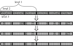
Figure 2: Illustration of the sequence of actions of the $\mathcal{T}_{(1,2,2)}(\cdot)$ operator (as described in Algorithm 2) on a three-level block vector in $\mathbb{C}^{2\cdot 3\cdot 5}$ ($2$ blocks of $3$ blocks of $5$ elements each). The support of the best $(1,2,2)$-Hi-sparse approximation of the vector is $\{1,4,10,13\}$, with index $0$ corresponding to the leftmost element in the vector. Note that this support is different from the support $\{1,9,19,24\}$ of the best $1\times 2\times 2=4$-sparse approximation, when the vector is treated as an arbitrary vector (no block structure) in $\mathbb{C}^{30}$.

It is noted that the notion of hierarchical sparsity is more general than that of the common block sparsity where a vector of length $N$ is partitioned into $N/d$ blocks of $d$ elements each, with $s<N/d$ of the blocks (and their elements) being non-zero [29]. Note that in this case, the vector can be treated as a two-level block vector in $\mathbb{C}^{\frac{N}{d}\cdot d}$ that is $(s,d)$-Hi-sparse.

It is easy to see that the unknown vector $\mathbf{x}$ in (9) is actually a hierarchically sparse, $3$-level block vector under both F-S and S-F options. In particular, under the F-S option and the assumption $LV\leq M$ (reasonable for massive MIMO and sparse channels), $\mathbf{x}\in\mathbb{C}^{M\cdot U\cdot D}$ and is $(LV,V,L)$-Hi-sparse. Note that the first (outer) hierarchy level corresponds to angles (up to $LV$ angle values can be present, equal to the number of total paths from all active UEs), the second hierarchy level corresponds to UEs (up to $V$ active UEs can have a path with the same angle), and the third hierarchy level corresponds to delays (up to $L$ delays per UE per angle can be present, equal to the total paths per UE). However, for (asymptotically) large $M$, one may reasonably assume that (a) for each angle value there can be no more than $K_{V}<V$ UEs with a channel path having this angle and (b) for each angle there can be no more than $K_{L}<L$ paths for each UE with this value, rendering $\mathbf{x}$ as $(LV,K_{V},K_{L})$-Hi-sparse. Under the S-F option, $\mathbf{x}\in\mathbb{C}^{U\cdot D\cdot M}$ and is $(V,L,L)$-Hi-sparse, with the first (outer) hierarchy level corresponding to UEs ($V$ out of $U$ UEs active), the second corresponding to delays (up to $L$ paths present per UE), and the third corresponding to angles (up to $L$ paths with the same delay). Similar to the F-S option, the hierarchical sparsity characterization under S-F option can be refined in the (asymptotically) large $N$ regime, where up to $K_{L}$ paths can be assumed to have the same delay per UE, rendering $\mathbf{x}$ as $(V,L,K_{L})$-Hi-sparse.

The F-S and S-F options result in a different ordering of levels for $\mathbf{x}$ and suggest different (but reasonable) assumptions for the delay/angular distribution of UE channels. However, at this point, it is not clear which of the two options is preferable. Note also that, for asymptotically large $M$ or $N$, it is reasonable to assume that $K_{V}=K_{L}=1$, although we do not explicitly write them as such for generality of presentation.

IV-B Algorithm Design

Clearly, the hierarchically sparse property of $\mathbf{x}$ should be exploited in algorithm design and analysis as it provides significant restrictions on its support, compared to the standard notion of sparsity (which would characterize $\mathbf{x}$ simply as $VL$-sparse). Towards this end, the low-complexity, iterative hard thresholding (IHT) and hard threshold pursuit (HTP) algorithms [20] are modified as shown in Algorithm 1 to take into account the hierarchical sparsity of $\mathbf{x}$ and are referred to in the following as hierarchical IHT (HiIHT) and hierarchical HTP (HiHTP), respectively. The algorithms can be applied equally well under either the F-S or S-F option and are independent of the noise statistics.

Algorithm 1 HiIHT/HiHTP Channel Estimation

0:  $\mathbf{y}$, $\mathbf{A}$, $V$, $L$, $K_{L}$, $K_{V}$ (the latter only under F-S option).

1:  $i=0$, $\hat{\mathbf{x}}^{\left(0\right)}=\mathbf{0}\in\mathbb{C}^{UDM}$

2:  repeat

3:     $i=i+1$,

4:     $\hat{\mathbf{x}}_{\text{temp}}=\hat{\mathbf{x}}^{\left(i-1\right)}+\mathbf{A}^{H}\left({\mathbf{y}}-\mathbf{A}\hat{\mathbf{x}}^{\left(i-1\right)}\right)$

5:     $\hat{\mathcal{S}}^{\left(i\right)}=\begin{cases}\mathcal{T}_{(VL,K_{V},K_{L})}(\hat{\mathbf{x}}_{\text{temp}}),&\text{F-S option,}\\ \mathcal{T}_{(V,L,K_{L})}(\hat{\mathbf{x}}_{\text{temp}}),&\text{S-F option}\end{cases}$

6:     if HiIHT then

7:        $\hat{\mathbf{x}}^{\left(i\right)}=\mathbf{0}\in\mathbb{C}^{UDM}$

8:        $\hat{\mathbf{x}}^{\left(i\right)}_{\hat{\mathcal{S}}^{\left(i\right)}}=\hat{\mathbf{x}}_{\text{temp},\hat{\mathcal{S}}^{\left(i\right)}}$

9:     else if HiHTP then

10:        $\hat{\mathbf{x}}^{\left(i\right)}=\arg\min_{\beta\in\mathbb{C}^{UDM},\text{supp}({\beta})\subseteq\hat{\mathcal{S}}^{\left(i\right)}}\left\{\|\mathbf{y}-\mathbf{A}\beta\|\right\}$

11:     end if

12:  until stopping criterion is met at $i=i^{\ast}$

13:  return  $\begin{cases}(VL,K_{V},K_{L})\text{-Hi-sparse }\hat{\mathbf{x}}^{\left(i^{\ast}\right)},&\text{F-S option,}\\ (V,L,K_{L})\text{-Hi-sparse }\hat{\mathbf{x}}^{\left(i^{\ast}\right)},&\text{S-F option}\end{cases}$

In iteration $i$, the estimate of iteration $i-1$ is first updated by a standard gradient-descent step to obtain $\hat{\mathbf{x}}_{\text{temp}}$. From $\hat{\mathbf{x}}_{\text{temp}}$, the hierarchically sparse support $\mathcal{S}\in[UDM]$ of $\mathbf{x}$ is estimated by application of the thresholding operator $\mathcal{T}_{(\cdot,\cdot,\cdot)}(\cdot)$, to be defined next. For HiIHT, the current iteration estimate of $\mathbf{x}$ is set equal to $\hat{\mathbf{x}}_{\text{temp}}$ except for its elements that do not belong to the estimated support and are set equal to zero. For HiHTP, the iteration $i$ estimate is obtained as the hierarchically sparse vector whose non-zero element values are obtained by minimizing a standard least squares cost function.

Utilization of the operator $\mathcal{T}_{(\cdot,\cdot,\cdot)}(\cdot)$ is the only but critical differentiator of HiIHT/HiHTP compared to their “standard” IHT/HTP counterparts [20]. In particular, for any multi-level block vector $\tilde{\mathbf{x}}\in\mathbb{C}^{N_{1}\cdot N_{2}\cdots N_{\ell}}$ and any $\mathbf{s}=(s_{1},s_{2},\ldots,s_{\ell})$, $\mathcal{T}_{\mathbf{s}}(\tilde{\mathbf{x}})$ is defined as the support of the multi-level block vector $\tilde{\mathbf{z}}\in\mathbb{C}^{N_{1}\cdot N_{2}\cdots N_{\ell}}$ that is $\mathbf{s}$-Hi-sparse and minimizes $\|\tilde{\mathbf{x}}-\tilde{\mathbf{z}}\|$. Its action can be computed recursively with minimal complexity as described in Algorithm 2 with an example of this computation shown in Fig. 2. For the channel estimation problem, $\ell=3$ in the description of the algorithm, with $(N_{1},N_{2},N_{3})=(M,U,D)$ and $(N_{1},N_{2},N_{3})=(U,D,M)$ under the F-S and S-F option respectively.

Algorithm 2 Action of operator $\mathcal{T}_{\mathbf{s}}(\cdot)$

0:  $\tilde{\mathbf{x}}\in\mathbb{C}^{N_{1}\cdot N_{2}\cdots N_{\ell}}$, $\mathbf{s}=(s_{1},s_{2},\ldots,s_{\ell})$, $\ell\geq 2$

1:  $\tilde{\mathbf{z}}=\tilde{\mathbf{x}}$.

2:  For each of the $N_{1}N_{2}\cdots N_{\ell-1}$ blocks at level $\ell-1$ of $\tilde{\mathbf{z}}$, identify the $s_{\ell}$ (out of a total $N_{\ell}$) largest-modulus elements and set the remaining elements equal to zero. Ties are resolved arbitrarily.

3:  $k=\ell-2$ .

4:  while $k\geq 1$ do

5:     For each of the $N_{1}N_{2}\cdots N_{k}$ blocks at level $k$ of $\tilde{\mathbf{z}}$, identify the $s_{k+1}$ (out of a total $N_{k+1}$) blocks with the largest Euclidean norm and set the elements of the remaining blocks equal to zero. Ties are resolved arbitrarily.

6:     $k=k-1$

7:  end while

8:  return  $\text{supp}(\tilde{\mathbf{z}})$

IV-C Performance Analysis and Overhead Requirements

Towards characterizing the performance of HiIHT/HiHTP, which, in turn, will provide insights on pilot signature design and overhead requirements, the concept of hierarchical RIP (HiRIP) constant, first introduced in [27], is essential.

Definition 4 (HiRIP constant).

Let $\mathbf{s}=(s_{1},s_{2},\ldots,s_{\ell})$ be an $\ell$-tuple of natural numbers. The $\mathbf{s}$-HiRIP constant $\delta_{\mathbf{s}}(\tilde{\mathbf{A}})$ of a (deterministic) matrix $\tilde{\mathbf{A}}\in\mathbb{C}^{N_{0}\times(N_{1}N_{2}\cdots N_{\ell})}$ is the smallest $\delta\geq 0$ such that

$$(1-\delta)\|\tilde{\mathbf{x}}\|^{2}\leq\|\tilde{\mathbf{A}}\tilde{\mathbf{x}}\|^{2}\leq(1+\delta)\|\tilde{\mathbf{x}}\|^{2},$$ (13)

for all $\mathbf{s}$-Hi-sparse $\ell$-level block vectors $\tilde{\mathbf{x}}\in\mathbb{C}^{N_{1}\cdot N_{2}\cdots N_{\ell}}$. We say that $\tilde{\mathbf{A}}$ satisfies the $\mathbf{s}$-HiRIP if $\delta_{\mathbf{s}}(\tilde{\mathbf{A}})<\bar{\delta}$ where $\bar{\delta}<1$ is a pre-specified constant.

Remark 5.

The definition of the $\mathbf{s}$-HiRIP constant closely follows Def. 1 of the (standard) $s$-RIP constant and they actually coincide when $\mathbf{s}$ contains only a single element, i.e., it is a scalar. However, when $\mathbf{s}$ is a vector of two or more elements, the notion of HiRIP constant is not directly comparable to that of the RIP constant as the first applies to hierarchically sparse vectors whereas the second applies to more general, sparse vectors (that may or may not be hierarchically sparse). However, a link between the two notions exists by noting that, for any matrix $\tilde{\mathbf{A}}$, it must hold (see Appendix A)

$$\delta_{(s_{1},s_{2},\ldots,s_{\ell})}(\tilde{\mathbf{A}})\leq\delta_{s_{1}s_{2}\cdots s_{\ell}}(\tilde{\mathbf{A}}),$$ (14)

for any $s_{1},s_{2},\ldots,s_{\ell}$, a result that will be utilized in the following.

The HiRIP framework allows to obtain the following rigorous guarantees for the performance of HiIHT/HiHTP.

Theorem 6 (Recovery guarantee of HiIHT/HiHTP).

Assume that $M,N,D\gg L$ and suppose that the sensing matrix $\mathbf{A}$ in (9) has a HiRIP constant

$$\delta\triangleq\begin{cases}\delta_{(3LV,3K_{V},3K_{L})}(\mathbf{A}),&\mathcal{\text{\emph{under F-S option}}},\\ \delta_{(3V,3L,3K_{L})}(\mathbf{A}),&\mathcal{\text{\emph{under S-F option,}}}\end{cases}$$

with

$$\delta<1/\sqrt{3}.$$ (15)

Then, the sequence of estimates $\{\hat{\mathbf{x}}^{\left(i\right)}\}$ generated by the HiIHT and HiHTP algorithms satisfies

$$\|\mathbf{x}-\hat{\mathbf{x}}^{\left(i\right)}\|\leq\kappa^{i}\|\mathbf{x}\|+\tau\|\mathbf{z}\|,$$

for all $i\geq 0$, with

$$\kappa\triangleq\begin{cases}\sqrt{3}\delta,&\text{\emph{for HiIHT},}\\ \sqrt{2\delta/(1-\delta^{2})},&\text{\emph{for HiHTP},}\end{cases}$$

and

$$\tau\triangleq\begin{cases}2.18/(1-\kappa),&\text{\emph{for HiIHT}},\\ 5.15/(1-\kappa),&\emph{for HiHTP}.\end{cases}$$

Proof:

The result for the HiHTP follows directly from application of [27, Theorem 4]. The proof for the HiIHT follows the HiHTP proof with the same modifications as the ones considered in the recovery guarantee proofs of the HTP/IHT algorithms given in [20, Theorem 6.18]. ∎

It follows that in order to ensure reliable channel estimation in the sense of perfect and bounded-error recovery of $\mathbf{x}$ via the HiHTP/HiIHT algorithms in the noiseless ($\|\mathbf{z}\|=0$) and noisy ($\|\mathbf{z}\|>0$) case, respectively, we need to design $\mathcal{N}_{p}$, $\mathcal{M}_{p}$, and $\{\mathbf{c}_{u}\}_{u=0}^{U-1}$ such that the HiRIP constant of $\mathbf{A}$ satisfies (15). Similar to RIP, the explicit computation of HiRIP constants is a very difficult problem (even numerically) [28]. However, the following bound on the HiRIP constant of a Kronecker-product sensing matrix in terms of the RIP constants of its factor matrices is available, which can be used to obtain a rigorous description of the overhead required to achieve (15).

Lemma 7.

Consider a matrix $\tilde{\mathbf{A}}\triangleq\tilde{\mathbf{A}}_{1}\otimes\tilde{\mathbf{A}}_{2}$, with $\tilde{\mathbf{A}}_{k}\in\mathbb{C}^{M_{k}\times N_{k}},k=1,2$, which, for all $3$-level block vectors $\tilde{\mathbf{x}}\in\mathbb{C}^{N^{\prime}_{1}\cdot N_{2}^{\prime}\cdot N_{3}^{\prime}}$ with $N_{1}^{\prime}N_{2}^{\prime}N_{3}^{\prime}=N_{1}N_{2}$, has an $\mathbf{s}$-HiRIP constant $\delta_{\mathbf{s}}(\tilde{\mathbf{A}})$ for some $\mathbf{s}\triangleq(s_{1},s_{2},s_{3})$. If $N_{1}=N_{1}^{\prime}$ and $N_{2}=N_{2}^{\prime}N_{3}^{\prime}$, it holds

$$\delta_{\mathbf{s}}(\tilde{\mathbf{A}})\leq\left(1+\delta_{s_{1}}(\tilde{\mathbf{A}}_{1})\right)\left(1+\delta_{s_{2}s_{3}}(\tilde{\mathbf{A}}_{2})\right)-1,$$ (16)

whereas, if $N_{1}=N_{1}^{\prime}N_{2}^{\prime}$ and $N_{2}=N_{3}^{\prime}$, it holds

$$\delta_{\mathbf{s}}(\tilde{\mathbf{A}})\leq\left(1+\delta_{s_{1}s_{2}}(\tilde{\mathbf{A}}_{1})\right)\left(1+\delta_{s_{3}}(\tilde{\mathbf{A}}_{2})\right)-1.$$ (17)

Proof:

The bound of (16) follows from the inequality [28, Theorem 4]

$$\delta_{\mathbf{s}}(\tilde{\mathbf{A}})\leq\left(1+\delta_{s_{1}}(\tilde{\mathbf{A}}_{1})\right)\left(1+\delta_{(s_{2},s_{3})}(\tilde{\mathbf{A}}_{2})\right)-1,$$

and (14). The bound of (17) follows by the inequality

$$\delta_{\mathbf{s}}(\tilde{\mathbf{A}})\leq\left(1+\delta_{(s_{1},s_{2})}(\tilde{\mathbf{A}}_{1})\right)\left(1+\delta_{s_{3}}(\tilde{\mathbf{A}}_{2})\right)-1,$$

which can be shown to hold by a straightforward extension of the proof of [28, Theorem 4] and again applying (14). ∎

The importance of this theorem is that it bounds the HiRIP constant of $\mathbf{A}$ in terms of the RIP constants of its constituent matrices $\bar{\mathbf{A}}_{\tau}$ and $\bar{\mathbf{A}}_{\theta}^{*}$. Any design resulting in this bound of the HiRIP constant of $\mathbf{A}$ been less than $1/\sqrt{3}$ is therefore sufficient to achieve the performance guarantees of Theorem 6. To this end, we propose the following design.

Definition 8 (System Design).

Set $U\leq N/D$ and let $\mathbf{c}\in\mathbb{C}^{N}$ be an arbitrary sequence of unit modulus elements. For an arbitrary group of $U$ UEs, the set of its dedicated pilot subcarriers $\mathcal{N}_{p}$ is a randomly and uniformly selected subset of $[N]$ with cardinality $N_{p}$, whereas the set of observed antennas $\mathcal{M}_{p}$ is randomly and uniformly selected subset of $[M]$ with cardinality $M_{p}$ (same for all UE groups). The UE signature sequences are

$$\mathbf{c}_{u}=\mathbf{P}_{\mathcal{N}_{p}}\text{diag}\left(\left[1,e^{-j\frac{2\pi}{N}uD},\ldots,e^{-j\frac{2\pi}{N}uD(N-1)}\right]\right)\mathbf{c},$$ (18)

for all $u\in[U].$

Note that under this design the joint assignment of pilot subcarriers to multiple UE groups is simplified to a random partition of subcarriers. This design is motivated by the availability of rigorous RIP constant characterization for matrices obtained by random sampling of rows of orthogonal matrices. Indeed, it immediately follows from (8) and the random selection of antennas that $\bar{\mathbf{A}}_{\theta}^{*}$ is a random sampling of the rows of the orthogonal matrix $(1/\sqrt{M_{p}})\mathbf{F}_{M,M}^{*}$, whereas, direct substitution of (18) into (7) results in

$$\mathbf{\bar{A}}_{\tau}=(1/\sqrt{N_{p}})\mathbf{P}_{\mathcal{N}_{p}}\text{diag}(\mathbf{c})\mathbf{F}_{N,UD},$$ (19)

i.e., $\mathbf{\bar{A}}_{\tau}$ is a random sampling of the rows from the first $UD$ columns of the orthogonal matrix $(1/\sqrt{N_{p}})\text{diag}(\mathbf{c})\mathbf{F}_{N,N}$. Equally important, this form of $\bar{\mathbf{A}}_{\theta}^{*}$ and $\bar{\mathbf{A}}_{\tau}$ allows for the efficient computation of the gradient-descent step in Algorithm 1 by means of fast Fourier transform (FFT). This makes HiIHT in particular especially attractive for application in systems with (very) large $M$ and/or $N$. We note that phase-shifted pilot sequence designs similar to (18) were also proposed in [7, 17, 30], however, under different contexts in terms of system model and/or assuming regularly-spaced pilot subcarriers. In addition, the well-known Zadoff-Chu sequences employed in cellular standards [31] are compatible with the design of (18).

The proposed design cannot be claimed to be optimal in the sense that it is not obtained as the explicit solution of an optimization problem. However, as will be shown in Sec. VI, it achieves very good performance and, equally important, results in a sensing matrix $\mathbf{A}$ whose HiRIP can be analytically characterized as a function of $N_{p}$ and $M_{p}$. This characterization, in combination with the performance guarantees of Theorem 6, allows for rigorous analytical insights on the overhead requirements for reliable channel estimation, as stated in the following result.

Theorem 9.

Let $\delta_{\tau}>0$, $\delta_{\theta}>0$ be two arbitrary numbers that satisfy $\delta_{\tau}+\delta_{\theta}+\delta_{\tau}\delta_{\theta}<1/\sqrt{3}$. With the proposed design and with a probability greater than $1-M^{-\log^{3}(M)}-N^{-\log^{3}(N)}$, the HiIHT/HiHTP algorithm performance is as described in Theorem 6 when it holds

$$N_{p} \geq\min\left\{3C\delta_{\tau}^{-2}K_{V}K_{L}\log^{4}(N),N\right\},$$ (20)

$$M_{p} \geq\min\left\{9C\delta_{\theta}^{-2}VL\log^{4}(M),M\right\},$$ (21)

under the F-S option, or

$$N_{p} \geq\min\left\{9C\delta_{\tau}^{-2}VL\log^{4}(N),N\right\},$$ (22)

$$M_{p} \geq\min\left\{3C\delta_{\theta}^{-2}K_{L}\log^{4}(M),M\right\},$$ (23)

under the S-F option, where $C>0$ is a universal constant.

Proof:

Please see Appendix B. ∎

The following remarks are in order:

• Both F-S and S-F options require an overhead $N_{p}M_{p}$ that is proportional to $VL$ (assuming $M,N\gg L$ and $K_{V},K_{L}$ independent of $V$ and $L$), similarly to the universal bound of (12). Of course, using $N_{p}=N$ and $M_{p}=M$ will result in the best performance in the presence of noise, however, this would be achieved with an overly large overhead cost.

• There is flexibility in distributing the overhead over the frequency and space dimensions by changing the values of $\delta_{\tau}$ and $\delta_{\theta}$ in Theorem 9. The minimum pilot overhead ($N_{p}$) is achieved with $\delta_{\theta}=\epsilon$ and $\delta_{\tau}=1/\sqrt{3}-\epsilon$, for some arbitrarily small $\epsilon>0$, resulting in $M_{p}=M$, i.e., all antennas are utilized, whereas minimum number of observed antennas is achieved with $\delta_{\tau}=\epsilon$ and $\delta_{\theta}=1/\sqrt{3}-\epsilon$ with all subcarriers utilized for training.

• The scaling laws for $N_{p}$ and $M_{p}$ are different between the F-S and S-F option due to the different hierarchical sparsity properties for $\mathbf{x}$ corresponding to each of these (see discussion in Sec. IV. A). Interestingly, under the F-S option and assuming that $K_{V}$ and $K_{L}$ are independent of $V$ and $L$, $N_{p}$ is independent of the number of channel paths $L$ and active UEs $V$, which is particularly appealing as it implies a robust pilot design without a need for pilot reconfiguration with changing $L$ and/or $V$. Of course, one expects that performance will degrade with increasing $L$ and/or $V$ with a fixed $N_{p}$, however, as long as (21) holds, this degradation is expected to be graceful in the sense of achieving a bounded estimation error, as also verified in the numerical results of Sec. VI. Similar conclusions hold for the S-F option, this time with $M_{p}$ being independent of $L$ and $V$.

• The result of Theorem 9, even though only sufficient, provides a much better indication of the minimum possible overhead requirements than the one provided by conventional (unstructured) CS theory. Indeed, under the conventional CS treatment, a sufficient condition to achieve reliable channel estimation is $\delta_{cVL}(\mathbf{A})<\delta_{\text{RIP}}$, where the values of $c>0$ and $\delta_{\text{RIP}}>0$ depend on the considered estimation algorithm [20]. For Kronecker-type sensing matrices $\tilde{\mathbf{A}}=\tilde{\mathbf{A}}_{1}\otimes\tilde{\mathbf{A}}_{2}$, it is known that $\delta_{s}(\tilde{\mathbf{A}})\geq\max\{\delta_{s}(\mathbf{A}_{1}),\delta_{s}(\mathbf{A}_{2})\}$, for any $s$ [21, 22], which for the massive MIMO channel estimation problem implies that the pilot design should be such that it holds $\delta_{cVL}(\mathbf{A}_{\tau})<\delta_{\text{RIP}}$ and $\delta_{cVL}(\mathbf{A}_{\theta})<\delta_{\text{RIP}}$. For the training sequence design considered above, it is easy to show that in order to achieve this condition both $N_{p}$ and $M_{p}$ should scale proportionally to $VL$ (up to logarithmic factors), irrespective of $c$ and $\delta_{\text{RIP}}$. In contrast, Theorem 9 reveals that only one of $N_{p}$ and $M_{p}$ needs to scale proportionally to $VL$ (up to logarithmic factors).

• The overhead requirement of Theorem 9 is a sufficient condition for the application of the HiIHT/HiHTP algorithms. Therefore, this value may be greater than the necessary and sufficient overhead requirement when a more sophisticated and more complex algorithm such as, e.g., maximum likelihood estimation, is employed.

• The HiIHT/HiHTP algorithm description, performance analysis, and overhead requirements described in this section are independent of the statistics of UE channels as well as noise. The only assumption considered is that each UE channel consists of $L$ paths with on-grid values for angles and delays.

As the pilot overhead reduction is critical towards increasing the system capacity, i.e., accommodate more UEs and/or increase per-UE rates, it is clear that the F-S option is preferable as $N_{p}$ does not scale with $V$ and $L$ (assuming that $K_{V}$ and $K_{L}$ are also independent of $V$, $L$). In particular, we have the following sufficient pilot overhead requirement obtained by setting $\delta_{\theta}=\epsilon$ and $\delta_{\tau}=1/\sqrt{3}-\epsilon$, $\epsilon\rightarrow 0$, in Theorem 9.

Corollary 10.

Towards achieving reliable channel estimation with minimum pilot overhead, the F-S option should be selected with $M_{p}=M$ (full antenna array utilization) and

$$N_{p}\geq CK_{V}K_{L}\log^{4}(N),$$

where $C$ is a universal constant.

It is noted that the independence of the scaling behavior of the pilot overhead from $L$ and $V$ is only possible by the utilization of a massive number of antennas. In a loose sense, under the F-S option, we shift the estimation burden to the spatial domain and corresponding measurements, thus allowing for a minimum overhead in the frequency domain. It is easy to see that when $M=1$, only the S-F option is available, which results in a pilot overhead that scales with $L$ and $V$.

V Extension to Off-Grid Channel Parameters

The previous sections considered on-grid channel parameters, which can be assumed to be a good approximation in the regime of asymptotically large $M$ and $N$. The fundamental benefit offered by this assumption is that it naturally introduces the delay-angular channel representation according to (3) and (4) that is exploited for algorithm development and system design. Considering an arbitrary UE transfer matrix $\mathbf{H}\in\mathbb{C}^{N\times M}$ corresponding to a channel with off-grid parameters, a unique delay-angular channel representation as in (3) exists only by treating the delay spread as equal to the OFDM symbol duration $T_{s}$, i.e., $D=N$, even if the actual spread is actually smaller than this value. Under this assumption, it follows from (2) and (3) that the delay-angular representation equals

$$\mathbf{X} =\mathbf{F}_{N,N}^{-1}\mathbf{H}(\mathbf{F}_{M,M}^{H})^{-1}.$$ (24)

An example of $\mathbf{X}$ for a channel with off-grid parameters is shown in Fig. 1 (right panel). It can be seen that, in contrast to the on-grid case, the energy of each path is leaked over all elements of $\mathbf{X}$ rendering it non-sparse. However, most of the energy of each path is concentrated on a few elements of $\mathbf{X}$, suggesting that the latter can be approximated by a sparse matrix, which, as in the on-grid case, can be exploited in the channel estimation procedure. This approximate sparsity of $\mathbf{X}$ in the off-grid case is confirmed by the following result.

Theorem 11.

Let $L_{1}\leq\frac{N-1}{2}$, $L_{2}\leq\frac{M-1}{2}$ be strictly positive integers. Setting $D=N$, the delay-angle representation $\mathbf{X}\in\mathbb{C}^{N\times M}$ of any channel with $L$ paths of arbitrary (off-grid) delay and angle values can be approximated by a sparse matrix $\mathbf{X}_{\text{\emph{sp}}}\in\mathbb{C}^{N\times M}$ that consists of at most $L(2L_{1}+1)(2L_{2}+1)$ non zero elements with an error

$$\left\|\mathbf{X}-\mathbf{X}_{\text{\emph{sp}}}\right\|\leq\left(\frac{1}{\sqrt{L_{1}}}+\frac{1}{\sqrt{L_{2}}}\right)\sum_{p=0}^{L-1}\left|\rho_{p}\right|,$$ (25)

where $\rho_{p}$ is the complex gain of the $p$-th channel path.

Proof:

Please see Appendix C. ∎

The result implies that by choosing the parameters $L_{1}$ and $L_{2}$ sufficiently large, the delay-angular representation of any channel with $L$ off-grid paths can be approximated with small error by the delay-angular representation of a channel with $L(2L_{1}+1)(2L_{2}+1)$ on-grid paths. This increase of on-grid equivalent paths is due to the, so called, basis mismatch error [32] and can be viewed as the cost of representing the channel on the fixed basis corresponding to the dictionary matrices $\mathbf{A}_{\tau}$, $\mathbf{A}_{\theta}$.

Since an accurate on-grid representation is available, the HiIHT/HiHTP algorithms operating under the on-grid assumption can be employed to identify the $L(2L_{1}+1)(2L_{2}+1)$ equivalent on-grid paths per UE. In particular, the proof of Theorem 11 considers a delay-angular representation where most of each path energy spills over $L_{1}$ consecutive on-grid delay values and $L_{2}$ consecutive on-grid delay values. The example of Fig. 1 identifies these energy regions for each path assuming $L_{1}=L_{2}=1$. By the same arguments discussed in the on-grid case and considering the F-S option, the sparse vector $\mathbf{x}$ to be estimated according to the model (9) by HiIHT/HiHTP is now $(VL(2L_{2}+1),K_{V},K_{L}(2L_{1}+1))$-Hi-sparse in $\mathbb{C}^{M\cdot U\cdot D}$.

Note that this approach will introduce the following four errors compared to the on-grid case discussed in the previous sections: (a) channel representation error due to the consideration of $\mathbf{X}_{\text{sp}}\in\mathbb{C}^{N\times N}$ instead of $\mathbf{X}\in\mathbb{C}^{N\times M}$, as described above, for any UE channel, (b) channel representation error due to the algorithms estimating a $D\times M$ (instead of $N\times M$) delay-angular matrix representation for each UE (implying the “missing” $N-D$ columns are estimated as zeros), (c) channel estimation error due to the channel representation error treated as an additional noise term by the algorithm, and (d) channel estimation error due to the increase of unknown parameters to be estimated. Note that these error terms are controlled to a large extent by the design parameters $L_{1}$ and $L_{2}$. These should be selected to satisfy the two conflicting requirements: reduce the sparse channel representation error (large values for $L_{1}$ and $L_{2}$) and reduce the number of parameters to be estimated (small values for $L_{1}$ and $L_{2}$).

We numerically investigate the performance in the off-grid case and the selection of $L_{1}$, $L_{2}$ in Sec. VI.

VI Numerical Results

For demonstrating the merits of the proposed, hierarchical-sparsity-based framework for channel estimation, numerical examples are presented in this section, demonstrating its effectiveness in achieving good channel estimation accuracy with limited pilot overhead $N_{p}$.

In all cases, an OFDM system with $N=1024$ subcarriers and a BS with a ULA equipped with $M=256$ antennas are considered. Note that, for these system parameters, the channel transfer matrix of each UE consists of $MN=262144$ elements, a huge number that imposes insurmountable computational challenges to conventional estimation approaches in addition to performance and overhead issues. For all UEs, the channel consists of $L$ paths and has a maximum delay spread equal to $1/4$ of the useful OFDM symbol period. The channel path gains for each UE were generated as i.i.d. zero mean, complex Gaussian variables with a total power $\sum_{p=0}^{L-1}\mathbb{E}(|\rho_{p}|^{2})=1$, resulting in an average received power per subcarrier also equal to $1$ for all UEs (note that the pilot signatures of the proposed design consist of unit-modulus symbols). The elements of the noise matrix $\mathbf{Z}$ in (5) were generated as i.i.d. zero mean, complex Gaussian random variables of variance $1/\mathsf{SNR}$, where $\mathsf{SNR}$ denotes the average received signal-to-noise ratio per subcarrier.

Towards minimizing the pilot overhead, the F-S option will be considered throughout with $M_{p}=M$, i.e., all antenna signals are used, unless stated otherwise. In most examples, the HiIHT algorithm is employed due to its simple implementation. The iterations of HiIHT and HiHTP terminate when the estimated support between two consecutive iterations remains the same or when ten iterations have been performed.

VI-A The On-Grid Case

Single User Case: The single-UE case is considered first (i.e., $U=V=1$). The path angles $\{\theta_{p}\}_{p=0}^{L-1}$ are generated independently and uniformly over the angle sampling grid determined by $\mathbf{A}_{\theta}$, however, no two paths are allowed to have the same angle, which is a reasonable assumption for the asymptotic $M$ case. The path delays $\{\tau_{p}\}_{p=0}^{L-1}$ are generated independently and uniformly over the delay sampling grid determined by $\mathbf{A}_{\tau}$ with $D=N/4=256$. Note that this channel model corresponds to an $(L,1,1)$-Hi-sparse vector $\mathbf{x}\in\mathbb{C}^{M\cdot U\cdot D}$ in (9).

Figure 3 depicts the per-element mean squared error (MSE) $\frac{1}{NM}\mathbb{E}(\|\mathbf{H}-\hat{\mathbf{H}}\|^{2})$ of the channel matrix estimate $\hat{\mathbf{H}}\triangleq\mathbf{A}_{\tau}\mathbf{\hat{X}}\mathbf{A}_{\theta}^{H}$, where $\hat{\mathbf{X}}$ is the estimate of the delay-angular channel representation provided by HiIHT, as a function of the normalized pilot overhead $N_{p}/N$ and for various values of $L$ (assumed known at the BS). The $\mathsf{SNR}$ was set equal to 10 dB.

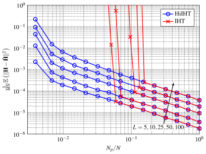
Figure 3: Single UE MSE of HiIHT and IHT estimators as a function of pilot overhead (on-grid case, $N=1024,M=256,D=256,\mathrm{\mathsf{SNR}}=10\text{ dB}$).

It can be seen that HiIHT offers excellent estimation accuracy with a very small pilot overhead. For example, a normalized pilot overhead of around $10^{-2}$ is sufficient to achieve a MSE that is at least one order of magnitude less than the noise variance level $1/\mathsf{SNR}=10^{-1}$, which corresponds to the MSE achieved with $N_{p}=N$ and the naive channel estimate $\hat{\mathbf{H}}=\mathbf{Y}$. This pilot overhead should be compared with conventional (non sparsity-exploiting) estimation approaches which would require a normalized pilot overhead approximately $D/N=0.25$ [36] (see also discussion of Fig. 7). As expected, the performance of HiIHT degrades with increasing $L$ as the number of unknown parameters increases. However, note that (a) this degradation is rather graceful, i.e., the MSE remains bounded, and (b) the minimum required overhead to achieve a bounded MSE is independent of $L$, in line with the remarks made in the discussion of Theorem 9. Note also that reasonable MSE is also achieved even with $L>N_{p}$. This reflects the advantage of observing multiple antennas and is in line with the flexibility in distributing overhead indicated by Theorem 9. Of course, in the single antenna case ($M=1$), reliable channel estimation can only be achieved with $N_{p}\geq L$.

As a comparison, the performance of the standard IHT algorithm is depicted in Fig. 3. A “phase transition” phenomenon is clearly seen: a minimum pilot overhead is required in order to achieve a reasonable MSE performance that is at least $6$ times greater than the one needed by HiIHT to achieve a MSE less than $10^{-2}$. Also, this minimum overhead is increasing with $L$. This clearly demonstrates the advantage of exploiting the hierarchical channel sparsity in the channel estimation procedure, which allows for reliable and robust performance in the small pilot overhead regime. For sufficiently large training overhead, the performances of IHT and HiIHT are the same, implying that knowledge of the sparsity structure plays no role in this regime. This is in line to the well-known fact from estimation theory that a priori information (in this case, hierarchical structure of sparsity) becomes irrelevant once sufficiently many observations have been obtained.

Multiuser Case: The multiuser case is considered next. Note that for the scenario with $D=N/4$ considered here, up to $U=4$ UEs can be supported per UE group by the pilot sequence assignment scheme of Sec. IV. With $\mathsf{SNR}=10$ dB and UE channels with $L=3$ paths generated independently as described in the single UE case example, Fig. 4 demonstrates the total MSE, defined as $\frac{1}{MN}\sum_{u=0}^{U-1}\mathbb{E}(\|\mathbf{H}_{u}-\hat{\mathbf{H}}_{u}\|^{2})$, for various number of randomly and uniformly selected active UEs $V\leq U$. Note that, in the MSE formula, $\mathbf{H}_{u}$ is equal to zero if the UE is not active.

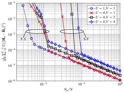
Figure 4: Multiuser MSE of HiIHT estimator as a function of pilot overhead (on-grid case, $N=1024,M=256,D=256,L=3,\mathrm{\mathsf{SNR}}=10\text{ dB}$).

When only one UE is active, i.e., $V=1$, a slightly larger pilot overhead compared to the single UE case ($U=V=1)$ is required to achieve the same MSE performance. This overhead cost can be attributed to the uncertainty at the BS of who the actual active UE is. By increasing $V$, a degradation of MSE performance is observed that is proportional to $V$ due to the corresponding increase of unknown parameters to be estimated. However, the minimum required overhead to achieve a bounded channel estimation error is independent of $V$, as guaranteed by Theorem 9.

Figure 4 also depicts the MSE performance under the S-F option. For this case, the channel vector $\mathbf{x}$ in (9) was generated as an $(V,L,1)$-Hi-sparce vector in $\mathbb{C}^{U\cdot D\cdot M}$ with path gains having the same statistics as in the channel model considered under the F-S option. It can be seen that this approach (a) requires increased training overhead to achieve reliable channel estimation and (b) the minimum overhead increases with $V$. Both these observations are consistent with Theorem 9.

Unknown $L$: Both the analysis and the previous results assume knowledge of the number of channel paths $L$. Figure 5 shows the performance of HiIHT assuming $\hat{L}$ number of paths instead of $L$. A case with $U=4,V=2$, and $N_{p}=15$ pilot subcarriers is considered with the rest of the system parameters same as above. As expected, there is degradation in MSE when $\hat{L}\neq L$. This degradation is much more prominent when $\hat{L}<L$, whereas $\hat{L}>L$ results in a moderate degradation. This suggests that setting $\hat{L}$ as an upper bound (worst case) value could be a practical approach when $L$ is unknown. Another approach is to modify HiIHT/HiHTP so as it also provides an estimate of $L$, as described in, e.g., [33, 34].

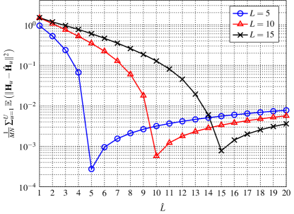
Figure 5: Performance of HiIHT under mismatched $L$ ($N=1024,M=256,D=256,N_{p}=15,U=4,V=2,\mathsf{SNR}=10\text{ dB}$).

Comparison with Orthogonal Matching Pursuit (OMP): In this example, we compare the proposed HiIHT/HiHTP algorithms with the commonly employed OMP algorithm [20], which forms the basis for many previously proposed massive MIMO channel estimation schemes [18, 23]. OMP is a greedy, iterative algorithm of roughly the same complexity as HiHTP. It ignores any structural properties of sparsity, i.e., treats the unknown vector in (9) as $VL$-sparse, instead of $(VL,1,1)$-Hi-sparse (the F-S option is considered). Simulations (not shown here) with $M_{p}=M$ showed that OMP achieved the exact same performance as HiIHT and HiHTP. Towards identifying performane differences, we considered a case with $M_{p}=M/4=64$, with the remaining system parameters same as above and the results are shown in Fig. 6. It can be seen that, in this scenario, OMP is a competitive alternative of HiHTP, whereas HiIHT performs slightly worse but is significantly less complex. The good performance of OMP in estimating hierarchically sparse vectors, even though not explicitly taking this property into account, was previously identified analyzed in [35]. This close correspondence of OMP with HiHTP/HiIHT suggests that the analytical results in this paper may have broader applicability than the HiHTP/HiIHT algorithms. We leave this topic for future investigation.

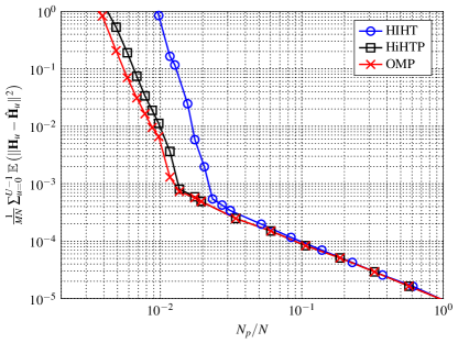
Figure 6: Performance comparison of HiHTP, HiIHT, and OMP ($N=1024,M=256,D=256,L=3,M_{p}=64,U=4,V=2,\mathsf{SNR}=10\text{ dB}$).

VI-B The Off-Grid case

Figure 7 demonstrates the single UE MSE performance for the off-grid case, where the channel is generated as described in the on-grid case with $L=3$, however, with the paths angles and delays uniformly and independently distributed over the continuous domains $[0,1)$ and $[0,T_{S}/4)$, respectively. The $\mathsf{SNR}$ was set to $10$ dB.

As can be seen, performance of HiIHT strongly depends on the choice of $L_{1}$ and $L_{2}$. Small values of these parameters result in the estimation of a small number of unknown parameters by the channel estimator, however, with the cost of a large sparse channel approximation error. As can be seen, the optimal values of $L_{1}$, $L_{2}$ are proportional to the pilot overhead, which is expected as increasing the latter allows for the reliable estimation of more parameters. In any case, the basis mismatch effect results in a great performance degradation compared to the idealized, on-grid examples presented above. However, a MSE of almost an order of magnitude less that the noise level is achievable, rendering the effect of the channel estimation error negligible at the decoding stage.

For comparison, the performance of the conventional, linear minimum mean squares estimator (LMMSE) estimator with equally-spaced pilot subcarriers is depicted in Fig. 7. The LMMMSE estimator utilizes only information about the correlation function $\mathbb{E}([\mathbf{H}]_{n,m}[\mathbf{H}]_{n^{\prime},m^{\prime}}^{*})$ for $n,n^{\prime}\in[N]$, $m,m^{\prime}\in[M]$. The latter can be obtained by a straightforward generalization of the approach shown in [36] for the single receive antenna case. It can be seen that the LMMSE estimator performs very poorly, requiring at least $N_{p}/N\approx 0.25$ in order to achieve an MSE that is equal to the noise level. This is due to the correlation function not capturing the sparsity properties of the channel. Figure 7 also shows the performance of the standard IHT algorithm operating assuming $LK_{\tau}K_{\theta}$ on-grid paths, i.e., the same number of on-grid paths considered by HiIHT. It can be seen that IHT provides a reasonable performance only for large pilot overhead (greater than $0.4$). In that regime, it actually provides a better MSE than HiIHT suggesting that the hierarchical sparsity structure assumed by the HiIHT is not accurate, resulting in an additional error term introduced in the estimate due to this mismatch. However, even though not accurate the assumption of hierarchical sparsity is beneficial in the small pilot overhead regime.

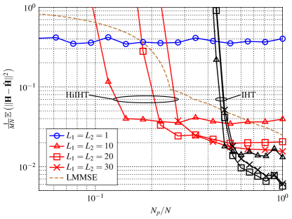
Figure 7: Single UE MSE of HiHTP, HTP and LMMSE estimators as a function of pilot overhead (off-grid case, $N=1024,M=256,D=256,\mathrm{SNR}=10\text{ dB}$).

VII Conclusion

The problem of channel estimation for multiuser wideband massive MIMO via a compressive sensing approach was investigated. Under the assumption of on-grid channel param- eters, a problem reformulation that highlights the hierarchical sparsity property of the wireless channel was considered. This property was taken into account for the design of low- complexity channel estimation algorithms. Using the HiRIP analysis framework, rigorous performance guarantees for these algorithms were obtained that, in turn, provide design rules for UE pilot signature design and selection of pilot subcarriers. A characterization of the sufficient pilot overhead required to achieve reliable channel estimation was provided, revealing that in the massive MIMO regime, the number of subcarriers is independent from the number of active UEs and channel paths per UE. These observations were also verified numerically, with the proposed algorithm showing significant performance gain over conventional CS approaches of similar complexity. Application of the algorithms in a multiple measurements and off-grid channel parameter setting was discussed. For the later case, which is valid in the finite antenna and bandwidth regime, even though there exists an error due to model mismatch, performance of proposed algorithms is still significantly better from conventional CS as well as the standard LMMSE approach.

Appendix A Proof of (14)

Let $\{(N_{i},s_{i})\}_{i=1}^{\ell}$ be a set of $\ell$ tuples of integers such that $N_{i}\geq s_{i}\geq 1$ for all $i$. Denote $\mathcal{S}_{(s_{1},s_{2},\ldots,s_{\ell})}\subseteq\mathbb{C}^{N_{1}\cdot N_{2}\cdots N_{\ell}}$ the set of all $(s_{1},s_{2},\ldots,s_{\ell})$-Hi-sparse vectors in $\mathbb{C}^{N_{1}\cdot N2\cdots N_{\ell}}$, and $\mathcal{S}_{s_{1}s_{2}\cdots s_{\ell}}\subseteq\mathbb{C}^{N_{1}N_{2}\cdots N_{\ell}}$ the set of all $s_{1}s_{2}\cdots s_{\ell}$-sparse vectors in $\mathbb{C}^{N_{1}N2\cdots N_{\ell}}$. Note that $\mathcal{S}_{(s_{1}s_{2}\cdots s_{\ell})}\subseteq\mathcal{S}_{s_{1}s_{2}\cdots s_{\ell}}$. For an arbitrary matrix $\tilde{\mathbf{A}}\in\mathbb{C}^{N_{0}\times(N_{1}N_{2}\cdots N_{\ell})}$, $N_{0}\geq 1$, it follows from the definition of the HiRIP and RIP constants that

$$\delta_{(s_{1},s_{2},\ldots,s_{\ell})}(\tilde{\mathbf{A}}) =\underset{\mathbf{x}\in\mathcal{S}_{(s_{1},s_{2},\ldots,s_{\ell})}}{\max}\frac{\left|\|\tilde{\mathbf{A}}\mathbf{x}\|^{2}-\|\mathbf{x}\|^{2}\right|}{\|\mathbf{x}\|^{2}}$$

$$\leq\underset{\mathbf{x}\in\mathcal{S}_{s_{1}s_{2}\cdots s_{\ell}}}{\max}\frac{\left|\|\tilde{\mathbf{A}}\mathbf{x}\|^{2}-\|\mathbf{x}\|^{2}\right|}{\|\mathbf{x}\|^{2}}$$

$$=\delta_{s_{1}s_{2}\cdots,s_{\ell}}(\tilde{\mathbf{A}}).$$

Appendix B Proof of Theorem 9

Let $\tilde{\mathbf{x}}\neq\mathbf{0}\in\mathbb{C}^{UD}$ denote the $s$-sparse vector for which $\left|\|\bar{\mathbf{A}}_{\tau}\tilde{\mathbf{x}}\|^{2}-\|\tilde{\mathbf{x}}\|^{2}\right|=\delta_{s}(\bar{\mathbf{A}}_{\tau})\|\tilde{\mathbf{x}}\|^{2}$, where $\delta_{s}(\bar{\mathbf{A}}_{\tau})$ is the $s$-RIP constant of matrix $\bar{\mathbf{A}}_{\tau}$ given in (19). Let $\tilde{\mathbf{x}}_{\text{ext}}\triangleq[\tilde{\mathbf{x}}^{T},\mathbf{0}^{T}]^{T}\in\mathbb{C}^{N}$ denote its zero padded extension that is also $s$-sparse. Consider $\bar{\mathbf{A}}_{\tau,\text{ext}}\triangleq(1/\sqrt{N_{p}})\mathbf{P}_{\mathcal{N}_{p}}\text{diag}(\mathbf{c})\mathbf{F}_{N,N}$. It holds

$$\delta_{s}(\bar{\mathbf{A}}_{\tau})\|\tilde{\mathbf{x}}\|^{2} =\left|\|\bar{\mathbf{A}}_{\tau}\tilde{\mathbf{x}}\|^{2}-\|\tilde{\mathbf{x}}\|^{2}\right|$$

$$=\left|\|\bar{\mathbf{A}}_{\tau,\text{ext}}\tilde{\mathbf{x}}_{\text{ext}}\|^{2}-\|\tilde{\mathbf{x}}_{\text{ext}}\|^{2}\right|$$

$$\leq\underset{s\text{-sparse }\mathbf{p}\in\mathbb{C}^{N},\|\mathbf{p}\|=\|\tilde{\mathbf{x}}\|}{\max}\left|\|\bar{\mathbf{A}}_{\tau,\text{ext}}\mathbf{p}\|^{2}-\|\mathbf{p}\|^{2}\right|$$

$$\leq\delta_{s}(\bar{\mathbf{A}}_{\tau,\text{ext}})\|\tilde{\mathbf{x}}\|^{2},$$

where $\delta_{s}(\bar{\mathbf{A}}_{\tau,\text{ext}})$ is the $s$-RIP constant of matrix $\bar{\mathbf{A}}_{\tau,\text{ext}}$, resulting in

$$\delta_{s}(\bar{\mathbf{A}}_{\tau})\leq\delta_{s}(\bar{\mathbf{A}}_{\tau,\text{ext}}),\text{ for all }s\leq UD.$$ (26)

Now consider the F-S option, i.e., with $\mathbf{A}=\bar{\mathbf{A}}_{\theta}^{*}\otimes\bar{\mathbf{A}}_{\tau}$ acting on $\mathbf{x}\in\mathbb{C}^{M\cdot U\cdot D}$. It holds

$$\delta_{(3VL,3K_{V},3K_{L})}(\mathbf{A})$$

$$\overset{(a)}{\leq} \left(1+\delta_{3VL}\left(\bar{\mathbf{A}}_{\theta}^{*}\right)\right)\left(1+\delta_{9K_{V}K_{L}}\left(\bar{\mathbf{A}}_{\tau}\right)\right)-1$$

$$\overset{(b)}{\leq} \left(1+\delta_{3VL}\left(\bar{\mathbf{A}}_{\theta}^{*}\right)\right)\left(1+\delta_{9K_{V}K_{L}}\left(\bar{\mathbf{A}}_{\tau,\text{ext}}\right)\right)-1,$$

where $(a)$ follows from Theorem 7 and ($b)$ from (26). Therefore, a sufficient condition for (15) to hold is

$$1/\sqrt{3} >\left(1+\delta_{3VL}\left(\bar{\mathbf{A}}_{\theta}^{*}\right)\right)\left(1+\delta_{9K_{V}K_{L}}\left(\bar{\mathbf{A}}_{\tau,\text{ext}}\right)\right)-1.$$ (27)

For any $\delta_{\tau}\in(0,1)$ and $\delta_{\theta}\in(0,1)$, set $N_{p}$ and $M_{p}$ as in (20) and (21), respectively. Noting that $\bar{\mathbf{A}}_{\theta}^{*}$ and $\bar{\mathbf{A}}_{\tau,\text{ext}}$ are obtained by random sampling of the rows of orthonormal matrices, it follows from [20, Theorem 12.31] that $\delta_{9K_{V}K_{L}}\left(\bar{\mathbf{A}}_{\tau,\text{ext}}\right)<\delta_{\tau}$ and $\delta_{3VL}\left(\bar{\mathbf{A}}_{\theta}^{*}\right)<\delta_{\theta}$ with probability larger $1-N^{-\log^{3}(N)}$ and $1-M^{-\log^{3}(M)}$, respectively, which results in an upper bound for the right hand side expression of (27) equal to $\delta_{\tau}+\delta_{\theta}+\delta_{\tau}\delta_{\theta}$. Selecting values for $\delta_{\theta}$ and $\delta_{\tau}$ such that this upper bound is less than $1/\sqrt{3}$ immediately implies (15). The proof for the S-F case follows the exact same steps.

Appendix C Proof of Theorem 11

For an arbitrary channel transfer matrix $\mathbf{H}\in\mathbb{C}^{N\times M}$ assuming $D=N$, it follows from (2) and (24) that its delay-angular representation equals $\mathbf{X}=\sum_{p=0}^{L-1}\rho_{p}\mathbf{u}_{N}(\tilde{\tau}_{p})\mathbf{u}_{M}^{H}(\theta_{p})$, where $\tilde{\tau}_{p}\triangleq\tau_{p}/T_{s}\in[0,1]$ is the normalized delay of the $p$-th path and $\mathbf{u}_{K}:[0,1]\rightarrow\mathbb{C}^{K}$ with [24]

$$\left[\mathbf{u}_{K}(\omega)\right]_{k}\triangleq\frac{\sin\left(\pi K(\omega-k/K)\right)}{K\sin\left(\pi(\omega-k/K)\right)}e^{-j\pi\left(K-1\right)(\omega-k/K)},k\in[K].$$

We consider a sparse approximation of $\mathbf{X}$ given by $\mathbf{X}_{\text{sp}}=\sum_{p=0}^{L-1}\rho_{p}\mathbf{u}_{N,\text{sp}}(\tilde{\tau}_{p};L_{1})\mathbf{u}_{M,\text{sp}}^{H}(\theta_{p};L_{2})$, where $\mathbf{u}_{K,\text{sp}}(\omega;J)\in\mathbb{C}^{K}$ is a $(2J+1)$-sparse vector obtained by retaining the $(2J+1)$ largest modulus elements of $\mathbf{u}_{K}(\omega)$ and the rest elements set equal to zero. Note that with this construction, $\mathbf{X}_{\text{sp}}$ can have at most $L(2L_{1}+1)(2L_{2}+1)$ non-zero elements. In order to investigate the sparse approximation error, we first focus on quantifying the error $\|\mathbf{u}_{M,\text{sp}}(\theta;L_{2})-\mathbf{u}_{M}(\theta)\|$for any $\theta\in[0,1]$. It is easy to see that the non-zero elements of $\mathbf{u}_{M,\text{sp}}(\theta;L_{2})$ are consecutive in a wrap-around sense (i.e., the element indices $0$ and $M-1$ are assumed consecutive). By symmetry, it is sufficient to consider the error for some value of $\theta\in[0,\frac{1}{2M}]$. In this case, the set of non-zero elements of $\mathbf{u}_{M,\text{sp}}(\theta;L_{2})$ is $\mathcal{A}=\{0,1,\ldots L_{2}\}\cup\{M-1-L_{2},M-L_{2},\ldots,M-1\}$ and it holds

$$\|\mathbf{u}_{M,\text{sp}}(\theta;L_{2})-\mathbf{u}_{M}(\theta)\|^{2}$$ (28)

$$= \sum_{m\in[M]\setminus\mathcal{A}}\left|\left[\mathbf{u}_{M}(\theta)\right]_{m}\right|^{2}$$

$$\leq \sum_{m\in[M]\setminus[L_{2}+1]}\left|\left[\mathbf{u}_{M}(\theta)\right]_{m}\right|^{2}$$

$$= \frac{1}{M^{2}}\sum_{m\in[M]\setminus[L_{2}+1]}\frac{\sin^{2}(\pi M(\theta-m/M))}{\sin^{2}(\pi(\theta-m/M))}$$ (29)

$$\overset{(a)}{\leq} \frac{1}{M^{2}}\sum_{m\in[M]\setminus[L_{2}+1]}\frac{(M+1)^{2}}{(M-1)^{2}4(\theta-m/M)^{2}}$$ (30)

$$\overset{(b)}{\leq} \frac{(M+1)^{2}}{(M-1)^{2}}\sum_{m\in[M]\setminus[L_{2}+1]}\frac{1}{(2m-1)^{2}}$$

$$\leq \frac{(M+1)^{2}}{(M-1)^{2}}\int_{L_{2}+1}^{M-1}\frac{1}{(2x-1)^{2}}dx$$

$$= \frac{(M+1)^{2}}{(M-1)^{2}}\frac{1}{2}\left(\frac{1}{2L_{2}+1}-\frac{1}{2M-3}\right)$$

$$\leq \frac{1}{L_{2}},$$

where $(a)$ follows by trivially upper bounding the numerator of the summand in (29) by $1$ and by lower bounding the denominator according to the inequality $\sin^{2}(\pi x)\geq 4x^{2}(M-1)/(M+1),$ which holds for all $|x|\leq\pi/2+1/(2M)$, $(b)$ follows by minimizing the term $(\theta-m/M)^{2}$ in the summand of (30) w.r.t. $\theta\in[0,1/(2M)]$ and the last inequality holds for $M\geq 3$, which can be safely assumed to hold in massive MIMO applications. Note that the obtained bound holds for any $\theta\in[0,1]$. In the exact same fashion, it can be proved that $\|\mathbf{u}_{N,\text{sp}}(\tilde{\tau};L_{1})-\mathbf{u}_{N}(\tilde{\tau})\|^{2}\leq 1/L_{1}$ for any $\tilde{\tau}\in[0,1]$. Now, for any $\tilde{\tau}$, $\theta$, and dropping, for simplicity, the arguments from the notation of $\mathbf{u}_{N}(\tilde{\tau})$, $\mathbf{u}_{M}(\theta)$, $\mathbf{u}_{N,\text{sp}}(\tilde{\tau};L_{1})$, $\mathbf{u}_{M,\text{sp}}(\theta;L_{2})$ it holds

$$\left\|\mathbf{u}_{N}\mathbf{u}_{M}^{H}-\mathbf{u}_{N,\text{sp}}\mathbf{u}_{M,\text{sp}}^{H}\right\|$$ (31)

$$\overset{(a)}{\leq} \left\|\mathbf{u}_{N}\mathbf{u}_{M}^{H}-\mathbf{u}_{N}\mathbf{u}_{M,\text{sp}}^{H}\right\|+\left\|\mathbf{u}_{N}\mathbf{u}_{M,\text{sp}}^{H}-\mathbf{u}_{N,\text{sp}}\mathbf{u}_{M,\text{sp}}^{H}\right\|$$

$$\overset{(b)}{\leq} \|\mathbf{u}_{N}\|\left\|\mathbf{u}_{M}^{H}-\mathbf{u}_{M,\text{sp}}^{H}\right\|+\|\mathbf{u}_{M,\text{sp}}\|\left\|\mathbf{u}_{N}-\mathbf{u}_{N,\text{sp}}\right\|$$

$$\overset{(c)}{\leq} \|\mathbf{u}_{N}\|\left\|\mathbf{u}_{M}^{H}-\mathbf{u}_{M,\text{sp}}^{H}\right\|+\|\mathbf{u}_{M}\|\left\|\mathbf{u}_{N}-\mathbf{u}_{N,\text{sp}}\right\|$$ (32)

$$\overset{(d)}{\leq} \frac{1}{\sqrt{L_{1}}}+\frac{1}{\sqrt{L_{2}}},$$ (33)

where $(a)$ follows from the triangle inequality, $(b)$ from the Cachy-Schwarz inequality, $(c)$ by noting that $\|\mathbf{u}_{M,\text{sp}}\|\leq\|\mathbf{u}_{M}\|$ and $(d)$ by noting that $\|\mathbf{u}_{M}\|=\|\mathbf{u}_{N}\|=1$ and using the bounds for $\left\|\mathbf{u}_{N}-\mathbf{u}_{N,\text{sp}}\right\|$ and $\left\|\mathbf{u}_{M}-\mathbf{u}_{M,\text{sp}}\right\|$ obtained above. The sparse approximation error of $\mathbf{X}_{\text{sp}}$ can now be obtained as

$$\|\mathbf{X}_{\text{sp}}-\mathbf{X}\|$$

$$= \left\|\sum_{p=0}^{L-1}\rho_{p}\left[\mathbf{u}_{N}\left(\tilde{\tau}\right)\mathbf{u}_{M}^{H}(\theta)-\mathbf{u}_{N,\text{sp}}\left(\tilde{\tau};L_{1}\right)\mathbf{u}_{M,\text{sp}}^{H}(\theta;L_{2})\right]\right\|$$

$$\leq \sum_{p=0}^{L-1}\left|\rho_{p}\right|\left\|\mathbf{u}_{N}\left(\tilde{\tau}\right)\mathbf{u}_{M}^{H}(\theta)-\mathbf{u}_{N,\text{sp}}\left(\tilde{\tau};L_{1}\right)\mathbf{u}_{M,\text{sp}}^{H}(\theta;L_{2})\right\|.$$

Applying (33) results in (25).

References

- [1] G. Wunder, I. Roth, M. Barzegar, A. Flinth, S, Haghighatshoar, G. Caire, and G. Kutyniok, “Hierarchical sparse channel estimation for massive MIMO,” in 22nd International ITG Workshop on Smart Antennas (WSA 2018), 14-16 Mar. 2018, pp. 1–5.
- [2] M. Shafi et al., “5G: a tutorial overview of standards, trials, challenges, deployment, and practice,” IEEE J. Sel. Areas Commun., vol. 35, no. 6, pp. 1201–1221, Jun. 2017.
- [3] T. L. Marzetta, E. G. Larsson, H. Yang, and H. Q. Ngo, Fundamentals of Massive MIMO. Cambridge University Press, 2016.
- [4] T. L. Marzetta, “Noncooperative cellular wireless with unlimited numbers of base station antennas,” IEEE Trans. Wireless Commun., vol. 9, no. 11, pp. 3590–3600, Nov. 2010.
- [5] H. Shariatmadari et al., “Machine-type communications: current status and future perspectives toward 5G systems,” IEEE Commun. Mag., vol. 53, no. 9, pp. 10–17, Sep. 2015.
- [6] S. Ohno and G. B. Giannakis, “Optimal training and redundant precoding for block transmissions with application to wireless OFDM,” IEEE Trans. Commun., vol. 50, no. 12, pp. 2113–2123, Dec. 2002.
- [7] I. Barhumi, G. Leus, and M. Moonen, “Optimal training design for MIMO OFDM systems in mobile wireless channels,” IEEE Trans. Signal Process., vol. 51, no. 6, pp. 1615–1624, Jun. 2003.
- [8] S. Adireddy, L. Tong, and H. Viswanathan, “Optimal placement of training for frequency-selective block-fading channels,” IEEE Trans. Inf. Theory, vol. 48, no. 8, pp. 2338–2353, Aug. 2002.
- [9] B. Hassibi and B. M. Hochwald, “How much training is needed in multiple-antenna wireless links?,” IEEE Trans. Inf. Theory, vol. 49, no. 4, pp. 951–963, Apr. 2003.
- [10] O. Elijah, C. Leow, T. Rahman, S. Nunoo, and S. Z-Iliya, “A comprehensive survey of pilot contamination in massive MIMO - 5G system,” IEEE Commun. Surveys Tuts., vol. 18, no. 2, pp. 905–923, Nov. 2015.
- [11] A. M. Sayeed, “Deconstructing multi-antenna channels,” IEEE Trans. Signal Process., vol. 50, no. 10, pp. 2563–2579, Oct. 2002.
- [12] L. Liu, C. Oestges, J. Poutanen, K. Haneda, P. Vainikainen, F. Quitin, F. Tufvesson, and P. Doncker, “The COST 2100 MIMO channel model,” IEEE Wireless Commun., vol. 19, no. 6, pp. 92–99, Dec. 2012.
- [13] B. Yang, K. B. Letaief, R. S. Cheng, and Z. Cao, “Channel estimation for OFDM transmission in multipath fading channels based on parametric channel modeling,” IEEE Trans. Commun., vol. 49, no. 3, pp. 467–479, Mar. 2001.
- [14] P. Stoica and R. Moses, Spectral Analysis of Signals. New Jersey: Prentice Hall, 2005.
- [15] E. J. Candes and M. B. Wakin, “An introduction to compressive sampling,” IEEE Signal Processing Mag., vol. 25, no. 2, pp. 21–30, Mar. 2008.
- [16] C. R. Berger, Z. Wang, J. Huang, and S. Zhou, “Application of compressive sensing to sparse channel estimation,” IEEE Commun. Mag., vol. 48, no. 11, pp. 164–174, Nov. 2010.
- [17] L. You, X. Gao, A. L. Swindlehurst, and W. Zhong, “Channel Acquisition for Massive MIMO-OFDM With Adjustable Phase Shift Pilots,” IEEE Trans. Signal Process., vol. 64, no. 6, pp. 1461–1476, Jun. 2017.
- [18] K. Venugopal, A. Alkhateeb, N. González-Prelcic, and R. W. Heath, Jr., “Channel estimation for hybrid architecture based wideband millimeter wave systems,” IEEE J. Sel. Areas Commun., vol. 35, no. 9, pp. 1996– 2009, Sep. 2017.
- [19] S. Haghighatshoar and G. Caire, “Massive MIMO pilot decontamination and channel interpolation via wideband sparse channel estimation,” IEEE Trans. Wireless Commun., vol. 16, no. 12, pp. 8316–8332, Dec. 2017.
- [20] S. Foucart and H. Rauhut, A Mathematical Introduction to Compressive Sensing. Birkhäuser, 2013.
- [21] S. Jokar and V. Mehrmann, “Sparse representation of solutions of Kronecker product systems,” Linear Algebr. Appl., vol. 431, no. 12, pp. 2437?2447, Dec. 2009.
- [22] M. F. Duarte and R. G. Baraniuk, “Kronecker compressive sensing,” IEEE Trans. Image Process., vol. 21, no. 2, pp. 494?504, Feb. 2012.
- [23] A. Alkhateeb, G. Leus, and R. W. Heath Jr., “Compressed sensing based multi-user millimiter wave systems: how many measurements are needed?,” in Proc. of the IEEE Int. Conf. on Acoustics, Speech and Signal Process. (ICASSP), Apr. 2015.
- [24] Z. Chen and C. Yang, “Pilot decontamination in wideband massive MIMO systems by exploiting channel sparsity,” IEEE Trans. Wireless Commun., vol. 15, no. 7, pp. 5087–5100, Jul. 2016.
- [25] P. Sprechmann, I. Ramirez, G. Sapiro, and Y. C. Eldar, “C-hilasso: A collaborative hierarchical sparse modeling framework,” IEEE Trans. Signal Process., vol. 59, no. 9, pp. 4183?4198, 2011.
- [26] H. F. Schepker, C. Bockelmann, and A. Dekorsy, “Exploiting sparsity in channel and data estimation for sporadic mutli-user communication,” in Inter. Symp. Wireless Commun. Sys. (ISWCS), Aug. 2013, pp. 1-5.
- [27] I. Roth, M. Kliesch, G. Wunder, and J. Eisert, “Reliable recovery of hierarchically sparse signals and application in machine-type communications,” 2017. [Online]. Available: http://arxiv.org/abs/1612.07806.
- [28] I. Roth, A. Flinth, R. Kueng, J. Eisert, and G. Wunder, “Hierarchical restricted isometry property for Kronecker product measurements,” 2018. [Online]. Available: http://arxiv.org/abs/1801.10433.
- [29] M. Stojnic, F. Parvaresh, and B. Hassibi, “On the reconstruction of block-sparse signals with and optimal number of measurements,” IEEE Trans. Signal Process., vol. 57, no. 8, pp. 3075–3085, Aug. 2009.
- [30] Y. Chi, A. Gomaa, N. Al-Dhahir, and A. R. Calderbank, “Training signal design and tradeoffs for spectrally-efficient multi-UE MIMO-OFDM systems,” IEEE Trans. Wireless Commun., vol. 10, no.7, pp. 2234–2245, Jul. 2011.
- [31] K Lee, J. Kim, J. Jung, and I. Lee, “Zadoff-Chu sequence based signature identification for OFDM,” IEEE Trans. Wireless Commun., vol. 12, no.10, pp. 4932–4992, Oct. 2013.
- [32] Y. Chi, L. L. Scharf, A. Pezeshki, and A. R. Calderbank, “Sensitivity to basis mismatch in compressed sensing,” IEEE Trans. Signal Process., vol. 59, no. 5, pp. 2182–2195, May 2011.
- [33] T. Blumensath and M. E. Davies, “Iterative thresholding for sparse approximations,” Journal of Fourier Analysis and Applications, vol. 14, no. 5, pp. 629–654, Dec. 2008.
- [34] J.-L. Bouchot, S. Foucart, and P. Hitczenko, “Hard thresholding pursuit algorithms: number of iterations,” Applied and Computational Harmonic Analysis, vol. 41, no. 2, pp. 412–435, Sep. 2016.
- [35] C. F. Caiafa and A. Cichocki, “Computing sparse representations of multidimensional signals using Kronecker bases.” Neural Computation, pp. 186–220, Dec. 2012.
- [36] O. Edfors, M. Sandell, J. J. van de Beek, S. K. Wilson, and P. O. Borjesson, “OFDM channel estimation by singular value decomposition,” IEEE Trans. Commun., vol. 46, no. 7, pp. 931–939, Jul. 1998.