Solving Systems of Quadratic Equations via Exponential-type Gradient Descent Algorithm

Abstract.

We consider the rank minimization problem from quadratic measurements, i.e., recovering a rank $r$ matrix $X\in{\mathbb{R}}^{n\times r}$ from $m$ scalar measurements $y_{i}=a_{i}^{\top}XX^{\top}a_{i},\;a_{i}\in{\mathbb{R}}^{n},\;i=1,\ldots,m$. Such problem arises in a variety of applications such as quadratic regression and quantum state tomography. We present a novel algorithm, which is termed exponential-type gradient descent algorithm, to minimize a non-convex objective function $f(U)=\frac{1}{4m}\sum_{i=1}^{m}(y_{i}-a_{i}^{\top}UU^{\top}a_{i})^{2}$. This algorithm starts with a careful initialization, and then refines this initial guess by iteratively applying exponential-type gradient descent. Particularly, we can obtain a good initial guess of $X$ as long as the number of Gaussian random measurements is $O(nr)$, and our iteration algorithm can converge linearly to the true $X$ (up to an orthogonal matrix) with $m=O\left(nr\log(cr)\right)$ Gaussian random measurements.

1. Introduction

1.1. Problem setup.

Let $X\in{\mathbb{R}}^{n\times r}$ be a fixed and unknown matrix with ${\rm rank}(X)=r$, and our aim is to recover $X$ from given quadratic measurements, i.e.,

(1) $${\rm find}\quad X\in{\mathbb{R}}^{n\times r},\quad{\rm s.t.}\quad y_{i}=a_{i}^{\top}XX^{\top}a_{i}=\|{a_{i}^{\top}X}\|_{2}^{2},\qquad i=1,\ldots,m,$$

where $a_{i}=(a_{i,1},\ldots,a_{i,n})\in{\mathbb{R}}^{n}$. This problem is raised in many emerging applications of science and engineering, such as covariance sketching, quantum state tomography and high dimensional data streams [8, 18, 19]. A simple observation is that $a_{i}^{\top}XX^{\top}a_{i}=a_{i}^{\top}XOO^{\top}X^{\top}a_{i}$ where $O\in{\mathbb{R}}^{r\times r}$ is an orthogonal matrix. We can only hope to recover $X$ up to a right orthogonal matrix. There exists an orthogonal matrix $O^{*}\in{\mathbb{R}}^{r\times r}$ such that $XO^{*}$ has orthogonal column vectors. Hence, throughout the paper we can assume that $X$ has orthogonal column vectors.

To recover $X$ from given measurements (1), we consider the following optimization problem:

(2) $$\mathop{\rm min}\limits_{U\in{\mathbb{R}}^{n\times r}}f(U)=\frac{1}{4m}\sum_{i=1}^{m}(y_{i}-\|{a_{i}^{\top}U}\|_{2}^{2})^{2}.$$

The aim of this paper is to develop algorithms to solve (2).

1.2. Related work

1.2.1. Low rank matrix recovery

Rank minimization problem is a direct generalization of compressed sensing [24, 17]. For the general rank minimization problem, it aims to reconstruct a low rank matrix $Q\in{\mathbb{R}}^{n\times n}$ from incomplete measurements, which can be formulated as the following programming

(3) $$\begin{array}[]{l}\mathop{\min}\limits_{Z\in{\mathbb{R}}^{n\times n}}\qquad{\rm rank}(Z)\\ \text{subject to}\quad{\rm tr}(A_{i}Z)=y_{i},\quad i=1,\ldots,m,\end{array}$$

where $y_{i}={\rm tr}(A_{i}Q),A_{i}\in{\mathbb{R}}^{n\times n},i=1,\ldots,m$. In [29], Xu has proved that in order to guarantee the solution of (3) is $Q$ where $Q\in{\mathbb{C}}^{n\times n}$ and ${\rm rank}(Q)\leq r$, the minimal measurement number $m$ is $4nr-4r^{2}$. Since (3) is non-convex, it is challenging to solve it [20]. However, under a certain restricted isometry property (RIP), this problem can be relaxed to a nuclear norm minimization problem which is a convex programming and can be solved efficiently [4, 24].

Noting that $M:=XX^{\top}$ is a low rank matrix, we can recast (1) as a rank minimization problem. This means that we can use the nuclear norm minimization to recover the matrix $M$ and hence $X$:

(4) $$\begin{array}[]{l}\mathop{\min}\limits_{Z\in{\mathcal{H}}_{n}}\qquad\|Z\|_{*}\\ \text{subject to}\quad{\rm tr}(A_{i}Z)=y_{i},\quad i=1,\ldots,m,\end{array}$$

where ${\mathcal{H}}_{n}:=\{Q\in{\mathbb{R}}^{n\times n}:Q=Q^{\top}\}$ and $A_{i}=a_{i}a_{i}^{*}$. The (4) was studied in [18, 8] with proving that $m\geq Cnr$ Gaussian measurements are sufficient to recover the unknown matrix $M=XX^{\top}$ exactly. In [23], Rauhut and Terstiege also consider the case where the measurement vectors $a_{i},i=1,\ldots,m$ are from a tight frame.

1.2.2. Phase retrieval

Under the setting of $r=1$, the (1) is reduced to phase retrieval problem. Phase retrieval is to recover an unknown vector from the magnitude of measurements, which means to recover a signal $x\in\mathbb{H}^{n}$ from measurements

(5) $$y_{i}=\lvert\langle a_{i},x\rangle\rvert^{2},\quad i=1,\ldots,m,$$

where $a_{i}\in\mathbb{H}^{n}$ $(\mathbb{H}=\mathbb{C}$ or $\mathbb{R})$ are sampling vectors. This problem is raised in many imaging applications due to the limitations of optical sensors which can only record intensity information, such as X-ray crystallography [16, 21], astronomy [12], diffraction imaging [26, 14]. It has been proved that $m\geq 4n-4$ Gaussian measurements are sufficient to recover the unknown vector up to a global phase [9]. In recent years, there are several different algorithms have been proposed to solve it [1, 2, 10, 11, 22]. In [3], Candès et al. design Wirtinger flow algorithm for phase retrieval with solving the following non-convex optimization problem

(6) $$\mathop{\rm min}\limits_{u\in\mathbb{C}^{n}}\frac{1}{4m}\sum\limits_{i=1}^{m}(y_{i}-\lvert a_{i}^{*}u\rvert^{2})^{2}$$

and prove that the algorithm converges to the true signal up to a global phase with high probability provided the measurement vectors are $m=O(n\log n)$ Gaussian measurements. Following the work of [3], Chen and Candès [7] propose a modified gradient method which is called Truncated Wirtinger Flow, and it removes the additional logarithmic factor in the number of measurements $m$. In [13], Gao and Xu propose a Gauss-Newton algorithm to solve (6) and they prove that, for the real signal, the algorithm can converge to the global optimal solution quadratically with $O(n\log n)$ measurements.

1.3. Our contribution

In [25, 30], one designed algorithms for solving (2). In order to guarantee convergence to the global optimal solution, the algorithm in [25] requires that $m\geq C\|{X}\|_{F}^{8}\lambda_{r}^{-4}nr^{2}\log^{2}n$, while the algorithm in [30] needs $m=O(r^{3}\kappa^{2}n\log n)$, where $\kappa$ denotes the condition number of $XX^{\top}$. In contrast to those algorithms, we aim to reduce the sampling complexity with removing the additional logarithmic factor on $n$. In this paper, we propose a novel algorithm and call it exponential-type gradient descent algorithm. For initialization, we give a tighter initial guess through a careful truncated skill; and for iteration update step, we add a moderate bounded exponential-type function to the classical gradient. Particularly, we show the followings all hold with high probability:

• We present a spectral initial method which obtains a good initial guess provided $m\geq C\sigma_{r}^{-2}\|{X}\|_{F}^{4}nr$ and $a_{i},i=1,\ldots,m$ are Gaussian random vectors, where $\sigma_{r},\sigma_{1}$ are the smallest and the largest nonzero eigenvalues of the positive semidefinite matrix $XX^{\top}$

• Starting from our initial guess, we refine the initial estimation by iteratively applying a novel gradient update rule. If $m\geq C\sigma_{r}^{-2}\|{X}\|_{F}^{4}nr\log(cr\|{X}\|_{F}^{2}/\sigma_{r})$, then our algorithm linearly converges to a global minimizer $X$, up to a right orthogonal matrix. More importantly, the step size in our algorithm is independent with the dimension $n$.

1.4. Organization

The paper is organized as follows. First, we introduce some notations and lemmas in Section 2. In Section 3, we introduce the exponential-type gradient descent algorithm for solving (2). We study the convergence property of the new algorithm in Section 4. In Section 5, we introduce the main idea for proving the results which given in Section 4. Numerical experiments are made in Section 6. At last, most of the detailed proofs are given in the Appendix.

2. Preliminaries

2.1. Notations

Throughout the paper, we assume that $X=(x_{1},\ldots,x_{r})\in{\mathbb{R}}^{n\times r}$ has orthogonal columns. Without loss of generality, we assume that $\|{x_{1}}\|_{2}\geq\|{x_{2}}\|_{2}\geq\cdots\geq\|{x_{r}}\|_{2}$. We use the Gaussian random vectors $a_{i}\in{\mathbb{R}}^{n},\,i=1,\ldots,m$ as the measurement vectors and obtain $y_{i}=a_{i}^{\top}XX^{\top}a_{i},\,i=1,\ldots,m$. Here we say the sampling vectors are the Gaussian random measurements if $a_{i}\in{\mathbb{R}}^{n}$ are i.i.d. $\mathcal{N}(0,I)$ random variables. As we have the entire manifold solutions given by $\mathcal{X}:=\{XO:O\in\mathcal{O}(r)\}$, where $\mathcal{O}(r)$ is the set of $r\times r$ orthogonal matrices, we define the distance between a matrix $U\in{\mathbb{R}}^{n\times r}$ and $X$ as

(7) $$d(U)\,\,:=\,\,\mathop{\min}\limits_{O\in\mathcal{O}(r)}\|XO-U\|_{F}.$$

To state conveniently, we assume that

(8) $$\sigma_{1}\geq\sigma_{2}\geq\cdots\geq\sigma_{r}>0$$

are the nonzero eigenvalues of the matrix $XX^{\top}$.

2.2. Lemmas

We now introduce some lemmas which will be used in our paper. First, we recall a result about random matrix with non-isotropic sub-gaussian rows [27, Equation (5.26)].

Lemma 2.1.

([27, Equation (5.26)]) Let $A$ be an $N\times n$ matrix whose rows are $A_{i}$, and assume that $\Sigma^{-1/2}A_{i}$ are isotropic sub-gaussian random vectors, and let $K$ be the maximum of their sub-gaussian norms. Then for every $t\geq 0$, the following inequality holds with probability at least $1-2\exp(-ct^{2})$:

$$\|{\frac{1}{N}A^{*}A-\Sigma}\|_{2}\leq\max(\delta,\delta^{2})\|{\Sigma}\|_{2}\qquad\text{where}\quad\delta=C\sqrt{\frac{n}{N}}+\frac{t}{\sqrt{N}}.$$

Here $C,c$ are constants.

The next result is Bernstein-type inequality about sub-exponential random variables [27, Proposition 5.26].

Lemma 2.2.

([27, Proposition 5.26]) Let $X_{1},\ldots,X_{N}$ be independent centered sub-exponential random variables and $K=\max_{i}\|X_{i}\|_{\psi_{1}}$. Then for every $a=(a_{1},\ldots,a_{N})\in{\mathbb{R}}^{N}$ and every $t\geq 0$, we have

$$\mathbb{P}\Big{\{}|\sum_{i=1}^{N}a_{i}X_{i}|\geq t\Big{\}}\leq 2\exp\Big{[}-c\min\big{(}\frac{t^{2}}{K^{2}\|{a}\|_{2}^{2}},\frac{t}{K\|a\|_{\infty}}\big{)}\Big{]},$$

where $c>0$ is an absolute constant.

Lemma 2.3.

For any $\delta>0$, assume that $m\geq 16\delta^{-2}n$ and $a_{i},i=1,\ldots,m$ are Gaussian random vectors. Then for any positive semidefinite matrices $M\in{\mathbb{R}}^{n\times n}$,

$$(1-\delta)\|M\|_{*}\leq\frac{1}{m}\sum_{i=1}^{m}a_{i}^{\top}Ma_{i}\leq(1+\delta)\|M\|_{*}$$

holds on an event $E_{\delta}$ of probability at least $1-2\exp(-m\epsilon^{2}/2)$, where $\delta/4=\epsilon^{2}+\epsilon$ and the norm $\|\cdot\|_{*}$ denotes the nuclear norm of a matrix. In particular, the right inequality holds for all matrices.

Proof.

The first part of this lemma is a direct consequence of Lemma 3.1 in [5]. Hence, we only need to prove that the right inequality holds for all matrices. We assume the rank of matrix $M$ is $r$. Then by the singular-value decomposition, we can write $M=\sum_{j=1}^{r}\sigma_{j}u_{j}v_{j}^{\top}$, where $u_{j},v_{j}$ are unit vectors. It implies that we just need to show

$$\frac{1}{m}\sum_{i=1}^{m}(a_{i}^{\top}u)(a_{i}^{\top}v)\leq 1+\delta$$

holds for any fixed unit vectors $u,v$. Indeed, if we denote $A:=(a_{1},\dots,a_{m})^{\top}$, then

$$\sum_{i=1}^{m}(a_{i}^{\top}u)(a_{i}^{\top}v) \leq \frac{1}{2}\sum_{i=1}^{m}(a_{i}^{\top}u)^{2}+\frac{1}{2}\sum_{i=1}^{m}(a_{i}^{\top}v)^{2}$$

$$= (\|{Au}\|_{2}^{2}+\|{Av}\|_{2}^{2})/2$$

$$\leq \sigma_{\max}^{2}(A),$$

where $\sigma_{\max}^{2}(A)$ is the maximum singular value of $A$. From the well known deviations bounds concerning the singular values of Gaussian random matrices, i.e.,

$${\mathbb{P}}(\sigma_{\max}(A)\geq\sqrt{m}+\sqrt{n}+t)\leq\exp(-t^{2}/2),$$

we arrive the conclusion if we take $m\geq\epsilon^{-2}n$ and $t=\sqrt{m}\epsilon$.

∎

3. Exponential-type Gradient Descent Algorithm

Our aim is to recover a matrix $X\in{\mathbb{R}}^{n\times r}$ (up to right multiplication by an orthogonal matrix) from quadratic measurements

$$y_{i}=\|{a_{i}^{\top}X}\|_{2}^{2},\quad i=1,\ldots,m$$

by solving the non-convex optimization problem

(9) $$\mathop{\rm min}\limits_{U\in{\mathbb{R}}^{n\times r}}f(U)=\frac{1}{4m}\sum_{i=1}^{m}(y_{i}-\|{a_{i}^{\top}U}\|_{2}^{2})^{2}.$$

In this section, we will introduce an exponential-type gradient descent algorithm for solving (9).

3.1. Spectral Initialization

The first step of our algorithm is to choose a good initial guess. In [25], Sanghavi, Ward and White choose $U_{0}=Z\Lambda^{1/2}$ as the initial guess, where the columns of $Z\in{\mathbb{R}}^{n\times r}$ are the normalized eigenvectors corresponding to the $r$ largest eigenvalues $\lambda_{1}\geq\cdots\geq\lambda_{r}$ of the matrix $Y=\frac{1}{2m}\sum\limits_{i=1}^{m}y_{i}a_{i}a_{i}^{\top}$ and the diagonal matrix $\Lambda={\rm diag}(\Lambda_{1},\ldots,\Lambda_{r})$ is given by $\Lambda_{i}=\lambda_{i}-\lambda_{r+1}$. To guarantee the convergence of the iterative method, the initialization method introduced in [25] requires $O(nr^{2}\log^{2}n)$ measurements [25]. Motivated by the methods for choosing the initial guess in [7] and [25], we introduce a novel initialization method which is stated in Algorithm 1. We prove that the new method just need $O(nr)$ measurements to obtain the same accuracy as the method suggested in [25].

Algorithm 1 Initialization

Measurements $y_{i}=\|a_{i}^{\top}X\|^{2},i=1,\ldots,m$, where $a_{i}$ are Gaussian random vectors; parameter $\alpha_{y}>0$.

Define $U_{0}=U\Sigma^{1/2}$, where the columns of $U$ are the normalized eigenvectors corresponding to the $r$ largest eigenvalues $\lambda_{1}\geq\cdots\geq\lambda_{r}$ of the matrix

$$Y=\frac{1}{m}\sum_{i=1}^{m}y_{i}a_{i}a_{i}^{\top}{\mathds{1}}_{\{y_{i}\leq\frac{\alpha_{y}}{m}\sum_{k=1}^{m}y_{k}\}}$$

and the diagonal matrix $\Sigma$ is given by

$$\Sigma_{i,i}=\frac{1}{2}(\lambda_{i}-\lambda_{r+1}).$$

Initial guess $U_{0}$.

In our analysis, we require that the parameter $\alpha_{y}$ in Algorithm 1 satisfies $\alpha_{y}\geq C\sqrt{\log(c\kappa r)}$, where $\kappa$ is the ratio of the largest to the smallest nonzero eigenvalues of matrix $XX^{\top}$ and $C,c$ are universal constants. It means that the choice of $\alpha_{y}$ only depends on the condition number $\kappa$ and the rank $r$ of $X$,

3.2. Exponential-type Gradient Descent

The next step of our algorithm is to refine the initial guess by an update rule to search the global optimal solution. In [25], Sanghavi, Ward and White iteratively update $U$ via gradient descent and they also prove the gradient descent method converges to the global optimal solution provided $m\geq Cnr\log^{2}n$. We next introduce an exponential-type gradient descent update rule.

For $k=0,1,\ldots$, we take the iteration step as

(10) $$U_{k+1}=U_{k}-\mu\nabla f_{{\rm ex}}(U_{k}),$$

where $\nabla f_{{\rm ex}}(\cdot)$ denotes the exponential-type gradient given by

(11) $$\nabla f_{{\rm ex}}(U)=\frac{1}{m}\sum_{i=1}^{m}(a_{i}^{\top}UU^{\top}a_{i}-a_{i}^{\top}XX^{\top}a_{i})a_{i}a_{i}^{\top}U\cdot\exp\Big{(}-\frac{my_{i}}{\alpha\sum_{k=1}^{m}y_{k}}\Big{)},$$

where $\alpha>0$. We state our algorithm as follows:

Algorithm 2 Exponential-type Gradient Descent Algorithm

Measurement vectors: $a_{i}\in{\mathbb{R}}^{n},i=1,\ldots,m$; Observations: $y\in{\mathbb{R}}^{m}$; Parameter $\alpha$; Step size $\mu$; $\epsilon>0$

1. Set $T:=c\log\frac{1}{\epsilon}$, where $c$ is a sufficient large constant.

2. Use Algorithm 1 to compute an initial guess $U_{0}$ .

3. For $k=0,1,2,\ldots,T-1$ do

   $$\begin{array}[]{ll}U_{k+1}&=U_{k}-\mu\nabla f_{{\rm ex}}(U_{k})\\ &=U_{k}-\frac{\mu}{m}\sum_{i=1}^{m}(a_{i}^{\top}UU^{\top}a_{i}-y_{i})a_{i}a_{i}^{\top}U\cdot\exp\Big{(}-\frac{my_{i}}{\alpha\sum_{k=1}^{m}y_{k}}\Big{)}\end{array}$$

4. End for

The matrix $U_{T}$.

Remark 3.1.

There is a parameter $\alpha$ in Algorithm 2. Throughout this paper, we select the parameter $\alpha\geq 20$. Numerical experiments in Section 6 show that the algorithm’s performance is not sensitive to the selection of $\alpha$.

4. Main results

In this section we present our main results which give the theoretical guarantee of Algorithm 2. We first study Algorithm 1 with showing that our initial guess $U_{0}$ is not far from $\{XO:O\in{\mathcal{O}}(r)\}$.

Theorem 4.1.

Suppose that $m\geq c_{0}\sigma_{r}^{-2}\|{X}\|_{F}^{4}nr$ and

$$y_{i}=a_{i}^{\top}XX^{\top}a_{i}=\|{a_{i}^{\top}X}\|_{2}^{2},\,\,i=1,\ldots,m$$

where $a_{i}\in{\mathbb{R}}^{n}$ is the Gaussian random vector. Let $U_{0}$ be the output of Algorithm 1 with $\alpha_{y}\geq C\sqrt{\log(c\kappa r)}$, where $\kappa=\sigma_{1}/\sigma_{r}$ denotes the ratio of the largest to the smallest nonzero eigenvalues of the matrix $XX^{\top}$. Then with probability at least $1-6\exp(-\Omega(n))$ we have

$$d(U_{0})\,\,\leq\,\,\sqrt{\frac{\sigma_{r}}{8}},$$

where $c,c_{0}$ and $C$ are absolute constants, and $d(U_{0})$ is defined as

$$d(U_{0}):=\mathop{\min}\limits_{O\in\mathcal{O}(r)}\|XO-U_{0}\|_{F}.$$

We next consider the convergence property of Algorithm 2.

Theorem 4.2.

Suppose that $m\geq c_{0}\sigma_{r}^{-2}\|{X}\|_{F}^{4}nr\log(c_{1}r\|{X}\|_{F}^{2}/\sigma_{r})$ and

$$y_{i}=a_{i}^{\top}XX^{\top}a_{i}=\|{a_{i}^{\top}X}\|_{2}^{2},\,\,i=1,\ldots,m$$

where $a_{i}\in{\mathbb{R}}^{n}$ is the Gaussian random vector. Suppose that $U_{k}\in{\mathbb{R}}^{n\times r}$ satisfies $d(U_{k})\leq\sqrt{\frac{1}{8}\sigma_{r}}$. The $U_{k+1}$ is defined by the update rule (10) with the step size $\mu\leq\frac{\sigma_{r}^{3}}{c_{2}\sigma_{1}\|{X}\|_{F}^{6}}$. Then with probability at least $1-C\exp(-\Omega(n))$, the iteration step (10) satisfies

(12) $$d(U_{k+1})\leq\Big{(}1-\rho_{0}\Big{)}^{1/2}d(U_{k}),$$

where $\rho_{0}=\frac{2\mu\sigma_{r}}{7}$.

Combining Theorem 4.1 and Theorem 4.2, we can obtain the following corollary which shows that Algorithm 2 is convergent with high probability provided $m\geq Cnr\log(cr)$.

Corollary 4.3.

Suppose that $m\geq c_{0}\sigma_{r}^{-2}\|{X}\|_{F}^{4}nr\log(c_{1}r\|{X}\|_{F}^{2}/\sigma_{r})$ and $y_{i}=a_{i}^{\top}XX^{\top}a_{i}=\|{a_{i}^{\top}X}\|_{2}^{2},\,\,i=1,\ldots,m$ where $a_{i}\in{\mathbb{R}}^{n}$ is the Gaussian random vector. Suppose that $\epsilon$ is an arbitrary constant within range $(0,\sqrt{\sigma_{r}/8})$. Then with probability at least $1-C\exp(-\Omega(n))$, Algorithm 2 outputs $U_{T}$ satisfying

$$d(U_{T})\,\,\leq\,\,\epsilon$$

provided the step size $\mu\leq\frac{\sigma_{r}^{3}}{c_{2}\sigma_{1}\|{X}\|_{F}^{6}}$ where $T\geq\log\frac{\sigma_{r}}{8\epsilon^{2}}\log\frac{1}{1-\rho_{0}}$ and $\rho_{0}=\frac{2\mu\sigma_{r}}{7}$.

Proof.

According to Theorem 4.1, with probability at least $1-6\exp(-\Omega(n))$ we have

$$d(U_{0})\leq\sqrt{\frac{\sigma_{r}}{8}}.$$

From the iterative inequality (12) in Theorem 4.2, we obtain that

$$d(U_{T}) \leq \Big{(}1-\rho_{0}\Big{)}^{1/2}d(U_{T-1})$$

$$\leq \Big{(}1-\rho_{0}\Big{)}^{T/2}d(U_{0})$$

$$\leq \sqrt{\frac{\sigma_{r}}{8}}\Big{(}1-\rho_{0}\Big{)}^{T/2}$$

$$\leq \epsilon,$$

which holds with probability at least $1-C\exp(-\Omega(n))$. ∎

Remark 4.4.

According to Theorem 4.2, to guarantee Algorithm 2 converges to the true matrix, we require that the step size

(13) $$\mu\,\,\leq\,\,\sigma_{r}^{3}/(C\sigma_{1}\|{X}\|_{F}^{6}).$$

Noting that $\|{X}\|_{F}^{4}=(\sigma_{1}+\cdots+\sigma_{r})^{2}\leq r^{2}\sigma_{1}^{2}$, we have $\sigma_{r}^{3}/(C\sigma_{1}\|{X}\|_{F}^{6})\geq 1/(C\kappa^{3}r^{2}\|{X}\|_{F}^{2})$ which implies that

(14) $$\mu\,\,\leq\,\,1/(C\kappa^{3}r^{2}\|{X}\|_{F}^{2})$$

is enough to guarantee (13) holds. Recall that the algorithms in [25] and [30] require that $\mu\leq(1/Cn^{4}\log^{4}(nr)\|{X}\|_{F}^{2})$ and $\mu\leq C/(\kappa n\|{X}\|_{F}^{2})$, respectively. Comparing with the step size in [25] and [30], our step size is independent with the matrix dimension $n$.

5. The proof of the main results

In this section we give the proof of the main results. To state conveniently, for $U\in{\mathbb{R}}^{n\times r}$, we set

(15) $${\bar{X}}:={\bar{X}}_{U}:=\mathop{\rm argmin}\limits_{Z\in\mathcal{X}}\|{U-Z}\|_{F},$$

where $\mathcal{X}:=\{XO:O\in\mathcal{O}(r)\}$, and $\mathcal{O}(r)$ is the set of $r\times r$ orthogonal matrices.

Motivated by the results in [3], we next give the definition of the regularity condition. Under this condition, we shall prove that our algorithm converges linearly to the true matrix $X$ if the initial guess is not far from it.

Definition 5.1 (Regularity Condition).

We say that the function $f$ satisfies the regularity condition $RC(\nu,\lambda,\varepsilon)$ if there exist constants $\nu,\lambda$ such that for all matrices $U\in{\mathbb{R}}^{n\times r}$ satisfying $d(U)\leq\varepsilon$ we have

$$\langle\nabla f_{{\rm ex}}(U),U-{\bar{X}}\rangle\geq\frac{1}{\nu}\sigma_{r}\|{U-{\bar{X}}}\|_{F}^{2}+\frac{1}{\lambda\|{X}\|_{F}^{2}}\|{\nabla f_{{\rm ex}}(U)}\|_{F}^{2},$$

where $\nabla f_{{\rm ex}}(\cdot)$ is defined in (11) and ${\bar{X}}$ is defined in (15).

Under the assumption of $f$ satisfying the regularity condition, the next lemma shows the performance of the update rule.

Lemma 5.2.

Assume that the function $f$ satisfies the regularity condition $RC(\nu,\lambda,\varepsilon)$ and $d(U_{k})\leq\varepsilon$. If we take the step size $\mu\leq\min\left(\frac{\nu}{2\sigma_{r}},\frac{2}{\lambda\|{X}\|_{F}^{2}}\right)$, then $U_{k+1}=U_{k}-\mu\nabla f_{{\rm ex}}(U_{k})$ satisfies

$$d(U_{k+1})\,\,\leq\,\,\sqrt{1-\frac{2\mu\sigma_{r}}{\nu}}d(U_{k}).$$

Proof.

To state conveniently, we set

(16) $${\bar{X}}_{k}:=\mathop{\rm argmin}\limits_{Z\in\mathcal{X}}\|{U_{k}-Z}\|_{F}.$$

Under the regularity condition $RC(\nu,\lambda,\varepsilon)$, we have

(17) $$d(U_{k+1})^{2} \leq\|{U_{k}-{\bar{X}}_{k}-\mu\nabla f_{{\rm ex}}(U_{k})}\|_{F}^{2}$$

$$=\|{U_{k}-{\bar{X}}_{k}}\|_{F}^{2}-2\mu\langle\nabla f_{{\rm ex}}(U_{k}),U-{\bar{X}}_{k}\rangle+\mu^{2}\|{\nabla f_{{\rm ex}}(U_{k})}\|_{F}^{2}$$

$$\leq\|{U_{k}-{\bar{X}}_{k}}\|_{F}^{2}-2\mu\Big{(}\frac{1}{\nu}\sigma_{r}\|{U_{k}-{\bar{X}}}\|_{F}^{2}+\frac{1}{\lambda\|{X}\|_{F}^{2}}\|{\nabla f_{{\rm ex}}(U_{k})}\|_{F}^{2}\Big{)}+\mu^{2}\|{\nabla f_{{\rm ex}}(U_{k})}\|_{F}^{2}$$

$$=\left(1-\frac{2\mu\sigma_{r}}{\nu}\right)\|{U_{k}-{\bar{X}}_{k}}\|_{F}^{2}+\mu(\mu-\frac{2}{\lambda\|{X}\|_{F}^{2}})\|{\nabla f_{{\rm ex}}(U_{k})}\|_{F}^{2}$$

$$\leq\left(1-\frac{2\mu\sigma_{r}}{\nu}\right)d(U_{k})^{2},$$

where the last inequality follows from $\mu\leq\frac{2}{\lambda\|{X}\|_{F}^{2}}$. ∎

Based on Lemma 5.2, the key point to prove Theorem 4.2 is to show that the function $f$ satisfies the regularity condition with high probability. The next lemma shows that $f$ satisfies the regularity condition provided $m\geq c_{0}\sigma_{r}^{-2}\|{X}\|_{F}^{4}nr\log(c_{1}r\|{X}\|_{F}^{2}/\sigma_{r})$.

Lemma 5.3.

Suppose $m\geq c_{0}\sigma_{r}^{-2}\|{X}\|_{F}^{4}nr\log(c_{1}r\|{X}\|_{F}^{2}/\sigma_{r})$ and $f$ is defined as (2). Then $f$ satisfies the regularity condition $RC\Big{(}7,\frac{250\alpha^{2}\sigma_{1}\|{X}\|_{F}^{4}}{\sigma_{r}^{3}},\sqrt{\frac{1}{8}\sigma_{r}}\Big{)}$ with probability at least $1-C\exp(-\Omega(n))$, where $\alpha$ is the constant in $\nabla f_{{\rm ex}}$ and $C,c_{0},c_{1}$ are universal constants.

We next state the proof of Theorem 4.2.

Proof of Theorem 4.2.

According to Lemma 5.3, if $m\geq c_{0}\sigma_{r}^{-2}\|{X}\|_{F}^{4}nr\log(c_{1}r\|{X}\|_{F}^{2}/\sigma_{r})$, then $f$ satisfies the regularity condition with $\nu=7$, $\lambda=250\alpha^{2}\sigma_{1}\|{X}\|_{F}^{4}/\sigma_{r}^{3}$ and $\varepsilon=\sqrt{\sigma_{r}/8}$ with probability at least $1-C\exp(-\Omega(n))$. Noting that $d(U_{k})\leq\sqrt{\frac{1}{8}\sigma_{r}}$, Lemma 5.2 implies that

$$d(U_{k+1})\,\,\leq\,\,\sqrt{1-\frac{2\mu\sigma_{r}}{\nu}}d(U_{k})=\Big{(}1-\frac{2\mu\sigma_{r}}{7}\Big{)}^{1/2}d(U_{k})$$

provided the step size

$$\mu\leq\min\left(\frac{\nu}{2\sigma_{r}},\frac{2}{\lambda\|{X}\|_{F}^{2}}\right)=\frac{\sigma_{r}^{3}}{125\alpha^{2}\sigma_{1}\|{X}\|_{F}^{6}}=\frac{\sigma_{r}^{3}}{c_{2}\sigma_{1}\|{X}\|_{F}^{6}}.$$

∎

We remain to prove Lemma 5.3. To this end, we introduce one proposition and the full details can be found in the appendix.

Proposition 5.4.

Assume that $\|{X}\|_{F}=1$ and that $m\geq c_{0}\sigma_{r}^{-2}nr\log(c_{1}r/\sigma_{r})$. Then with probability at least $1-C\exp(-\Omega(n))$, the followings hold for all matrices $U\in{\mathbb{R}}^{n\times r}$ satisfying $d(U)\leq\sqrt{\frac{\sigma_{r}}{8}}$:

(18) $$(a) \langle\nabla f_{{\rm ex}}(U),H\rangle \geq 0.166\sigma_{r}\|{H}\|_{F}^{2}+0.78\left({\rm tr}^{2}(H^{\top}{\bar{X}})+\|{H^{\top}{\bar{X}}}\|_{F}^{2}\right)\qquad$$

(19) $$(b) \frac{\sigma_{r}^{2}\|{\nabla f_{{\rm ex}}(U)}\|_{F}^{2}}{3\alpha^{2}\left(\|{H}\|_{F}^{2}+\|{X}\|_{F}^{2}\right)} \leq 1.223\sigma_{1}\|{H}\|_{F}^{2}+{\rm tr}^{2}(H^{\top}{\bar{X}})+\|{H^{\top}{\bar{X}}}\|_{F}^{2}\qquad,$$

where $H=U-{\bar{X}}$ and ${\bar{X}}$ is defined in (15).

Now, we can give the proof of Lemma 5.3.

Proof of Lemma 5.3 .

In order to prove Lemma 5.3, we only need to consider the case where $\|{X}\|_{F}=1$. For any $0<\gamma<1$, multiplying $\gamma\sigma_{r}/\sigma_{1}$ on both sides of (19) we have

$$\frac{\gamma\sigma_{r}^{3}\|{\nabla f_{{\rm ex}}(U)}\|_{F}^{2}}{3\alpha^{2}\sigma_{1}\left(\|{H}\|_{F}^{2}+\|{X}\|_{F}^{2}\right)} \leq 1.223\gamma\sigma_{r}\|{H}\|_{F}^{2}+\gamma\sigma_{r}{\rm tr}^{2}(H^{\top}{\bar{X}})/\sigma_{1}+\gamma\sigma_{r}\|{H^{\top}{\bar{X}}}\|_{F}^{2}/\sigma_{1}.$$

Note that $\sigma_{r}\leq 1$. Taking $\gamma=0.166/12.23$ and then combining with $(\ref{eq:a})$, we obtain

$$\langle\nabla f_{{\rm ex}}(U),H\rangle \geq 0.1494\sigma_{r}\|{H}\|_{F}^{2}+\frac{\sigma_{r}^{3}\|{\nabla f_{{\rm ex}}(U)}\|_{F}^{2}}{222\alpha^{2}\sigma_{1}\left(\|{H}\|_{F}^{2}+\|{X}\|_{F}^{2}\right)}$$

$$\geq 0.1494\sigma_{r}\|{H}\|_{F}^{2}+\frac{\sigma_{r}^{3}}{250\alpha^{2}\sigma_{1}\|{X}\|_{F}^{2}}\|{\nabla f_{{\rm ex}}(U)}\|_{F}^{2},$$

where we use $\|{H}\|_{F}^{2}\leq\frac{1}{8}\sigma_{r}\leq\frac{1}{8}\|{X}\|_{F}^{2}$ in the last line. Thus we have

$$\langle\nabla f_{{\rm ex}}(U),H\rangle\geq\frac{1}{\nu}\sigma_{r}\|{H}\|_{F}^{2}+\frac{1}{\lambda\|{X}\|_{F}^{2}}\|{\nabla f_{{\rm ex}}(U)}\|_{F}^{2}$$

for $\nu\geq 7$ and $\lambda\geq 250\alpha^{2}\sigma_{1}/\sigma_{r}^{3}$ with probability at least $1-C\exp(-\Omega(n))$, if $m\geq c_{0}\sigma_{r}^{-2}nr\log(c_{1}r/\sigma_{r})$. ∎

6. Numerical Experiments

The purpose of the numerical experiments is the comparison for the exponential-type gradient descent algorithm with the gradient descent algorithm [25]. In our numerical experiments, the target matrix $X\in{\mathbb{R}}^{n\times r}$ is chosen randomly in standard normal distribution and the measurement vector $a_{i},i=1,\ldots,m$ are generated by Gaussian random measurements.

Example 6.1.

In this example, we test the success rate of the exponential-type gradient descent algorithm with different parameter $\alpha$. Let $X\in{\mathbb{R}}^{n\times r}$ with $n=200,r=2$, the parameter $\alpha_{y}=9$ in spectral initialization and the step size $\mu=0.1\cdot m/\sum_{i=1}^{m}y_{i}$. We consider the performance with $\alpha=20$ and $100$. The maximum number of iterations is $T=3000$. For the number of measurements, we vary $m$ within the range $[nr,4nr]$. For each $m$, we run 100 times trials and calculate the success rate. We consider a trial to be successful when the relative error is less than $10^{-5}$ and the relative error is defined as

$$\mathop{\rm min}\limits_{O\in\mathcal{O}(r)}\frac{\|{XO-U^{t}}\|_{F}}{\|{X}\|_{F}}=\frac{\|{XZV^{\top}-U^{t}}\|_{F}}{\|{X}\|_{F}},$$

where $ZDV^{\top}$ is the singular value decomposition of $X^{\top}U^{t}$. Figure 1 shows the numerical results for exponential-type gradient descent and gradient descent algorithm. The figure shows that exponential-type gradient descent algorithm achieve $100\%$ recovery rate if $m\geq 4nr$ and the empirical success rate is better than the gradient descent algorithm.

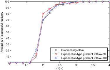
Figure 1. Empirical success rate versus $m/nr$ for $X\in{\mathbb{R}}^{n\times r}$ with $n=200$, $r=2$.

Example 6.2.

In this example, we test the convergence and robustness of the exponential-type gradient descent algorithm. We use noiseless model for (a) to test the convergence and use the noise model for (b) to test the robustness. The noise model is described as $y_{i}=a_{i}^{\top}XX^{\top}a_{i}+\epsilon_{i}$ where the noise $\epsilon_{i}\sim\mathcal{N}(0,0.1^{2}),\;i=1,\ldots,m$. Let $X\in{\mathbb{R}}^{n\times r}$ with $n=200,r=2$, the parameter $\alpha_{y}=9$ in spectral initialization and the step size $\mu=0.1\cdot m/\sum_{i=1}^{m}y_{i}$. We consider the performance with $\alpha=20$ and $100$. We set the number of measurements $m=3nr$. Figure 2 depicts the relative error against the iteration number. From the figure, we observe that our exponential-type gradient descent algorithm can converge to the exact solution and is robust with noisy measurements.

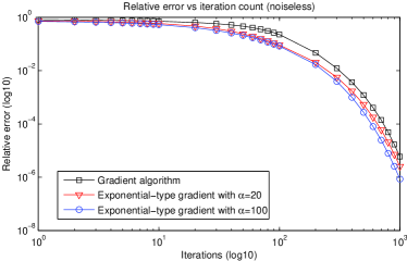
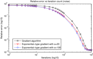
Figure 2. Relative error with respect to noiseless and noise, where the unknown matrix $X\in{\mathbb{R}}^{n\times r}$ with $n=200$, $r=2$ and $m=3nr$.

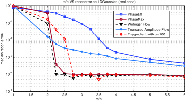
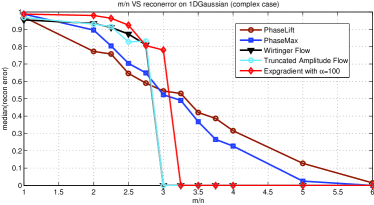
Figure 3. Relative error versus $m/n$ for real and complex signals $x$ with dimension $n=100$.

Example 6.3.

Finally, we test the performance of the exponential-type gradient descent algorithm to recover $X\in{\mathbb{R}}^{n\times r}$ with $r=1$. As stated before, under the setting of $r=1$, the (1) is reduced to phase retrieval problem. One already develops many algorithms to solve phase retrieval problems, such as PhaseLift [5], PhaseMax [15], WirtFlow [3], and TAF [28]. The aim of numerical experiments is to compare the performance of the exponential-type gradient descent algorithm with that of other existing methods for phase retrieval as mentioned above. This experiment is done by Phasepack [6] which is a algorithm package for solving the phase retrieval problem. For the exponential-type gradient algorithm, we choose the parameter $\alpha_{y}=9$ and $\alpha=100$ as the comparison. We choose a random real signal $x\in{\mathbb{R}}^{n}$ in (a) and a random complex signal $x\in\mathbb{C}^{n}$ in (b) with $n=100$. Here, one can use the elegant formulation of Wirtinger derivatives [3] to obtain the exponential-type gradient for complex signal. We show the relative error in the reconstructed signal as a function of the the number of measurements $m$, where $m$ within the ranges $[n,6n]$. The results are shown in Figure 3. From the figure, we can see that our algorithm performs well comparing with state-of-the-art phase retrieval algorithms.

7. Appendix

7.1. Proof of Theorem 4.1

Proof.

By homogeneity, it suffices to consider the case where $\|{X}\|_{F}=1$. We assume that $X=(x_{1},\ldots,x_{r})\in{\mathbb{R}}^{n\times r}$ has orthogonal columns satisfying $\|{x_{1}}\|_{2}\geq\cdots\geq\|{x_{r}}\|_{2}$. Recall that $\sigma_{1}\geq\sigma_{2}\geq\cdots\geq\sigma_{r}>0$ are the nonzero eigenvalues of the positive semidefinite matrix $XX^{\top}$ and then

$$\sigma_{j}=\|{x_{j}}\|_{2}^{2},\quad\text{ for }\;1\leq j\leq r.$$

From Lemma 2.3, for $\varepsilon>0$, we have

(20) $$\frac{1}{m}\sum_{k=1}^{m}a_{k}^{\top}XX^{\top}a_{k}=\frac{1}{m}\sum_{k=1}^{m}y_{k}\in[1-\varepsilon,1+\varepsilon],$$

with probability at least $1-2\exp(-\Omega(n))$, if $m\geq Cn$ where $C$ is a constant depending on $\varepsilon$. Here, we use the fact that $\|XX^{\top}\|_{*}=\|X\|_{F}^{2}=1$. The (20) implies that

(21) $${\mathds{1}}_{\{y_{i}\leq(1-\varepsilon)\alpha_{y}\}}\leq{\mathds{1}}_{\{y_{i}\leq\frac{\alpha_{y}}{m}\sum_{k=1}^{m}y_{k}\}}\leq{\mathds{1}}_{\{y_{i}\leq(1+\varepsilon)\alpha_{y}\}}.$$

Recall that $Y=\frac{1}{m}\sum_{i=1}^{m}y_{i}a_{i}a_{i}^{\top}{\mathds{1}}_{\{y_{i}\leq\frac{\alpha_{y}}{m}\sum_{k=1}^{m}y_{k}\}}$. The (21) implies that

(22) $$Y_{2}\preceq Y\preceq Y_{1}$$

holds with high probability where

$$Y_{2}:=\frac{1}{m}\sum_{i=1}^{m}y_{i}a_{i}a_{i}^{\top}{\mathds{1}}_{\{y_{i}\leq(1-\varepsilon)\alpha_{y}\}},\quad Y_{1}:=\frac{1}{m}\sum_{i=1}^{m}y_{i}a_{i}a_{i}^{\top}{\mathds{1}}_{\{y_{i}\leq(1+\varepsilon)\alpha_{y}\}}.$$

We claim the following results:

Claim 7.1.

For any $0<\delta<1$, if $\alpha_{y}\geq C\sqrt{\log(cr\sigma_{1}/\delta)}$, then

(23) $$\|{{\mathbb{E}}Y_{1}-2XX^{\top}-I}\|_{2}\leq\delta,\qquad\|{{\mathbb{E}}Y_{2}-2XX^{\top}-I}\|_{2}\leq\delta.$$

The (23) implies that $\|{{\mathbb{E}}Y_{1}}\|_{2}\geq 1+2\sigma_{1}-\delta$ and $\|{{\mathbb{E}}Y_{2}}\|_{2}\geq 1+2\sigma_{1}-\delta$. We can use Lemma 2.1 to obtain that if $m\geq C\delta^{-2}(1+2\sigma_{1}-\delta)^{-2}n$, and then with probability at least $1-4\exp(-\Omega(n))$, we have

(24) $$\|{Y_{1}-{\mathbb{E}}Y_{1}}\|_{2}\leq\delta,\qquad\|{Y_{2}-{\mathbb{E}}Y_{2}}\|_{2}\leq\delta,$$

where $C$ is a positive constant. Indeed, in Lemma 2.1 we take the $i$-th row of $A$ as $b_{i}^{\top}:=\sqrt{y_{i}}a_{i}^{\top}{\mathds{1}}_{\{y_{i}\leq(1+\varepsilon)\alpha_{y}\}}$ and set $\Sigma={\mathbb{E}}Y_{1}$ with $\|{{\mathbb{E}}Y_{1}}\|_{2}\geq 1+2\sigma_{1}-\delta$ and $t=\delta\|{{\mathbb{E}}Y_{1}}\|_{2}\sqrt{m}$. Then we can obtain $\|{Y_{1}-{\mathbb{E}}Y_{1}}\|_{2}\leq\delta$. Similarly, we have $\|{Y_{2}-{\mathbb{E}}Y_{2}}\|_{2}\leq\delta$ if we take the $i$-th row of $A$ as $b_{i}^{\top}:=\sqrt{y_{i}}a_{i}^{\top}{\mathds{1}}_{\{y_{i}\leq(1-\varepsilon)\alpha_{y}\}}$ and set $\Sigma:={\mathbb{E}}Y_{2}$.

Combining (22), (23) and (24), we have

(25) $$\|{Y-2XX^{\top}-I}\|_{2}\leq 2\delta$$

with probability at least $1-6\exp(-\Omega(n))$ provided $m\geq C\delta^{-2}(1+2\sigma_{1}-\delta)^{-2}n$ and $\alpha_{y}\geq C\sqrt{\log(cr\sigma_{1}/\delta)}$. Furthermore, from Wely Theorem we have

(26) $$|\lambda_{r+1}-1|\leq 2\delta\quad\text{and}\quad|\lambda_{n}-1|\leq 2\delta.$$

Next, we turn to consider $d(U_{0})$. Recall the definition $U_{0}=U\Sigma^{1/2}$ in Algorithm 1. Here, $U=(u_{1},\ldots,u_{r})$ where $u_{k}$ is normalized eigenvectors corresponding to the eigenvalues $\lambda_{k}$ of $Y$ for $k=1,\ldots,r$, and the scaling of the diagonal matrix $\Sigma$ is given by $\Sigma_{i,i}=(\lambda_{i}-\lambda_{r+1})/2$. Hence,

$$\|{U_{0}U_{0}^{\top}-XX^{\top}}\|_{2} \leq \|{U_{0}U_{0}^{\top}-\frac{1}{2}Y+\frac{1}{2}\lambda_{r+1}I}\|_{2}+\|{\frac{1}{2}Y-\frac{1}{2}I-XX^{\top}}\|_{2}+\frac{1}{2}\|{(\lambda_{r+1}-1)I}\|_{2}$$

$$\leq \frac{1}{2}(\lambda_{r+1}-\lambda_{n})+\delta+\frac{1}{2}(\lambda_{r+1}-1)$$

$$\leq 4\delta,$$

where the second inequality follows from (25) and the last inequality follows from (26). Then, using the following fact ( see, e.g. the Initialization of [30])

$$\mathop{\min}\limits_{O\in\mathcal{O}(r)}\|U_{0}-XO\|_{F}^{2} \leq \frac{\|{U_{0}U_{0}^{\top}-XX^{\top}}\|_{F}^{2}}{(2\sqrt{2}-2)\sigma_{r}},$$

and taking $\delta\leq\frac{\sigma_{r}}{18\sqrt{r}}$, we obtain

$$\mathop{\min}\limits_{O\in\mathcal{O}(r)}\|U_{0}-XO\|_{F}^{2} \leq \frac{2r\|{U_{0}U_{0}^{\top}-XX^{\top}}\|_{2}^{2}}{(2\sqrt{2}-2)\sigma_{r}}$$

$$\leq \frac{32r\delta^{2}}{(2\sqrt{2}-2)\sigma_{r}}$$

$$\leq \frac{\sigma_{r}}{8},$$

where we use $\|{A}\|_{F}\leq\sqrt{{\rm rank}(A)}\|{A}\|_{2}$ in the first inequality. The choice of $\delta$ implies that the measurements $m\geq C\sigma_{r}^{-2}nr$ and $\alpha_{y}\geq C\sqrt{\log(c^{\prime}\kappa r)}$, where $\kappa=\sigma_{1}/\sigma_{r}$ denotes the ratio of the largest to the smallest nonzero eigenvalues of matrix $XX^{\top}$.

We remain to prove Claim 7.1. There exists an orthogonal matrix $O\in{\mathbb{R}}^{r\times r}$ such that $X=O(\|{x_{1}}\|_{2}e_{1},\ldots,\|{x_{r}}\|_{2}e_{r})$. Then

$$O^{\top}({\mathbb{E}}Y_{1}-2XX^{\top}-I)O = O^{\top}{\mathbb{E}}Y_{1}O-\left(2\sum_{k=1}^{r}\|{x_{k}}\|_{2}^{2}e_{k}e_{k}^{\top}+I\right),$$

and

(27) $$O^{\top}{\mathbb{E}}Y_{1}O = {\mathbb{E}}\left[\sum_{k=1}^{r}\|{x_{k}}\|_{2}^{2}a_{i,k}^{2}a_{i}a_{i}^{\top}{\mathds{1}}_{\{\sum_{k=1}^{r}\|{x_{k}}\|_{2}^{2}a_{i,k}^{2}\leq(1+\varepsilon)\alpha_{y}\}}\right].$$

A simple calculation is that

(28) $${\mathbb{E}}\left[\sum_{k=1}^{r}\|{x_{k}}\|_{2}^{2}a_{i,k}^{2}a_{i}a_{i}^{\top}\right]=2\sum_{k=1}^{r}\|{x_{k}}\|_{2}^{2}e_{k}e_{k}^{\top}+I,$$

which implies that

(29) $$O^{\top}{\mathbb{E}}Y_{1}O\leq 2\sum_{k=1}^{r}\|{x_{k}}\|_{2}^{2}e_{k}e_{k}^{\top}+I,$$

where we write $M_{2}\leq M_{1}$ if all entries of $M_{1}-M_{2}$ are nonnegative. On the other hand, from (27) we obtain that

(30) $$O^{\top}{\mathbb{E}}Y_{1}O={\mathbb{E}}\left[\sum_{k=1}^{r}\|{x_{k}}\|_{2}^{2}a_{i,k}^{2}a_{i}a_{i}^{\top}\right]-{\mathbb{E}}\left[\sum_{k=1}^{r}\|{x_{k}}\|_{2}^{2}a_{i,k}^{2}a_{i}a_{i}^{\top}{\mathds{1}}_{\{\sum_{k=1}^{r}\|{x_{k}}\|_{2}^{2}a_{i,k}^{2}\geq(1+\varepsilon)\alpha_{y}\}}\right].$$

For any $1\leq j,l,k\leq r$ and $\delta>0$, by Hölder’s inequality we have

(31) $${\mathbb{E}}\left[\|{x_{k}}\|_{2}^{2}a_{i,j}^{2}a_{i,l}^{2}{\mathds{1}}_{\{\sum_{k=1}^{r}\|{x_{k}}\|_{2}^{2}a_{i,k}^{2}\geq(1+\varepsilon)\alpha_{y}\}}\right]$$

$$\quad\leq\|{x_{1}}\|_{2}^{2}\sqrt{{\mathbb{E}}[a_{i,j}^{4}a_{i,l}^{4}]}\cdot\sqrt{{\mathbb{P}}\left\{\sum_{k=1}^{r}\|{x_{k}}\|_{2}^{2}a_{i,k}^{2}\geq(1+\varepsilon)\alpha_{y}\right\}}$$

$$\quad\leq C_{1}\|{x_{1}}\|_{2}^{2}\exp\left(-C_{0}\min\Big{(}\frac{(1+\varepsilon)^{2}\alpha_{y}^{2}}{\|{x_{1}}\|_{2}^{4}+\cdots+\|{x_{r}}\|_{2}^{4}},\frac{(1+\varepsilon)\alpha_{y}}{\|{x_{1}}\|_{2}^{2}}\Big{)}\right)$$

$$\quad\leq C_{1}\sigma_{1}\exp\left(-C_{0}(1+\varepsilon)^{2}\alpha_{y}^{2}\right)$$

$$\quad\leq\frac{\delta}{r}$$

provided $\alpha_{y}\geq C\sqrt{\log(cr\sigma_{1}/\delta)}$, where the second inequality follows from Lemma 2.2 and the third inequality follows from the fact that $\|{X}\|_{F}=1$ and $\|{x_{r}}\|_{2}\leq\cdots\leq\|{x_{1}}\|_{2}\leq 1$. The (31) implies that

(32) $${\mathbb{E}}\left[\sum_{k=1}^{r}\|{x_{k}}\|_{2}^{2}a_{i,k}^{2}a_{i}a_{i}^{\top}{\mathds{1}}_{\{\sum_{k=1}^{r}\|{x_{k}}\|_{2}^{2}a_{i,k}^{2}\geq(1+\varepsilon)\alpha_{y}\}}\right]\leq\delta I.$$

Thus, combining (28), (30) and (32) we have

(33) $$O^{\top}{\mathbb{E}}Y_{1}O \geq 2\sum\limits_{k=1}^{r}\|{x_{k}}\|_{2}^{2}e_{k}e_{k}^{\top}+(1-\delta)I.$$

Combining (29) and (33) and noting that $O^{\top}{\mathbb{E}}Y_{1}O$ is a diagonal matrix, we obtain

$$\|{{\mathbb{E}}Y_{1}-2XX^{\top}-I}\|_{2} = \|{O^{\top}({\mathbb{E}}Y_{1}-2XX^{\top}-I)O}\|_{2}\leq\delta.$$

Similarly, we can obtain $\|{{\mathbb{E}}Y_{2}-2XX^{\top}-I}\|_{2}\leq\delta$, which completes the proof. ∎

7.2. Proof of Proposition 5.4

We always assume that $\|{X}\|_{F}=1$ throughout the proof. We set $H:=U-{\bar{X}}$ where ${\bar{X}}=\mathop{\rm argmin}\limits_{Z\in\mathcal{X}}\|{U-Z}\|_{F}$ and $\mathcal{X}$ is the solution set. Then the exponential-type gradient can be rewritten as

(34) $$\nabla f_{{\rm ex}}(U)=\frac{1}{m}\sum_{i=1}^{m}(a_{i}^{\top}HH^{\top}a_{i}+2a_{i}^{\top}H{\bar{X}}^{\top}a_{i})(a_{i}a_{i}^{\top}H+a_{i}a_{i}^{\top}{\bar{X}})\cdot\exp\left(-\frac{my_{i}}{\alpha\sum_{k=1}^{m}y_{k}}\right).$$

For convenience, we let

(35) $$\rho_{i,\alpha}\,\,:=\,\,\exp\big{(}-\frac{my_{i}}{\alpha\sum_{i=1}^{m}y_{i}}\big{)},\;i=1,\ldots,m.$$

To prove Proposition 5.4, we need the following lemmas.

Lemma 7.2.

For any fixed $\alpha\geq 20$ and $\delta>0$, if $m\geq c_{0}\alpha^{2}\delta^{-2}nr\log(\sqrt{r}/\delta)$, then with probability at least $1-C\exp(-\Omega(\alpha^{-2}\delta^{2}m))$, the followings hold for all non-zero matrix $U\in{\mathbb{R}}^{n\times r}$:

$$(a) \frac{1}{m}\sum_{i=1}^{m}(a_{i}^{\top}H{\bar{X}}^{\top}a_{i})^{2}\rho_{i,\alpha}\geq (0.78\sigma_{r}-2\delta)\|{H}\|_{F}^{2}+0.78{\rm tr}^{2}(H^{\top}{\bar{X}})+0.78\|{H^{\top}{\bar{X}}}\|_{F}^{2}$$

$$(b) \frac{1}{m}\sum_{i=1}^{m}(a_{i}^{\top}H{\bar{X}}^{\top}a_{i})^{2}\rho_{i,\alpha}\leq (\sigma_{1}+2\delta)\|{H}\|_{F}^{2}+{\rm tr}^{2}(H^{\top}{\bar{X}})+\|{H^{\top}{\bar{X}}}\|_{F}^{2},$$

where $C,c_{0}$ are universal constants.

Proof.

Suppose for the moment that $H$ is independent from $a_{i}$. By homogeneity, it suffices to establish the claim for the case $\|{H}\|_{F}=1$. From (20) we have

(36) $$\exp\Big{(}-\frac{a_{i}^{\top}XX^{\top}a_{i}}{0.99\alpha}\Big{)}\leq\rho_{i,\alpha}\leq\exp\Big{(}-\frac{a_{i}^{\top}XX^{\top}a_{i}}{1.01\alpha}\Big{)}$$

with high probability. For convenience, we set

(37) $$\bar{\rho}_{i,\alpha}:=\exp\Big{(}-\frac{a_{i}^{\top}{\bar{X}}{\bar{X}}^{\top}a_{i}}{0.99\alpha}\Big{)},\;i=1,\ldots,m.$$

Noting that $a_{i}^{\top}{\bar{X}}{\bar{X}}^{\top}a_{i}=a_{i}^{\top}XX^{\top}a_{i}$, we have

(38) $$\frac{1}{m}\sum_{i=1}^{m}(a_{i}^{\top}H{\bar{X}}^{\top}a_{i})^{2}\rho_{i,\alpha}\geq\frac{1}{m}\sum_{i=1}^{m}(a_{i}^{\top}H{\bar{X}}^{\top}a_{i})^{2}\bar{\rho}_{i,\alpha}.$$

We claim the following results:

Claim 7.3.

For any fixed parameter $\alpha\geq 20$ it holds

• ${\mathbb{E}}\left[(a_{i}^{\top}H{\bar{X}}^{\top}a_{i})^{2}\right]\geq\sigma_{r}\|{H}\|_{F}^{2}+{\rm tr}^{2}(H^{\top}{\bar{X}})+\|{H^{\top}{\bar{X}}}\|_{F}^{2}$

• ${\mathbb{E}}\left[(a_{i}^{\top}H{\bar{X}}^{\top}a_{i})^{2}\right]\leq\sigma_{1}\|{H}\|_{F}^{2}+{\rm tr}^{2}(H^{\top}{\bar{X}})+\|{H^{\top}{\bar{X}}}\|_{F}^{2}$

• ${\mathbb{E}}\left[(a_{i}^{\top}H{\bar{X}}^{\top}a_{i})^{2}\bar{\rho}_{i,\alpha}\right]\geq 0.78{\mathbb{E}}\left[(a_{i}^{\top}H{\bar{X}}^{\top}a_{i})^{2}\right]$.

Then combining 3) and 1) we obtain that

$${\mathbb{E}}\left[(a_{i}^{\top}H{\bar{X}}^{\top}a_{i})^{2}\bar{\rho}_{i,\alpha}\right] \geq 0.78\sigma_{r}\|{H}\|_{F}^{2}+0.78{\rm tr}^{2}(H^{\top}{\bar{X}})+0.78\|{H^{\top}{\bar{X}}}\|_{F}^{2}.$$

Since

$$(a_{i}^{\top}H{\bar{X}}^{\top}a_{i})^{2}\bar{\rho}_{i,\alpha} \leq (a_{i}^{\top}{\bar{X}}{\bar{X}}^{\top}a_{i})\bar{\rho}_{i,\alpha}(a_{i}^{\top}HH^{\top}a_{i})$$

and $(a_{i}^{\top}{\bar{X}}{\bar{X}}^{\top}a_{i})\bar{\rho}_{i,\alpha}$ is bounded, it means that $(a_{i}^{\top}H{\bar{X}}^{\top}a_{i})^{2}\bar{\rho}_{i,\alpha}$ is a sub-exponential random variable with $\psi_{1}$ norm $O(\alpha\|{H}\|_{F}^{2})$. We can use Lemma 2.2 to obtain that

(39) $$\frac{1}{m}\sum_{i=1}^{m}(a_{i}^{\top}H{\bar{X}}^{\top}a_{i})^{2}\bar{\rho}_{i,\alpha} \geq{\mathbb{E}}\big{[}(a_{i}^{\top}H{\bar{X}}^{\top}a_{i})^{2}\bar{\rho}_{i,\alpha}\big{]}-\delta\|{H}\|_{F}^{2}$$

$$\geq(0.78\sigma_{r}-\delta)\|{H}\|_{F}^{2}+0.78{\rm tr}^{2}(H^{\top}{\bar{X}})+0.78\|{H^{\top}{\bar{X}}}\|_{F}^{2}$$

holds with probability at least $1-\exp(-\Omega(\alpha^{-2}\delta^{2}m))$ where $\delta>0$. Combining (38) and (39), we obtain that (a) holds for a fixed $H\in{\mathbb{R}}^{n\times r}$.

We construct an $\epsilon$-net $\mathcal{N}_{\epsilon}\subset{\mathbb{R}}^{n\times r}$ with cardinality $|\mathcal{N}_{\epsilon}|\leq(1+\frac{2}{\epsilon})^{nr}$ such that for any $H\in{\mathbb{R}}^{n\times r}$ with $\|{H}\|_{F}=1$, there exists $H_{0}\in\mathcal{N}_{\epsilon}$ satisfying $\|{H-H_{0}}\|_{F}\leq\epsilon$. Taking a union bound over this set gives that

$$\frac{1}{m}\sum_{i=1}^{m}(a_{i}^{\top}H_{0}{\bar{X}}^{\top}a_{i})^{2}\bar{\rho}_{i,\alpha} \geq (0.78\sigma_{r}-\delta)\|{H_{0}}\|_{F}^{2}+0.78{\rm tr}^{2}(H_{0}^{\top}{\bar{X}})+0.78\|{H_{0}^{\top}{\bar{X}}}\|_{F}^{2}$$

holds for all $H_{0}\in\mathcal{N}_{\epsilon}$ with probability at least $1-(1+\frac{2}{\epsilon})^{nr}\exp(-\Omega(\alpha^{-2}\delta^{2}m))$.
Note that $\bar{\rho}_{i,\alpha}<1$ for all $i$. Then there exists a universal constant $c_{1}>0$ such that

(40) $$\left|\frac{1}{m}\sum_{i=1}^{m}(a_{i}^{\top}H{\bar{X}}^{\top}a_{i})^{2}\bar{\rho}_{i,\alpha}-\frac{1}{m}\sum_{i=1}^{m}(a_{i}^{\top}H_{0}{\bar{X}}^{\top}a_{i})^{2}\bar{\rho}_{i,\alpha}\right| \leq \frac{1}{m}\sum_{i=1}^{m}\left|a_{i}^{\top}H{\bar{X}}^{\top}a_{i}-a_{i}^{\top}H_{0}{\bar{X}}^{\top}a_{i}\right|$$

$$\leq c_{1}\|HX^{\top}-H_{0}X^{\top}\|_{*}$$

$$\leq c_{1}\sqrt{r}\|{H-H_{0}}\|_{F}$$

$$\leq c_{1}\sqrt{r}\epsilon$$

where we use Lemma 2.3 in the second line, the fact $\|A\|_{*}\leq\sqrt{{\rm rank}(A)}\|{A}\|_{F}$ in the third line. Indeed, according to Lemma 2.3, for any $\delta\in(0,1)$, if $m\geq c_{0}\delta^{-2}n$, then with probability at least $1-C\exp(-\Omega(n))$ we have

$$\frac{1}{m}\sum\limits_{i=1}^{m}\left|a_{i}^{\top}HX^{\top}a_{i}-a_{i}^{\top}H_{0}X^{\top}a_{i}\right|\leq(1+\delta)\|HX^{\top}-H_{0}X^{\top}\|_{*}\leq c_{1}\|HX^{\top}-H_{0}X^{\top}\|_{*}.$$

By choosing $\epsilon=\frac{\delta}{c_{1}\sqrt{r}}$ in (40), we conclude the first part of lemma.

We now turn to the part (b). The (36) implies that

$$\rho_{i,\alpha}\leq\exp\big{(}-\frac{a_{i}^{\top}XX^{\top}a_{i}}{1.01\alpha}\big{)}$$

holds with high probability. It gives that

$$\frac{1}{m}\sum_{i=1}^{m}(a_{i}^{\top}H{\bar{X}}^{\top}a_{i})^{2}\rho_{i,\alpha} \leq \frac{1}{m}\sum_{i=1}^{m}(a_{i}^{\top}H{\bar{X}}^{\top}a_{i})^{2}\exp\left(-\frac{a_{i}^{\top}XX^{\top}a_{i}}{1.01\alpha}\right).$$

From Claim 7.3, we have

$${\mathbb{E}}\left[(a_{i}^{\top}H{\bar{X}}^{\top}a_{i})^{2}\exp\left(-\frac{a_{i}^{\top}XX^{\top}a_{i}}{1.01\alpha}\right)\right] \leq \sigma_{1}\|{H}\|_{F}^{2}+{\rm tr}^{2}(H^{\top}{\bar{X}})+\|{H^{\top}{\bar{X}}}\|_{F}^{2}.$$

Similarly, $(a_{i}^{\top}H{\bar{X}}^{\top}a_{i})^{2}\exp\big{(}-\frac{a_{i}^{\top}XX^{\top}a_{i}}{1.01\alpha}\big{)}$ is a sub-exponential random variable with sub-exponential norm $O(\alpha\|{H}\|_{F}^{2})$. Then, we can employ the method for proving part (a) to prove part (b). ∎

Lemma 7.4.

For a fixed $\lambda>0$, for any $H\in{\mathbb{R}}^{n\times r}$ and $\delta>0$, if $m\geq c_{0}\delta^{-2}\lambda^{-2}nr\log(\sqrt{r}/(\delta\lambda))$, then with probability at least $1-C\exp(-\Omega(\delta^{2}\lambda^{2}m))$, we have

$$\frac{1}{m}\sum_{i=1}^{m}(a_{i}^{\top}HH^{\top}a_{i})^{2}\exp\left(-\lambda\frac{a_{i}^{\top}HH^{\top}a_{i}}{\|{H}\|_{F}^{2}}\right)\leq 2\|{HH^{\top}}\|_{F}^{2}+(2\delta+1)\|{H}\|_{F}^{4}.$$

Here, $c_{0},C$ are some universal constants.

Proof.

Without loss of generality, we only need to prove the lemma in the case $\|{H}\|_{F}=1$. It is straightforward to show that

$${\mathbb{E}}\left[(a_{i}^{\top}HH^{\top}a_{i})^{2}\exp\left(-\lambda a_{i}^{\top}HH^{\top}a_{i}\right)\right]\leq{\mathbb{E}}\left[(a_{i}^{\top}HH^{\top}a_{i})^{2}\right]=2\|{HH^{\top}}\|_{F}^{2}+\|{H}\|_{F}^{4}.$$

Observe that $(a_{i}^{\top}HH^{\top}a_{i})^{2}\exp\big{(}-\lambda a_{i}^{\top}HH^{\top}a_{i}\big{)}$ is a sub-exponential random variable with sub-exponential norm $O(1/\lambda\cdot\|{H}\|_{F}^{2})$. According to Lemma 2.2 we have

$$\frac{1}{m}\sum_{i=1}^{m}(a_{i}^{\top}HH^{\top}a_{i})^{2}\exp\left(-\lambda a_{i}^{\top}HH^{\top}a_{i}\right)\leq 2\|{HH^{\top}}\|_{F}^{2}+\|{H}\|_{F}^{4}+\frac{\delta_{0}}{\lambda}\|{H}\|_{F}^{2}$$

with probability $1-\exp(-\Omega(\delta_{0}^{2}m))$. We next construct an $\epsilon$-net $\mathcal{N}_{\epsilon}$ with $|\mathcal{N}_{\epsilon}|\leq(1+\frac{2}{\epsilon})^{nr}$ such that for any $H\in{\mathbb{R}}^{n\times r}$ with $\|{H}\|_{F}=1$, there exists $H_{0}\in\mathcal{N}_{\epsilon}$ satisfying $\|{H-H_{0}}\|_{F}\leq\epsilon$. Since $x^{2}e^{-\lambda x}$ is Lipschitz function with Lipschitz constant $O(1/\lambda^{2})$, we have

$$\begin{array}[]{l}\Big{|}\frac{1}{m}\sum_{i=1}^{m}(a_{i}^{\top}HH^{\top}a_{i})^{2}\exp\Big{(}-\lambda a_{i}^{\top}HH^{\top}a_{i}\Big{)}-\frac{1}{m}\sum_{i=1}^{m}(a_{i}^{\top}H_{0}H_{0}^{\top}a_{i})^{2}\exp\Big{(}-\lambda a_{i}^{\top}H_{0}H_{0}^{\top}a_{i}\Big{)}\Big{|}\vspace{1ex}\\ \leq\frac{1}{\lambda^{2}m}\sum_{i=1}^{m}\Big{|}a_{i}^{\top}HH^{\top}a_{i}-a_{i}^{\top}H_{0}H_{0}^{\top}a_{i}\Big{|}\vspace{1ex}\\ \leq\frac{c_{2}\sqrt{r}\epsilon}{\lambda^{2}}\end{array}$$

where the last inequality follows from Lemma 2.3. By choosing $\epsilon=\frac{\delta_{0}\lambda}{c_{2}\sqrt{r}}$, we obtain

$$\frac{1}{m}\sum_{i=1}^{m}(a_{i}^{\top}HH^{\top}a_{i})^{2}\exp\left(-\lambda a_{i}^{\top}HH^{\top}a_{i}\right)\leq 2\|{HH^{\top}}\|_{F}^{2}+\|{H}\|_{F}^{4}+\frac{2\delta_{0}}{\lambda}\|{H}\|_{F}^{2}$$

with probability at least $1-\exp(-\Omega(\delta_{0}^{2}m))$ if $m\geq c_{0}\delta_{0}^{-2}nr\log(\sqrt{r}/(\delta_{0}\lambda))$. Finally, noting that $\|{H}\|_{F}=1$ and taking $\delta_{0}=\lambda\delta$, we arrive at the conclusion. ∎

Corollary 7.5.

For any $\delta>0$, $U\in{\mathbb{R}}^{n\times r}$ and $H=U-{\bar{X}}$, if $m\geq c_{0}\alpha^{2}\delta^{-2}\sigma_{r}^{-2}nr\log(\alpha\sqrt{r}/(\delta\sigma_{r}))$, then with probability at least $1-C\exp(-\Omega(n))$, it holds

$$\frac{1}{m}\sum_{i=1}^{m}(a_{i}^{\top}HH^{\top}a_{i})^{2}\rho_{i,\alpha}\leq 2\|{HH^{\top}}\|_{F}^{2}+(2\delta+1)\|{H}\|_{F}^{4}.$$

Proof.

Since $\sigma_{r}$ is the smallest eigenvalue of $XX^{\top}$, we have

$$y_{i}=a_{i}^{\top}XX^{\top}a_{i}\geq\sigma_{r}\|{a_{i}}\|^{2},$$

which implies that

(41) $$\|{a_{i}}\|^{2}\leq\frac{a_{i}^{\top}XX^{\top}a_{i}}{\sigma_{r}}=\frac{y_{i}}{\sigma_{r}}.$$

On the other hand, we have

(42) $$a_{i}^{\top}HH^{\top}a_{i}\leq\|H\|_{F}^{2}\|a_{i}\|^{2}.$$

Combining (41) and (42), we obtain that

(43) $$y_{i}\geq\sigma_{r}\frac{a_{i}^{\top}HH^{\top}a_{i}}{\|H\|_{F}^{2}}.$$

According to (36) and (43), we obtain that

$$\frac{1}{m}\sum_{i=1}^{m}(a_{i}^{\top}HH^{\top}a_{i})^{2}\rho_{i,\alpha} \leq \frac{1}{m}\sum_{i=1}^{m}(a_{i}^{\top}HH^{\top}a_{i})^{2}\exp\left(-\frac{\sigma_{r}}{1.01\alpha}\cdot\frac{a_{i}^{\top}HH^{\top}a_{i}}{\|{H}\|_{F}^{2}}\right).$$

We take $\lambda=\frac{\sigma_{r}}{1.01\alpha}$ in Lemma 7.4 and arrive at the conclusion. ∎

Proof of Proposition 5.4 .

To state conveniently, we set

$$\beta^{2}=\frac{1}{m}\sum_{i=1}^{m}(a_{i}^{\top}HH^{\top}a_{i})^{2}\rho_{i,\alpha},\quad\gamma^{2}=\frac{2}{m}\sum_{i=1}^{m}(a_{i}^{\top}H{\bar{X}}^{\top}a_{i})^{2}\rho_{i,\alpha}.$$

According to the expression of exponential-type gradient (34), we have

$$\langle\nabla f_{{\rm ex}}(U),H\rangle =\beta^{2}+\gamma^{2}+\frac{3}{m}\sum\limits_{i=1}^{m}(a_{i}^{\top}H{\bar{X}}^{\top}a_{i})(a_{i}^{\top}HH^{\top}a_{i})\rho_{i,\alpha}$$

$$\geq\beta^{2}+\gamma^{2}-\frac{3}{m}\sqrt{\sum\limits_{i=1}^{m}(a_{i}^{\top}H{\bar{X}}^{\top}a_{i})^{2}\rho_{i,\alpha}}\cdot\sqrt{\sum\limits_{i=1}^{m}(a_{i}^{\top}HH^{\top}a_{i})^{2}\rho_{i,\alpha}}$$

$$=\beta^{2}+\gamma^{2}-\frac{3}{\sqrt{2}}\beta\gamma=\Big{(}\gamma-\frac{3}{2\sqrt{2}}\beta\Big{)}^{2}-\frac{1}{8}\beta^{2}$$

$$\geq\Big{(}\frac{\gamma^{2}}{2}-\frac{9}{8}\beta^{2}\Big{)}-\frac{1}{8}\beta^{2}=\frac{\gamma^{2}}{2}-\frac{5}{4}\beta^{2}$$

$$=\frac{1}{m}\sum_{i=1}^{m}(a_{i}^{\top}H{\bar{X}}^{\top}a_{i})^{2}\rho_{i,\alpha}-\frac{5}{4m}\sum_{i=1}^{m}(a_{i}^{\top}HH^{\top}a_{i})^{2}\rho_{i,\alpha}$$

$$\geq(0.78\sigma_{r}-2\delta_{1})\|{H}\|_{F}^{2}+0.78{\rm tr}^{2}(H^{\top}{\bar{X}})+0.78\|{H^{\top}{\bar{X}}}\|_{F}^{2}-\frac{5}{2}\|{HH^{\top}}\|_{F}^{2}-\frac{5(2\delta_{2}+1)}{4}\|{H}\|_{F}^{4}$$

$$\geq\left(0.78\sigma_{r}-2\delta_{1}-\frac{5(2\delta_{2}+3)}{4}\|{H}\|_{F}^{2}\right)\|{H}\|_{F}^{2}+0.78\left({\rm tr}^{2}(H^{\top}{\bar{X}})+\|{H^{\top}{\bar{X}}}\|_{F}^{2}\right)$$

where we use Cauchy-Schwarz inequality in the second line, the inequality $(\gamma-\beta)^{2}\geq\frac{\gamma^{2}}{2}-\beta^{2}$ in the fourth line, Lemma 7.2 and Corollary 7.5 in the sixth line, and the fact that $\|{HH^{\top}}\|_{F}\leq\|{H}\|_{F}^{2}$ in the last line. Note that $\|{H}\|_{F}^{2}=\|U-{\bar{X}}\|_{F}^{2}=d(U)^{2}\leq\frac{1}{8}\sigma_{r}$. Taking $\delta_{1}\leq\frac{1}{16}\sigma_{r}$ and $\delta_{2}\leq\frac{1}{16}$, we obtain that

$$\langle\nabla f_{{\rm ex}}(U),H\rangle\geq 0.166\sigma_{r}\|{H}\|_{F}^{2}+0.78\left({\rm tr}^{2}(H^{\top}{\bar{X}})+\|{H^{\top}{\bar{X}}}\|_{F}^{2}\right)$$

with probability at least $1-C\exp(-\Omega(n)$, if $m\geq c_{0}\sigma_{r}^{-2}nr\log(c_{1}r/\sigma_{r})$. This implies the part $(a)$.

Next, we turn to the part $(b)$. We consider

$$\|{\nabla f_{{\rm ex}}(U)}\|_{F}^{2}=\mathop{\rm max}\limits_{\|{W}\|_{F}=1,W\in{\mathbb{R}}^{n\times r}}\lvert\langle\nabla f_{{\rm ex}}(U),W\rangle\rvert^{2}$$

on the case where $H=U-{\bar{X}}\leq\sqrt{\frac{1}{8}\sigma_{r}}$. Recall the notation $\rho_{i,\alpha}$ in formula (35), and we have

$$\lvert\langle\nabla f_{{\rm ex}}(U),W\rangle\rvert^{2}$$

$$=\left(\frac{1}{m}\sum_{i=1}^{m}(a_{i}^{\top}HH^{\top}a_{i})(a_{i}^{\top}HW^{\top}a_{i})\rho_{i,\alpha}+\frac{2}{m}\sum_{i=1}^{m}(a_{i}^{\top}H{\bar{X}}^{\top}a_{i})(a_{i}^{\top}HW^{\top}a_{i})\rho_{i,\alpha}\right.$$

$$\quad\left.+\frac{1}{m}\sum_{i=1}^{m}(a_{i}^{\top}HH^{\top}a_{i})(a_{i}^{\top}{\bar{X}}W^{\top}a_{i})\rho_{i,\alpha}+\frac{2}{m}\sum_{i=1}^{m}(a_{i}^{\top}H{\bar{X}}^{\top}a_{i})(a_{i}^{\top}{\bar{X}}W^{\top}a_{i})\rho_{i,\alpha}\right)^{2}$$

$$\leq 4\left(\frac{1}{m}\sum_{i=1}^{m}(a_{i}^{\top}HH^{\top}a_{i})(a_{i}^{\top}HW^{\top}a_{i})\rho_{i,\alpha}\right)^{2}+16\left(\frac{1}{m}\sum_{i=1}^{m}(a_{i}^{\top}H{\bar{X}}^{\top}a_{i})(a_{i}^{\top}HW^{\top}a_{i})\rho_{i,\alpha}\right)^{2}$$

$$\quad+4\left(\frac{1}{m}\sum_{i=1}^{m}(a_{i}^{\top}HH^{\top}a_{i})(a_{i}^{\top}{\bar{X}}W^{\top}a_{i})\rho_{i,\alpha}\right)^{2}+16\left(\frac{1}{m}\sum_{i=1}^{m}(a_{i}^{\top}H{\bar{X}}^{\top}a_{i})(a_{i}^{\top}{\bar{X}}W^{\top}a_{i})\rho_{i,\alpha}\right)^{2}.$$

We first consider the term $4\left(\frac{1}{m}\sum_{i=1}^{m}(a_{i}^{\top}HH^{\top}a_{i})(a_{i}^{\top}HW^{\top}a_{i})\rho_{i,\alpha}\right)^{2}$. Using Cauchy-Schwarz inequality, we obtain that

$$4\left(\frac{1}{m}\sum\limits_{i=1}^{m}(a_{i}^{\top}HH^{\top}a_{i})(a_{i}^{\top}HW^{\top}a_{i})\rho_{i,\alpha}\right)^{2}$$

$$\leq 4\left(\frac{1}{m}\sum\limits_{i=1}^{m}(a_{i}^{\top}HH^{\top}a_{i})^{2}\rho_{i,\alpha}\right)\left(\frac{1}{m}\sum\limits_{i=1}^{m}(a_{i}^{\top}HW^{\top}a_{i})^{2}\rho_{i,\alpha}\right)$$

$$\leq 4\left(\frac{1}{m}\sum\limits_{i=1}^{m}(a_{i}^{\top}HH^{\top}a_{i})^{2}\rho_{i,\alpha}\right)\left(\frac{1}{m}\sum\limits_{i=1}^{m}(a_{i}^{\top}HH^{\top}a_{i})(a_{i}^{\top}WW^{\top}a_{i})\rho_{i,\alpha}\right).$$

According to Corollary 7.5, we have

(44) $$\frac{1}{m}\sum\limits_{i=1}^{m}(a_{i}^{\top}HH^{\top}a_{i})^{2}\rho_{i,\alpha}\leq\left(2\|{HH^{\top}}\|_{F}^{2}+(2\delta_{2}+1)\|{H}\|_{F}^{4}\right)$$

with probability at least $1-C\exp(-\Omega(n))$ provided $m\geq c_{0}\delta_{2}^{-2}\sigma_{r}^{-2}nr\log(\sqrt{r}/(\delta_{2}\sigma_{r}))$. Noting that $a_{i}^{\top}XX^{\top}a_{i}\geq\sigma_{r}\|{a_{i}}\|^{2}$ and $a_{i}^{\top}HH^{\top}a_{i}\leq\|H\|_{F}^{2}\|a_{i}\|^{2}$ we have

$$\frac{a_{i}^{\top}XX^{\top}a_{i}}{2.02\alpha}\geq\frac{\sigma_{r}\cdot a_{i}^{\top}HH^{\top}a_{i}}{2.02\alpha\|{H}\|_{F}^{2}}\qquad\text{and}\qquad\frac{a_{i}^{\top}XX^{\top}a_{i}}{2.02\alpha}\geq\frac{\sigma_{r}\cdot a_{i}^{\top}WW^{\top}a_{i}}{2.02\alpha}.$$

It gives that

(45) $$(a_{i}^{\top}HH^{\top}a_{i})(a_{i}^{\top}WW^{\top}a_{i})\rho_{i,\alpha}$$

$$\leq(a_{i}^{\top}HH^{\top}a_{i})(a_{i}^{\top}WW^{\top}a_{i})\exp\left(-\frac{a_{i}^{\top}XX^{\top}a_{i}}{1.01\alpha}\right)$$

$$\leq(a_{i}^{\top}HH^{\top}a_{i})\exp\left(-\frac{\sigma_{r}\cdot a_{i}^{\top}HH^{\top}a_{i}}{2.02\alpha\|{H}\|_{F}^{2}}\right)(a_{i}^{\top}WW^{\top}a_{i})\exp\left(-\frac{\sigma_{r}\cdot a_{i}^{\top}WW^{\top}a_{i}}{2.02\alpha}\right)$$

$$\leq\|{H}\|_{F}^{2}\Big{(}\frac{1.01\alpha}{e\sigma_{r}}\Big{)}^{2}$$

where we use inequality $xe^{-\gamma x}\leq 1/(e\gamma)$ for any $x\geq 0$ in the last line. Combining formulas (44) and (45), we obtain

$$4\left(\frac{1}{m}\sum\limits_{i=1}^{m}(a_{i}^{\top}HH^{\top}a_{i})(a_{i}^{\top}HW^{\top}a_{i})\rho_{i,\alpha}\right)^{2}\leq 4\Big{(}\frac{1.01\alpha}{e\sigma_{r}}\Big{)}^{2}\|{H}\|_{F}^{2}\left(2\|{HH^{\top}}\|_{F}^{2}+(2\delta_{2}+1)\|{H}\|_{F}^{4}\right).$$

The other three terms can be bounded similarly. For the second term, we have

$$16\left(\frac{1}{m}\sum_{i=1}^{m}(a_{i}^{\top}H{\bar{X}}^{\top}a_{i})(a_{i}^{\top}HW^{\top}a_{i})\rho_{i,\alpha}\right)^{2}$$

$$\leq 16\left(\frac{1}{m}\sum\limits_{i=1}^{m}(a_{i}^{\top}H{\bar{X}}^{\top}a_{i})^{2}\rho_{i,\alpha}\right)\left(\frac{1}{m}\sum\limits_{i=1}^{m}(a_{i}^{\top}HW^{\top}a_{i})^{2}\rho_{i,\alpha}\right)$$

$$\leq 4\Big{(}\frac{1.01\alpha}{e\sigma_{r}}\Big{)}^{2}\|{H}\|_{F}^{2}\left(4(\sigma_{1}+2\delta_{1})\|{H}\|_{F}^{2}+4{\rm tr}^{2}(H^{\top}{\bar{X}})+4\|{H^{\top}{\bar{X}}}\|_{F}^{2}\right)$$

with probability at least $1-C\exp(-\Omega(n))$ provided $m\geq c_{0}\delta_{1}^{-2}nr\log(\sqrt{r}/\delta_{1})$, where we use the part (b) of Lemma 7.2 in the last line. The third term and fourth term can be bounded as

$$4\left(\frac{1}{m}\sum_{i=1}^{m}(a_{i}^{\top}HH^{\top}a_{i})(a_{i}^{\top}{\bar{X}}W^{\top}a_{i})\rho_{i,\alpha}\right)^{2}\leq 4\Big{(}\frac{1.01\alpha}{e\sigma_{r}}\Big{)}^{2}\|{X}\|_{F}^{2}\left(2\|{HH^{\top}}\|_{F}^{2}+(2\delta_{2}+1)\|{H}\|_{F}^{4}\right)$$

$$16\left(\frac{1}{m}\sum_{i=1}^{m}(a_{i}^{\top}H{\bar{X}}^{\top}a_{i})(a_{i}^{\top}{\bar{X}}W^{\top}a_{i})\rho_{i,\alpha}\right)^{2}\leq 4\Big{(}\frac{1.01\alpha}{e\sigma_{r}}\Big{)}^{2}\|{X}\|_{F}^{2}\left(4(\sigma_{1}+2\delta_{1})\|{H}\|_{F}^{2}+4{\rm tr}^{2}(H^{\top}{\bar{X}})+4\|{H^{\top}{\bar{X}}}\|_{F}^{2}\right).$$

Putting there inequalities together and noting that $\|{HH^{\top}}\|_{F}\leq\|{H}\|_{F}^{2}$, we have

$$\|{\nabla f_{{\rm ex}}(U)}\|_{F}^{2}\leq 4\Big{(}\frac{1.01\alpha}{e\sigma_{r}}\Big{)}^{2}\left(\|{H}\|_{F}^{2}+\|{X}\|_{F}^{2}\right)\left(\left(4\sigma_{1}+8\delta_{1}+(2\delta_{2}+3)\|{H}\|_{F}^{2}\right)\|{H}\|_{F}^{2}+4{\rm tr}^{2}(H^{\top}{\bar{X}})+4\|{H^{\top}{\bar{X}}}\|_{F}^{2}\right).$$

Furthermore, noticing that $\|{H}\|_{F}^{2}\leq\frac{1}{8}\sigma_{r}$ and choosing $\delta_{1}\leq\frac{1}{16}\sigma_{r}$, $\delta_{2}\leq\frac{1}{16}$, it follows that

$$\frac{\sigma_{r}^{2}\|{\nabla f_{{\rm ex}}(U)}\|_{F}^{2}}{3\alpha^{2}\left(\|{H}\|_{F}^{2}+\|{X}\|_{F}^{2}\right)}\leq 1.223\sigma_{1}\|{H}\|_{F}^{2}+{\rm tr}^{2}(H^{\top}{\bar{X}})+\|{H^{\top}{\bar{X}}}\|_{F}^{2}$$

with probability at least $1-C\exp(-\Omega(n)$, if $m\geq c_{0}\sigma_{r}^{-2}nr\log(c_{1}r/\sigma_{r})$. ∎

The rest paper is to check the Claim 7.3. For 1) and 2) of the Claim 7.3, let $O_{1}=\mathop{\rm argmin}\limits_{O\in\mathcal{O}(r)}\|{U-XO}\|_{F}$, then ${\bar{X}}=XO_{1}$. Recall that $X$ has orthogonal column vectors, and then there exists an orthogonal matrix $O_{2}\in{\mathbb{R}}^{n\times n}$ such that $X=O_{2}(\|{x_{1}}\|e_{1},\ldots,\|{x_{r}}\|e_{r})$. Let ${\hat{H}}:=HO_{1}^{\top},\;{\tilde{H}}=O_{2}^{\top}{\hat{H}}$ and ${\hat{h}}_{s},{\tilde{h}}_{s},x_{s}$ denote the $s$th column of ${\hat{H}},{\tilde{H}},X$ respectively, and $a_{i,s}$ denotes the $s$th entry of $a_{i}$. It follows that

$${\mathbb{E}}\left[(a_{i}^{\top}H{\bar{X}}^{\top}a_{i})^{2}\right]={\mathbb{E}}\left[(a_{i}^{\top}{\hat{H}}X^{\top}a_{i})^{2}\right]={\mathbb{E}}(a_{i}^{\top}O_{2}{\tilde{H}}X^{\top}O_{2}O_{2}^{\top}a_{i})$$

$$={\mathbb{E}}(a_{i}^{\top}{\tilde{H}}X^{\top}O_{2}a_{i})={\mathbb{E}}\left[\|x_{1}\|({\tilde{h}}_{1}^{\top}a_{i})a_{i,1}+\cdots+\|x_{r}\|({\tilde{h}}_{r}^{\top}a_{i})a_{i,r}\right]^{2}$$

$$={\mathbb{E}}\left[\sum\limits_{s=1}^{r}\|x_{s}\|^{2}({\tilde{h}}_{s}^{\top}a_{i})^{2}a_{i,s}^{2}+\sum\limits_{s\neq k}\|x_{s}\|\|x_{k}\|({\tilde{h}}_{s}^{\top}a_{i})({\tilde{h}}_{k}^{\top}a_{i})a_{i,s}a_{i,k}\right]$$

$$=\sum\limits_{s=1}^{r}\left(\|{x_{s}}\|^{2}\|{{\tilde{h}}_{s}}\|^{2}+2\|{x_{s}}\|^{2}{\tilde{h}}_{s,s}^{2}\right)+\sum\limits_{s\neq k}\|{x_{s}}\|\|{x_{k}}\|\left({\tilde{h}}_{s,s}{\tilde{h}}_{k,k}+{\tilde{h}}_{s,k}{\tilde{h}}_{k,s}\right)$$

$$=\sum\limits_{s=1}^{r}\|{x_{s}}\|^{2}\|{{\hat{h}}_{s}}\|^{2}+\sum\limits_{s,k}\|{x_{s}}\|\|{x_{k}}\|\left({\tilde{h}}_{s}^{\top}e_{s}{\tilde{h}}_{k}^{\top}e_{k}+{\tilde{h}}_{s}^{\top}e_{k}{\tilde{h}}_{k}^{\top}e_{s}\right)$$

$$=\sum\limits_{s=1}^{r}\|{x_{s}}\|^{2}\|{{\hat{h}}_{s}}\|^{2}+\sum\limits_{s,k}(x_{s}^{\top}{\hat{h}}_{s}x_{k}^{\top}{\hat{h}}_{k}+x_{s}^{\top}{\hat{h}}_{k}x_{k}^{\top}{\hat{h}}_{s})$$

$$\geq\sigma_{r}\|{{\hat{H}}}\|_{F}^{2}+{\rm tr}^{2}(X^{\top}{\hat{H}})+{\rm tr}(X^{\top}{\hat{H}}X^{\top}{\hat{H}})$$

$$=\sigma_{r}\|{H}\|_{F}^{2}+{\rm tr}^{2}(H^{\top}{\bar{X}})+{\rm tr}(H^{\top}{\bar{X}}H^{\top}{\bar{X}})$$

$$=\sigma_{r}\|{H}\|_{F}^{2}+{\rm tr}^{2}(H^{\top}{\bar{X}})+\|{H^{\top}{\bar{X}}}\|_{F}^{2},$$

where the last equation follows from that $H^{\top}{\bar{X}}$ is a symmetric matrix and the symmetry of $HX^{\top}=(U-{\bar{X}})X^{\top}$ can be seen by the singular-value decomposition of $X^{\top}U$. More specifically, suppose that the singular-value decomposition of $X^{\top}U$ is $WDV^{\top}$, then we have

$$O_{1}:=\mathop{\rm argmin}\limits_{O\in\mathcal{O}(r)}\|{U-XO}\|_{F} =\mathop{\rm argmax}\limits_{O\in\mathcal{O}(r)}\langle XO,U\rangle=\mathop{\rm argmax}\limits_{O\in\mathcal{O}(r)}\langle O,WDV^{\top}\rangle=WV^{\top}.$$

Therefore, $U^{\top}{\bar{X}}=U^{\top}XWV^{\top}=VDV^{\top}$ is a symmetric matrix, which implies that $H^{\top}{\bar{X}}=U^{\top}{\bar{X}}-{\bar{X}}^{\top}{\bar{X}}$ is also symmetric matrix.

Similarly, from formula (7.2), it is easy to obtain

$${\mathbb{E}}\left[(a_{i}^{\top}H{\bar{X}}^{\top}a_{i})^{2}\right]\leq\sigma_{1}\|{H}\|_{F}^{2}+{\rm tr}^{2}(H^{\top}{\bar{X}})+\|{H^{\top}{\bar{X}}}\|_{F}^{2}.$$

For 3) of the Claim 7.3, using the notation ${\hat{H}},{\tilde{H}},{\hat{h}}_{s},{\tilde{h}}_{s}$ above, we have

$${\mathbb{E}}\left[(a_{i}^{\top}H{\bar{X}}^{\top}a_{i})^{2}\bar{\rho}_{i,\alpha}\right] = {\mathbb{E}}\left[(a_{i}^{\top}{\hat{H}}X^{\top}a_{i})^{2}\bar{\rho}_{i,\alpha}\right]$$

$$= {\mathbb{E}}\left[\sum\limits_{s=1}^{r}\|x_{s}\|^{2}({\tilde{h}}_{s}^{\top}a_{i})^{2}a_{i,s}^{2}\cdot\prod\limits_{t=1}^{r}\exp\left(-\frac{\|{x_{t}}\|^{2}a_{i,t}^{2}}{0.99\alpha}\right)\right]$$

$$+{\mathbb{E}}\left[\sum\limits_{s\neq k}\|x_{s}\|\|x_{k}\|({\tilde{h}}_{s}^{\top}a_{i})({\tilde{h}}_{k}^{\top}a_{i})a_{i,s}a_{i,k}\cdot\prod\limits_{t=1}^{r}\exp\left(-\frac{\|{x_{t}}\|^{2}a_{i,t}^{2}}{0.99\alpha}\right)\right]$$

$$> 0.78\sum\limits_{s=1}^{r}\|x_{s}\|^{2}(2{\tilde{h}}_{s,s}^{2}+\|{{\tilde{h}}_{s}}\|^{2})+0.78\sum\limits_{s\neq k}\|{x_{s}}\|\|{x_{k}}\|({\tilde{h}}_{s,s}{\tilde{h}}_{k,k}+{\tilde{h}}_{s,k}{\tilde{h}}_{k,s})$$

$$= 0.78{\mathbb{E}}\left[(a_{i}^{\top}H{\bar{X}}^{\top}a_{i})^{2}\right],$$

where the last equation follows from (7.2) and the inequality comes from the following two inequalities (48) and (49):

(48) $${\mathbb{E}}\Big{[}({\tilde{h}}_{s}^{\top}a_{i})^{2}a_{i,s}^{2}\cdot\prod\limits_{t=1}^{r}\exp(-\frac{\|{x_{t}}\|^{2}a_{i,t}^{2}}{0.99\alpha})\Big{]}$$

$$= \frac{1}{\gamma\omega_{s}}\Big{(}\frac{{\tilde{h}}_{s,1}^{2}}{\omega_{1}}+\cdots+\frac{{\tilde{h}}_{s,s-1}^{2}}{\omega_{s-1}}+\frac{3{\tilde{h}}_{s,s}^{2}}{\omega_{s}}+\frac{{\tilde{h}}_{s,s+1}^{2}}{\omega_{s+1}}+\cdots+\frac{{\tilde{h}}_{s,r}^{2}}{\omega_{r}}+{\tilde{h}}_{s,r+1}^{2}+\cdots+{\tilde{h}}_{s,n}^{2}\Big{)}$$

$$\geq \frac{1}{1.102^{2}\cdot\gamma}({\tilde{h}}_{s,1}^{2}+\cdots+{\tilde{h}}_{s,s-1}^{2}+3{\tilde{h}}_{s,s}^{2}+{\tilde{h}}_{s,s+1}^{2}+\cdots+{\tilde{h}}_{s,n}^{2})$$

$$\geq \frac{1}{1.102^{2}\cdot e^{1/0.99\alpha}}(2{\tilde{h}}_{s,s}^{2}+\|{{\tilde{h}}_{s}}\|^{2})$$

$$> 0.78(2{\tilde{h}}_{s,s}^{2}+\|{{\tilde{h}}_{s}}\|^{2})$$

provided $\alpha\geq 20$ and the parameters $\omega_{k},\gamma$ are defined as follows:

$$\omega_{k}:=\frac{\|x_{k}\|^{2}}{0.495\alpha}+1\leq 1.102,\;\forall\;1\leq k\leq r$$

and

$$\gamma:=\sqrt{(\frac{\|x_{1}\|^{2}}{0.495\alpha}+1)(\frac{\|x_{2}\|^{2}}{0.495\alpha}+1)\cdots(\frac{\|x_{r}\|^{2}}{0.495\alpha}+1)}\leq e^{1/0.99\alpha}$$

due to the fact that $1+x\leq e^{x}$ for any $x\geq 0$ and $\|{X}\|_{F}=1$. Similarly, for any $s\neq k,1\leq s,k\leq r$, we have

(49) $${\mathbb{E}}\left[({\tilde{h}}_{s}^{\top}a_{i})({\tilde{h}}_{k}^{\top}a_{i})a_{i,s}a_{i,k}\cdot\prod\limits_{t=1}^{r}\exp(-\frac{\|{x_{t}}\|^{2}a_{i,t}^{2}}{0.99\alpha})\right]=\frac{{\tilde{h}}_{s,s}{\tilde{h}}_{k,k}+{\tilde{h}}_{s,k}{\tilde{h}}_{k,s}}{\gamma\omega_{s}\omega_{k}}>0.78({\tilde{h}}_{s,s}{\tilde{h}}_{k,k}+{\tilde{h}}_{s,k}{\tilde{h}}_{k,s}).$$

References

- [1] Radu Balan. Reconstruction of signals from magnitudes of redundant representations: The comple case. Foundations of Computational Mathematics, 16(3):677–721, 2016.
- [2] Emmanuel J Candes, Yonina C Eldar, Thomas Strohmer, and Vladislav Voroninski. Phase retrieval via matrix completion. SIAM review, 57(2):225–251, 2015.
- [3] Emmanuel J Candes, Xiaodong Li, and Mahdi Soltanolkotabi. Phase retrieval via wirtinger flow: Theory and algorithms. IEEE Transactions on Information Theory, 61(4):1985–2007, 2015.
- [4] Emmanuel J Candes and Yaniv Plan. Tight oracle inequalities for low-rank matrix recovery from a minimal number of noisy random measurements. IEEE Transactions on Information Theory, 57(4):2342–2359, 2011.
- [5] Emmanuel J Candes, Thomas Strohmer, and Vladislav Voroninski. Phaselift: Exact and stable signal recovery from magnitude measurements via convex programming. Communications on Pure and Applied Mathematics, 66(8):1241–1274, 2013.
- [6] Rohan Chandra, Ziyuan Zhong, Justin Hontz, Val McCulloch, Christoph Studer, and Tom Goldstein. Phasepack: A phase retrieval library. Asilomar Conference on Signals, Systems, and Computers, 2017.
- [7] Yuxin Chen and Emmanuel Candes. Solving random quadratic systems of equations is nearly as easy as solving linear systems. In Advances in Neural Information Processing Systems, pages 739–747, 2015.
- [8] Yuxin Chen, Yuejie Chi, and Andrea J Goldsmith. Exact and stable covariance estimation from quadratic sampling via convex programming. IEEE Transactions on Information Theory, 61(7):4034–4059, 2015.
- [9] Aldo Conca, Dan Edidin, Milena Hering, and Cynthia Vinzant. An algebraic characterization of injectivity in phase retrieval. Applied and Computational Harmonic Analysis, 38(2):346–356, 2015.
- [10] Laurent Demanet and Paul Hand. Stable optimizationless recovery from phaseless linear measurements. Journal of Fourier Analysis and Applications, 20(1):199–221, 2014.
- [11] Yonina C Eldar and Shahar Mendelson. Phase retrieval: Stability and recovery guarantees. Applied and Computational Harmonic Analysis, 36(3):473–494, 2014.
- [12] C Fienup and J Dainty. Phase retrieval and image reconstruction for astronomy. Image Recovery: Theory and Application, pages 231–275, 1987.
- [13] Bing Gao and Zhiqiang Xu. Phaseless recovery using the gauss–newton method. IEEE Transactions on Signal Processing, 65(22):5885–5896, 2017.
- [14] Ralph W Gerchberg. A practical algorithm for the determination of phase from image and diffraction plane pictures. Optik, 35:237, 1972.
- [15] Tom Goldstein and Christoph Studer. Phasemax: Convex phase retrieval via basis pursuit. IEEE Transactions on Information Theory, 2018.
- [16] Robert W Harrison. Phase problem in crystallography. JOSA A, 10(5):1046–1055, 1993.
- [17] Prateek Jain, Praneeth Netrapalli, and Sujay Sanghavi. Low-rank matrix completion using alternating minimization. In Proceedings of the forty-fifth annual ACM symposium on Theory of computing, pages 665–674. ACM, 2013.
- [18] Richard Kueng, Holger Rauhut, and Ulrich Terstiege. Low rank matrix recovery from rank one measurements. Applied and Computational Harmonic Analysis, 42(1):88–116, 2017.
- [19] Yuanxin Li, Yue Sun, and Yuejie Chi. Low-rank positive semidefinite matrix recovery from corrupted rank-one measurements. IEEE Transactions on Signal Processing, 65(2):397–408, 2017.
- [20] Raghu Meka, Prateek Jain, Constantine Caramanis, and Inderjit S Dhillon. Rank minimization via online learning. In Proceedings of the 25th International Conference on Machine learning, pages 656–663. ACM, 2008.
- [21] Rick P Millane. Phase retrieval in crystallography and optics. JOSA A, 7(3):394–411, 1990.
- [22] Praneeth Netrapalli, Prateek Jain, and Sujay Sanghavi. Phase retrieval using alternating minimization. In Advances in Neural Information Processing Systems, pages 2796–2804, 2013.
- [23] Holger Rauhut and Ulrich Terstiege. Low-rank matrix recovery via rank one tight frame measurements. Journal of Fourier Analysis and Applications, pages 1–6, 2016.
- [24] Benjamin Recht, Maryam Fazel, and Pablo A Parrilo. Guaranteed minimum-rank solutions of linear matrix equations via nuclear norm minimization. SIAM review, 52(3):471–501, 2010.
- [25] Sujay Sanghavi, Rachel Ward, and Chris D White. The local convexity of solving systems of quadratic equations. Results in Mathematics, 71(3-4):569–608, 2017.
- [26] Yoav Shechtman, Yonina C Eldar, Oren Cohen, Henry Nicholas Chapman, Jianwei Miao, and Mordechai Segev. Phase retrieval with application to optical imaging: a contemporary overview. IEEE signal processing magazine, 32(3):87–109, 2015.
- [27] Roman Vershynin. Introduction to the non-asymptotic analysis of random matrices. arXiv preprint arXiv:1011.3027, 2010.
- [28] Gang Wang, Georgios B Giannakis, and Yonina C Eldar. Solving systems of random quadratic equations via truncated amplitude flow. IEEE Transactions on Information Theory, 2017.
- [29] Zhiqiang Xu. The minimal measurement number for low-rank matrix recovery. Applied and Computational Harmonic Analysis, 44(2):497–508, 2018.
- [30] Qinqing Zheng and John Lafferty. A convergent gradient descent algorithm for rank minimization and semidefinite programming from random linear measurements. pages 109–117, 2015.