Elliptic free-fermion model with OS boundary
and elliptic Pfaffians

Abstract

We introduce and study a class of partition functions of an elliptic free-fermionic face model. We study the partition functions with a triangular boundary using the off-diagonal $K$-matrix at the boundary (OS boundary), which was introduced by Kuperberg as a class of variants of the domain wall boundary partition functions. We find explicit forms of the partition functions with OS boundary using elliptic Pfaffians. We find two expressions based on two versions of Korepin’s method, and we obtain an identity between two elliptic Pfaffians as a corollary.

1 Introduction

Special kinds of determinants and Pfaffians are not only interesting on their own but also because of their appearances in many fields of mathematics and mathematical physics. In mathematical physics, they often appear as partition functions of integrable lattice models [1, 2, 3, 4, 5, 6]. Among the most notable examples are the works by Korepin and Izergin. Korepin [7] introduced the domain wall boundary partition functions (DWBPF) of the $U_{q}(sl_{2})$ six-vertex model, and also introduced a technique which enables one to reduce the problem of finding the explicit forms of the DWBPF to finding polynomials which satisfy several properties which uniquely define them. Later, Izergin [8] found the explicit determinant form which is now called the Izergin-Korepin determinant. Several variants of the domain wall boundary partition functions were introduced and studied, sometimes with applications to the enumeration of the alternating sign matrices and connections with characters of classical groups (see [9, 10, 11, 12, 13, 14, 15, 16, 17] for examples). The seminal works are by Tsuchiya [9] and Kuperberg [11, 12], in which they found determinant and Pfaffian representations for various variations of the DWBPF. There are also works on the free-fermionic model [18, 19, 20, 21, 22, 23, 24, 25, 26], in which more simplified factorized representations of the partition functions were found, even for elliptic models.

Studying elliptic generalizations of the DWBPF is interesting, and it is particularly interesting to find determinant and Pfaffian representations. In particular, finding representations using Pfaffians of a matrix whose matrix entries are elliptic functions is interesting, since there are only a few studies on elliptic Pfaffians. For example, Rosengren [27] introduced a family of elliptic Pfaffians and showed that the partition functions of the Andrews-Baxter-Forrester (ABF) model [28] at the supersymmetric point are expressed as a sum of two elliptic Pfaffians. We mention that expressions of the DWBPF of the ABF model which hold in generic parameters are derived in [29, 30, 31], a factorized expression at the free-fermion point is derived in [23, 24, 25]. and a single determinant representation was recently derived in [32].

As for the properties of elliptic Pfaffians, Okada [33], Rosengren [34, 35] and Rains [36] discovered several elliptic generalizations of the Pfaffian counterpart [37] of the Cauchy determinant formulas. The properties of elliptic determinants have been extensively studied. For example, several generalizations of the Cauchy determinant formula [38] have been discovered [39, 40, 41, 42]. On the other hand, there are only a few results on elliptic Pfaffians by Okada, Rosengren and Rains.

In this paper, we study partition functions of an elliptic free-fermionic face model with a triangular boundary, and show that they can be explicitly expressed using elliptic Pfaffians. The face model we treat can be regarded as degenerations of the ABF model [28], Okado-Deguchi-Martin (elliptic Perk-Schultz) model [43, 44] and Foda-Wheeler-Zuparic (elliptic Felderhof) model [23], which are face-type counterparts of the elliptic vertex models [45, 46], and are elliptic analogues of the trigonometric models of the $U_{q}(sl_{2})$ six-vertex model, Perk-Schultz model and the Felderhof free-fermion model [47, 48, 49, 50, 51, 52]. In this paper, we treat a fundamental example of the variations of the DWBPF introduced by Kuperberg [12]. Kuperberg introduced a class of partition functions of the $U_{q}(sl_{2})$ six-vertex model with a triangular boundary using an off-diagonal boundary $K$-matrix at the boundary, and showed that they have explicit expressions using Pfaffians. He called this boundary condition the OS boundary. We introduce the partition functions of the elliptic free-fermionic face model with OS boundary, and study them using the elliptic version of the Izergin-Korepin analysis. We evaluate the explicit representations of the partition functions using elliptic Pfaffians, and we get two Pfaffian representations based on two versions of the Izergin-Korepin analysis. The Izergin-Korepin analysis for various types of partition functions of trigonometric models [7, 8, 9, 11, 12, 53] and a closely related functional equation approach have been extended to elliptic models, and have been used to compute the DWBPF, wavefunctions and scalar products of elliptic integrable models [29, 30, 31, 54, 55, 56, 57, 58, 59, 60, 61, 62, 63, 64] in recent years. As a corollary of the two elliptic Pfaffian representations of the same partition functions by the elliptic Izergin-Korepin analysis, we get an identity between the two elliptic Pfaffians.

This paper is organized as follows. In the next section, we introduce and summarize formulas and properties of the Pfaffian and theta functions which will be used in later sections. In section 3, we introduce the elliptic free-fermionic face model using the dynamical $R$-matrix formalism, and introduce the partition functions with OS boundary. In section 4, we analyze and get the explicit expressions of the partition functions using elliptic Pfaffians. We also get an identity between the two elliptic Pfaffians as a corollary of the two representations of the partition functions. Section 5 is devoted to the conclusion of this paper.

2 Preliminaries

In this section, we introduce and present some formulas and properties of the Pfaffian and theta functions, which are going to be used in this paper for the analysis of the DWBPF with OS boundary.

The Pfaffian $\mathrm{Pf}X$ of a skew-symmetric matrix $X=(x_{ij})_{1\leq i,j\leq 2n}$ is defined as

$$\mathrm{Pf}X=\sum_{\sigma\in M_{2n}}\mathrm{sgn}(\sigma)\prod_{j=1}^{n}x_{\sigma(2j-1)\ \sigma(2j)},$$ (2.1)

where $M_{2n}$ is a subset of the symmetric group $S_{2n}$ satisfying

$$M_{2n}=\Bigg{\{}\sigma\in S_{2n}\ \Bigg{|}\ \sigma(1)<\sigma(3)<\cdots<\sigma(2n-1),\ \sigma(2j-1)<\sigma(2j),\ j=1,\dots,n\Bigg{\}}.$$ (2.2)

In this paper, besides the definition of the Pfaffian, we use the following expansion formula for the Pfaffian

$$\mathrm{Pf}X=\sum_{k=2}^{2n}(-1)^{k}x_{1k}\mathrm{Pf}X_{1,k}^{1,k}.$$ (2.3)

Here $X_{1,k}^{1,k}$ is a $(2n-2)\times(2n-2)$ matrix in which the first and $k$-th rows and columns are removed from the $2n\times 2n$ matrix $X=(x_{ij})_{1\leq i,j\leq 2n}$.

We introduce the notation $[u]$ for the theta functions $[u]=H(\pi iu)$ where $H(u)$ is

$$H(u)=2\sinh u\prod_{j=1}^{\infty}(1-2{\bf q}^{2j}\cosh 2u+{\bf q}^{4j})(1-{\bf q}^{2j}).$$ (2.4)

Here, ${\bf q}$ is the elliptic nome $(0<{\bf q}<1)$.

The theta function $[u]$ is an odd function $[-u]=-[u]$ and hence $[0]=0$. It also satisfies the quasi-periodicities

$$[u+1] =-[u],$$ (2.5)

$$[u-i\log({\bf q})/\pi] =-{\bf q}^{-1}\exp(-2\pi iu)[u].$$ (2.6)

Using the above properties, we get

$$[u-1/2]=[-u-1/2],$$ (2.7)

for example. The addition formula for the theta functions

$$[u+x][u-x][v+y][v-y]-[v+x][v-x][u+y][u-y]-[x+y][x-y][u+v][u-v]=0,$$ (2.8)

is one of the most important identities for the theta functions. For example, it is used to prove the Yang-Baxter relation for elliptic integrable models.

The following facts about the elliptic polynomials [30, 65] turned out to be useful for the analysis of elliptic face-type integrable models [28]. They were used in developing the method of quantum separation of variables for the ABF model and the elliptic Gaudin model [65]. These facts justify the Izergin-Korepin analysis on elliptic integrable models and were used effectively on the computation of the DWBPF of elliptic integrable models. See Refs. [30], [29], and [31] for examples.

A character is a group homomorphism $\chi$ from multiplicative groups $\Gamma=\mathbf{Z}+\tau\mathbf{Z}$ to $\mathbf{C}^{\times}$. For each character $\chi$ and positive integer $n$, an $n$-dimensional space $\Theta_{n}(\chi)$ is defined that consists of holomorphic functions $\phi(y)$ on $\mathbf{C}$ satisfying the quasiperiodicities

$$\phi(y+1) =\chi(1)\phi(y),$$ (2.9)

$$\phi(y+\tau) =\chi(\tau)e^{-2\pi iny-\pi in\tau}\phi(y).$$ (2.10)

The elements of the space $\Theta_{n}(\chi)$ are called elliptic polynomials. The space $\Theta_{n}(\chi)$ is $n$-dimensional [30, 65], and the following fact holds for the elliptic polynomials:

Proposition 2.1.

[30, 65] Suppose there are two elliptic polynomials $P(y)$ and $Q(y)$ in $\Theta_{n}(\chi)$, where $\chi(1)=(-1)^{n}$ and $\chi(\tau)=(-1)^{n}e^{\alpha}$. If these two polynomials are equal at $n$ points $y_{j}$, $j=1,\dots,n$, satisfying $y_{j}-y_{k}\not\in\Gamma$ and $\sum_{k=1}^{N}y_{k}-\alpha\not\in\Gamma$, that is, $P(y_{j})=Q(y_{j})$, then the two polynomials are exactly the same: $P(y)=Q(y)$.

3 Elliptic free-fermionic face model

In this section, we introduce the free-fermionic face model using the dynamical $R$-matrix formalism [66, 67, 23, 24, 25], which enables one to describe the face model like a six-vertex model.

The dynamical $R$-matrix of the elliptic free-fermionic face model is given by (see Fig. 1)

$$R_{ab}(u,v|h)=\begin{pmatrix}[u-v+1/2]&0&0&0\\ 0&\frac{[h-1/2][u-v]}{[h]}&\frac{[h+u-v][1/2]}{[h]}&0\\ 0&\frac{[h-u+v][1/2]}{[h]}&\frac{[h+1/2][u-v]}{[h]}&0\\ 0&0&0&[u-v+1/2]\end{pmatrix},$$ (3.1)

acting on the tensor product $W_{a}\otimes W_{b}$ of the complex two-dimensional space $W_{a}$. The free-fermionic dynamical $R$-matrix satisfies $R_{ab}(u,v|h+1)=R_{ab}(u,v|h)$.

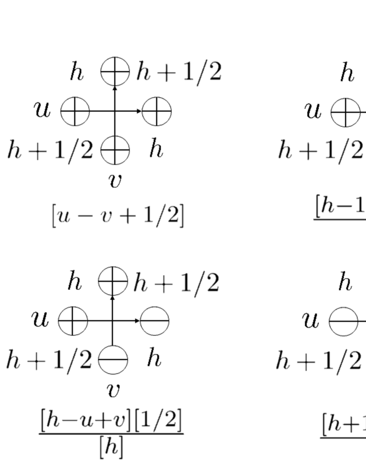
Figure 1: The free-fermionic dynamical $R$-matrix $R_{ab}(u,v|h)$, (3.1). Each line is to be regarded as a representation space and carries a spectral parameter. In this picture, the horizontal lines carry a spectral parameter $u$, while the vertical lines carry $v$. The height variables of neighboring regions (regions separated by a line) differ by 1/2. For the case of the free-fermion model, we can think that the regions take height variables either $h$ or $h+1/2$, due to the property of the dynamical $R$-matrix $R(u,v|h+1)=R(u,v|h)$. The (dual) basis vector $|0\rangle$ ($\langle 0|$) is depicted as $\oplus$, while $|1\rangle$ ($\langle 1|$) is depicted as $\ominus$.

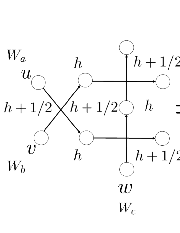
Figure 2: The free-fermionic dynamical Yang–Baxter relation (3.3). The left- and right-hand sides of the figure represent the left- and right-hand sides of the Yang-Baxter relation $R_{bc}(v,w|h)R_{ac}(u,w|h+1/2)R_{ab}(u,v|h)$ and $R_{ab}(u,v|h+1/2)R_{ac}(u,w|h)R_{bc}(v,w|h+1/2)$, respectively.

The dynamical $R$-matrix (3.1) satisfies the dynamical Yang–Baxter relation (Fig. 2)

$$R_{bc}(v,w|h)R_{ac}(u,w|h+1/2)R_{ab}(u,v|h)$$ (3.2)

$$= R_{ab}(u,v|h+1/2)R_{ac}(u,w|h)R_{bc}(v,w|h+1/2),$$ (3.3)

acting on $W_{a}\otimes W_{b}\otimes W_{c}$.

We also introduce the following off-diagonal $K$-matrix acting on $W_{a}$ (see Fig. 3):

$$K_{a}(u,h)=\begin{pmatrix}0&1\\ 1&0\\ \end{pmatrix},$$ (3.4)

One can easily check that the $K$-matrix (3.4) together with the dynamical $R$-matrix (3.1) satisfy the relation

$$R_{ba}(u-v,h)K_{b}(u,h)R_{ab}(v+u,h)K_{a}(v,h)=K_{a}(v,h)R_{ba}(u+v,h)K_{b}(u,h)R_{ab}(u-v,h),$$ (3.5)

which is called the reflection equation or the boundary Yang–Baxter equation [68] (Fig. 4). The reflection equation ensures integrability at the boundary. This off-diagonal $K$-matrix was used as local pieces of the partition functions for the case of the $U_{q}(sl_{2})$ six-vertex model by Kuperberg [12]. We also use this $K$-matrix for the elliptic integrable model in this paper. It seems that it is hard or maybe impossible to extract the off-diagonal $K$-matrix (3.4) from the general full $K$-matrices of elliptic integrable models [69, 70, 71, 72]. This $K$-matrix was used to impose the antiperiodic boundary condition on the ABF model in the paper by Felder-Schorr [65, 73], in which they analyzed the antiperiodic boundary condition by the quantum separation of variables method.

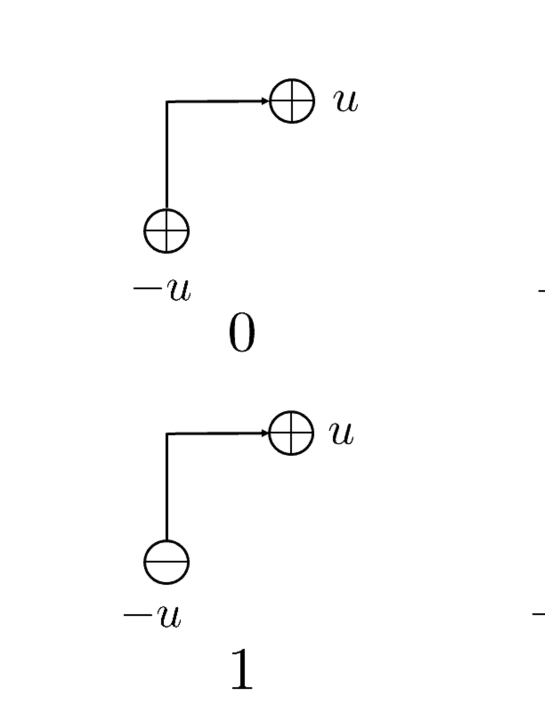
Figure 3: The off-diagonal $K$-matrix $K(u,h)$, (3.4). The horizontal lines carry a spectral parameter $u$, while the vertical lines carry $-u$.

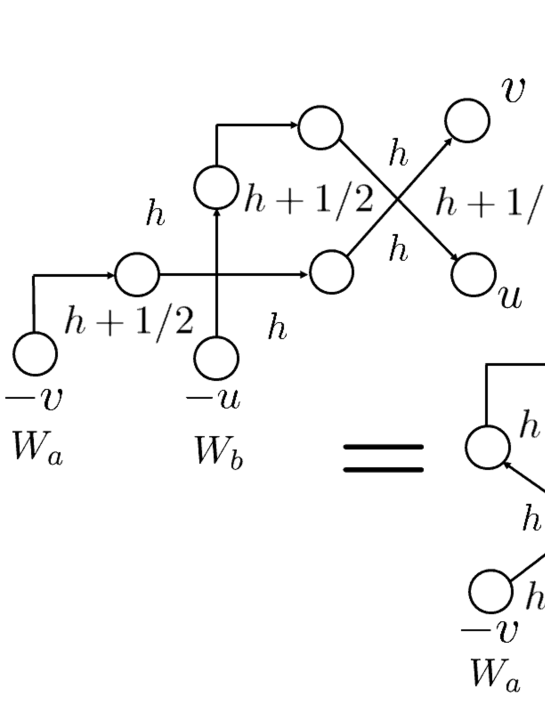
Figure 4: The reflection equation (3.5). The left- and right-hand sides of the figure represent the left- and right-hand sides of the reflection equation $R_{ba}(u-v,h)K_{b}(u,h)R_{ab}(v+u,h)K_{a}(v,h)$ and $K_{a}(v,h)R_{ba}(u+v,h)K_{b}(u,h)R_{ab}(u-v,h)$, respectively.

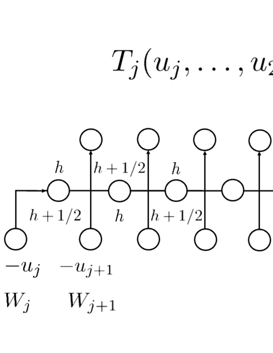
Figure 5: The monodromy matrix $T_{j}(u_{j},\dots,u_{2n}|h)$, (4.3), constructed from one $K$-matrix (3.4) and $2n-j$ dynamical $R$-matrices (3.1) .

4 Partition functions with OS boundary

In this section, we introduce and analyze the partition functions of the free-fermionic face model with OS boundary.

Let us denote the orthonormal basis of $W_{a}$ and its dual by $\{|0\rangle_{a},|1\rangle_{a}\}$ and $\{{}_{a}\langle 0|,{}_{a}\langle 1|\}$. Next, the Pauli spin operators $\sigma^{+}$ and $\sigma^{-}$ are defined as operators acting on the (dual) orthonormal basis as

$$\sigma^{+}|1\rangle =|0\rangle, \sigma^{+}|0\rangle =0, \langle 0|\sigma^{+} =\langle 1|, \langle 1|\sigma^{+} =0,$$ (4.1)

$$\sigma^{-}|0\rangle =|1\rangle, \sigma^{-}|1\rangle =0, \langle 1|\sigma^{-} =\langle 0|, \langle 0|\sigma^{-} =0.$$ (4.2)

To formulate the wavefunctions with a triangular boundary, we introduce the tensor product of the Fock spaces: $W_{1}\otimes\cdots\otimes W_{2n}$.

Using the dynamical $R$-matrix (3.1) and the $K$-matrix (3.4), we next define a monodromy matrix $T_{j}(u_{j},\dots,u_{2n}|h)$, $j=1,\dots,2n$, as

$$T_{j}(u_{j},\dots,u_{2n}|h)=\prod_{k=j+1}^{2n}R_{jk}(u_{j},-u_{k}|h+1/4+(-1)^{k-j}/4)K_{j}(u_{j}),$$ (4.3)

which acts on $W_{j}\otimes\cdots\otimes W_{2n}$. See Fig. 5 for a pictorial depiction of (4.3). Using this monodromy matrix, we introduce the partition functions $P_{2n}(u_{1},\dots,u_{2n}|h)$ as follows (Fig. 6) :

$$P_{2n}(u_{1},\dots,u_{2n},h)={}_{2n}\langle\Omega|T_{2n}(u_{2n}|h)\cdots T_{1}(u_{1},\dots,u_{2n}|h)|\Omega\rangle_{2n},$$ (4.4)

where the states ${}_{2n}\langle\Omega|$ and $|\Omega\rangle_{2n}$ are defined as

$${}_{2n}\langle\Omega|={}_{1}\langle 0|\otimes\cdots\otimes{}_{2n}\langle 0|,$$ (4.5)

$$|\Omega\rangle_{2n}=|0\rangle_{1}\otimes\cdots\otimes|0\rangle_{2n}.$$ (4.6)

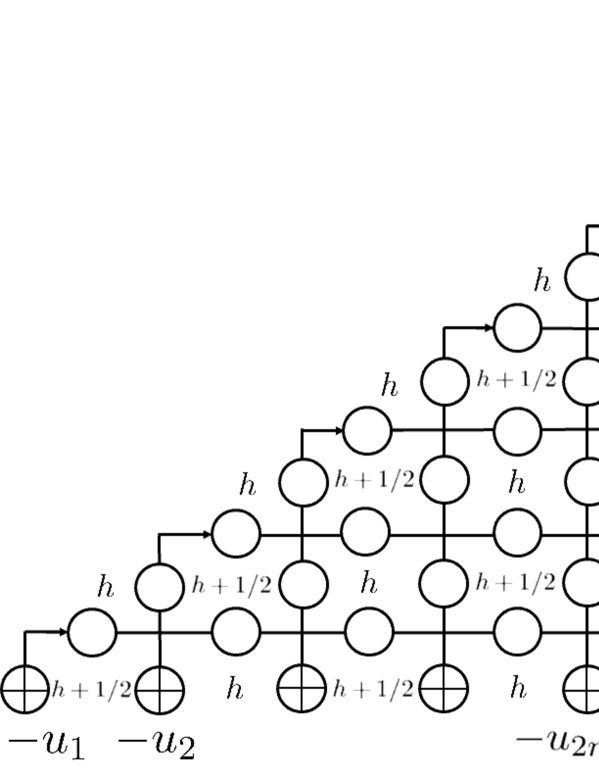
Figure 6: Partition functions $P_{2n}(u_{1},\dots,u_{2n}|h)$, (4.4), with OS boundary.

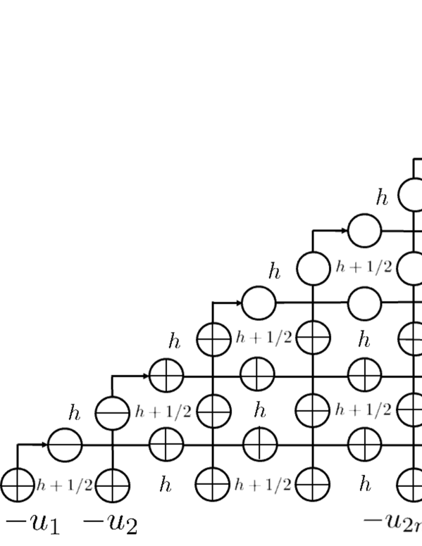
Figure 7: Partition functions $P_{2n}(u_{1},\dots,u_{2n}|h)$ evaluated at $u_{1}=-u_{2}$ (4.9). The bottom two rows are frozen due to the properties of the dynamical $R$-matrix (3.1) and the $K$-matrix (3.4).

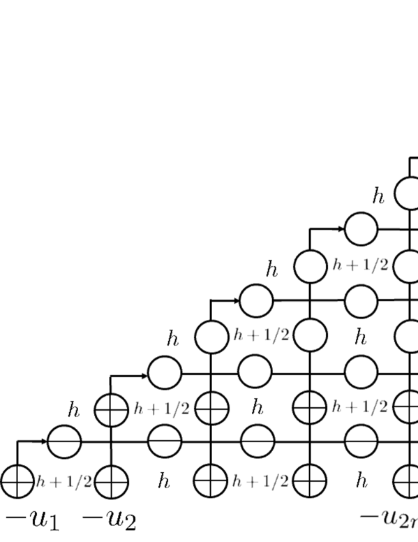
Figure 8: Partition functions $P_{2n}(u_{1},\dots,u_{2n}|h)$ evaluated at $u_{1}=-u_{2n}-1/2$ (4.32). The bottom row and the rightmost column are frozen due to the properties of the dynamical $R$-matrix (3.1) and the $K$-matrix (3.4).

Now we perform the Izergin–Korepin analysis [7, 8] on the partition functions
$P_{2n}(u_{1},\dots,u_{2n}|h)$. The Izergin-Korepin analysis is a technique introduced by Korepin, and the idea is to list the properties of the domain wall boundary partition functions which uniquely determine them, and reduce the problem of explicitly computing the partition functions to that of finding the polynomials satisfying those properties. The Izergin-Korepin technique needs the notion of degree of the polynomial for the uniqueness, and the notion of the degree and the property of the elliptic polynomial stated in Proposition 2.1 in Section 2 ensures the elliptic version of the Izergin-Korepin analysis, which was effectively used for the computation of the ordinary domain wall boundary partition functions of the Andrews-Baxter-Forrester model [29, 30, 31].

Proposition 4.1.

The partition functions with OS boundary $P_{2n}(u_{1},\dots,u_{2n}|h)$ satisfy, and are uniquely determined by, the following properties:

1. The partition functions $P_{2n}(u_{1},\dots,u_{2n}|h)$ are elliptic polynomials in $u_{1}$ of degree $2n-1$ with the following quasi-periodicities:

   $$P_{2n}(u_{1}+1,\dots,u_{2n}|h)=(-1)^{2n-1}P_{2n}(u_{1},\dots,u_{2n}|h),$$ (4.7)

   $$P_{2n}(u_{1}-i\log({\bf q})/\pi,\dots,u_{2n}|h)$$

   $$={} (-{\bf q}^{-1})^{2n-1}\exp\!\Bigg{(}-2\pi i\Bigg{(}(2n-1)u_{1}+h+\sum_{j=2}^{2n}u_{j}\Bigg{)}\Bigg{)}P_{2n}(u_{1},\dots,u_{2n}|h).$$ (4.8)

2. The following relations among the partition functions hold (Fig. 7):

   $$P_{2n}(u_{1},\dots,u_{2n}|h)|_{u_{1}=-u_{\ell}}$$

   $$={} [1/2]\prod_{\begin{subarray}{c}j=2\\ j\neq\ell\end{subarray}}^{2n}[u_{j}+u_{\ell}+1/2][u_{j}-u_{\ell}+1/2]P_{2n-2}(u_{2},\dots,\hat{u_{\ell}},\dots,u_{2n}|h),$$ (4.9)

   for $\ell=2,\dots,2n$, and $\hat{u_{\ell}}$ in $P_{2n-2}(u_{2},\dots,\hat{u_{\ell}},\dots,u_{2n}|h)$ means that $\hat{u_{\ell}}$ is removed.

3. The following evaluation holds:

   $$P_{2}(u_{1},u_{2}|h)=\frac{[1/2][h+u_{1}+u_{2}]}{[h]}.$$ (4.10)

Proof.

Before going into the details of proving Properties (1)–(3), let us first point out that they uniquely determine the partition functions $P_{2n}(u_{1},\dots,u_{2n}|h)$. The uniqueness follows by using induction on $n$, together with the recurrence of Property (2) and the initial condition of Property (3). Property (2) connects $2n-1$ special points $u_{1}=-u_{\ell}$, $\ell=2,\dots,2n$ of $P_{2n}(u_{1},\dots,u_{2n}|h)$ with $P_{2n-2}(u_{2},\dots,\hat{u_{\ell}},\dots,u_{2n}|h)$. These evaluations at $2n-1$ special points and Property (1) together with Proposition 2.1 imply that $P_{2n}(u_{1},\dots,u_{2n}|h)$ is uniquely determined from $P_{2n-2}(u_{2},\dots,\hat{u_{\ell}},\dots,u_{2n}|h)$ by Properties (1) and (2). Property (3) corresponds to the initial term of the recurrence relation.

Now let us go into the details of the proof. Properties (1)–(3) can be proved in the standard way.

We first show Property (1). We use the completeness relation in one up-spin sector,

$$\sum_{j=1}^{2n-1}|0^{j-1}10^{2n-j-1}\rangle\langle 0^{j-1}10^{2n-j-1}|=\mathrm{Id},$$ (4.11)

on the space $W_{2}\otimes\cdots\otimes W_{2n}$ with

$$|0^{j-1}10^{2n-j-1}\rangle =|0\rangle_{2}\otimes\cdots\otimes|0\rangle_{j}\otimes|1\rangle_{j+1}\otimes|0\rangle_{j+2}\otimes\cdots\otimes|0\rangle_{2n},$$

$$\langle 0^{j-1}10^{2n-j-1}| ={}_{2}\langle 0|\otimes\cdots\otimes{}_{j}\langle 0|\otimes{}_{j+1}\langle 1|\otimes{}_{j+2}\langle 0|\otimes\cdots\otimes{}_{2n}\langle 0|,$$

and decompose $P_{2n}(u_{1},\dots,u_{2n}|h)$ as

$$P_{2n}(u_{1},\dots,u_{2n}|h)$$

$$={} \sum_{j=1}^{2n-1}{}_{2n-1}\langle\Omega|T_{2n}(u_{2n}|h)\cdots T_{2}(u_{2},\dots,u_{2n}|h)|0^{j-1}10^{2n-j-1}\rangle$$

$$\times{}_{1}\langle 0|\otimes\langle 0^{j-1}10^{2n-j-1}|T_{1}(u_{1},\dots,u_{2n}|h)|\Omega\rangle_{2n},$$ (4.12)

where ${}_{2n-1}\langle\Omega|={}_{2}\langle 0|\otimes\cdots\otimes{}_{2n}\langle 0|$.

One can easily calculate the explicit forms of ${}_{1}\langle 0|\otimes\langle 0^{j-1}10^{2n-j-1}|T_{1}(u_{1},\dots,u_{2n}|h)|\Omega\rangle_{2n}:=f_{j}(u_{1})$ in (4.12), which are

$$f_{j}(u_{1})={} \frac{[1/2][h+(j-1)/2+u_{1}+u_{j+1}]}{[h]}$$

$$\times\prod_{k=2}^{j}[u_{1}+u_{k}]\prod_{k=j+2}^{2n}[u_{1}+u_{k}+1/2].$$ (4.13)

It is easy to see from (4.13) and the quasi-periodicities of the theta functions (2.5) and (2.6) that the quasi-periodicities of $f_{j}(u_{1})$ are

$$f_{j}(u_{1}+1)=(-1)^{2n-1}f_{j}(u_{1}),$$ (4.14)

$$f_{j}(u_{1}-i\log({\bf q})/\pi)$$

$$={} (-{\bf q}^{-1})^{2n-1}\exp\!\Bigg{(}-2\pi i\Bigg{(}(2n-1)u_{1}+h+\sum_{\ell=2}^{2n}u_{\ell}\Bigg{)}\Bigg{)}f_{j}(u_{1}).$$ (4.15)

Since the quasi-periodicities for $f_{j}(u_{1})$, (4.14), and (4.15), do not depend on $j$, and noting that the dependence on $u_{1}$ for each summand in the right hand side of (4.12), comes only from $f_{j}(u_{1})$, one finds that the quasi-periodicities of the partition functions $P_{2n}(u_{1},\dots,u_{2n}|h)$ are given by (4.7) and (4.8). One also concludes from (4.7) and (4.8) that $P_{2n}(u_{1},\dots,u_{2n}|h)$ are elliptic polynomials in $u_{1}$ of degree $2n-1$.

Next, we prove property (2). First, one shows (4.9) for the case $\ell=2$ by using a graphical representation of the partition functions (Fig. 7), as is always the case when using the Korepin’s method. First, one observes that the $K$-matrix at the bottom row is already frozen since the $K$-matrix we use for the partition fuctions $P_{2n}(u_{1},\dots,u_{2n}|h)$ is an off-diagonal one (3.4). If we set $u_{1}=-u_{2}$, one finds that the $R$-matrix adjacent to the frozen $K$-matrix gets frozen since ${}_{1}\langle 1|{}_{2}\langle 0|R_{12}(-u_{2},-u_{2},h)|1\rangle_{1}|0\rangle_{2}=0$, and continuing graphical observation using the ice-rule

$${}_{a}\langle\gamma|{}_{b}\langle\delta|R_{ab}(u,v,h)|\alpha\rangle_{a}|\beta\rangle_{b}=0,\qquad\text{unless}\quad\alpha+\beta=\gamma+\delta,$$ (4.16)

one sees that the two bottom rows freeze (Fig. 7). The product of the matrix elements of the $R$-matrices of the frozen two rows is $\displaystyle[1/2]\prod_{j=3}^{2n}[u_{j}+u_{2}+1/2][u_{j}-u_{2}+1/2]$, and the remaining unfrozen part is $P_{2n-2}(u_{3},\dots,u_{2n}|h)$, and we get

$$P_{2n}(u_{1},\dots,u_{2n}|h)|_{u_{1}=-u_{2}}$$

$$={} [1/2]\prod_{j=3}^{2n}[u_{j}+u_{2}+1/2][u_{j}-u_{2}+1/2]P_{2n-2}(u_{3},\dots,u_{2n}|h).$$ (4.17)

One can show that the partition functions $P_{2n}(u_{1},\dots,u_{2n}|h)$ are symmetric with respect to the spectral parameters $u_{1},\dots,u_{2n}$ by the standard railroad argument using the dynamical Yang-Baxter relation and the reflection equation (Kuperberg [12], see also [63]). From (4.17) and the symmetry property, one finds that (4.9) holds.

Finally, it is trivial to check Property (3) from the definition of the $R$-matrix (3.1).

∎

One can prove that there are explicit expressions for the partition functions with OS boundary $P_{2n}(u_{1},\dots,u_{2n}|h)$ in terms of elliptic Pfaffians by showing that the right hand side of (4.18) satisfies all the properties in Proposition 4.1.

Theorem 4.2.

The partition functions with OS boundary $P_{2n}(u_{1},\dots,u_{2n}|h)$ have the following expressions using elliptic Pfaffians:

$$P_{2n}(u_{1},\dots,u_{2n}|h)$$

$$= \prod_{1\leq i<j\leq 2n}\frac{[u_{j}+u_{i}][u_{j}-u_{i}+1/2]}{[u_{j}-u_{i}]}\mathrm{Pf}\Bigg{(}\frac{[1/2][u_{j}-u_{i}][u_{i}+u_{j}+h]}{[h][u_{i}+u_{j}][u_{j}-u_{i}+1/2]}\Bigg{)}_{1\leq i,j\leq 2n}.$$ (4.18)

Note that $\displaystyle\Bigg{(}\frac{[1/2][u_{j}-u_{i}][u_{i}+u_{j}+h]}{[h][u_{i}+u_{j}][u_{j}-u_{i}+1/2]}\Bigg{)}_{1\leq i,j\leq 2n}$ is a skew-symmetric matrix which can be checked using the facts that $[u]$ is an odd function and the property (2.7).

Proof.

Let us denote the right hand side of (4.18) as $E_{2n}(u_{1},\dots,u_{2n}|h)$:

$$E_{2n}(u_{1},\dots,u_{2n}|h)$$

$$:= \prod_{1\leq i<j\leq 2n}\frac{[u_{j}+u_{i}][u_{j}-u_{i}+1/2]}{[u_{j}-u_{i}]}\mathrm{Pf}\Bigg{(}\frac{[1/2][u_{j}-u_{i}][u_{i}+u_{j}+h]}{[h][u_{i}+u_{j}][u_{j}-u_{i}+1/2]}\Bigg{)}_{1\leq i,j\leq 2n}.$$ (4.19)

We show that $E_{2n}(u_{1},\dots,u_{2n}|h)$ satisfies all the properties in Proposition 4.1. Let us show Property (1). To check this, we view $E_{2n}(u_{1},\dots,u_{2n}|h)$ as a function of $u_{1}$ and split the function as $E_{2n}(u_{1},\dots,u_{2n}|h)=e_{1}(u_{1})e_{2}(u_{1})$, where $e_{1}(u_{1})$ and $e_{2}(u_{1})$ are the overall factor and the elliptic Pfaffian, respectively

$$e_{1}(u_{1}) =\prod_{1\leq i<j\leq 2n}\frac{[u_{j}+u_{i}][u_{j}-u_{i}+1/2]}{[u_{j}-u_{i}]},$$ (4.20)

$$e_{2}(u_{1}) =\mathrm{Pf}\Bigg{(}\frac{[1/2][u_{j}-u_{i}][u_{i}+u_{j}+h]}{[h][u_{i}+u_{j}][u_{j}-u_{i}+1/2]}\Bigg{)}_{1\leq i,j\leq 2n}.$$ (4.21)

Using the quasi-periodicities of the theta functions (2.5) and (2.6), it is easy to calculate the quasi-periodicites of the overall factor $e_{1}(u_{1})$:

$$e_{1}(u_{1}+1)=(-1)^{2n-1}e_{1}(u_{1}),$$ (4.22)

$$e_{1}(u_{1}-i\log({\bf q})/\pi)$$

$$={} (-{\bf q}^{-1})^{2n-1}\exp\!\Bigg{(}-2\pi i\Bigg{(}(2n-1)u_{1}+\sum_{j=2}^{2n}u_{j}-1/2\Bigg{)}\Bigg{)}e_{1}(u_{1}).$$ (4.23)

Next, noting that the quasi-periodicities of the matrix elements of the first row of the matrix $\displaystyle X=\Bigg{(}\frac{[1/2][u_{j}-u_{i}][u_{i}+u_{j}+h]}{[h][u_{i}+u_{j}][u_{j}-u_{i}+1/2]}\Bigg{)}_{1\leq i,j\leq 2n}$ are given by

$$\frac{[1/2][u_{j}-(u_{1}+1)][(u_{1}+1)+u_{j}+h]}{[h][(u_{1}+1)+u_{j}][u_{j}-(u_{1}+1)+1/2]}=\frac{[1/2][u_{j}-u_{1}][u_{1}+u_{j}+h]}{[h][u_{1}+u_{j}][u_{j}-u_{1}+1/2]},$$ (4.24)

$$\frac{[1/2][u_{j}-(u_{1}-i\log({\bf q})/\pi)][(u_{1}-i\log({\bf q})/\pi)+u_{j}+h]}{[h][(u_{1}-i\log({\bf q})/\pi)+u_{j}][u_{j}-(u_{1}-i\log({\bf q})/\pi)+1/2]}$$

$$=\exp(-2\pi i(h+1/2))\frac{[1/2][u_{j}-u_{1}][u_{1}+u_{j}+h]}{[h][u_{1}+u_{j}][u_{j}-u_{1}+1/2]},$$ (4.25)

and using the definition of the Pfaffian of a matrix (2.1), one can calculate the quasi-periodicities of $e_{2}(u_{1})=\mathrm{Pf}X$ and get

$$e_{2}(u_{1}+1)=e_{2}(u_{1}),$$ (4.26)

$$e_{2}(u_{1}-i\log({\bf q})/\pi)=\exp(-2\pi i(h+1/2))e_{2}(u_{1}).$$ (4.27)

Combining (4.22), (4.23), (4.26) and (4.27), we get the quasi-periodicities of $E_{2n}(u_{1},\dots,u_{2n}|h)$

$$E_{2n}(u_{1}+1,\dots,u_{2n}|h)=(-1)^{2n-1}E_{2n}(u_{1},\dots,u_{2n}|h),$$ (4.28)

$$E_{2n}(u_{1}-i\log({\bf q})/\pi,\dots,u_{2n}|h)$$

$$={} (-{\bf q}^{-1})^{2n-1}\exp\!\Bigg{(}-2\pi i\Bigg{(}(2n-1)u_{1}+h+\sum_{j=2}^{2n}u_{j}\Bigg{)}\Bigg{)}E_{2n}(u_{1},\dots,u_{2n}|h).$$ (4.29)

We can also check that $E_{2n}(u_{1}+1,\dots,u_{2n}|h)$ is holomorphic as a function of $u_{1}$. The factors $[u_{i}+u_{j}]$ and $[u_{j}-u_{i}+1/2]$ in the denominators of $\displaystyle X_{ij}=\frac{[1/2][u_{j}-u_{i}][u_{i}+u_{j}+h]}{[h][u_{i}+u_{j}][u_{j}-u_{i}+1/2]}$, the matrix elements of $X$ which are used to construct the Pfaffian, are cancelled by the overall factor $\displaystyle\prod_{1\leq i<j\leq 2n}\frac{[u_{j}+u_{i}][u_{j}-u_{i}+1/2]}{[u_{j}-u_{i}]}$. The factors $[u_{k}-u_{1}]$, $k=2,\dots,2n$ in the denominator of the overall factor $\displaystyle\prod_{1\leq i<j\leq 2n}\frac{[u_{j}+u_{i}][u_{j}-u_{i}+1/2]}{[u_{j}-u_{i}]}$ may lead to singularities at $u_{1}=u_{k}\ (k=2,\dots,2n)$, but do not. For example, let us see the case $k=2$. If one expands the Pfaffian of the matrix $X$, all summands containing $X_{12}$ as a factor of the product have the factor $[u_{2}-u_{1}]$ in the numerator. The sum of the summands which do not contain $X_{12}$ can be rearranged as a linear combination of the terms $(X_{1j}X_{2k}-X_{1k}X_{2j})\prod_{\ell=3}^{n}X_{\sigma^{\prime}(2\ell-1)\sigma^{\prime}(2\ell)}\ (j,k\neq 1,2,\ \sigma^{\prime}\in M_{2n-4})$, all of which vanish at $u_{1}=u_{2}$. Hence, we find $E_{2n}(u_{1},\dots,u_{2n}|h)$ is an elliptic polynomial of degree $2n-1$ and we find Property (1) holds.

Next, let us show Property (2). Applying the expansion formula for the Pfaffian (2.3) to the matrix $X$, $E_{2n}(u_{1},\dots,u_{2n}|h)$ can be expanded as

$$E_{2n}(u_{1},\dots,u_{2n}|h)$$

$$= \prod_{1\leq i<j\leq 2n}\frac{[u_{j}+u_{i}][u_{j}-u_{i}+1/2]}{[u_{j}-u_{i}]}\sum_{k=2}^{2n}\frac{[1/2][u_{k}-u_{1}][u_{1}+u_{k}+h]}{[h][u_{1}+u_{k}][u_{k}-u_{1}+1/2]}\mathrm{Pf}X_{1,k}^{1,k}.$$ (4.30)

Then one notes that if one substitutes $u_{1}=-u_{\ell}$, only the summand $k=\ell$ of the sum in the right hand side of (4.30) survives. Here, we use the basic property for the theta function $[0]=0$ for this observation. After the substitution $u_{1}=-u_{\ell}$ in (4.30) and after simplifications, one finds

$$E_{2n}(u_{1},\dots,u_{2n}|h)|_{u_{1}=-u_{\ell}}$$

$$= [1/2]\prod_{\begin{subarray}{c}j=2\\ j\neq\ell\end{subarray}}^{2n}[u_{j}+u_{\ell}+1/2][u_{j}-u_{\ell}+1/2]\prod_{\begin{subarray}{c}1\leq i<j\leq 2n\\ i,j\neq 1,\ell\end{subarray}}\frac{[u_{j}+u_{i}][u_{j}-u_{i}+1/2]}{[u_{j}-u_{i}]}\mathrm{Pf}X_{1,\ell}^{1,\ell},$$

$$={} [1/2]\prod_{\begin{subarray}{c}j=2\\ j\neq\ell\end{subarray}}^{2n}[u_{j}+u_{\ell}+1/2][u_{j}-u_{\ell}+1/2]E_{2n-2}(u_{2},\dots,\hat{u_{\ell}},\dots,u_{2n}|h).$$ (4.31)

Here, we have used the fact that $[u]$ is odd $[-u]=-[u]$ and the property (2.7) to get the expression (4.31) from the expansion (4.30). Hence Property (2) is proved.

The only thing left to do is to check Property (3), which can be easily seen from the definition of $E_{2n}(u_{1},\dots,u_{2n}|h)$ (4.19). ∎

We can make another Proposition (Korepin’s characterization of the partition functions) which looks almost the same, but is slightly different from Proposition 4.1, i.e., a different version of the elliptic Izergin-Korepin analysis which is presented below.

Proposition 4.3.

The partition functions with OS boundary $P_{2n}(u_{1},\dots,u_{2n}|h)$ satisfy Properties (1) and (3) of Proposition 4.1, together with:
The following relations among the partition functions hold (Fig. 8):

$$P_{2n}(u_{1},\dots,u_{2n}|h)|_{u_{1}=-u_{\ell}-1/2}$$

$$={} \frac{[h-1/2][1/2]}{[h]}\prod_{\begin{subarray}{c}j=2\\ j\neq\ell\end{subarray}}^{2n}[u_{j}+u_{\ell}][u_{j}-u_{\ell}-1/2]P_{2n-2}(u_{2},\dots,\hat{u_{\ell}},\dots,u_{2n}|h),$$ (4.32)

for $\ell=2,\dots,2n$, and $\hat{u_{\ell}}$ in $P_{2n-2}(u_{2},\dots,\hat{u_{\ell}},\dots,u_{2n}|h)$ means that $\hat{u_{\ell}}$ is removed.

Proof.

The only additional thing to prove is (4.32). It is enough to prove the case $\ell=2n$ since the other cases $\ell=2,\dots,2n-1$ follow from the case $\ell=2n$ of (4.32) by using the symmetry of $P_{2n}(u_{1},\dots,u_{2n}|h)$ with respect to the variables $u_{1},\dots,u_{2n}$.

We again use the graphical representation of $P_{2n}(u_{1},\dots,u_{2n}|h)$ (Fig. 8). We first realize that when we set $u_{1}$ to $u_{1}=-u_{2n}-1/2$, the $R$-matrix at the southeast corner starts to freeze since ${}_{1}\langle 0|{}_{2n}\langle 0|R_{1,2n}(-u_{2n}-1/2,-u_{2n},h)|0\rangle_{1}|0\rangle_{2n}=0$, and continuing graphical observation using the ice-rule of the $R$-matrix (4.16), one finds that the $R$- and $K$-matrices at the bottom row and the rightmost column are frozen. The contribution of these frozen parts to the partition functions is the overall factor $\displaystyle[h-1/2][1/2][h]^{-1}\prod_{j=2}^{2n-1}[u_{j}+u_{2n}][u_{j}-u_{2n}-1/2]$, and the remaining unfrozen part is $P_{2n-2}(u_{2},\dots,u_{2n-1}|h)$. Hence, we get

$$P_{2n}(u_{1},\dots,u_{2n}|h)|_{u_{1}=-u_{2n}-1/2}$$

$$= \frac{[h-1/2][1/2]}{[h]}\prod_{j=2}^{2n-1}[u_{j}+u_{2n}][u_{j}-u_{2n}-1/2]P_{2n-2}(u_{2},\dots,u_{2n-1}|h).$$ (4.33)

∎

One can obtain an elliptic Pfaffian representation of the partition functions which is similar to that of (4.18) in Theorem 4.2 by finding a representation satisfying the properties in Proposition 4.3.

Theorem 4.4.

The partition functions $P_{2n}(u_{1},\dots,u_{2n}|h)$ with OS boundary have the following expressions using elliptic Pfaffians:

$$P_{2n}(u_{1},\dots,u_{2n}|h)$$

$$= \prod_{1\leq i<j\leq 2n}\frac{[u_{j}+u_{i}+1/2][u_{j}-u_{i}+1/2]}{[u_{j}-u_{i}]}\mathrm{Pf}\Bigg{(}\frac{[1/2][u_{j}-u_{i}][u_{i}+u_{j}+h]}{[h][u_{i}+u_{j}+1/2][u_{j}-u_{i}+1/2]}\Bigg{)}_{1\leq i,j\leq 2n}.$$ (4.34)

Proof.

This can be proved in the same way as proving Theorem 4.2. For example, one can show that the RHS of (4.34) satisfies (4.32) in the same way as proving that the RHS of (4.18) satisfies (4.9) using the expansion formula for the Pfaffian (2.3). ∎

We derived two elliptic Pfaffian representations of the partition functions $P_{2n}(u_{1},\dots,u_{2n}|h)$ (4.18) in Theorem 4.2 and (4.34) in Theorem 4.4 based on two versions of the Korepin’s method Proposition 4.1 and Proposition 4.3. By comparing (4.18) and (4.34), we get the following identity between two elliptic Pfaffians.

Theorem 4.5.

The following identity between two elliptic Pfaffians holds:

$$\prod_{1\leq i<j\leq 2n}[u_{j}+u_{i}]\mathrm{Pf}\Bigg{(}\frac{[u_{j}-u_{i}][u_{i}+u_{j}+h]}{[u_{i}+u_{j}][u_{j}-u_{i}+1/2]}\Bigg{)}_{1\leq i,j\leq 2n}$$

$$= \prod_{1\leq i<j\leq 2n}[u_{j}+u_{i}+1/2]\mathrm{Pf}\Bigg{(}\frac{[u_{j}-u_{i}][u_{i}+u_{j}+h]}{[u_{i}+u_{j}+1/2][u_{j}-u_{i}+1/2]}\Bigg{)}_{1\leq i,j\leq 2n}.$$ (4.35)

The special case $h=0$ of the identity (4.35) can be obtained by combining the following two factorization formulas for the elliptic Pfaffians by Rosengren [34, 35] and Rains [36].

$$\mathrm{Pf}\Bigg{(}\frac{[u_{j}-u_{i}]}{[u_{j}-u_{i}+1/2]}\Bigg{)}_{1\leq i,j\leq 2n} =\prod_{1\leq i<j\leq 2n}\frac{[u_{j}-u_{i}]}{[u_{j}-u_{i}+1/2]},$$ (4.36)

$$\mathrm{Pf}\Bigg{(}\frac{[u_{j}-u_{i}][u_{i}+u_{j}]}{[u_{i}+u_{j}+1/2][u_{j}-u_{i}+1/2]}\Bigg{)}_{1\leq i,j\leq 2n} =\prod_{1\leq i<j\leq 2n}\frac{[u_{j}-u_{i}][u_{i}+u_{j}]}{[u_{i}+u_{j}+1/2][u_{j}-u_{i}+1/2]}.$$ (4.37)

See Remark 2.1 in [34] for example where it is explained that (4.36) is a special case of the Pfaffian evaluation by Rosengren ((2.9) and (2.11) in [34]), and (4.37) is a modular dual of the Pfaffian evaluation by Rains (the last equation in Remark 2.1 in [34] and Theorem 2.10 in [36]).

We directly check (4.35) for the case $n=2$ in the Appendix by repeatedly using addition formulas for the theta functions (2.8).

5 Conclusion

In this paper, we studied the partition functions of the elliptic free-fermionic face model with OS boundary, and analyzed them by using the elliptic Izergin-Korepin analysis. We obtained the representations of the partition functions using elliptic Pfaffians. Since we can use the Korepin’s method in two ways, we can get two Pfaffian representations for the same partition functions. As a corollary of the two expressions, we get an identity between two elliptic Pfaffians.

It would be interesting to extend the analysis performed on the OS boundary in this paper to other boundary conditions, i.e., consider various variations of the domain wall boundary partition functions introduced by Kuperberg [12] for the case of the elliptic face models. More complicated boundary conditions may lead to expressions as products of determinants and Pfaffians as is the case for the trigonometric models, and may also lead to various interesting identities between elliptic determinants and elliptic Pfaffians. It would also be interesting to investigate if the elliptic Pfaffian identities by Okada [33], Rosengren [34, 35] and Rains [36] can be understood as different representations of the same partition functions of elliptic integrable models.

Appendix A Appendix: An elemenary proof of (4.35) for the case $n=2$

In this Appendix, we check (4.35) for the case $n=2$ by elementary manipulations. In this case, one can see from the definition of Pfaffians (2.1) that proving (4.35) is equivalent to showing the following identity

$$\frac{[u_{2}-u_{1}][u_{1}+u_{2}+h][u_{4}-u_{3}][u_{3}+u_{4}+h]}{[u_{2}-u_{1}+1/2][u_{4}-u_{3}+1/2]}$$

$$\times[u_{3}+u_{1}+1/2][u_{4}+u_{1}+1/2][u_{3}+u_{2}+1/2][u_{4}+u_{2}+1/2]$$

$$- \frac{[u_{3}-u_{1}][u_{1}+u_{3}+h][u_{4}-u_{2}][u_{2}+u_{4}+h]}{[u_{3}-u_{1}+1/2][u_{4}-u_{2}+1/2]}$$

$$\times[u_{2}+u_{1}+1/2][u_{4}+u_{1}+1/2][u_{3}+u_{2}+1/2][u_{4}+u_{3}+1/2]$$

$$+ \frac{[u_{4}-u_{1}][u_{1}+u_{4}+h][u_{3}-u_{2}][u_{2}+u_{3}+h]}{[u_{4}-u_{1}+1/2][u_{3}-u_{2}+1/2]}$$

$$\times[u_{2}+u_{1}+1/2][u_{3}+u_{1}+1/2][u_{4}+u_{2}+1/2][u_{4}+u_{3}+1/2]$$

$$= \frac{[u_{2}-u_{1}][u_{1}+u_{2}+h][u_{4}-u_{3}][u_{3}+u_{4}+h][u_{3}+u_{1}][u_{4}+u_{1}][u_{3}+u_{2}][u_{4}+u_{2}]}{[u_{2}-u_{1}+1/2][u_{4}-u_{3}+1/2]}$$

$$- \frac{[u_{3}-u_{1}][u_{1}+u_{3}+h][u_{4}-u_{2}][u_{2}+u_{4}+h][u_{2}+u_{1}][u_{4}+u_{1}][u_{3}+u_{2}][u_{4}+u_{3}]}{[u_{3}-u_{1}+1/2][u_{4}-u_{2}+1/2]}$$

$$+ \frac{[u_{4}-u_{1}][u_{1}+u_{4}+h][u_{3}-u_{2}][u_{2}+u_{3}+h][u_{2}+u_{1}][u_{3}+u_{1}][u_{4}+u_{2}][u_{4}+u_{3}]}{[u_{4}-u_{1}+1/2][u_{3}-u_{2}+1/2]}.$$ (A.1)

Let us show this using the addition formula for the theta functions (2.8) repeatedly. The difference between the left hand side and the right hand side of (A.1) can be expressed as

$$\frac{[u_{2}-u_{1}][u_{1}+u_{2}+h][u_{4}-u_{3}][u_{3}+u_{4}+h]}{[u_{2}-u_{1}+1/2][u_{4}-u_{3}+1/2]}$$

$$\times ([u_{3}+u_{1}+1/2][u_{4}+u_{1}+1/2][u_{3}+u_{2}+1/2][u_{4}+u_{2}+1/2]$$

$$-[u_{3}+u_{1}][u_{4}+u_{1}][u_{3}+u_{2}][u_{4}+u_{2}])$$

$$- \frac{[u_{3}-u_{1}][u_{1}+u_{3}+h][u_{4}-u_{2}][u_{2}+u_{4}+h]}{[u_{3}-u_{1}+1/2][u_{4}-u_{2}+1/2]}$$

$$\times ([u_{2}+u_{1}+1/2][u_{4}+u_{1}+1/2][u_{3}+u_{2}+1/2][u_{4}+u_{3}+1/2]$$

$$-[u_{2}+u_{1}][u_{4}+u_{1}][u_{3}+u_{2}][u_{4}+u_{3}])$$

$$+ \frac{[u_{4}-u_{1}][u_{1}+u_{4}+h][u_{3}-u_{2}][u_{2}+u_{3}+h]}{[u_{4}-u_{1}+1/2][u_{3}-u_{2}+1/2]}$$

$$\times ([u_{2}+u_{1}+1/2][u_{3}+u_{1}+1/2][u_{4}+u_{2}+1/2][u_{4}+u_{3}+1/2]$$

$$-[u_{2}+u_{1}][u_{3}+u_{1}][u_{4}+u_{2}][u_{4}+u_{3}]).$$ (A.2)

Using the addition formula for the theta functions (2.8) (and (2.7)), one finds

$$[u_{3}+u_{1}+1/2][u_{4}+u_{1}+1/2][u_{3}+u_{2}+1/2][u_{4}+u_{2}+1/2]$$

$$-[u_{3}+u_{1}][u_{4}+u_{1}][u_{3}+u_{2}][u_{4}+u_{2}]$$

$$= [1/2][u_{1}+u_{2}+u_{3}+u_{4}+1/2][u_{2}-u_{1}+1/2][u_{4}-u_{3}+1/2],$$ (A.3)

$$[u_{2}+u_{1}+1/2][u_{4}+u_{1}+1/2][u_{3}+u_{2}+1/2][u_{4}+u_{3}+1/2]$$

$$-[u_{2}+u_{1}][u_{4}+u_{1}][u_{3}+u_{2}][u_{4}+u_{3}]$$

$$= [1/2][u_{1}+u_{2}+u_{3}+u_{4}+1/2][u_{3}-u_{1}+1/2][u_{4}-u_{2}+1/2],$$ (A.4)

$$[u_{2}+u_{1}+1/2][u_{3}+u_{1}+1/2][u_{4}+u_{2}+1/2][u_{4}+u_{3}+1/2]$$

$$-[u_{2}+u_{1}][u_{3}+u_{1}][u_{4}+u_{2}][u_{4}+u_{3}]$$

$$= [1/2][u_{1}+u_{2}+u_{3}+u_{4}+1/2][u_{3}-u_{2}+1/2][u_{4}-u_{1}+1/2].$$ (A.5)

Using the identities (A.3), (A.4) and (A.5), (A.2) reduces to

$$\frac{[u_{2}-u_{1}][u_{1}+u_{2}+h][u_{4}-u_{3}][u_{3}+u_{4}+h]}{[u_{2}-u_{1}+1/2][u_{4}-u_{3}+1/2]}$$

$$\times [1/2][u_{1}+u_{2}+u_{3}+u_{4}+1/2][u_{2}-u_{1}+1/2][u_{4}-u_{3}+1/2]$$

$$- \frac{[u_{3}-u_{1}][u_{1}+u_{3}+h][u_{4}-u_{2}][u_{2}+u_{4}+h]}{[u_{3}-u_{1}+1/2][u_{4}-u_{2}+1/2]}$$

$$\times [1/2][u_{1}+u_{2}+u_{3}+u_{4}+1/2][u_{3}-u_{1}+1/2][u_{4}-u_{2}+1/2]$$

$$+ \frac{[u_{4}-u_{1}][u_{1}+u_{4}+h][u_{3}-u_{2}][u_{2}+u_{3}+h]}{[u_{4}-u_{1}+1/2][u_{3}-u_{2}+1/2]}$$

$$\times [1/2][u_{1}+u_{2}+u_{3}+u_{4}+1/2][u_{3}-u_{2}+1/2][u_{4}-u_{1}+1/2]$$

$$= [1/2][u_{1}+u_{2}+u_{3}+u_{4}+1/2]([u_{2}-u_{1}][u_{1}+u_{2}+h][u_{4}-u_{3}][u_{3}+u_{4}+h]$$

$$- [u_{3}-u_{1}][u_{1}+u_{3}+h][u_{4}-u_{2}][u_{2}+u_{4}+h]+[u_{4}-u_{1}][u_{1}+u_{4}+h][u_{3}-u_{2}][u_{2}+u_{3}+h]).$$ (A.6)

One can apply the addition formula (2.8) again to get

$$[u_{2}-u_{1}][u_{1}+u_{2}+h][u_{4}-u_{3}][u_{3}+u_{4}+h]-[u_{3}-u_{1}][u_{1}+u_{3}+h][u_{4}-u_{2}][u_{2}+u_{4}+h]$$

$$+ [u_{4}-u_{1}][u_{1}+u_{4}+h][u_{3}-u_{2}][u_{2}+u_{3}+h]=0,$$ (A.7)

and we find the right hand side of (A.6) becomes zero. Hence (4.35) for the case $n=2$ is proved.

References

- [1] Bethe, H.: On the theory of metals. I. Eigenvalues and eigenfunctions of a linear chain of atoms. Z. Phys. 71, 205-226 (1931)
- [2] Faddeev, L.D., Sklyanin, E.K., Takhtajan, L.A.: Quantum inverse problem method I. Theor. Math. Phys. 40, 194-220 (1979)
- [3] Baxter, R.J.: Exactly Solved Models in Statistical Mechanics. Academic Press, London (1982)
- [4] Korepin, V.B., Bogoliubov, N.M., Izergin, A.G.: Quantum Inverse Scattering Method and Correlation Functions. Cambridge University Press, Cambridge (1993).
- [5] Jimbo, M., Miwa, T.: Algebraic Analysis of Solvable Lattice Models. American Mathematical Society, Providence (1995)
- [6] Reshetikhin, N.: Lectures on integrable models in statistical mechanics. In: Exact Methods in Low- Dimensional Statistical Physics and Quantum Computing, Proceedings of Les Houches School in Theoretical Physics. Oxford University Press (2010)
- [7] Korepin, V.E.: Calculation of norms of Bethe wave functions. Commun. Math. Phys. 86, 391-418 (1982)
- [8] Izergin, A.: Partition function of the six-vertex model in a finite volume. Sov. Phys. Dokl. 32, 878-879 (1987)
- [9] Tsuchiya, O.: Determinant formula for the six-vertex model with reflecting end. J. Math. Phys. 39, 5946-5951 (1998)
- [10] Bressoud, D.: Proofs and Confirmations: The Story of the Alternating Sign Matrix Conjecture. MAA Spectrum, Mathematical Association of America, Washington, DC (1999)
- [11] Kuperberg, G.: Another proof of the alternating-sign matrix conjecture. Int. Math. Res. Not. 3, 139-150 (1996)
- [12] Kuperberg, G.: Symmetry classes of alternating-sign matrices under one roof. Ann. Math. 156, 835-866 (2002)
- [13] Okada, S.: Enumeration of symmetry classes of alternating sign matrices and characters of classical groups. J. Alg. Comb. 23, 43-69 (2001)
- [14] Razumov, A.V., Stroganov, Y.G.: On refined enumerations of some symmetry classes of ASMs. Theor. Math. Phys. 141, 1609-1630 (2004)
- [15] Colomo, F., Pronko, A.G.: Square ice, alternating sign matrices, and classical orthogonal polynomials. J. Stat. Mech.: Theor. Exp. P01005 (2005)
- [16] Betea, D., Wheeler, M., Zinn-Justin, P.: Refined Cauchy/Littlewood identities and six-vertex model partition functions: II. Proofs and new conjectures. J. Alg. Combinatorics. 42, 555-603 (2015)
- [17] Behrend, R.E., Fischer, I., Konvalinka, M.: Diagonally and antidiagonally symmetric alternating sign matrices of odd order: Adv. Math. 315, 324-365 (2017)
- [18] Okada, S.: Alternating sign matrices and some deformations of Weyl’s denominator formula. J. Algebraic Comb. 2, 155-176 (1993)
- [19] Hamel, A., King, R.C.: Symplectic shifted tableaux and deformations of Weyl’s denominator formula for , J. Alg. Comb. 16, 269-300 (2002)
- [20] Hamel, A., King, R.C.: U-Turn Alternating Sign Matrices, Symplectic Shifted Tableaux and their Weighted Enumeration. J. Alg. Comb. 21, 395-421 (2005)
- [21] Zhao, S.-Y., Zhang, Y.-Z.: Supersymmetric vertex models with domain wall boundary conditions J. Math. Phys. 48, 023504 (2007)
- [22] Foda, O., Caradoc A., Wheeler, M., Zuparic, M.: On the trigonometric Felderhof model with domain wall boundary conditions. J. Stat. Mech. P03010 (2007)
- [23] Foda, O., Wheeler, M., Zuparic, M.: Two elliptic height models with factorized domain wall partition functions J. Stat. Mech. P02001 (2008)
- [24] Zuparic, M.: “Studies in integrable quantum lattice models and classical hierarchies,” PhD thesis, Department of Mathematics and Statistics, University of Melbourne, 2009; e-print arXiv:0908.3936 [math-ph]
- [25] Wheeler, M.: “Free fermions in classical and quantum integrable models,” PhD Thesis, Department of Mathematics and Statistics, University of Melbourne, 2010; e-print arXiv:1110.6703 [math-ph]
- [26] Brubaker, B., Schultz, A.: The 6-vertex model and deformations of the Weyl character formula. J. Alg. Comb. 42, 917-958 (2015)
- [27] Rosengren, H.: Elliptic pfaffians and solvable lattice models. J. Stat. Mech. (2016) 083106
- [28] Andrews, G.E., Baxter, R.J., Forrester, P.J.: Eight-vertex SOS model and generalized Rogers-Ramanujan-type identities. J. Stat. Phys. 35, 193-266 (1984)
- [29] Rosengren, H.: An Izergin-Korepin-type identity for the 8VSOS model, with applications to alternating sign matrices Adv. Appl. Math. 43, 137-155 (2009)
- [30] Pakuliak, S., Rubtsov, V., Silantyev, A.: The SOS model partition function and the elliptic weight functions. J. Phys. A: Math. Theor. 41, 295204 (2008)
- [31] Yang, W.-L., Zhang, Y.-Z.: Partition function of the eight-vertex model with domain wall boundary condition. J. Math. Phys. 50, 083518 (2009)
- [32] Galleas, W.: Elliptic solid-on-solid model’s partition function as a single determinant, Phys. Rev. E 94, 010102(R) (2016)
- [33] Okada, S.: An elliptic generalization of Schur’s Pfaffian identity. Adv. Math. Volume 204, 530-538 (2006)
- [34] Rosengren, H.: Sums of triangular numbers from the Frobenius determinant. Adv. Math. 208, 935-961 (2007)
- [35] Rosengren, H.: Sums of squares from elliptic pfaffians. Int. J. Number Theory 4, 873-902 (2008)
- [36] Rains, E.: Recurrences for elliptic hypergemetric integrals. Rokko Lectures in Mathematics 18, Elliptic Integrable Systems: 183-199 (2005)
- [37] Schur, I.: Uber die Darstellung der symmetrischen und der alternirenden Gruppe durch gebrochene lineare Substitutuionen. J. Reine Angew. Math. 139 155-250 (1911)
- [38] Cauchy, A.L.: Memoire sur les fonctions alternees et sur les sommes alternees. Exercices Anal. et Phys. Math. 2, 151-159 (1841)
- [39] Frobenius, F.: Uber die elliptischen Funktionen zweiter Art. J. fur die reine und ungew. Math. 93, 53-68 (1882)
- [40] Hasegawa, K.: Ruijsenaars’ commuting difference operators as commuting transfer matrices. Commun. Math. Phys. 187, 289-325 (1997)
- [41] Warnaar, O.: Summation and transformation formulas for elliptic hypergeometric series. Constr. Approx. 18, 479-502 (2002)
- [42] Rosengren, H., Schlosser, M.: Elliptic determinant evaluations and the Macdonald identities for affine root systems. Comp. Math. 142, 937-961 (2006)
- [43] Okado, M.: Solvable face models related to the Lie superalgebra . Lett. Math. Phys. 22, 39-43 (1991).
- [44] Deguchi, T, Martin, P.: An algebraic approach to vertex models and transfer matrix spectra. Int. J. Mod. Phys. A 7, Suppl. 1A, 165-196 (1992)
- [45] Baxter, R.J.: Partition function of the eight-vertex lattice model. Ann. Phys. (NY) 70, 193-228 (1972)
- [46] Felderhof, B.: Direct diagonalization of the transfer matrix of the zero-field free-fermion model. Physica 65, 421-451 (1973)
- [47] Drinfeld, V.: Hopf algebras and the quantum Yang-Baxter equation. Sov. Math. Dokl. 32, 254-258 (1985)
- [48] Jimbo, M.: A -difference analogue of and the Yang-Baxter equation. Lett. Math. Phys. 10, 63-69 (1985)
- [49] Lieb, E.H., Wu, F.Y.: Two-Dimensional Ferroelectric Models. In: Phase Transitions and Critical Phenomena, vol. 1, pp. 331-490. Academic Press, London (1972)
- [50] Perk, J. H. H., Schultz, C. L.: New families of commuting transfer matrices in q-state vertex models. Phys. Lett. A 84, 407-410 (1981).
- [51] Murakami, J.: The free-fermion model in presence of field related to the quantum group of affine type and the multi-variable Alexander polynomial of links. Infinite analysis. Adv. Ser. Math. Phys. 16B, 765-772 (1991)
- [52] Deguchi, T., Akutsu, Y.: Colored vertex models, colored IRF models and invariants of trivalent colored graphs. J. Phys. Soc. Jpn. 62, 19-35 (1993)
- [53] Wheeler, M.: An Izergin-Korepin procedure for calculating scalar products in the six-. vertex model. Nucl. Phys. B 852, 469-507 (2011)
- [54] Filali, G., Kitanine, N.: The partition function of the trigonometric SOS model with a reflecting end. J. Stat. Mech. L06001 (2010)
- [55] Filali, G.: Elliptic dynamical reflection algebra and partition function of SOS model with reflecting end. J. Geom. Phys. 61, 1789-1796 (2011)
- [56] Yang, W.-L., Chen, X., Feng, J., Hao, K., Shi, K.-J., Sun, C.-Y., Yang, Z.-Y., Zhang, Y.-Z.: Domain wall partition function of the eight-vertex model with a non-diagonal reflecting end. Nucl. Phys. B 847, 367-386 (2011)
- [57] Yang, W.-L., Chen, X., Feng, J., Hao, K., Wu, K., Yang, Z.-Y., Zhang, Y.-Z.: Scalar products of the open XYZ chain with non-diagonal boundary terms. Nucl. Phys. B 848, 523-544 (2011)
- [58] Galleas, W.: Multiple integral representation for the trigonometric SOS model with domain wall boundaries. Nucl. Phys. B 858, 117-141 (2012)
- [59] Galleas, W.: Refined functional relations for the elliptic SOS model Nucl. Phys. B 867, 855-871 (2013)
- [60] Galleas, W., Lamers, J.: Reflection algebra and functional equations. Nucl Phys B 886,1003-1028 (2014)
- [61] Lamers, J.: Integral formula for elliptic SOS models with domain walls and a reflecting end. Nucl. Phys. B 901, 556-583 (2015)
- [62] Motegi, K.: Elliptic supersymmetric integrable model and multivariable elliptic functions. Prog. Theor. Exp. Phys. 2017, 123A01 (2017)
- [63] Motegi, K.: Symmetric functions and wavefunctions of XXZ-type six-vertex models and elliptic Felderhof models by Izergin-Korepin analysis. J. Math. Phys. 59, 053505 (2018)
- [64] Motegi, K.: Scalar products of the elliptic Felderhof model and elliptic Cauchy formula. arXiv:1802.02318
- [65] Felder, G.: and A. Schorr, A.: Separation of variables for quantum integrable systems on elliptic curves. J. Phys. A: Math. Gen. 32, 8001 (1999)
- [66] Felder, G.: Elliptic quantum groups. Proceedings of the XIth International Congress of Mathematical Physics (Paris, 1994) (International Press, Boston, 1995), pp. 211–218
- [67] Felder, G., Varchenko, A.: Algebraic Bethe ansatz for the elliptic quantum group . Nucl. Phys. B, 480, 485-503 (1996)
- [68] Sklyanin, E.K.: Boundary conditions for integrable quantum systems. J. Phys. A 21, 2375-2398 (1988)
- [69] Vega, H.J.de , Gonzalez-Ruiz, A.: Boundary K-matrices for the XYZ, XXZ and XXX spin chains. J. Phys. A 27, 6129-6137 (1994)
- [70] Inami, T., Konno, H.: Integrable XYZ spin chain with boundaries. J. Phys. A 27, L913-L918 (1994)
- [71] Fan, H., Hou, B.-Y., Shi, K.-J.: General solution of reflection equation for eight-vertex SOS model. J. Phys. A: Math. Gen. 28 4743 (1995)
- [72] Behrend, R.E., Pearce, P.: A construction of solutions to reflection equations for interaction-round-a-face models. J. Phys. A: Math. Gen. 29 7827 (1996)
- [73] Schorr, A.: “Separation of variables for the eight-vertex SOS model with antiperiodic boundary conditions”. Diss. Mathematische Wissenschaften ETH Zurich, Nr. 13682, 2000