4-particle Amplituhedronics for 3-5 Loops

Abstract:

Following the direction of 1712.09990 and 1712.09994, this article continues to excavate more interesting aspects of the 4-particle amplituhedron for a better understanding of the 4-particle integrand of planar $\mathcal{N}\!=\!4$ SYM to all loop orders, from the perspective of positive geometry. At 3-loop order, we introduce a much more refined dissection of the amplituhedron to understand its essential structure and maximally simplify its direct calculation, by fully utilizing its symmetry as well as the efficient Mondrian way for reorganizing all contributing pieces. Although significantly improved, this approach immediately encounters its technical bottleneck at 4-loop. Still, we manage to alleviate this difficulty by imitating the traditional (generalized) unitarity cuts, which is to use the so-called positive cuts. Given a basis of dual conformally invariant (DCI) loop integrals, we can figure out the coefficient of each DCI topology using its $d\log$ form via positivity conditions. Explicit examples include all 2+5 non-rung-rule topologies at 4- and 5-loop respectively. These results remarkably agree with previous knowledge, which confirms the validity of amplituhedron up to 5-loop and develops a new approach of determining the coefficient of each distinct DCI loop integral.

1 Introduction and the 3-loop Amplituhedron Revisited

The amplituhedron proposal for 4-particle all-loop integrand of planar $\mathcal{N}\!=\!4$ SYM [1, 2] is a novel reformulation which only uses positivity conditions for all physical poles to construct the integrand. At $L$-loop order, for any two sets of loop variables labelled by $i,j\!=\!1,\ldots,L$ we have the mutual positivity condition

$$D_{ij}=(x_{j}-x_{i})(z_{i}-z_{j})+(y_{j}-y_{i})(w_{i}-w_{j})>0,$$ (1)

where $x_{i}\!=\!\langle A_{i}B_{i}\,14\rangle$, $y_{i}\!=\!\langle A_{i}B_{i}\,34\rangle$, $z_{i}\!=\!\langle A_{i}B_{i}\,23\rangle$, $w_{i}\!=\!\langle A_{i}B_{i}\,12\rangle$ and $D_{ij}\!=\!\langle A_{i}B_{i}\,A_{j}B_{j}\rangle$ are all possible physical poles in terms of momentum twistor contractions, and $x_{i},y_{i},z_{i},w_{i}$ are trivially set to be positive. A simplest nontrivial case is the 2-loop integrand given in [2]. Though the dominating principle is simple and symmetric up to all loops, as the loop order increases, its calculational complexity grows explosively due to the highly nontrivial intertwining of all $L(L\!-\!1)/2$ positivity conditions.

So far the 4-particle amplituhedron has been fully understood up to 3-loop [3], from which we have incidentally found an intriguing pattern valid at all loop orders for a special subset of dual conformally invariant (DCI) loop integrals: the Mondrian diagrammatics [4]. Even though there still remain unknown characteristics of the connection between this neat formalism and down-to-earth physics, to say the very least, it offers us a much more efficient way for reorganizing the 3-loop results via a direct calculation, by extensively using the properties of ordered subspaces which further refine the space spanned by $x,y,z,w$.

This work continues the exploration of 4-particle amplituhedron at higher loop orders, which mainly includes two parts: a more refined understanding of the 3-loop case, and the motivation and application of positive cuts at 4- and 5-loop. We will see that even the maximally refined recipe can hardly handle the 4-loop case, hence we are forced to verify the amplituhedron proposal in a somehow compromised way but even this concession is very interesting and nontrivial, and most importantly, it is consistent with known results via the traditional approach.

Let’s first briefly summarize some notions with relevant notations introduced in [3, 4] which are frequently used in this work.

For the 3-loop amplituhedron as an example, given positive variables $x_{1},x_{2},x_{3}$, an ordered subspace $X(abc)$ denotes the region in which $x_{a}\!<\!x_{b}\!<\!x_{c}$. There are $3!\!=\!6$ such subspaces and they together make up the space spanned by $x_{1},x_{2},x_{3}$. We also use $X(abc)$ as its corresponding $d\log$ form, namely

$$X(abc)=\frac{1}{x_{a}(x_{b}-x_{a})(x_{c}-x_{b})}\equiv\frac{1}{x_{a}x_{ba}x_{cb}},$$ (2)

note that we have omitted the measure factor, following the convention of [3, 4]. Originally, the full $d\log$ form is defined as

$$d\log x=\frac{dx}{x},$$ (3)

where $x$ must be positive, and it becomes singular when $x\!\to\!0$. For $x\!>\!a$, the $d\log$ form is then

$$\frac{da}{a}\frac{d(x-a)}{x-a}=\frac{da}{a}\frac{dx}{x-a},$$ (4)

since the measure factor remains the same, we can safely omit such universal factors for convenience when triangulating positive regions. Back to $X(abc)$, obviously there is a completeness relation

$$X(123)+X(132)+X(213)+X(231)+X(312)+X(321)=\frac{1}{x_{1}x_{2}x_{3}}.$$ (5)

The same notion applies for loop variables $x,y,z,w$, for example, $X(123)Z(321)Y(123)W(123)$ is simply a direct product of these four subspaces, and the overall $d\log$ form is the product of their corresponding $d\log$ forms.

Each subspace admits some Mondrian seed diagrams [3], for example, $X(123)Z(321)Y(123)W(123)$ admits the ladder diagram in figure 5, which can be characterized by a Mondrian factor $X_{12}X_{23}D_{13}$, with $X_{ij}\!=\!(x_{j}\!-\!x_{i})(z_{i}\!-\!z_{j})$, $Y_{ij}\!=\!(y_{j}\!-\!y_{i})(w_{i}\!-\!w_{j})$ and $D_{ij}\!=\!X_{ij}\!+\!Y_{ij}$. This factor is determined by the contact rules between any two loops defined in [3, 4] as

horizontal contact: $$X_{ij}$$ (6)

vertical contact: $$Y_{ij}$$

no contact: $$D_{ij}~{}(\textrm{always taking }i\!<\!j\textrm{ for }D_{ij})$$

For a particular subspace we can derive its $d\log$ form by demanding $D_{12},D_{13},D_{23}\!>\!0$. Then multiplying its form by all positive denominators gives its proper numerator, and the dimensionless ratio between this numerator and $D_{12}D_{13}D_{23}$ encodes the positivity constraints, which becomes 1 if the positivity is trivial. For example, the $d\log$ form of $X(123)Z(321)Y(123)W(123)$ takes the form

$$\frac{1}{x_{1}x_{21}x_{32}}\frac{1}{z_{3}z_{23}z_{12}}\frac{1}{y_{1}y_{21}y_{32}}\frac{1}{w_{1}w_{21}w_{32}}\frac{N}{D_{12}D_{23}D_{13}},$$ (7)

then $N$ is its proper numerator and $N/(D_{12}D_{23}D_{13})$ is the dimensionless ratio. In contrast, the $d\log$ form of $X(123)Z(321)Y(123)W(321)$ simply reads

$$\frac{1}{x_{1}x_{21}x_{32}}\frac{1}{z_{3}z_{23}z_{12}}\frac{1}{y_{1}y_{21}y_{32}}\frac{1}{w_{3}w_{23}w_{12}}$$ (8)

since $D_{12},D_{13},D_{23}$ are trivially positive, then the proper numerator is $D_{12}D_{23}D_{13}$ and the dimensionless ratio is simply 1.

The difference between the proper numerator and all admitted Mondrian factors (or the contributing part) of a particular subspace is called the spurious part. The spurious parts sum to zero (over all ordered subspaces) at the end as their name implies.

For a DCI topology as those given in figures 7, 10 and 11, which can be Mondrian or non-Mondrian, to enumerate all relevant DCI loop integrals, one must consider all its orientations and configurations of loop numbers. For each topology by dihedral symmetry there can be 8, 4, 2, or 1 orientations, depending on the additional symmetries it may have [4], and for each orientation there are $L!$ configurations of loop numbers. This finishes the summary.

Now we would like to improve all these techniques to extract the essential structure of the 4-particle amplituhedron by fully utilizing the symmetry of (mutual) positivity conditions. Before this, let’s briefly review the standard calculation for the 2-loop case as a simplest nontrivial example below. For its single positivity condition

$$D_{12}=(x_{2}-x_{1})(z_{1}-z_{2})+(y_{2}-y_{1})(w_{1}-w_{2})>0,$$ (9)

without loss of generality, we can fix the ordered subspace as $X(12)$ in which $x_{1}\!<\!x_{2}$, so it becomes

$$z_{1}-z_{2}+\frac{(y_{2}-y_{1})(w_{1}-w_{2})}{x_{21}}>0,$$ (10)

where $x_{21}\!=\!x_{2}\!-\!x_{1}$ is a positive variable. Then depending on the choice of ordered subspaces of $y,w$, there are 4 combinations to be considered, while the $z$-space is used for imposing $D_{12}\!>\!0$. After that, we sum the result over all permutations of loop numbers, which are just $1,2$ in the 2-loop case [2]. This has been used for the 3-loop case as well [3], while for the latter we have to deal with three intertwining conditions $D_{12},D_{23},D_{13}\!>\!0$. Though such a straightforward approach successfully works for the first two nontrivial cases, it inevitably gets complicated by the tension between the simplicity of each contributing piece of a corresponding ordered subspace, and the number and variety of such building blocks. That is to say, the more refined each piece is, naturally, the simpler it looks, but there are more situations to be considered and hence their sum will be more involved, as one has to carefully ensure that all spurious poles brought by the subspace division must be wiped off after the summation. This disadvantage is due to overlooking the symmetry of positivity conditions. In the following, instead of picking subspace $X(123)$ at 3-loop, we will treat all $x,y,z,w$ variables on the same footing.

To classify all possible positive configurations in a totally symmetric way, let’s first explicitly write

$$D_{12}=X_{12}+Y_{12},~{}~{}D_{23}=X_{23}+Y_{23},~{}~{}D_{13}=X_{13}+Y_{13},$$ (11)

with $X_{ij}\!=\!(x_{j}\!-\!x_{i})(z_{i}\!-\!z_{j})$ and $Y_{ij}\!=\!(y_{j}\!-\!y_{i})(w_{i}\!-\!w_{j})$ as introduced before. For each $D_{ij}$, there are three possible configurations: $X_{ij}$ is positive while $Y_{ij}$ is negative and the other way around, as well as both $X_{ij}$ and $Y_{ij}$ are positive. It goes without saying, the configuration of which both $X_{ij}$ and $Y_{ij}$ are negative must be excluded. We can use a convenient notation to precisely characterize each configuration, such as

$$\{(+-)_{12},(+-)_{23},(+-)_{13}\},$$ (12)

which means $X_{12},X_{23},X_{13}$ are positive and $Y_{12},Y_{23},Y_{13}$ are negative. Since the positivity conditions are symmetric in combinations $12,23,13$, the counting of all possible configurations is given by a “generating function” which does not distinguish $12,23,13$, namely

$$(D+X+Y)^{3}=D^{3}+3\,D^{2}(X+Y)+3\,D\left(X^{2}+Y^{2}\right)+6\,DXY+\left(X^{3}+Y^{3}\right)+3\left(X^{2}Y+XY^{2}\right),$$ (13)

where $D,X,Y$ stand for both $X$ and $Y$ are positive, only $X$ is positive and only $Y$ is positive respectively. Essentially there are only 6 distinct configurations, as we also treat $X$ and $Y$ on the same footing, which leads to switching $x,z\!\leftrightarrow\!y,w$. We see the coefficient 1, 3 or 6 above precisely represents the number of combinations within each distinct configuration. For example, for the 2nd term in the RHS above $3D^{2}X$ tells that $X$ can be chosen to be $X_{12}$, $X_{23}$ or $X_{13}$, and also for the 4th term there are $3!\!=\!6$ combinations of $12,23,13$ for $D,X,Y$. Moreover, we can count the number of ordered subspaces for each configuration and sum them as

$$36+24\times 6+24\times 6+16\times 6+36\times 2+16\times 6=588,$$ (14)

where each number in the sum will be explained in a detailed analysis of its corresponding configuration. On the other hand, the total number of ordered subspaces of $x,y,z,w$ is $(3!)^{4}\!=\!1296$, so we see that the contributing pieces take up $49/108$ of all subspaces. By this more refined dissection, we immediately get rid of more than half of all subspaces which do not contribute, since they violate positivity conditions. In contrast, the standard way used in [3] has implicitly taken all non-contributing subspaces into account so it naturally looks more involved and contains more repetitive calculation. Using notations of (12), we select one representative for each of the 6 distinct configurations above for further calculation, as summarized in the following list:

$$\{(++)_{12},(++)_{23},(++)_{13}\},~{}~{}\{(++)_{12},(++)_{23},(+-)_{13}\},~{}~{}\{(++)_{12},(+-)_{23},(+-)_{13}\},$$ (15)

$$\{(++)_{12},(+-)_{23},(-+)_{13}\},~{}~{}\{(+-)_{12},(+-)_{23},(+-)_{13}\},~{}~{}\{(+-)_{12},(+-)_{23},(-+)_{13}\}.$$

Note that after we obtain the $d\log$ forms of these 6 configurations, the multiplicity in (13) must be taken into account for correctly summing all relevant terms. Now we start to analyze them one by one.

1.1 Configuration $\{(++)_{12},(++)_{23},(++)_{13}\}$

For the simplest configuration $\{(++)_{12},(++)_{23},(++)_{13}\}$, since it is totally positive for all $X_{ij}$’s and $Y_{ij}$’s, there is no multiplicity as its coefficient in (13) is simply 1. This corresponds to the collection of ordered subspaces (here $\otimes$ is used for separating $X,Z$ and $Y,W$ only, it is equivalent to the ordinary product)

$$X(\sigma_{1}\sigma_{2}\sigma_{3})\,Z(\sigma_{3}\sigma_{2}\sigma_{1})\otimes Y(\tau_{1}\tau_{2}\tau_{3})\,W(\tau_{3}\tau_{2}\tau_{1}),$$ (16)

which means the orderings of $x_{1},x_{2},x_{3}$ are always opposite to those of $z_{1},z_{2},z_{3}$ and the same for $y_{1},y_{2},y_{3}$ and $w_{1},w_{2},w_{3}$. For $x$- and $z$-space there are $3!\!=\!6$ combinations, so there are in total 36 ordered subspaces in this collection, which explains the counting in (14). Since for each $D_{ij}$, both $X_{ij}$ and $Y_{ij}$ are positive, the positivity of $D_{ij}$ is trivial, which leads to the proper numerator

$$N=D_{12}D_{23}D_{13}$$ (17)

in the $d\log$ form (of any subspace in this collection)

$$\frac{1}{x_{\sigma_{1}}x_{\sigma_{2}\sigma_{1}}x_{\sigma_{3}\sigma_{2}}}\frac{1}{z_{\sigma_{3}}z_{\sigma_{2}\sigma_{3}}z_{\sigma_{1}\sigma_{2}}}\frac{1}{y_{\tau_{1}}y_{\tau_{2}\tau_{1}}y_{\tau_{3}\tau_{2}}}\frac{1}{w_{\tau_{3}}w_{\tau_{2}\tau_{3}}w_{\tau_{1}\tau_{2}}}\frac{N}{D_{12}D_{23}D_{13}}.$$ (18)

To make use of the Mondrian diagrammatics, we pick an explicit subspace $X(123)Z(321)\!\otimes\!Y(123)W(321)$ as a representative to separate its contributing and spurious parts. As extensively discussed in [3, 4], the identity

$$D_{12}D_{23}D_{13}=X_{12}X_{23}D_{13}+Y_{12}Y_{23}D_{13}+X_{13}X_{23}Y_{12}+X_{12}X_{13}Y_{23}+X_{12}Y_{13}Y_{23}+Y_{12}Y_{13}X_{23}$$ (19)

results in a vanishing spurious part, denoted by $S\!=\!0$. The relevant Mondrian seed diagrams are given in figure 1, corresponding to the six terms in the RHS above. This separation has significantly simplified the summation as we only need to check whether the final sum of all spurious parts vanishes.

Figure 1: Mondrian seed diagrams in subspace $X(123)Z(321)\otimes Y(123)W(321)$.

1.2 Configuration $\{(++)_{12},(++)_{23},(+-)_{13}\}$

If we flip one plus into minus in the former case, we obtain the configuration $\{(++)_{12},(++)_{23},(+-)_{13}\}$. Here $Y_{13}$ is chosen to be negative but of course, the negative quantity can be $Y_{12}$, $Y_{23}$, $X_{12}$, $X_{23}$ or $X_{13}$ as well, which explains the multiplicity of $3D^{2}(X\!+\!Y)$ in (13). This corresponds to the collection of ordered subspaces

$$X(\sigma_{1}\sigma_{2}\sigma_{3})\,Z(\sigma_{3}\sigma_{2}\sigma_{1})\otimes Y(\cdot\cdot 2)W(2\cdot\cdot),$$ (20)

where

$$Y(\cdot\cdot 2)W(2\cdot\cdot) \equiv Y(132)W(213)+Y(231)W(312)+(Y\!\leftrightarrow\!W)$$ (21)

$$=Y(132)W(213)+Y(231)W(312)+Y(213)W(132)+Y(312)W(231)$$

is the part satisfying $Y_{12},Y_{23}\!>\!0$ and $Y_{13}\!<\!0$. It is clear that there are in total $6\!\times\!4\!=\!24$ ordered subspaces in this collection. With the extra multiplicity $3\!\times\!2$, this explains the counting $24\!\times\!6$ in (14). To calculate the proper numerator, we observe that since only $Y_{13}$ is negative, the 2-loop analysis for loop numbers 1,3 already suffices. Therefore we have

$$N=D_{12}D_{23}X_{13}.$$ (22)

Then as usual, we pick some explicit representative subspaces to separate their contributing and spurious parts, which include $X(123)Z(321)$, $X(132)Z(231)$ and $X(213)Z(312)$ among $X(\sigma_{1}\sigma_{2}\sigma_{3})Z(\sigma_{3}\sigma_{2}\sigma_{1})$ as we can get the rest three by reversing the orderings of loop numbers in all parentheses or switching $X\!\leftrightarrow\!Z$, and similarly $Y(132)W(213)$ among $Y(\cdot\cdot 2)W(2\cdot\cdot)$. The relevant Mondrian seed diagrams of these three subspaces are given in figure 2.

Figure 2: Mondrian seed diagrams in subspaces $X(123)Z(321)\otimes Y(132)W(213)$, $X(132)Z(231)\otimes Y(132)W(213)$ and $X(213)Z(312)\otimes Y(132)W(213)$. Each row corresponds to one subspace respectively.

Among these three cases, the only one with a nonzero spurious part is $X(123)Z(321)\!\otimes\!Y(132)W(213)$ with (recall that it is the difference between the proper numerator and Mondrian factors)

$$S=D_{12}D_{23}X_{13}-X_{12}X_{23}D_{13}-X_{13}X_{23}Y_{12}-X_{13}X_{12}Y_{23}-X_{13}Y_{12}Y_{23}=-\,X_{12}X_{23}Y_{13}.$$ (23)

To collect all spurious parts of this configuration, we need to permutate $13,23,12$ and switch $x,z\!\leftrightarrow\!y,w$. For compactness, we can consider those associated with $X(123)$ only [3], so the relevant terms are

$$X(123)Z(321)\otimes Y(\cdot\cdot 2)W(2\cdot\cdot):~{}~{}-X_{12}X_{23}Y_{13},$$ (24)

as well as

$$\left[Y(132)W(231)+Y(231)W(132)\right]\otimes X(123)Z(312):~{}~{}-Y_{13}Y_{23}X_{12},$$ (25)

$$\left[Y(213)W(312)+Y(312)W(213)\right]\otimes X(123)Z(231):~{}~{}-Y_{12}Y_{13}X_{23}.$$

These results will be summed over the forms of corresponding ordered subspaces for proving all spurious parts finally cancel.

1.3 Configuration $\{(++)_{12},(+-)_{23},(+-)_{13}\}$

If we flip one more plus into minus at the same side in the former case, we get $\{(++)_{12},(+-)_{23},(+-)_{13}\}$. Its multiplicity is similar to that of $\{(++)_{12},(++)_{23},(+-)_{13}\}$ as can be seen in (13). This corresponds to the collection of ordered subspaces

$$X(\sigma_{1}\sigma_{2}\sigma_{3})\,Z(\sigma_{3}\sigma_{2}\sigma_{1})\otimes Y(\cdot\cdot 3)W(\cdot\cdot 3),$$ (26)

where

$$Y(\cdot\cdot 3)W(\cdot\cdot 3) \equiv Y(123)W(213)+Y(321)W(312)+(Y\!\leftrightarrow\!W)$$ (27)

$$=Y(123)W(213)+Y(321)W(312)+Y(213)W(123)+Y(312)W(321)$$

is the part satisfying $Y_{12}\!>\!0$ and $Y_{23},Y_{13}\!<\!0$. Similarly, there are in total $6\!\times\!4\!=\!24$ ordered subspaces in this collection. This explains the counting $24\!\times\!6$ in (14) with the extra multiplicity $3\!\times\!2$. In this case, to calculate the proper numerator is nontrivial and we can again pick some explicit representative subspaces to analyze, which similarly include $X(123)Z(321)$, $X(132)Z(231)$, $X(213)Z(312)$ and also $Y(123)W(213)$. Note that $X(213)Z(312)\!\otimes\!Y(123)W(213)$ is identical to $X(123)Z(321)\!\otimes\!Y(123)W(213)$ if we switch $1\!\leftrightarrow\!2$ and $Y\!\leftrightarrow\!W$, so there are only two distinct cases under consideration.

For $X(123)Z(321)\!\otimes\!Y(123)W(213)$, $D_{12}$ is trivially positive, so we need to impose

$$D_{23}=x_{32}z_{23}-y_{32}(w_{31}+w_{12})>0,~{}~{}D_{13}=(x_{32}+x_{21})(z_{12}+z_{23})-(y_{32}+y_{21})w_{31}>0.$$ (28)

For $D_{23}$ let’s define

$$z^{\prime}_{23}\equiv z_{23}-\frac{y_{32}(w_{31}+w_{12})}{x_{32}}>0,$$ (29)

and its $d\log$ form is simply (for later convenience we multiply it by $z_{23}$ to make a dimensionless ratio)

$$\frac{z_{23}}{z^{\prime}_{23}}=\frac{X_{23}}{D_{23}}.$$ (30)

Next, for $D_{13}$ we have

$$z_{12}+z_{23}-\frac{(y_{32}+y_{21})w_{31}}{x_{32}+x_{21}} =z_{12}+z^{\prime}_{23}+\frac{y_{32}(w_{31}+w_{12})}{x_{32}}-\frac{(y_{32}+y_{21})w_{31}}{x_{32}+x_{21}}$$ (31)

$$=z_{12}+z^{\prime}_{23}+\frac{y_{32}}{x_{32}}\left(w_{12}+w_{31}\frac{x_{21}}{x_{32}+x_{21}}\right)-\frac{y_{21}w_{31}}{x_{32}+x_{21}}>0,$$

we can focus on $z_{12}$, $z^{\prime}_{23}$ and $y_{32}$, so its $d\log$ form is simply (omitting $z_{12}$, $z^{\prime}_{23}$ and $y_{32}$ in the denominator to make a dimensionless ratio, and the form of $x_{1}\!+\!\ldots\!+\!x_{n}\!>\!a$ can be referred in [3])

$$\left[z_{12}+z^{\prime}_{23}+\frac{y_{32}}{x_{32}}\left(w_{12}+w_{31}\frac{x_{21}}{x_{32}+x_{21}}\right)\right]\bigg{/}\left[z_{12}+z^{\prime}_{23}+\frac{y_{32}}{x_{32}}\left(w_{12}+w_{31}\frac{x_{21}}{x_{32}+x_{21}}\right)-\frac{y_{21}w_{31}}{x_{32}+x_{21}}\right]$$ (32)

$$= \,\frac{D_{13}+y_{21}w_{31}}{D_{13}}.$$

Collecting all three dimensionless ratios from the $d\log$ forms gives

$$\frac{D_{12}}{D_{12}}\frac{X_{23}}{D_{23}}\frac{D_{13}+y_{21}w_{31}}{D_{13}},$$ (33)

the proper numerator is then $N\!=\!D_{12}X_{23}(D_{13}\!+\!y_{21}w_{31})$. The relevant Mondrian seed diagrams of this subspace are given in the 1st row of figure 3, and its spurious part is given by

$$S=D_{12}X_{23}(D_{13}+y_{21}w_{31})-X_{12}X_{23}D_{13}-X_{13}X_{23}Y_{12}=X_{23}(Y_{12}Y_{13}+D_{12}\,y_{21}w_{31}).$$ (34)

Figure 3: Mondrian seed diagrams in subspaces $X(123)Z(321)\otimes Y(123)W(213)$ and $X(132)Z(231)\otimes Y(123)W(213)$.

For $X(132)Z(231)\!\otimes\!Y(123)W(213)$, similarly we need to impose

$$D_{23}=x_{23}z_{32}-y_{32}(w_{31}+w_{12})>0,~{}~{}D_{13}=x_{31}z_{13}-(y_{32}+y_{21})w_{31}>0.$$ (35)

If we focus on $x_{23}$ and $x_{31}$, we find these two conditions in fact “decouple”. Then the dimensionless ratios (as a product) are simply

$$\frac{D_{12}}{D_{12}}\frac{X_{23}}{D_{23}}\frac{X_{13}}{D_{13}},$$ (36)

with the proper numerator $N\!=\!D_{12}X_{23}X_{13}$. The relevant Mondrian seed diagram is given in the 2nd row of figure 3, and its spurious part is obviously $S\!=\!0$.

To collect all spurious parts of this configuration, we again permutate $13,23,12$ and switch $x,z\!\leftrightarrow\!y,w$ for $X(123)Z(321)\!\otimes\!Y(123)W(213)$ and its derivative subspaces via reversing the orderings of loop numbers and/or switching $Y\!\leftrightarrow\!W$. Fixing $X(123)$, the relevant terms are

$$X(123)Z(321) \otimes Y(123)W(213):~{}~{}X_{23}(Y_{12}Y_{13}+D_{12}\,y_{21}w_{31}),$$ (37)

$$\ldots \otimes Y(321)W(312):~{}~{}X_{23}(Y_{12}Y_{13}+D_{12}\,y_{12}w_{13}),$$

$$\ldots \otimes Y(213)W(123):~{}~{}X_{23}(Y_{12}Y_{13}+D_{12}\,w_{21}y_{31}),$$

$$\ldots \otimes Y(312)W(321):~{}~{}X_{23}(Y_{12}Y_{13}+D_{12}\,w_{12}y_{13}),$$

$$X(123)Z(321) \otimes Y(321)W(231):~{}~{}X_{12}(Y_{23}Y_{13}+D_{23}\,y_{23}w_{13}),$$ (38)

$$\ldots \otimes Y(123)W(132):~{}~{}X_{12}(Y_{23}Y_{13}+D_{23}\,y_{32}w_{31}),$$

$$\ldots \otimes Y(231)W(321):~{}~{}X_{12}(Y_{23}Y_{13}+D_{23}\,w_{23}y_{13}),$$

$$\ldots \otimes Y(132)W(123):~{}~{}X_{12}(Y_{23}Y_{13}+D_{23}\,w_{32}y_{31}),$$

where $\ldots$ stands for the repetitive subspace (and similar below), as well as

$$\left[Y(123)W(321)+Y(321)W(123)\right]\otimes X(123)Z(213)\!\!\!\! : ~{}~{}~{}Y_{23}(X_{12}X_{13}+D_{12}\,x_{21}z_{31}),$$ (39)

$$\left[Y(213)W(312)+Y(312)W(213)\right]\otimes\ldots\!\!\!\! : ~{}~{}~{}Y_{13}(X_{12}X_{23}+D_{12}\,z_{12}x_{32}),$$

$$\left[Y(321)W(123)+Y(123)W(321)\right]\otimes X(123)Z(132)\!\!\!\! : ~{}~{}~{}Y_{12}(X_{23}X_{13}+D_{23}\,x_{32}z_{31}),$$ (40)

$$\left[Y(231)W(132)+Y(132)W(231)\right]\otimes\ldots\!\!\!\! : ~{}~{}~{}Y_{13}(X_{23}X_{12}+D_{23}\,z_{23}x_{21}).$$

These results will be used for proving all spurious parts finally cancel.

1.4 Configuration $\{(++)_{12},(+-)_{23},(-+)_{13}\}$

If we replace $(+-)_{13}$ by $(-+)_{13}$ in the former case, we get $\{(++)_{12},(+-)_{23},(-+)_{13}\}$. Now its multiplicity becomes 6 as can be seen in (13). This corresponds to the collection of ordered subspaces

$$X(\cdot\cdot 2)Z(2\cdot\cdot)\otimes Y(\cdot\cdot 1)W(1\cdot\cdot),$$ (41)

where $X(\cdot\cdot 2)Z(2\cdot\cdot)$ and $Y(\cdot\cdot 1)W(1\cdot\cdot)$ are similarly defined by (21). There are in total $4^{2}\!=\!16$ ordered subspaces in this collection, which explains the counting $16\!\times\!6$ in (14). To get the proper numerator, we again pick a representative subspace $X(132)Z(213)\!\otimes\!Y(231)W(123)$ to analyze.

Since $D_{12}$ is trivially positive, we need to impose

$$D_{23}=x_{23}(z_{31}+z_{12})-y_{32}w_{32}>0,~{}~{}D_{13}=-\,x_{31}z_{31}+y_{13}(w_{32}+w_{21})>0.$$ (42)

Focusing on $x_{23}$ and $x_{31}$, we find these two conditions decouple. Then the dimensionless ratios are

$$\frac{D_{12}}{D_{12}}\frac{X_{23}}{D_{23}}\frac{Y_{13}}{D_{13}},$$ (43)

with the proper numerator $N\!=\!D_{12}X_{23}Y_{13}$. The relevant Mondrian seed diagrams are given in figure 4, and its spurious part is obviously $S\!=\!0$. Therefore, similar to configuration $\{(++)_{12},(++)_{23},(++)_{13}\}$, in this case there is no spurious part to be collected.

Figure 4: Mondrian seed diagrams in subspace $X(132)Z(213)\otimes Y(231)W(123)$.

1.5 Configuration $\{(+-)_{12},(+-)_{23},(+-)_{13}\}$

For this configuration, we have three minus signs at the same side. Its multiplicity is 2, due to switching $X\!\leftrightarrow Y$ in (13). This corresponds to the collection of ordered subspaces

$$X(\sigma_{1}\sigma_{2}\sigma_{3})\,Z(\sigma_{3}\sigma_{2}\sigma_{1})\otimes Y(\tau_{1}\tau_{2}\tau_{3})\,W(\tau_{1}\tau_{2}\tau_{3}).$$ (44)

Similar to (16), there are in total 36 ordered subspaces in this collection, which explains the counting $36\!\times\!2$ in (14). We again pick some representative subspaces to analyze, in fact there are only two distinct cases: $X(123)Z(321)\!\otimes\!Y(123)W(123)$ and $X(123)Z(321)\!\otimes\!Y(132)W(132)$.

For $X(123)Z(321)\!\otimes\!Y(123)W(123)$, we need to impose

$$D_{12}=x_{21}z_{12}-y_{21}w_{21}>0,~{}~{}D_{23}=x_{32}z_{23}-y_{32}w_{32}>0,$$ (45)

$$D_{13}=(x_{32}+x_{21})(z_{12}+z_{23})-(y_{32}+y_{21})(w_{32}+w_{21})>0.$$

For $D_{12}$ and $D_{23}$ let’s define

$$z^{\prime}_{12}\equiv z_{12}-\frac{y_{21}w_{21}}{x_{21}}>0,~{}~{}z^{\prime}_{23}\equiv z_{23}-\frac{y_{32}w_{32}}{x_{32}}>0,$$ (46)

next for $D_{13}$ we have

$$\,z^{\prime}_{12}+z^{\prime}_{23}-\left(\frac{(y_{32}+y_{21})(w_{32}+w_{21})}{x_{32}+x_{21}}-\frac{y_{21}w_{21}}{x_{21}}-\frac{y_{32}w_{32}}{x_{32}}\right)$$ (47)

$$= \,z^{\prime}_{12}+z^{\prime}_{23}-\frac{x_{21}}{x_{32}(x_{32}+x_{21})}\left(y_{32}-y_{21}\,\frac{x_{32}}{x_{21}}\right)\left(\frac{x_{32}}{x_{21}}\,w_{21}-w_{32}\right)>0,$$

this condition is only nontrivial when

$$a\equiv\frac{x_{21}}{x_{32}(x_{32}+x_{21})}\left(y_{32}-y_{21}\,\frac{x_{32}}{x_{21}}\right)\left(\frac{x_{32}}{x_{21}}\,w_{21}-w_{32}\right)>0,$$ (48)

so its $d\log$ form is (omitting $z^{\prime}_{12}$ and $z^{\prime}_{23}$ in the denominator as usual)

$$\left[\frac{1}{y_{32}-y_{21}x_{32}/x_{21}}\left(\frac{1}{w_{32}}-\frac{1}{w_{32}-w_{21}x_{32}/x_{21}}\right)+\left(\frac{1}{y_{32}}-\frac{1}{y_{32}-y_{21}x_{32}/x_{21}}\right)\frac{1}{w_{32}-w_{21}x_{32}/x_{21}}\right]\frac{z^{\prime}_{12}+z^{\prime}_{23}}{z^{\prime}_{12}+z^{\prime}_{23}-a}$$ (49)

$$+\left[\frac{1}{y_{32}-y_{21}x_{32}/x_{21}}\frac{1}{w_{32}-w_{21}x_{32}/x_{21}}+\left(\frac{1}{y_{32}}-\frac{1}{y_{32}-y_{21}x_{32}/x_{21}}\right)\left(\frac{1}{w_{32}}-\frac{1}{w_{32}-w_{21}x_{32}/x_{21}}\right)\right]$$

$$\!\!\!\!\!\!\!\!\!= \,\frac{D_{13}+y_{32}w_{21}+y_{21}w_{32}}{y_{32}w_{32}D_{13}}.$$

Collecting all three dimensionless ratios gives

$$\frac{X_{12}}{D_{12}}\frac{X_{23}}{D_{23}}\frac{D_{13}+y_{32}w_{21}+y_{21}w_{32}}{D_{13}},$$ (50)

with the proper numerator $N\!=\!X_{12}X_{23}(D_{13}\!+\!y_{32}w_{21}\!+\!y_{21}w_{32})$. The relevant Mondrian seed diagram is given in figure 5, and its spurious part is obviously $S\!=\!X_{12}X_{23}(y_{32}w_{21}\!+\!y_{21}w_{32})$.

Figure 5: Mondrian seed diagram in subspaces $X(123)Z(321)\otimes Y(123)W(123)$ and $X(123)Z(321)\otimes Y(132)W(132)$.

For $X(123)Z(321)\!\otimes\!Y(132)W(132)$, similarly we need to impose

$$D_{12}=x_{21}z_{12}-(y_{23}+y_{31})(w_{23}+w_{31})>0,~{}~{}D_{23}=x_{32}z_{23}-y_{23}w_{23}>0,$$ (51)

$$D_{13}=(x_{32}+x_{21})(z_{12}+z_{23})-y_{31}w_{31}>0.$$

Focusing on $z_{12}$ and $z_{23}$, we find $D_{12}\!>\!0$ and $D_{23}\!>\!0$ decouple, and $D_{12}\!>\!0$ can trivialize $D_{13}\!>\!0$. Then the dimensionless ratios are

$$\frac{X_{12}}{D_{12}}\frac{X_{23}}{D_{23}}\frac{D_{13}}{D_{13}},$$ (52)

with the proper numerator $N\!=\!X_{12}X_{23}D_{13}$. The relevant Mondrian seed diagram is identical to that of $X(123)Z(321)\!\otimes\!Y(123)W(123)$ given in figure 5, and its spurious part is obviously $S\!=\!0$.

To collect all spurious parts of this configuration, we again permutate $13,23,12$ and switch $x,z\!\leftrightarrow\!y,w$ for $X(123)Z(321)\!\otimes\!Y(123)W(123)$ and its derivative subspaces. Fixing $X(123)$, the relevant terms are

$$X(123)Z(321) \otimes Y(123)W(123):~{}~{}X_{12}X_{23}(y_{32}w_{21}+y_{21}w_{32}),$$ (53)

$$\ldots \otimes Y(321)W(321):~{}~{}X_{12}X_{23}(y_{23}w_{12}+y_{12}w_{23}),$$

as well as

$$Y(123)W(321) \otimes X(123)Z(123)\!\!\!\! : ~{}~{}~{}\,Y_{12}Y_{23}(x_{32}z_{21}+x_{21}z_{32}),$$ (54)

$$Y(321)W(123) \otimes\ldots\!\!\!\! : ~{}~{}~{}\,Y_{12}Y_{23}(x_{32}z_{21}+x_{21}z_{32}).$$

These results will be used for proving all spurious parts finally cancel.

1.6 Configuration $\{(+-)_{12},(+-)_{23},(-+)_{13}\}$

If we replace $(+-)_{13}$ by $(-+)_{13}$ in the former case, we get $\{(+-)_{12},(+-)_{23},(-+)_{13}\}$. Its multiplicity is $3\!\times\!2$, due to choosing one of $12,23,13$ to assign $(-+)$ and switching $X\!\leftrightarrow Y$ in (13). This corresponds to the collection of ordered subspaces

$$X(\cdot\cdot 2)Z(2\cdot\cdot)\otimes Y(\cdot\cdot 2)W(\cdot\cdot 2).$$ (55)

There are in total $4^{2}\!=\!16$ ordered subspaces in this collection, which explains the counting $16\!\times\!6$ in (14). To get the proper numerator, we again pick a representative subspace $X(132)Z(213)\!\otimes\!Y(132)W(312)$ to analyze, for which we need to impose

$$D_{12}=(x_{23}+x_{31})z_{12}-(y_{23}+y_{31})w_{21}\equiv(x_{23}+x_{31})z^{\prime}_{12}>0,$$ (56)

$$D_{23}=x_{23}(z_{31}+z_{12})-y_{23}(w_{21}+w_{13})>0,$$

$$D_{13}=-\,x_{31}z_{31}+y_{31}w_{13}\equiv y_{31}w^{\prime}_{13}>0,$$

where similarly $z^{\prime}_{12}$ and $w^{\prime}_{13}$ are positive variables, so that for $D_{23}$ we have

$$\left(1-\frac{y_{23}}{x_{23}}\frac{x_{31}}{y_{31}}\right)z_{31}+z^{\prime}_{12}+\left(\frac{y_{23}+y_{31}}{x_{23}+x_{31}}-\frac{y_{23}}{x_{23}}\right)w_{21}-\frac{y_{23}}{x_{23}}\,w^{\prime}_{13}>0,$$ (57)

note that

$$\frac{y_{23}}{x_{23}}\lessgtr\frac{y_{31}}{x_{31}}\Longrightarrow\frac{y_{23}}{x_{23}}\lessgtr\frac{y_{23}+y_{31}}{x_{23}+x_{31}}\lessgtr\frac{y_{31}}{x_{31}},$$ (58)

which determines signs of the factors of $z_{31}$ and $w_{21}$, so its $d\log$ form is (omitting $z_{31}$, $z^{\prime}_{12}$ and $w_{21}$ in the denominator)

$$\frac{1}{y_{31}-y_{23}\,x_{31}/x_{23}}\left[\left(1-\frac{y_{23}}{x_{23}}\frac{x_{31}}{y_{31}}\right)z_{31}+z^{\prime}_{12}+\left(\frac{y_{23}+y_{31}}{x_{23}+x_{31}}-\frac{y_{23}}{x_{23}}\right)w_{21}\right]\frac{x_{23}}{D_{23}}$$ (59)

$$+\left(\frac{1}{y_{31}}-\frac{1}{y_{31}-y_{23}\,x_{31}/x_{23}}\right)\frac{z^{\prime}_{12}\,x_{23}}{D_{23}}$$

$$= \,\frac{1}{y_{31}D_{23}}\left(x_{23}(z_{31}+z_{12})-\frac{x_{23}}{x_{23}+x_{31}}\,y_{23}w_{21}\right).$$

Collecting all three dimensionless ratios gives

$$\frac{X_{12}}{D_{12}}\frac{Y_{13}}{D_{13}}\frac{1}{D_{23}}\left(X_{23}-\frac{x_{23}}{x_{23}+x_{31}}\,y_{23}w_{21}\right),$$ (60)

with the proper numerator $N\!=\!X_{12}Y_{13}(X_{23}\!-\!y_{23}w_{21}x_{23}/(x_{23}\!+\!x_{31}))$. The relevant Mondrian seed diagram is given in figure 6, and its spurious part is obviously $S\!=\!X_{12}Y_{13}(-y_{23}w_{21}x_{23}/(x_{23}\!+\!x_{31}))$.

Figure 6: Mondrian seed diagram in subspace $X(132)Z(213)\otimes Y(132)W(312)$.

To collect all spurious parts of this configuration, we again permutate $13,23,12$ and switch $x,z\!\leftrightarrow\!y,w$ for $X(132)Z(213)\!\otimes\!Y(132)W(312)$ and its derivative subspaces. Fixing $X(123)$, the relevant terms are

$$X(123)Z(312) \otimes Y(123)W(213):~{}~{}X_{13}Y_{12}\left(-\frac{x_{32}}{x_{32}+x_{21}}\,y_{32}w_{31}\right),$$ (61)

$$\ldots \otimes Y(321)W(312):~{}~{}X_{13}Y_{12}\left(-\frac{x_{32}}{x_{32}+x_{21}}\,y_{23}w_{13}\right),$$

$$\ldots \otimes Y(213)W(123):~{}~{}X_{13}Y_{12}\left(-\frac{x_{32}}{x_{32}+x_{21}}\,w_{32}y_{31}\right),$$

$$\ldots \otimes Y(312)W(321):~{}~{}X_{13}Y_{12}\left(-\frac{x_{32}}{x_{32}+x_{21}}\,w_{23}y_{13}\right),$$

$$X(123)Z(231) \otimes Y(231)W(321):~{}~{}X_{12}Y_{23}\left(-\frac{z_{13}}{z_{13}+z_{32}}\,y_{13}w_{12}\right),$$ (62)

$$\ldots \otimes Y(132)W(123):~{}~{}X_{12}Y_{23}\left(-\frac{z_{13}}{z_{13}+z_{32}}\,y_{31}w_{21}\right),$$

$$\ldots \otimes Y(321)W(231):~{}~{}X_{12}Y_{23}\left(-\frac{z_{13}}{z_{13}+z_{32}}\,w_{13}y_{12}\right),$$

$$\ldots \otimes Y(123)W(132):~{}~{}X_{12}Y_{23}\left(-\frac{z_{13}}{z_{13}+z_{32}}\,w_{31}y_{21}\right),$$

as well as

$$Y(123)W(312) \otimes X(123)Z(213)\!\!\!\! : ~{}~{}~{}Y_{13}X_{12}\left(-\frac{y_{32}}{y_{32}+y_{21}}\,x_{32}z_{31}\right),$$ (63)

$$Y(321)W(213) \otimes\ldots\!\!\!\! : ~{}~{}~{}Y_{13}X_{12}\left(-\frac{y_{23}}{y_{12}+y_{23}}\,x_{32}z_{31}\right),$$

$$Y(312)W(123) \otimes\ldots\!\!\!\! : ~{}~{}~{}Y_{13}X_{12}\left(-\frac{w_{32}}{w_{32}+w_{21}}\,x_{32}z_{31}\right),$$

$$Y(213)W(321) \otimes\ldots\!\!\!\! : ~{}~{}~{}Y_{13}X_{12}\left(-\frac{w_{23}}{w_{12}+w_{23}}\,x_{32}z_{31}\right),$$

$$Y(231)W(123) \otimes X(123)Z(132)\!\!\!\! : ~{}~{}~{}Y_{12}X_{23}\left(-\frac{y_{13}}{y_{13}+y_{32}}\,z_{31}x_{21}\right),$$ (64)

$$Y(132)W(321) \otimes\ldots\!\!\!\! : ~{}~{}~{}Y_{12}X_{23}\left(-\frac{y_{31}}{y_{23}+y_{31}}\,z_{31}x_{21}\right),$$

$$Y(123)W(231) \otimes\ldots\!\!\!\! : ~{}~{}~{}Y_{12}X_{23}\left(-\frac{w_{13}}{w_{13}+w_{32}}\,z_{31}x_{21}\right),$$

$$Y(321)W(132) \otimes\ldots\!\!\!\! : ~{}~{}~{}Y_{12}X_{23}\left(-\frac{w_{31}}{w_{23}+w_{31}}\,z_{31}x_{21}\right).$$

These results will be used for proving all spurious parts finally cancel.

1.7 Final sum of all spurious parts

One might notice that, even though we treat all $x,y,z,w$ variables on the same footing and preserve the symmetry in combinations $12,23,13$, we can still consider terms associated with $X(123)$ only because we would like to confirm the sum of all spurious parts in subspace $X(123)$ matches the result in [3].

Explicitly, we collect those nonzero spurious parts in configurations $\{(++)_{12},(++)_{23},(+-)_{13}\}$,
$\{(++)_{12},(+-)_{23},(+-)_{13}\}$, $\{(+-)_{12},(+-)_{23},(+-)_{13}\}$ and $\{(+-)_{12},(+-)_{23},(-+)_{13}\}$ then sum them over the forms of corresponding ordered subspaces, which gives the proper numerator

$$S_{123}=x_{21}(-2\,z_{1}y_{2}y_{3}w_{2}w_{3}-z_{1}y_{1}w_{1}(y_{2}w_{3}+y_{3}w_{2})+z_{2}y_{3}w_{3}(y_{1}w_{2}+y_{2}w_{1})+z_{3}y_{2}w_{2}(y_{1}w_{3}+y_{3}w_{1})),$$ (65)

and hence the final sum over permutations of loop numbers

$$S_{123}X(123)+(5\textrm{ permutations of 1,2,3})=0.$$ (66)

In fact, this vanishing result can be further refined as $S_{123}X(123)\!+\!S_{132}X(132)\!=\!0$, which has not been noticed in [3].

1.8 Technical bottleneck at 4-loop

Completing the 3-loop proof, it is appealing to continue this approach at 4-loop. We can have a glance at the variety of its positive configurations via the generating function, as a generalization of (13):

$$\!\!\!\!\!\!\!\!\!\!\!\!\!\!\!\!\!\!\!\!\!\!\!\!(D\!+\!X\!+\!Y)^{6}\!= D^{6}\!+\!6\,D^{5}(X\!+\!Y)\!+\!15\,D^{4}\left(X^{2}\!+\!Y^{2}\right)\!+\!30\,D^{4}XY\!+\!20\,D^{3}\left(X^{3}\!+\!Y^{3}\right)\!+\!60\,D^{3}\left(X^{2}Y\!+\!XY^{2}\right)$$ (67)

$$\!+\!15\,D^{2}\left(X^{4}\!+\!Y^{4}\right)\!+\!60\,D^{2}\left(X^{3}Y\!+\!XY^{3}\right)\!+\!90\,D^{2}X^{2}Y^{2}\!+\!6\,D\left(X^{5}\!+\!Y^{5}\right)\!+\!30\,D\left(X^{4}Y\!+\!XY^{4}\right)$$

$$\!+\!60\,D\left(X^{3}Y^{2}\!+\!X^{2}Y^{3}\right)\!+\!\left(X^{6}\!+\!Y^{6}\right)\!+\!6\left(X^{5}Y\!+\!XY^{5}\right)\!+\!15\left(X^{4}Y^{2}\!+\!X^{2}Y^{4}\right)\!+\!20\,X^{3}Y^{3},$$

so there are 16 distinct configurations. Taking $X^{6}$ as one of the most nontrivial examples, or equivalently, the configuration in terms of plus and minus signs

$$\{(+-)_{12},(+-)_{23},(+-)_{34},(+-)_{13},(+-)_{24},(+-)_{14}\},$$ (68)

we can pick the representative subspace $X(1234)Z(4321)\!\otimes\!Y(1234)W(1234)$ to analyze, for which we need to impose

$$D_{12}=x_{21}z_{12}-y_{21}w_{21}>0,~{}~{}D_{23}=x_{32}z_{23}-y_{32}w_{32}>0,~{}~{}D_{34}=x_{43}z_{34}-y_{43}w_{43}>0,$$ (69)

$$D_{13}=(x_{32}+x_{21})(z_{12}+z_{23})-(y_{32}+y_{21})(w_{32}+w_{21})>0,$$

$$D_{24}=(x_{43}+x_{32})(z_{23}+z_{34})-(y_{43}+y_{32})(w_{43}+w_{32})>0,$$

$$D_{14}=(x_{43}+x_{32}+x_{21})(z_{12}+z_{23}+z_{34})-(y_{43}+y_{32}+y_{21})(w_{43}+w_{32}+w_{21})>0.$$

For $D_{12}$, $D_{23}$ and $D_{34}$ let’s define

$$z^{\prime}_{12}\equiv z_{12}-\frac{y_{21}w_{21}}{x_{21}}>0,~{}~{}z^{\prime}_{23}\equiv z_{23}-\frac{y_{32}w_{32}}{x_{32}}>0,~{}~{}z^{\prime}_{34}\equiv z_{34}-\frac{y_{43}w_{43}}{x_{43}}>0,$$ (70)

then for $D_{13}$, $D_{24}$ and $D_{14}$ we have

$$(x_{32}+x_{21})(z^{\prime}_{12}+z^{\prime}_{23}) -x_{32}\,x_{21}\left(\frac{y_{32}}{x_{32}}-\frac{y_{21}}{x_{21}}\right)\left(\frac{w_{21}}{x_{21}}-\frac{w_{32}}{x_{32}}\right)>0,$$ (71)

$$(x_{43}+x_{32})(z^{\prime}_{23}+z^{\prime}_{34}) -x_{43}\,x_{32}\left(\frac{y_{43}}{x_{43}}-\frac{y_{32}}{x_{32}}\right)\left(\frac{w_{32}}{x_{32}}-\frac{w_{43}}{x_{43}}\right)>0,$$

$$(x_{43}+x_{32}+x_{21})(z^{\prime}_{12}+z^{\prime}_{23}+z^{\prime}_{34}) -x_{32}\,x_{21}\left(\frac{y_{32}}{x_{32}}-\frac{y_{21}}{x_{21}}\right)\left(\frac{w_{21}}{x_{21}}-\frac{w_{32}}{x_{32}}\right)$$

$$-\,x_{43}\,x_{32}\left(\frac{y_{43}}{x_{43}}-\frac{y_{32}}{x_{32}}\right)\left(\frac{w_{32}}{x_{32}}-\frac{w_{43}}{x_{43}}\right) -x_{43}\,x_{21}\left(\frac{y_{43}}{x_{43}}-\frac{y_{21}}{x_{21}}\right)\left(\frac{w_{21}}{x_{21}}-\frac{w_{43}}{x_{43}}\right)>0.$$

Note that this smallest sector of the 4-loop amplituhedron almost has the complexity of the entire 3-loop case already! As the loop order increases, the calculational complexity grows explosively. This advises us to stop at 4-loop even though we have a maximally refined recipe to dissect the iceberg of amplituhedron.

1.9 Motivation of positive cuts

Before moving on to the 4-loop amplituhedron using a different approach, it is pedagogical to manipulate the known 3-loop case first to see how it works. Naturally, we would like to impose traditional cuts on the amplituhedron and check the validity of positivity conditions in this simplified situation.

Back to the two distinct 3-loop topologies, namely the diagrams given in figures 5 and 6 without loss of generality, we can tentatively cut all of their external propagators and evaluate the $d\log$ forms of the remaining variables. Explicitly, for figure 5 the corresponding integrand is

$$\frac{1}{x_{1}z_{3}\,y_{1}y_{2}y_{3}w_{1}w_{2}w_{3}D_{12}D_{23}},$$ (72)

cutting all external propagators as $x_{1}\!=\!z_{3}\!=\!y_{1}\!=\!y_{2}\!=\!y_{3}\!=\!w_{1}\!=\!w_{2}\!=\!w_{3}\!=\!0$ gives

$$D_{12}=x_{2}(z_{1}-z_{2}),~{}~{}D_{23}=z_{2}(x_{3}-x_{2}),~{}~{}D_{13}=x_{3}z_{1}.$$ (73)

The remaining variables are $x_{2},x_{3},z_{1},z_{2}$, and we need to further impose $z_{1}\!>\!z_{2}$ and $x_{3}\!>\!x_{2}$ to ensure the positivity of $D_{12}$ and $D_{23}$, while $D_{13}$ is trivially positive. The residue of this integrand is

$$\frac{1}{D_{12}D_{23}}=\frac{1}{x_{2}(x_{3}-x_{2})z_{2}(z_{1}-z_{2})},$$ (74)

and the RHS above is clearly the $d\log$ form of remaining variables $x_{2},x_{3},z_{1},z_{2}$, consistent with positivity. Then for figure 6 with the integrand (numerator $x_{2}$ below is the rung rule factor [5, 6])

$$\frac{x_{2}}{x_{1}x_{3}z_{2}\,y_{1}y_{2}w_{2}w_{3}D_{12}D_{23}D_{13}},$$ (75)

similarly the cuts $x_{1}\!=\!x_{3}\!=\!z_{2}\!=\!y_{1}\!=\!y_{2}\!=\!w_{2}\!=\!w_{3}\!=\!0$ lead to

$$D_{12}=x_{2}z_{1},~{}~{}D_{23}=x_{2}z_{3},~{}~{}D_{13}=y_{3}w_{1}.$$ (76)

The remaining variables are $x_{2},z_{1},z_{3},y_{3},w_{1}$, and since $D_{12},D_{23},D_{13}$ are all trivially positive, there is no further positivity condition to be imposed. The residue of this integrand is

$$\frac{x_{2}}{D_{12}D_{23}D_{13}}=\frac{1}{x_{2}z_{1}z_{3}\,y_{3}w_{1}},$$ (77)

and the RHS above is trivially the $d\log$ form of $x_{2},z_{1},z_{3},y_{3},w_{1}$.

From these simple examples we see the traditional cuts work in an even easier way in the context of amplituhedron, which inspires us to apply these techniques at higher loop orders, and it is interesting to check the consistency between amplituhedron and the known results obtained via cuts.

In fact, in the first case of figure 5 above, we can even further cut internal propagators $D_{12}$ and $D_{23}$ by setting $z_{1}\!=\!z_{2}$ and $x_{3}\!=\!x_{2}$, which are the positive cuts that we will introduce immediately. Compared to the straightforward approach, calculation of amplituhedron with positive cuts is much simpler, but we need the ansatz of a basis of DCI loop integrals as explained in the next section.

2 Positive Cuts at 4-loop

For the 4-loop case besides continuing a direct derivation, we will also alleviate the calculational difficulty by imitating the traditional (generalized) unitarity cuts, which is to use the positive cuts. In this way, we can peel off the unnecessary flesh of the amplituhedron and concentrate on its essential skeleton – the pole structure. Given a basis of DCI loop integrals, we can first assign each DCI topology with an undetermined coefficient. Then after imposing as many positive cuts as possible for various pole structures, in general we obtain a set of equations by equating each resulting $d\log$ form via positivity conditions, and the deformed integrand as a sum of all non-vanishing DCI diagrams under the corresponding cuts. These equations will be complete for determining all coefficients.

However, as a simplified demonstration, below we will focus on the non-rung-rule topologies at 4-loop (of course, it is an interesting and challenging problem to prove the rung rule preserves coefficients of DCI topologies while increasing the number of loops, using the amplituhedron approach). First, we enumerate all eight distinct DCI topologies at 4-loop in figure 7, among which the cross and the only non-Mondrian topology are of the non-rung-rule type, while the other six rung-rule (and also Mondrian) topologies are all associated with the coefficient $+1$. It is important to recall that, the term ‘DCI topology’ includes the numerator part as this matters for dual conformal invariance [4], but for convenience we will not draw the extra numerators explicitly as they can be inferred from the rung rule, as long as there is no ambiguity in the choices of DCI numerator. Then we assign the cross and non-Mondrian topologies with coefficients $s_{1}$ and $s_{2}$ respectively, and consider a particular diagram of the latter type given in figure 8.

Figure 7: All eight distinct DCI topologies at 4-loop. $s_{1}$ and $s_{2}$ are coefficients of two non-rung-rule topologies.

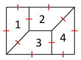
Figure 8: A particular diagram of the non-Mondrian topology at 4-loop with 6 external and 4 internal cuts.

For this diagram, we can first maximally impose all 6 available external cuts, as indicated by the red segments around its rim. Following the convention of external face variables in [3, 4], these 6 cuts result in $x_{1}\!=\!y_{1}\!=\!y_{2}\!=\!z_{4}\!=\!w_{4}\!=\!w_{3}\!=\!0$, which can simplify the six $D$’s as

$$D_{12}=x_{2}(z_{1}-z_{2}),$$ (78)

$$D_{34}=z_{3}(x_{4}-x_{3}),$$

$$D_{13}=x_{3}(z_{1}-z_{3})+y_{3}w_{1},$$

$$D_{24}=z_{2}(x_{4}-x_{2})+y_{4}w_{2},$$

$$D_{23}=(x_{3}-x_{2})(z_{2}-z_{3})+y_{3}w_{2},$$

$$D_{14}=x_{4}z_{1}+y_{4}w_{1}.$$

Now for part of these $D$’s as internal propagators, we can either cut them or impose their positivity. Note that there is no way to further cut $D_{14}$ by fixing one variable, as discussed in [2], but since it is manifestly positive already, there is no positivity condition to be imposed. By tentatively setting

$$z_{1}=z_{2},~{}~{}x_{4}=x_{3},~{}~{}z_{3}=z_{2}+\frac{y_{3}w_{1}}{x_{3}}\equiv\hat{z}_{3},~{}~{}x_{2}=x_{3}+\frac{y_{4}w_{2}}{z_{2}}\equiv\hat{x}_{2},$$ (79)

we can turn off $D_{12},D_{34},D_{13},D_{24}$, and incidentally we have

$$D_{23}=y_{3}w_{2}\left(1+\frac{y_{4}w_{1}}{x_{3}z_{2}}\right),$$ (80)

which is also manifestly positive, therefore we are done with this further simplification. Note the solutions of $D_{12}\!=\!D_{34}\!=\!D_{13}\!=\!D_{24}\!=\!0$, namely (79), are also manifestly positive. In contrast, solutions that involve relative minus signs, such as $z_{3}\!=\!z_{2}\!-\!y_{3}w_{1}/x_{3}$, are clearly not, since we also have to impose $z_{2}\!>\!y_{3}w_{1}/x_{3}$. Such a category of manifestly positive solutions will be named as the positive cuts.

The further 4 internal cuts are also drawn in figure 8, and besides this diagram, other diagrams of all topologies, orientations and configurations of loop numbers at 4-loop that survive these 10 cuts, are given in figure 9, as can be enumerated from the topologies in figure 7 then picked out by identifying all 10 poles $x_{1},y_{1},y_{2},z_{4},w_{4},w_{3},D_{12},D_{34},D_{13},D_{24}$. Let’s define the sum of these 9 surviving diagrams as a function of $x,y,z,w$ (we only sum their proper numerators as usual)

$$S\,(x_{1},y_{1},z_{1},w_{1},x_{2},y_{2},z_{2},w_{2},x_{3},y_{3},z_{3},w_{3},x_{4},y_{4},z_{4},w_{4})$$ (81)

$$= \,x_{2}x_{3}x_{4}z_{1}z_{2}z_{3}\,y_{3}w_{2}\,D_{14}(s_{2}\,y_{4}w_{1}+D_{14})+x_{2}x_{4}z_{1}z_{3}\,y_{3}w_{2}\,D_{14}(x_{4}z_{2}\,y_{3}w_{1}+x_{3}z_{1}\,y_{4}w_{2})$$

$$+x_{2}x_{4}z_{1}z_{3}\,y_{3}y_{4}w_{1}w_{2}\,(y_{3}w_{2}D_{14}+x_{2}z_{3}D_{14}+y_{4}w_{1}D_{23}+x_{4}z_{1}D_{23}+s_{1}D_{14}D_{23}),$$

where $s_{1}$ and $s_{2}$ are coefficients to be determined. Since the cross diagram in figure 9 can survive these 10 cuts like the non-Mondrian one in figure 7, we can fix both $s_{1}$ and $s_{2}$ in only one equation. In contrast, if we impose all 8 external cuts available for the cross diagram, the non-Mondrian one cannot survive these cuts and hence $s_{2}$ will disappear in this equation, then one more equation that involves $s_{2}$ is needed. This explains why to determine $s_{1}$ and $s_{2}$ in one equation, we choose a set of external cuts in the non-Mondrian diagram which has less available external cuts than the cross diagram, as it is a general trick to minimize the number of equations needed for determining all coefficients.

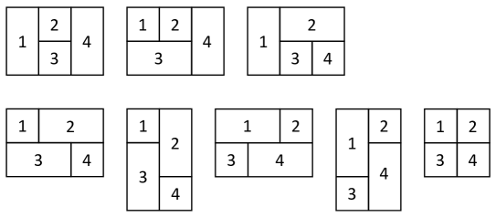
Figure 9: All other 8 diagrams that survive the 10 cuts $x_{1}\!=\!y_{1}\!=\!y_{2}\!=\!z_{4}\!=\!w_{4}\!=\!w_{3}\!=\!D_{12}\!=\!D_{34}\!=\!D_{13}\!=\!D_{24}\!=\!0$.

On the other hand, from the positivity conditions of the amplituhedron we have the following dimensionless ratios with respect to $D_{12},D_{34},D_{13},D_{24}$:

$$\frac{z_{1}}{z_{1}-z_{2}}=\frac{x_{2}z_{1}}{D_{12}}\to\frac{\hat{x}_{2}z_{2}}{D_{12}},$$ (82)

$$\frac{x_{4}}{x_{4}-x_{3}}=\frac{z_{3}x_{4}}{D_{34}}\to\frac{\hat{z}_{3}x_{3}}{D_{34}},$$

$$z_{3}\left(\frac{1}{z_{3}}-\frac{1}{z_{3}-\hat{z}_{3}}\right)=\frac{x_{3}\hat{z}_{3}}{D_{13}},$$

$$x_{2}\left(\frac{1}{x_{2}}-\frac{1}{x_{2}-\hat{x}_{2}}\right)=\frac{z_{2}\hat{x}_{2}}{D_{24}},$$

where $\hat{x}_{2}$ and $\hat{z}_{3}$ are defined in (79), and $\to$ denotes some variables are replaced by the solutions of cuts. Since $D_{14}$ and $D_{23}$ are trivially positive, we get the proper numerator

$$(\hat{x}_{2}x_{3}z_{2}\hat{z}_{3})^{2}D_{14}D_{23}=\left[\left(x_{3}+\frac{y_{4}w_{2}}{z_{2}}\right)\left(z_{2}+\frac{y_{3}w_{1}}{x_{3}}\right)x_{3}z_{2}\right]^{2}y_{3}w_{2}\left(1+\frac{y_{4}w_{1}}{x_{3}z_{2}}\right)(x_{3}z_{2}+y_{4}w_{1}).$$ (83)

Now the critical step is to equate the deformed $S$ defined in (81) on the 10 cuts and the quantity above, or consider their difference

$$\,S\left(0\,,\,0\,,z_{2},w_{1},x_{3}\!+\!\frac{y_{4}w_{2}}{z_{2}},\,0\,,z_{2},w_{2},x_{3},y_{3},z_{2}\!+\!\frac{y_{3}w_{1}}{x_{3}},\,0\,,x_{3},y_{4},\,0\,,\,0\right)$$ (84)

$$-\left[\left(x_{3}+\frac{y_{4}w_{2}}{z_{2}}\right)\left(z_{2}+\frac{y_{3}w_{1}}{x_{3}}\right)x_{3}z_{2}\right]^{2}y_{3}w_{2}\left(1+\frac{y_{4}w_{1}}{x_{3}z_{2}}\right)(x_{3}z_{2}+y_{4}w_{1})$$

$$= \,y_{3}y_{4}w_{1}w_{2}\left(1+\frac{y_{4}w_{1}}{x_{3}z_{2}}\right)(x_{3}z_{2}+y_{3}w_{1})(x_{3}z_{2}+y_{4}w_{2})\left[(1+s_{1})y_{3}w_{2}(x_{3}z_{2}+y_{4}w_{1})+(1+s_{2})x_{3}^{2}z_{2}^{2}\right],$$

then it is clear that to make this difference vanish, we must take $s_{1}\!=\!s_{2}\!=\!-1$, which agrees with [5]. For this 4-loop case, we see the analysis and calculation are very simple, due to there is in fact no positivity condition to be imposed – all $D$’s are either cut or manifestly positive. But in general this simplicity does not always occur, as immediately at 5-loop we will encounter some quite nontrivial and hence much more complicated examples. Still, with the aid of positive cuts, our calculational capability is greatly enhanced so that unlike the hopeless case study of (71), we manage to tackle all 5-loop examples.

3 Positive Cuts at 5-loop

For the 5-loop application of positive cuts, there is nothing new in its principle but we will see much more complexity in various techniques, as well as its miraculous agreement with previous knowledge. As usual, we first enumerate all 34 distinct DCI topologies at 5-loop: figure 10 lists all 24 Mondrian DCI topologies labelled by $T_{1},\ldots,T_{24}$, as indicated by the red subscripts, and figure 11 all 10 non-Mondrian ones labelled by $T_{25},\ldots,T_{34}$ similarly.

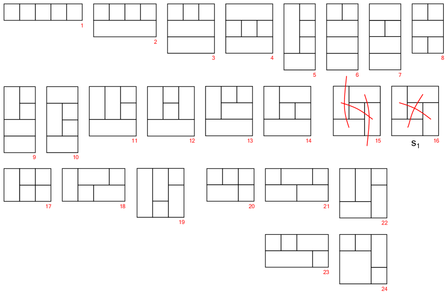
Figure 10: Mondrian DCI topologies $T_{1},\ldots,T_{24}$ at 5-loop. $T_{16}$ assigned with $s_{1}$ is a non-rung-rule topology (it is generated by the substitution rule).

Note that there exist two distinct choices of DCI numerator for the pinwheel’s pole structure, namely $T_{15}$ and $T_{16}$ given in figure 10, so we must explicitly draw their numerators while suppressing those of the rest Mondrian topologies as they can be uniquely inferred from the rung rule. And for non-Mondrian ones in figure 11, we draw all numerators explicitly since the rung rule cannot account for all of them. Among all these 34 topologies, $T_{16},T_{30}$ are generated by applying the substitution rule to the 4-loop counterparts in figure 7, which also preserves coefficients [6], while the rules for $T_{32},T_{33},T_{34}$ are unknown, and the rest are generated by the rung rule. As a simplified demonstration, we focus on non-rung-rule topologies only, so $T_{16},T_{30},T_{32},T_{33},T_{34}$ assigned with coefficients $s_{1},s_{2},s_{3},s_{4},s_{5}$ respectively are of our concern. Let’s now determine these coefficients one by one using the amplituhedron approach.

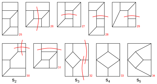
Figure 11: Non-Mondrian DCI topologies $T_{25},\ldots,T_{34}$ at 5-loop. $T_{30},T_{32},T_{33},T_{34}$ assigned with $s_{2},s_{3},s_{4},s_{5}$ respectively are non-rung-rule topologies ($T_{30}$ is generated by the substitution rule while $T_{32},T_{33},T_{34}$ are neither generated by the rung nor substitution rule).

Figure 12: A particular diagram of $T_{16}$ at 5-loop with 8 external cuts.

3.1 Determination of $s_{1}$

To determine $s_{1}$, let’s consider a particular diagram of DCI topology $T_{16}$ given in figure 12. As usual, we can maximally impose all 8 available external cuts, as indicated by the red segments. These 8 cuts result in $x_{1}\!=\!y_{1}\!=\!y_{2}\!=\!z_{2}\!=\!z_{3}\!=\!w_{3}\!=\!w_{4}\!=\!x_{4}\!=\!0$, which can simplify the ten $D$’s as

$$D_{12}=x_{2}z_{1},~{}~{}D_{23}=y_{3}w_{2},~{}~{}D_{34}=x_{3}z_{4},~{}~{}D_{14}=y_{4}w_{1},$$ (85)

$$D_{13}=x_{3}z_{1}+y_{3}w_{1},~{}~{}D_{24}=x_{2}z_{4}+y_{4}w_{2},$$

as well as

$$D_{15}=x_{5}z_{1}+y_{5}w_{1}-x_{5}z_{5}-y_{5}w_{5},$$ (86)

$$D_{25}=z_{5}x_{2}+y_{5}w_{2}-x_{5}z_{5}-y_{5}w_{5},$$

$$D_{35}=z_{5}x_{3}+w_{5}y_{3}-x_{5}z_{5}-y_{5}w_{5},$$

$$D_{45}=x_{5}z_{4}+w_{5}y_{4}-x_{5}z_{5}-y_{5}w_{5}.$$

Since $D_{12},D_{23},D_{34},D_{14},D_{13},D_{24}$ are manifestly positive, we only need to either cut $D_{15},D_{25},D_{35},D_{45}$ or impose their positivity. However, there is no straightforward positive cut for positivity conditions of the form $x\!+\!y\!>\!a$ in this case – the discussion can be rather complicated. Therefore let’s keep their positivity and see what happens next, in fact, $D_{15},D_{25},D_{35},D_{45}$ totally decouple partly due to the symmetry of the 8 external cuts in figure 12, so that we can impose the positivity for each $D_{i5}$ individually. This leads to the simple proper numerator

$$N= \,(x_{5}z_{1}+y_{5}w_{1})(z_{5}x_{2}+y_{5}w_{2})(z_{5}x_{3}+w_{5}y_{3})(x_{5}z_{4}+w_{5}y_{4})D_{12}D_{23}D_{34}D_{14}D_{13}D_{24}$$ (87)

$$= \,(x_{5}z_{1}+y_{5}w_{1})(z_{5}x_{2}+y_{5}w_{2})(z_{5}x_{3}+w_{5}y_{3})(x_{5}z_{4}+w_{5}y_{4})\,x_{2}x_{3}z_{1}z_{4}\,y_{3}y_{4}w_{1}w_{2}\,(x_{3}z_{1}+y_{3}w_{1})(x_{2}z_{4}+y_{4}w_{2}).$$

On the other hand, diagrams of all topologies, orientations and configurations of loop numbers at 5-loop that survive these 8 cuts are summarized below:

$$\begin{array}[]{cccccccccc}~{}T_{8}{}&~{}T_{15}{}&~{}T_{16}{}&~{}T_{20}{}&~{}T_{21}{}&~{}T_{22}{}&~{}T_{23}{}&~{}T_{24}{}&~{}T_{32}{}&~{}T_{33}{}\\ \hline\cr 2&4&1&8&4&8&8&8&4&2\end{array}$$ (88)

where all orientations generated by dihedral symmetry of these topologies contribute and each orientation exactly contributes one configuration of loop numbers, as given by the numbers of contributing diagrams of each $T_{i}$ above. It is easy to enumerate all of them, and the sum of their proper numerators is

$$\,S\,(x_{1},y_{1},z_{1},w_{1},x_{2},y_{2},z_{2},w_{2},x_{3},y_{3},z_{3},w_{3},x_{4},y_{4},z_{4},w_{4},x_{5},y_{5},z_{5},w_{5})$$ (89)

$$= \,x_{2}x_{3}x_{5}z_{1}z_{4}z_{5}\,y_{3}y_{4}y_{5}w_{1}w_{2}w_{5}\,(S_{8}+S_{15-16}+S_{20}+S_{21}+S_{22}+S_{23}+S_{24}+S_{32}+S_{33}),$$

where for compactness we have factored out a common factor, and each piece in the sum is given by

$$S_{8}=\frac{y_{5}w_{5}}{x_{5}z_{5}}D_{13}D_{14}D_{23}D_{24}+\frac{x_{5}z_{5}}{y_{5}w_{5}}D_{12}D_{13}D_{24}D_{34},~{}~{}~{}~{}~{}~{}~{}~{}~{}~{}~{}~{}~{}~{}~{}~{}~{}~{}~{}~{}~{}~{}~{}~{}~{}~{}~{}~{}~{}~{}~{}~{}~{}~{}~{}~{}~{}~{}~{}~{}~{}~{}~{}~{}~{}~{}~{}~{}~{}~{}~{}~{}$$ (90)

$$S_{15-16}=D_{13}D_{24}(x_{3}z_{1}D_{24}+y_{3}w_{1}D_{24}+x_{2}z_{4}D_{13}+y_{4}w_{2}D_{13}+s_{1}D_{13}D_{24}),~{}~{}~{}~{}~{}~{}~{}~{}~{}~{}~{}~{}~{}~{}~{}~{}~{}~{}~{}~{}~{}~{}~{}~{}~{}~{}~{}~{}~{}~{}~{}$$ (91)

$$S_{20}= -\frac{y_{4}}{y_{5}}D_{12}D_{13}D_{24}D_{35}-\frac{y_{3}}{y_{5}}D_{12}D_{13}D_{24}D_{45}-\frac{w_{1}}{w_{5}}D_{13}D_{24}D_{25}D_{34}-\frac{w_{2}}{w_{5}}D_{13}D_{15}D_{24}D_{34}$$ (92)

$$-\frac{z_{4}}{z_{5}}D_{13}D_{15}D_{23}D_{24}-\frac{x_{3}}{x_{5}}D_{13}D_{14}D_{24}D_{25}-\frac{z_{1}}{z_{5}}D_{13}D_{23}D_{24}D_{45}-\frac{x_{2}}{x_{5}}D_{13}D_{14}D_{24}D_{35},~{}~{}~{}\,$$

$$S_{21}=\frac{y_{3}y_{4}w_{5}}{y_{5}}D_{12}D_{13}D_{24}+\frac{y_{5}w_{1}w_{2}}{w_{5}}D_{13}D_{24}D_{34}+\frac{x_{2}x_{3}z_{5}}{x_{5}}D_{13}D_{14}D_{24}+\frac{x_{5}z_{1}z_{4}}{z_{5}}D_{13}D_{23}D_{24},~{}\,$$ (93)

$$S_{22}= \,\frac{x_{3}z_{5}y_{4}}{y_{5}}D_{12}D_{13}D_{24}+\frac{x_{5}z_{4}y_{3}}{y_{5}}D_{12}D_{13}D_{24}+\frac{x_{2}z_{5}w_{1}}{w_{5}}D_{13}D_{24}D_{34}+\frac{x_{5}z_{1}w_{2}}{w_{5}}D_{13}D_{24}D_{34}$$ (94)

$$+ \,\frac{x_{2}y_{3}w_{5}}{x_{5}}D_{13}D_{14}D_{24}+\frac{z_{1}y_{4}w_{5}}{z_{5}}D_{13}D_{23}D_{24}+\frac{x_{3}y_{5}w_{2}}{x_{5}}D_{13}D_{14}D_{24}+\frac{z_{4}y_{5}w_{1}}{z_{5}}D_{13}D_{23}D_{24},$$

$$S_{23}= \,\frac{y_{4}^{2}w_{2}}{y_{5}}D_{12}D_{13}D_{35}+\frac{y_{4}w_{2}^{2}}{w_{5}}D_{13}D_{15}D_{34}+\frac{y_{3}^{2}w_{1}}{y_{5}}D_{12}D_{24}D_{45}+\frac{y_{3}w_{1}^{2}}{w_{5}}D_{24}D_{25}D_{34}$$ (95)

$$+ \,\frac{x_{2}^{2}z_{4}}{x_{5}}D_{13}D_{14}D_{35}+\frac{x_{2}z_{4}^{2}}{z_{5}}D_{13}D_{15}D_{23}+\frac{x_{3}z_{1}^{2}}{z_{5}}D_{23}D_{24}D_{45}+\frac{x_{3}^{2}z_{1}}{x_{5}}D_{14}D_{24}D_{25},~{}~{}~{}~{}~{}~{}~{}~{}~{}~{}~{}~{}\,$$

$$S_{24}= \,\frac{x_{2}z_{4}y_{4}}{y_{5}}D_{12}D_{13}D_{35}+\frac{x_{3}z_{1}y_{3}}{y_{5}}D_{12}D_{24}D_{45}+\frac{x_{3}z_{1}w_{1}}{w_{5}}D_{24}D_{25}D_{34}+\frac{x_{2}z_{4}w_{2}}{w_{5}}D_{13}D_{15}D_{34}$$ (96)

$$+ \,\frac{x_{2}y_{4}w_{2}}{x_{5}}D_{13}D_{14}D_{35}+\frac{z_{1}y_{3}w_{1}}{z_{5}}D_{23}D_{24}D_{45}+\frac{x_{3}y_{3}w_{1}}{x_{5}}D_{14}D_{24}D_{25}+\frac{z_{4}y_{4}w_{2}}{z_{5}}D_{13}D_{15}D_{23},$$

$$S_{32}=s_{3}(y_{3}w_{2}D_{13}D_{14}D_{24}+y_{4}w_{1}D_{13}D_{23}D_{24}+x_{3}z_{4}D_{12}D_{13}D_{24}+x_{2}z_{1}D_{13}D_{24}D_{34}),~{}~{}~{}~{}~{}~{}~{}~{}~{}$$ (97)

$$S_{33}=s_{4}(D_{13}D_{14}D_{23}D_{24}+D_{12}D_{13}D_{24}D_{34}).~{}~{}~{}~{}~{}~{}~{}~{}~{}~{}~{}~{}~{}~{}~{}~{}~{}~{}~{}~{}~{}~{}~{}~{}~{}~{}~{}~{}~{}~{}~{}~{}~{}~{}~{}~{}~{}~{}~{}~{}~{}~{}~{}~{}~{}~{}~{}~{}~{}~{}~{}~{}~{}~{}~{}~{}~{}~{}~{}~{}\,$$ (98)

The difference between the deformed $S$ on the 8 cuts and the proper numerator from positivity conditions is then

$$\,S\,(0\,,\,0\,,z_{1},w_{1},x_{2},\,0\,,\,0\,,w_{2},x_{3},y_{3},\,0\,,\,0\,,\,0\,,y_{4},z_{4},\,0\,,x_{5},y_{5},z_{5},w_{5})$$ (99)

$$-(x_{5}z_{1}+y_{5}w_{1})(z_{5}x_{2}+y_{5}w_{2})(z_{5}x_{3}+w_{5}y_{3})(x_{5}z_{4}+w_{5}y_{4})\,x_{2}x_{3}z_{1}z_{4}\,y_{3}y_{4}w_{1}w_{2}\,(x_{3}z_{1}+y_{3}w_{1})(x_{2}z_{4}+y_{4}w_{2})$$

$$= \,x_{2}x_{3}x_{5}z_{1}z_{4}z_{5}\,y_{3}y_{4}y_{5}w_{1}w_{2}w_{5}\,(x_{3}z_{1}+y_{3}w_{1})(x_{2}z_{4}+y_{4}w_{2})$$

$$\times[(1+s_{1})(x_{3}z_{1}\,y_{4}w_{2}+x_{2}z_{4}\,y_{3}w_{1})+(2+s_{1}+2s_{3}+s_{4})(x_{3}x_{2}z_{1}z_{4}+y_{3}y_{4}w_{1}w_{2})],$$

to make this difference vanish we must take $s_{1}\!=\!-1$ which agrees with [5], and $1\!+\!2s_{3}\!+\!s_{4}\!=\!0$. Even though $s_{3}$ and $s_{4}$ cannot be determined by these 8 external cuts yet, we can determine one with the aid of further cuts then get the other via relation $1\!+\!2s_{3}\!+\!s_{4}\!=\!0$.

3.2 Determination of $s_{2},s_{3},s_{4}$

To figure out $s_{3}$ or $s_{4}$, we have to disentangle $T_{32}$ and $T_{33}$, otherwise combination $(1\!+\!2s_{3}\!+\!s_{4})$ will always obstruct our intention. Since $T_{32}$ has one internal propagator more than $T_{33}$ while their other topological features are identical, it is feasible to impose further internal cuts to kill $T_{33}$ but let $T_{32}$ survive so that $s_{3}$ can be isolated then determined. If we consider a particular diagram of $T_{32}$ given in figure 13, a simplest choice is to impose $D_{12}\!=\!D_{23}\!=\!0$, as one can easily check that none of the diagrams of $T_{33}$ can survive it regardless of orientations and number configurations (we also maintain the 8 external cuts in figure 12).

However, since $D_{12}\!=\!x_{2}z_{1}$ and $D_{23}\!=\!y_{3}w_{2}$, setting $D_{12}\!=\!D_{23}\!=\!0$ will force two external propagators which do not belong to the diagram in figure 12 to vanish. This involves a technical subtlety of composite residues, although there is no problem in this way after some clarification, we prefer to avoid this subtlety for the moment. Therefore, a simplest alternative is to relax one external cut, which is chosen to be $z_{2}$.

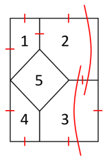
Figure 13: A particular diagram of $T_{32}$ at 5-loop with 7 external and 2 internal cuts. The external cut $z_{2}\!=\!0$ is traded for two internal cuts $D_{12}\!=\!D_{23}\!=\!0$ which are free of the subtlety of composite residues.

In summary, upon the 7 external cuts $x_{1}\!=\!y_{1}\!=\!y_{2}\!=\!z_{3}\!=\!w_{3}\!=\!w_{4}\!=\!x_{4}\!=\!0$, we can further impose

$$z_{1}=z_{2},~{}~{}x_{2}=x_{3}+\frac{y_{3}w_{2}}{z_{2}}\equiv\hat{x}_{2},$$ (100)

so these $7\!+\!2$ cuts can simplify the ten $D$’s as

$$D_{12}=D_{23}=0,~{}~{}D_{34}=x_{3}z_{4},~{}~{}D_{14}=y_{4}w_{1},~{}~{}D_{13}=x_{3}z_{2}+y_{3}w_{1}$$ (101)

which are either zero or manifestly positive, as well as

$$D_{15}=x_{5}z_{2}+y_{5}w_{1}-x_{5}z_{5}-y_{5}w_{5},$$ (102)

$$D_{45}=x_{5}z_{4}+w_{5}y_{4}-x_{5}z_{5}-y_{5}w_{5},$$

$$D_{35}=z_{5}x_{3}+w_{5}y_{3}-x_{5}z_{5}-y_{5}w_{5},$$

$$D_{24}=(x_{3}z_{2}+y_{3}w_{2})\left(\frac{z_{4}}{z_{2}}+\frac{y_{4}}{y_{3}+x_{3}z_{2}/w_{2}}-1\right),$$

$$D_{25}=(z_{5}-z_{2})\left(x_{3}+y_{3}\frac{w_{2}}{z_{2}}-x_{5}\right)+y_{5}(w_{2}-w_{5}),$$

again there is no straightforward positive cut for any of these five positivity conditions, so it is better to keep their positivity. In this case, $D_{15},D_{45},D_{35},D_{24},D_{25}$ do not trivially decouple, as we can see it more clearly after the following reorganization:

$$\frac{z_{2}}{z_{5}+y_{5}w_{5}/x_{5}}+\frac{w_{1}}{w_{5}+x_{5}z_{5}/y_{5}}>1,$$ (103)

$$\frac{x_{3}}{x_{5}+y_{5}w_{5}/z_{5}}+\frac{y_{3}}{y_{5}+x_{5}z_{5}/w_{5}}>1,~{}~{}~{}(z_{5}-z_{2})\left(x_{3}+y_{3}\frac{w_{2}}{z_{2}}-x_{5}\right)+y_{5}(w_{2}-w_{5})>0,$$

$$\frac{z_{4}}{z_{5}+y_{5}w_{5}/x_{5}}+\frac{y_{4}}{y_{5}+x_{5}z_{5}/w_{5}}>1,~{}~{}~{}\frac{z_{4}}{z_{2}}+\frac{y_{4}}{y_{3}+x_{3}z_{2}/w_{2}}>1.$$

In the first line we focus on $z_{2},w_{1}$, in the second $x_{3},y_{3}$ and in the third $z_{4},y_{4}$. For the latter two lines, the discussion of imposing positivity is nontrivial, since we need to choose one condition (or both) as the relations among several variables vary. Explicitly, the second line’s discussion depends on how $z_{2}$ varies in the first line, and the third line’s discussion depends on how $x_{3},y_{3}$ vary in the second line. Its technical details are elaborated in appendix A, and below we just present the resulting $d\log$ form after analyzing all possible situations of variables $z_{2},w_{1},w_{2},y_{3},x_{3},z_{4},y_{4}$:

$$\frac{M}{z_{2}^{3}w_{1}w_{2}y_{3}x_{3}z_{4}y_{4}\,D_{15}D_{35}D_{25}D_{45}D_{24}}\equiv\frac{R}{z_{2}w_{1}w_{2}y_{3}x_{3}z_{4}y_{4}},$$ (104)

where the expression of $M$ is given below, as the result simplified by Mathematica, and $R$ is the desired dimensionless ratio.

$M=w_{1}y_{5}(w_{5}x_{5}y_{3}z_{2}^{2}(w_{5}(y_{4}-y_{5})+x_{5}z_{4})(w_{2}y_{4}z_{2}+w_{2}y_{3}z_{4}+x_{3}z_{2}z_{4})+(w_{2}w_{5}y_{4}z_{2}(w_{2}w_{5}y_{3}^{2}(y_{4}-y_{5})+x_{3}(w_{5}y_{3}y_{4}+w_{2}(-y_{3}+y_{4})y_{5}-w_{5}(y_{3}+y_{4})y_{5})z_{2}-(x_{5}^{2}y_{3}+x_{3}^{2}y_{5})z_{2}^{2})+(w_{2}^{2}w_{5}^{2}y_{3}^{3}y_{4}+w_{2}w_{5}y_{3}(w_{5}x_{3}y_{4}(2y_{3}-y_{5})+w_{2}(x_{5}y_{3}(-y_{3}+y_{4})+x_{3}y_{4}y_{5}))z_{2}+(w_{5}y_{3}(-w_{2}x_{5}(2x_{3}+x_{5})y_{3}+x_{3}(w_{5}x_{3}+w_{2}x_{5})y_{4})+x_{3}(w_{2}w_{5}x_{5}y_{3}+(w_{2}-w_{5})(w_{5}x_{3}+w_{2}x_{5})y_{4})y_{5})z_{2}^{2}-w_{5}x_{3}x_{5}((x_{3}+x_{5})y_{3}-x_{3}y_{5})z_{2}^{3})z_{4}+x_{5}(w_{2}y_{3}+x_{3}z_{2})(w_{2}w_{5}y_{3}^{2}+x_{3}(w_{5}(y_{3}-y_{5})+w_{2}y_{5})z_{2})z_{4}^{2})z_{5}+(w_{2}w_{5}y_{4}z_{2}(w_{2}y_{3}(-x_{5}y_{3}+x_{3}y_{4})+x_{3}(x_{3}y_{4}-x_{5}(y_{3}+y_{4}))z_{2})+x_{3}(w_{2}y_{3}+(x_{3}-x_{5})z_{2})(x_{3}z_{2}(w_{5}y_{4}-x_{5}z_{2})+w_{2}(w_{5}y_{3}y_{4}+x_{5}(-y_{3}+y_{4})z_{2}))z_{4}+x_{3}x_{5}(w_{2}y_{3}+x_{3}z_{2})(w_{2}y_{3}+(x_{3}-x_{5})z_{2})z_{4}^{2})z_{5}^{2})+x_{5}z_{2}^{2}(w_{2}^{2}x_{3}y_{5}(w_{5}y_{4}(-y_{3}+y_{4})z_{2}+w_{5}y_{3}(y_{4}-y_{5})z_{4}+x_{5}z_{4}(y_{4}z_{2}+y_{3}(z_{4}-z_{5})))z_{5}-w_{5}x_{3}y_{3}z_{2}z_{4}(w_{5}(y_{4}-y_{5})+x_{5}(z_{4}-z_{5}))(w_{5}y_{5}+x_{5}(-z_{2}+z_{5}))+w_{2}(-w_{5}^{3}y_{3}(y_{4}-y_{5})y_{5}(y_{4}z_{2}+y_{3}z_{4})+w_{5}^{2}x_{5}y_{3}(y_{4}z_{2}+y_{3}z_{4})(-y_{5}(z_{2}+z_{4}-2z_{5})+y_{4}(z_{2}-z_{5}))+x_{3}^{2}x_{5}y_{5}z_{2}z_{4}(z_{4}-z_{5})z_{5}+w_{5}(x_{5}^{2}y_{3}(y_{4}z_{2}+y_{3}z_{4})(z_{2}-z_{5})(z_{4}-z_{5})-x_{3}^{2}y_{5}z_{2}(y_{4}z_{2}-y_{4}z_{4}+y_{5}z_{4})z_{5})));$

To get the overall dimensionless ratio, we also need

$$\frac{z_{1}}{z_{1}-z_{2}}=\frac{x_{2}z_{1}}{D_{12}}\to\frac{\hat{x}_{2}z_{2}}{D_{12}},$$ (105)

$$x_{2}\left(\frac{1}{x_{2}}-\frac{1}{x_{2}-\hat{x}_{2}}\right)=\frac{z_{2}\hat{x}_{2}}{D_{23}},$$

where $\hat{x}_{2}$ is defined in (100), and since the positivity of $D_{34},D_{14},D_{13}$ is trivial, we finally obtain

$$\frac{\hat{x}_{2}z_{2}}{D_{12}}\,\frac{z_{2}\hat{x}_{2}}{D_{23}}\,\frac{D_{34}D_{14}D_{13}}{D_{34}D_{14}D_{13}}\,R=\frac{(\hat{x}_{2}z_{2})^{2}D_{34}D_{14}D_{13}}{D_{12}D_{23}D_{34}D_{14}D_{13}}\,\frac{1}{D_{15}D_{35}D_{25}D_{45}D_{24}}\,\frac{M}{z_{2}^{2}},$$ (106)

therefore the proper numerator is

$$N=\hat{x}_{2}^{2}\,D_{34}D_{14}D_{13}\,M=\left(x_{3}+\frac{y_{3}w_{2}}{z_{2}}\right)^{2}x_{3}z_{4}\,y_{4}w_{1}\,(x_{3}z_{2}+y_{3}w_{1})\,M.$$ (107)

On the other hand, diagrams of all topologies, orientations and configurations of loop numbers at 5-loop that survive these $7\!+\!2$ cuts are summarized below:

$$\begin{array}[]{ccccccccccccccccccc}T_{3}{}&T_{8}{}&T_{9}{}&T_{11}{}&T_{13}{}&T_{14}{}&T_{15}{}&T_{16}{}&T_{17}{}&T_{18}{}&T_{19}{}&T_{20}{}&T_{21}{}&T_{22}{}&T_{23}{}&T_{24}{}&T_{30}{}&T_{31}{}&T_{32}\\ \hline\cr{}\hfil&{}\hfil&{}\hfil&{}\hfil&{}\hfil&{}\hfil&4&1&{}\hfil&{}\hfil&{}\hfil&4{}&2{}&4{}&4{}&4{}&{}\hfil&{}\hfil&2{}\\ 1{}&1{}&1{}&1{}&1{}&1{}&{}\hfil&{}\hfil&1{}&2{}&2{}&1{}&1{}&2{}&1{}&1{}&1{}&1{}&{}\hfil\end{array}$$ (108)

where the first line denotes a subset of diagrams among (89), and the second line the additional surviving contribution due to relaxing $z_{2}\!=\!0$. Again, each orientation of $T_{i}$ can at most contribute one configuration of loop numbers. The sum of their proper numerators is

$$\,S\,(x_{1},y_{1},z_{1},w_{1},x_{2},y_{2},z_{2},w_{2},x_{3},y_{3},z_{3},w_{3},x_{4},y_{4},z_{4},w_{4},x_{5},y_{5},z_{5},w_{5})$$ (109)

$$= \,x_{2}x_{3}x_{5}z_{1}z_{4}z_{5}\,y_{3}y_{4}y_{5}w_{1}w_{2}w_{5}\,(S_{15-16}+S_{20}+S_{21}+S_{22}+S_{23}+S_{24}+S_{32})$$

$$+S_{3}+S_{8}+S_{9}+S_{11}+S_{13}+S_{14}+S_{17-19}+S_{20-24}+S_{30}+S_{31},$$

where each piece in the sum is given by

$$\!\!\!\!S_{15-16}=D_{13}D_{24}(x_{3}z_{1}D_{24}+y_{3}w_{1}D_{24}+x_{2}z_{4}D_{13}+y_{4}w_{2}D_{13}+s_{1}D_{13}D_{24}),~{}~{}~{}~{}~{}~{}~{}~{}~{}~{}~{}~{}~{}$$ (110)

$$~{}~{}S_{20}=-\,0-0-\frac{w_{1}}{w_{5}}D_{13}D_{24}D_{25}D_{34}-\frac{w_{2}}{w_{5}}D_{13}D_{15}D_{24}D_{34}-0-\frac{x_{3}}{x_{5}}D_{13}D_{14}D_{24}D_{25}-0-\frac{x_{2}}{x_{5}}D_{13}D_{14}D_{24}D_{35},$$ (111)

$$S_{21}=0+\frac{y_{5}w_{1}w_{2}}{w_{5}}D_{13}D_{24}D_{34}+\frac{x_{2}x_{3}z_{5}}{x_{5}}D_{13}D_{14}D_{24}+0,~{}~{}~{}~{}~{}~{}~{}~{}~{}~{}~{}~{}~{}~{}~{}~{}~{}~{}~{}~{}~{}~{}~{}~{}~{}~{}~{}~{}~{}~{}~{}~{}~{}~{}~{}~{}~{}~{}~{}~{}~{}~{}~{}~{}~{}~{}~{}~{}~{}~{}~{}~{}~{}~{}\,$$ (112)

$$~{}~{}S_{22}=0+0+\frac{x_{2}z_{5}w_{1}}{w_{5}}D_{13}D_{24}D_{34}+\frac{x_{5}z_{1}w_{2}}{w_{5}}D_{13}D_{24}D_{34}+\frac{x_{2}y_{3}w_{5}}{x_{5}}D_{13}D_{14}D_{24}+0+\frac{x_{3}y_{5}w_{2}}{x_{5}}D_{13}D_{14}D_{24}+0,$$ (113)

$$S_{23}=0+\frac{y_{4}w_{2}^{2}}{w_{5}}D_{13}D_{15}D_{34}+0+\frac{y_{3}w_{1}^{2}}{w_{5}}D_{24}D_{25}D_{34}+\frac{x_{2}^{2}z_{4}}{x_{5}}D_{13}D_{14}D_{35}+0+0+\frac{x_{3}^{2}z_{1}}{x_{5}}D_{14}D_{24}D_{25},\,$$ (114)

$$~{}~{}S_{24}=0+0+\frac{x_{3}z_{1}w_{1}}{w_{5}}D_{24}D_{25}D_{34}+\frac{x_{2}z_{4}w_{2}}{w_{5}}D_{13}D_{15}D_{34}+\frac{x_{2}y_{4}w_{2}}{x_{5}}D_{13}D_{14}D_{35}+0+\frac{x_{3}y_{3}w_{1}}{x_{5}}D_{14}D_{24}D_{25}+0,$$ (115)

$$S_{32}=s_{3}(y_{3}w_{2}D_{13}D_{14}D_{24}+0+0+x_{2}z_{1}D_{13}D_{24}D_{34})~{}~{}~{}~{}~{}~{}~{}~{}~{}~{}~{}~{}~{}~{}~{}~{}~{}~{}~{}~{}~{}~{}~{}~{}~{}~{}~{}~{}~{}~{}~{}~{}~{}~{}~{}~{}~{}~{}~{}~{}~{}~{}~{}~{}~{}~{}~{}~{}~{}~{}~{}~{}~{}~{}~{}~{}~{}~{}$$ (116)

for the subset among (89) (the zeros denote diagrams killed by $D_{12}\!=\!D_{23}\!=\!0$), as well as

$$S_{3}=x_{2}^{3}x_{3}z_{1}z_{2}z_{4}z_{5}\,y_{4}y_{5}w_{1}w_{5}D_{13}D_{14}D_{34}D_{35},~{}~{}~{}~{}~{}~{}~{}~{}~{}~{}~{}~{}~{}~{}~{}~{}~{}~{}~{}~{}~{}~{}~{}~{}~{}~{}~{}~{}~{}~{}~{}~{}~{}~{}~{}~{}$$ (117)

$$S_{8}=x_{2}^{2}x_{3}x_{5}z_{1}z_{2}^{2}z_{4}\,y_{3}y_{4}w_{1}w_{5}D_{13}D_{15}D_{34}D_{45},~{}~{}~{}~{}~{}~{}~{}~{}~{}~{}~{}~{}~{}~{}~{}~{}~{}~{}~{}~{}~{}~{}~{}~{}~{}~{}~{}~{}~{}~{}~{}~{}~{}~{}~{}\,$$ (118)

$$S_{9}=x_{2}^{2}x_{3}x_{5}z_{1}z_{2}z_{4}z_{5}\,y_{4}y_{5}w_{1}^{2}D_{13}D_{24}D_{34}D_{35},~{}~{}~{}~{}~{}~{}~{}~{}~{}~{}~{}~{}~{}~{}~{}~{}~{}~{}~{}~{}~{}~{}~{}~{}~{}~{}~{}~{}~{}~{}~{}~{}~{}~{}~{}~{}$$ (119)

$$S_{11}=x_{2}x_{3}^{3}z_{1}z_{2}z_{4}z_{5}\,y_{4}y_{5}^{2}w_{1}w_{2}w_{5}D_{13}D_{14}D_{24},~{}~{}~{}~{}~{}~{}~{}~{}~{}~{}~{}~{}~{}~{}~{}~{}~{}~{}~{}~{}~{}~{}~{}~{}~{}~{}~{}~{}~{}~{}~{}~{}~{}~{}~{}~{}~{}~{}$$ (120)

$$S_{13}=x_{2}^{2}x_{3}^{2}z_{1}z_{2}z_{4}z_{5}\,y_{4}^{2}y_{5}w_{1}w_{2}w_{5}D_{13}D_{14}D_{35},~{}~{}~{}~{}~{}~{}~{}~{}~{}~{}~{}~{}~{}~{}~{}~{}~{}~{}~{}~{}~{}~{}~{}~{}~{}~{}~{}~{}~{}~{}~{}~{}~{}~{}~{}~{}~{}~{}$$ (121)

$$S_{14}=x_{2}x_{3}^{2}x_{5}z_{1}z_{2}z_{4}z_{5}\,y_{4}^{2}y_{5}w_{1}w_{2}w_{5}D_{13}^{2}D_{24},~{}~{}~{}~{}~{}~{}~{}~{}~{}~{}~{}~{}~{}~{}~{}~{}~{}~{}~{}~{}~{}~{}~{}~{}~{}~{}~{}~{}~{}~{}~{}~{}~{}~{}~{}~{}~{}~{}~{}~{}$$ (122)

$$S_{17-19}= \,x_{2}x_{3}x_{5}z_{1}z_{2}z_{4}z_{5}\,y_{4}y_{5}w_{1}w_{2}D_{13}D_{34}$$ (123)

$$\times(-\,x_{3}D_{15}D_{24}+x_{3}\,y_{4}w_{2}D_{15}+x_{3}\,y_{5}w_{1}D_{24}+x_{2}D_{15}D_{34}+x_{5}D_{13}D_{24}),$$

$$~{}~{}~{}~{}~{}~{}~{}~{}~{}~{}~{}~{}~{}~{}S_{20-24}= \,x_{2}x_{3}x_{5}z_{1}z_{2}z_{4}\,y_{3}^{2}y_{4}w_{1}w_{2}w_{5}D_{15}D_{45}$$ (124)

$$\times\left(-\,D_{13}D_{24}+y_{4}w_{2}D_{13}+\frac{y_{4}}{y_{3}}\,x_{3}z_{2}D_{13}+x_{2}z_{4}D_{13}+y_{3}w_{1}D_{24}+x_{3}z_{1}D_{24}\right),$$

$$S_{30}=s_{2}\,x_{2}x_{3}x_{5}^{2}z_{1}z_{2}z_{4}z_{5}\,y_{3}y_{4}y_{5}w_{1}^{2}w_{2}D_{13}D_{24}D_{34},~{}~{}~{}~{}~{}~{}~{}~{}~{}~{}~{}~{}~{}~{}~{}~{}~{}~{}~{}~{}~{}~{}~{}~{}~{}~{}~{}~{}~{}~{}~{}~{}\,$$ (125)

$$S_{31}=-\,x_{2}x_{3}^{2}x_{5}z_{1}z_{2}z_{4}z_{5}\,y_{3}y_{4}y_{5}w_{1}w_{2}w_{5}D_{13}D_{14}D_{24}~{}~{}~{}~{}~{}~{}~{}~{}~{}~{}~{}~{}~{}~{}~{}~{}~{}~{}~{}~{}~{}~{}~{}~{}~{}~{}~{}~{}~{}~{}\,$$ (126)

for the additional surviving contribution. The difference between the deformed $S$ on the $7\!+\!2$ cuts and the proper numerator is then

$$\,S\left(0\,,\,0\,,z_{2},w_{1},x_{3}\!+\!\frac{y_{3}w_{2}}{z_{2}},\,0\,,z_{2},w_{2},x_{3},y_{3},\,0\,,\,0\,,\,0\,,y_{4},z_{4},\,0\,,x_{5},y_{5},z_{5},w_{5}\right)$$ (127)

$$-\left(x_{3}+\frac{y_{3}w_{2}}{z_{2}}\right)^{2}x_{3}z_{4}\,y_{4}w_{1}\,(x_{3}z_{2}+y_{3}w_{1})\,M$$

$$= \,x_{3}x_{5}z_{4}z_{5}\,y_{3}y_{4}y_{5}w_{1}w_{2}\,(x_{3}z_{2}+y_{3}w_{1})(x_{3}z_{2}+y_{3}w_{2})\left[(x_{3}z_{2}+y_{3}w_{2})\left(\frac{z_{4}}{z_{2}}-1\right)+\,y_{4}w_{2}\right]$$

$$\times[(1+s_{2})x_{3}x_{5}z_{2}z_{4}\,w_{1}+(1+s_{3})w_{5}(x_{3}z_{4}(x_{3}z_{2}+y_{3}w_{2})+y_{3}y_{4}w_{1}w_{2})],$$

to make this difference vanish we must take $s_{2}\!=\!s_{3}\!=\!-1$, so via $1\!+\!2s_{3}\!+\!s_{4}\!=\!0$ we also obtain $\!s_{4}\!=\!+1$, all of which agree with [5]. We see that determining $s_{2}$ is a byproduct of determining $s_{3}$.

It is worth noticing the complexity of 5-loop topologies which have a purely internal loop: the simple case of $T_{16}$ with 8 symmetric external cuts is clearly rather rare, as merely relaxing one cut results in five positivity conditions that do not trivially decouple. In general, the more external cuts a topology has, the easier its calculation might be. We will see how dramatic this qualitative criterion looks from the case of $T_{34}$, which merely has two external cuts less than $T_{16}$ but becomes extremely complicated, even compared to the case of $T_{32}$ which is already very nontrivial.

3.3 Determination of $s_{5}$

To determine $s_{5}$, the coefficient of $T_{34}$, turns out to be the most difficult case at 5-loop. We again consider a particular diagram given in figure 14, in which all 6 available external cuts are imposed, now let’s again impose internal cuts $D_{12}\!=\!D_{23}\!=\!0$ upon $x_{1}\!=\!y_{1}\!=\!z_{2}\!=\!z_{3}\!=\!w_{4}\!=\!x_{4}\!=\!0$. Even though this diagram has only one external cut less than the one in figure 13, it is very different from the latter. In fact, the structure and complexity of the simplified positivity conditions are very sensitive to the choice of cuts.

Figure 14: A particular diagram of $T_{34}$ at 5-loop with 6 external and 2 internal cuts.

Explicitly, for the two internal cuts we can impose

$$w_{2}=w_{3}=w_{1}+\frac{x_{2}z_{1}}{y_{2}}\equiv\hat{w}_{3},$$ (128)

so the ten $D$’s can be simplified as

$$D_{12}=D_{23}=0,~{}~{}D_{14}=y_{4}w_{1}$$ (129)

which are either zero or manifestly positive, as well as

$$D_{13}=z_{1}\left(x_{3}-x_{2}\frac{y_{3}}{y_{2}}\right)\equiv z_{1}x^{\prime}_{3},$$ (130)

$$D_{15}=x_{5}z_{1}+y_{5}w_{1}-x_{5}z_{5}-y_{5}w_{5},$$

$$D_{45}=x_{5}z_{4}+w_{5}y_{4}-x_{5}z_{5}-y_{5}w_{5},$$

$$D_{24}=(x_{2}z_{1}+y_{2}w_{1})\left(\frac{z_{4}}{z_{1}+w_{1}y_{2}/x_{2}}+\frac{y_{4}}{y_{2}}-1\right),$$

$$D_{34}=(x_{2}z_{1}+y_{2}w_{1})\,\frac{y_{3}}{y_{2}}\left(\frac{x_{3}}{y_{3}}\frac{z_{4}}{z_{1}x_{2}/y_{2}+w_{1}}+\frac{y_{4}}{y_{3}}-1\right),$$

$$D_{25}=(y_{5}-y_{2})\left(w_{1}+z_{1}\frac{x_{2}}{y_{2}}-w_{5}\right)+z_{5}(x_{2}-x_{5}),$$

$$D_{35}=(y_{5}-y_{3})\left(w_{1}+z_{1}\frac{x_{2}}{y_{2}}-w_{5}\right)+z_{5}(x_{3}-x_{5}),$$

where $x^{\prime}_{3}$ is defined to trivialize $D_{13}\!>\!0$, and the rest six conditions can be analyzed more clearly after the following reorganization:

$$w_{1}\!+\!z_{1}\frac{x_{5}}{y_{5}}\!>\!w_{5}\!+\!z_{5}\frac{x_{5}}{y_{5}},~{}~{}(y_{5}\!-\!y_{2})\left(\!w_{1}\!+\!z_{1}\frac{x_{2}}{y_{2}}\!-\!w_{5}\!\right)\!+\!z_{5}(x_{2}\!-\!x_{5})\!>\!0,~{}~{}(y_{5}\!-\!y_{3})\left(\!w_{1}\!+\!z_{1}\frac{x_{2}}{y_{2}}\!-\!w_{5}\!\right)\!+\!z_{5}(x_{3}\!-\!x_{5})\!>\!0,$$ (131)

$$\frac{z_{4}}{z_{5}\!+\!y_{5}w_{5}/x_{5}}\!+\!\frac{y_{4}}{y_{5}\!+\!x_{5}z_{5}/w_{5}}\!>\!1,~{}~{}\frac{z_{4}}{z_{1}\!+\!w_{1}y_{2}/x_{2}}\!+\!\frac{y_{4}}{y_{2}}\!>\!1,~{}~{}\frac{z_{4}}{k(z_{1}\!+\!w_{1}y_{2}/x_{2})}\!+\!\frac{y_{4}}{y_{3}}\!>\!1,$$

where $k\!=\!y_{3}x_{2}/(y_{2}x_{3})\!<\!1$ due to $D_{13}\!>\!0$. In the first line we focus on $w_{1},z_{1}$ and in the second $z_{4},y_{4}$, as the second line’s discussion depends on how $w_{1},z_{1}$ vary in the first line, and its technical details are briefly given in appendix B. Below we just present the resulting $d\log$ form after analyzing all possible situations of variables $y_{2},y_{3},y_{5},x_{5},x^{\prime}_{3},w_{5},z_{1},w_{1},y_{4},z_{4}$:

$$\frac{1}{y_{2}y_{3}y_{5}x_{5}x^{\prime}_{3}w_{5}z_{1}w_{1}y_{4}z_{4}\,D_{15}D_{25}D_{35}D_{45}D_{24}D_{34}}\,\frac{\hat{w}_{3}}{D_{23}}\,\frac{y_{2}(M_{1}y_{2}D_{34})+y_{3}M_{2}}{y_{2}^{4}}$$ (132)

$$\equiv \frac{R}{y_{2}y_{3}y_{5}x_{5}x_{3}w_{5}z_{1}w_{1}y_{4}z_{4}},$$

where the expressions of $M_{1}$ and $M_{2}$ simplified by Mathematica can be referred in appendix B, and $R$ is the desired dimensionless ratio, which is explicitly given by

$$R =\frac{x_{3}}{x^{\prime}_{3}}\,\frac{\hat{w}_{3}}{D_{15}D_{25}D_{35}D_{45}D_{24}D_{34}D_{23}}\,\frac{y_{2}(M_{1}y_{2}D_{34})+y_{3}M_{2}}{y_{2}^{4}}$$ (133)

$$=\frac{x_{3}z_{1}\hat{w}_{3}}{D_{13}D_{15}D_{25}D_{35}D_{45}D_{24}D_{34}D_{23}}\,\frac{y_{2}(M_{1}y_{2}D_{34})+y_{3}M_{2}}{y_{2}^{4}}.$$

To get the overall dimensionless ratio, we also need

$$w_{2}\left(\frac{1}{w_{2}}-\frac{1}{w_{2}-\hat{w}_{3}}\right)=\frac{y_{2}\hat{w}_{3}}{D_{12}},$$ (134)

where $\hat{w}_{3}$ is defined in (128), and since the positivity of $D_{14}$ is trivial, we finally obtain

$$\frac{y_{2}\hat{w}_{3}}{D_{12}}\,\frac{D_{14}}{D_{14}}\,R=\frac{y_{2}\hat{w}_{3}D_{14}}{D_{12}D_{14}}\,\frac{x_{3}z_{1}\hat{w}_{3}}{D_{13}D_{15}D_{25}D_{35}D_{45}D_{24}D_{34}D_{23}}\,\frac{y_{2}(M_{1}y_{2}D_{34})+y_{3}M_{2}}{y_{2}^{4}},$$ (135)

therefore the proper numerator is

$$N=\hat{w}_{3}^{2}\,D_{14}\,x_{3}z_{1}\,\frac{y_{2}(M_{1}y_{2}D_{34})+y_{3}M_{2}}{y_{2}^{3}}=\left(w_{1}+\frac{x_{2}z_{1}}{y_{2}}\right)^{2}y_{4}w_{1}\,x_{3}z_{1}\,\frac{y_{2}(M_{1}y_{2}D_{34})+y_{3}M_{2}}{y_{2}^{3}}.$$ (136)

On the other hand, diagrams of all topologies, orientations and configurations of loop numbers at 5-loop that survive these $6\!+\!2$ cuts are summarized below:

$$\small\!\!\!\!\!\!\!\!\!\!\!\!\!\!\!\!\begin{array}[]{cccccccccccccccccccccccccc}T_{1}\!\!&T_{3}\!&T_{5}&T_{6}\!&T_{7}\!&T_{8}&T_{9}\!\!&T_{10}\!&T_{11}\!&T_{13}\!&T_{14}\!&T_{15}\!&T_{16}\!&T_{17}\!\!&T_{18}&T_{19}&T_{20}&T_{21}&T_{22}&T_{23}&T_{24}\!&T_{25}\!&T_{30}\!&T_{31}\!&T_{32}\!&T_{34}\\ \hline\cr{}\hfil&{}\hfil&{}\hfil&{}\hfil&{}\hfil&{}\hfil&{}\hfil&{}\hfil&{}\hfil&{}\hfil&{}\hfil&4\!&1\!&{}\hfil&{}\hfil&{}\hfil&4&2&4&4&4\!&{}\hfil&{}\hfil&{}\hfil&2\!&{}\hfil\\ 1\!\!&2\!&(4)\!+\!1&(3)\!+\!1\!&2\!&(3)&(4)\!+\!3\!\!&1\!&1\!&2\!&2\!&{}\hfil&{}\hfil&2\!\!&(2)\!+\!3&(2)\!+\!3&(3)\!+\!1&(3)&(3)\!+\!3&(4)\!+\!4&(4)\!+\!4\!&2\!&2\!&1\!&{}\hfil&1\end{array}$$ (137)

where the first line denotes a subset of diagrams among (89) which are identical to those given in (109), and the second line the additional surviving contribution. Now for some $T_{i}$’s, a particular orientation can contribute more than one configuration of loop numbers, as the numbers in parentheses above denote this kind of multiplicity. An explicit example is $(4)\!+\!1$ for $T_{5}$ corresponding to the diagrams given in figure 15, of which the first four with different number configurations share the same orientation.

Figure 15: The $(4)\!+\!1$ multiplicity of $T_{5}$.

The sum of their proper numerators is

$$\,S\,(x_{1},y_{1},z_{1},w_{1},x_{2},y_{2},z_{2},w_{2},x_{3},y_{3},z_{3},w_{3},x_{4},y_{4},z_{4},w_{4},x_{5},y_{5},z_{5},w_{5})$$ (138)

$$= \,x_{2}x_{3}x_{5}z_{1}z_{4}z_{5}\,y_{3}y_{4}y_{5}w_{1}w_{2}w_{5}\,(S_{15-16}\!+\!S_{20}\!+\!S_{21}\!+\!S_{22}\!+\!S_{23}\!+\!S_{24}\!+\!S_{32}\!+\!S_{34})$$

$$+\!S_{1}\!+\!S_{3}\!+\!S_{5}\!+\!S_{6}\!+\!S_{7}\!+\!S_{8}\!+\!S_{9}\!+\!S_{10}\!+\!S_{11}\!+\!S_{13}\!+\!S_{14}\!+\!S_{17-19}\!+\!S^{\prime}_{20-24}\!+\!S_{25}\!+\!S_{30}\!+\!S_{31}.$$

Recall that $S_{15-16},S_{20},S_{21},S_{22},S_{23},S_{24},S_{32}$ are already given in (109), while

$$S_{34}=s_{5}\,y_{2}w_{3}D_{13}D_{14}D_{24}$$ (139)

is the extra term in the second line above, and each piece in the third line is given by

$$S_{1}=y_{2}y_{3}y_{4}y_{5}w_{1}w_{2}w_{3}w_{5}D_{13}D_{14}D_{15}D_{24}D_{25}D_{34},~{}~{}~{}~{}~{}~{}~{}~{}~{}~{}~{}~{}~{}~{}~{}~{}~{}~{}~{}~{}~{}~{}~{}~{}~{}~{}~{}~{}~{}~{}~{}~{}~{}~{}~{}~{}~{}~{}~{}~{}~{}~{}~{}~{}~{}~{}~{}~{}~{}~{}~{}~{}~{}~{}~{}~{}~{}~{}~{}~{}$$ (140)

$$S_{3}=x_{3}x_{5}z_{4}z_{5}\,y_{2}y_{3}y_{4}y_{5}w_{1}w_{2}^{3}D_{13}D_{14}D_{15}D_{34}+x_{3}x_{5}z_{1}z_{5}\,y_{2}^{3}y_{4}w_{1}w_{2}w_{3}w_{5}D_{13}D_{14}D_{34}D_{45},~{}~{}~{}~{}~{}~{}~{}~{}~{}~{}$$ (141)

$$S_{5}= \,x_{2}x_{3}x_{5}z_{1}^{3}\,y_{4}^{2}w_{1}w_{2}w_{3}w_{5}(y_{3}y_{5}D_{24}D_{25}D_{34}+y_{2}y_{5}D_{24}D_{34}D_{35}+y_{2}y_{3}D_{24}D_{35}D_{45}+y_{2}y_{3}D_{25}D_{34}D_{45})$$ (142)

$$+x_{2}x_{3}x_{5}z_{4}^{3}\,y_{2}y_{3}y_{4}y_{5}w_{1}^{2}w_{2}w_{3}D_{13}D_{15}D_{25},$$

$$\!\!\!\!\!\!\!\!\!S_{6}= \,z_{1}\,y_{4}w_{1}w_{2}w_{3}w_{5}D_{14}D_{24}\!\left(x_{2}\,y_{3}^{2}y_{5}D_{15}D_{25}D_{34}+x_{3}\,y_{2}^{2}y_{5}D_{15}D_{34}D_{35}+x_{5}\,y_{2}^{2}y_{3}D_{13}D_{35}D_{45}\right)$$ (143)

$$+x_{5}z_{4}\,y_{2}y_{3}y_{4}y_{5}w_{1}w_{2}w_{3}^{2}D_{13}D_{14}D_{15}D_{24}D_{25},$$

$$S_{7}=z_{5}\,y_{2}y_{3}y_{4}y_{5}w_{1}w_{2}w_{3}w_{5}D_{13}D_{14}D_{24}(x_{2}D_{13}D_{45}+x_{3}D_{15}D_{24}),~{}~{}~{}~{}~{}~{}~{}~{}~{}~{}~{}~{}~{}~{}~{}~{}~{}~{}~{}~{}~{}~{}~{}~{}~{}~{}~{}~{}~{}~{}~{}~{}~{}~{}~{}~{}~{}~{}~{}~{}$$ (144)

$$\!\!\!\!\!\!\!\!\!\!\!\!S_{8}=x_{5}z_{1}z_{4}\,y_{4}w_{1}w_{2}D_{14}\!\left(x_{3}\,y_{2}^{2}y_{3}w_{2}w_{5}D_{13}D_{35}D_{45}+x_{2}\,y_{3}^{2}y_{5}w_{3}^{2}D_{15}D_{24}D_{25}+x_{3}\,y_{2}^{2}y_{5}w_{2}w_{3}D_{15}D_{34}D_{35}\right),$$ (145)

$$\!\!\!\!\!\!\!\!\!\!\!\!\!S_{9}= z_{1}^{2}\,y_{4}w_{1}w_{2}w_{3}w_{5}D_{14}\!\left(x_{2}x_{3}\,y_{3}y_{5}^{2}D_{24}D_{25}D_{34}\!+\!x_{2}x_{3}\,y_{2}y_{5}^{2}D_{24}D_{34}D_{35}\!+\!x_{2}x_{5}\,y_{2}y_{3}^{2}D_{24}D_{35}D_{45}\!+\!x_{3}x_{5}\,y_{2}^{2}y_{3}D_{25}D_{34}D_{45}\right)$$ (146)

$$\!+\!x_{2}^{2}z_{1}z_{5}\,y_{3}^{2}y_{4}y_{5}w_{1}w_{2}w_{3}w_{5}D_{13}D_{14}D_{24}D_{45}\!+\!x_{3}z_{4}\,y_{2}y_{3}y_{4}y_{5}w_{1}w_{2}^{2}D_{13}D_{14}D_{15}(x_{3}z_{5}\,w_{5}D_{24}\!+\!x_{5}z_{4}\,w_{3}D_{25}),$$

$$S_{10}=x_{2}x_{3}z_{5}^{2}\,y_{2}y_{3}y_{4}y_{5}w_{1}w_{2}w_{3}w_{5}D_{13}D_{14}^{2}D_{24},~{}~{}~{}~{}~{}~{}~{}~{}~{}~{}~{}~{}~{}~{}~{}~{}~{}~{}~{}~{}~{}~{}~{}~{}~{}~{}~{}~{}~{}~{}~{}~{}~{}~{}~{}~{}~{}~{}~{}~{}~{}~{}~{}~{}~{}~{}~{}~{}~{}~{}~{}~{}~{}~{}~{}~{}~{}~{}~{}~{}~{}~{}~{}~{}~{}~{}\,$$ (147)

$$S_{11}=x_{2}x_{3}x_{5}z_{4}z_{5}^{2}\,y_{2}y_{3}y_{4}y_{5}w_{1}^{3}w_{2}D_{13}D_{24}D_{34},~{}~{}~{}~{}~{}~{}~{}~{}~{}~{}~{}~{}~{}~{}~{}~{}~{}~{}~{}~{}~{}~{}~{}~{}~{}~{}~{}~{}~{}~{}~{}~{}~{}~{}~{}~{}~{}~{}~{}~{}~{}~{}~{}~{}~{}~{}~{}~{}~{}~{}~{}~{}~{}~{}~{}~{}~{}~{}~{}~{}~{}~{}~{}~{}~{}~{}~{}\,$$ (148)

$$S_{13}=x_{2}x_{3}x_{5}z_{4}^{2}z_{5}\,y_{2}y_{3}y_{4}y_{5}w_{1}^{2}w_{2}^{2}D_{13}D_{15}D_{34}+x_{2}x_{3}x_{5}z_{1}^{2}z_{5}\,y_{2}^{2}y_{4}^{2}w_{1}w_{2}w_{3}w_{5}D_{13}D_{34}D_{45},~{}~{}~{}~{}~{}~{}~{}~{}~{}~{}~{}~{}~{}~{}\,$$ (149)

$$S_{14}=x_{2}x_{3}x_{5}z_{5}\,y_{3}y_{4}y_{5}w_{1}w_{2}w_{5}D_{13}D_{24}\!\left(z_{1}^{2}\,y_{4}w_{3}D_{24}+z_{4}^{2}\,y_{2}w_{1}D_{13}\right),~{}~{}~{}~{}~{}~{}~{}~{}~{}~{}~{}~{}~{}~{}~{}~{}~{}~{}~{}~{}~{}~{}~{}~{}~{}~{}~{}~{}~{}~{}~{}~{}~{}~{}~{}~{}~{}~{}~{}$$ (150)

$$\!\!\!\!S_{17-19}= \,x_{2}x_{3}z_{4}z_{5}\,y_{2}y_{3}y_{4}y_{5}w_{1}w_{2}w_{5}D_{13}D_{14}(-\,w_{1}D_{24}D_{35}+w_{1}x_{2}z_{4}D_{35}+w_{1}x_{3}z_{5}D_{24}+w_{2}D_{14}D_{35}+w_{5}D_{13}D_{24})$$ (151)

$$+x_{2}x_{3}z_{1}z_{5}\,y_{3}y_{4}y_{5}w_{1}w_{2}w_{3}w_{5}D_{14}D_{24}(-\,y_{4}D_{13}D_{25}+x_{3}z_{1}y_{4}D_{25}+x_{2}z_{5}\,y_{4}D_{13}+y_{3}D_{14}D_{25}+y_{5}D_{13}D_{24})$$

$$+x_{2}x_{3}z_{1}z_{5}\,y_{2}y_{4}y_{5}w_{1}w_{2}w_{3}w_{5}D_{14}D_{34}D_{35}(x_{2}z_{1}\,y_{4}+y_{2}D_{14}),$$

$$\!\!\!\!\!S^{\prime}_{20-24}= \left(x_{2}x_{3}x_{5}z_{1}z_{4}z_{5}\,y_{2}y_{4}y_{5}w_{1}^{2}w_{3}D_{24}D_{34}D_{35}\!+\!x_{2}^{2}x_{3}z_{1}z_{4}z_{5}\,y_{2}y_{4}y_{5}w_{1}w_{3}w_{5}D_{14}D_{34}D_{35}\right.$$ (152)

$$\left.\!\!\!+x_{2}x_{3}x_{5}z_{1}z_{4}z_{5}\,y_{2}^{2}y_{4}w_{1}w_{3}w_{5}D_{13}D_{34}D_{45}\right)(x_{2}z_{1}\!+\!y_{2}w_{1})$$

$$\!\!\!+\!x_{2}x_{3}x_{5}z_{1}^{2}z_{4}\,y_{2}y_{3}y_{4}w_{1}w_{2}w_{5}D_{35}D_{45}\left(\!-D_{13}D_{24}\!+\!x_{2}z_{4}D_{13}\!+\!y_{4}w_{2}D_{13}\!+\!\frac{z_{4}}{z_{1}}\,y_{2}w_{1}D_{13}\!+\!x_{3}z_{1}D_{24}\!+\!y_{3}w_{1}D_{24}\!\right)$$

$$\!\!\!+\!x_{2}x_{3}x_{5}z_{1}^{2}z_{4}\,y_{2}y_{3}y_{4}w_{1}w_{3}w_{5}D_{25}D_{34}D_{45}(x_{2}z_{1}\!+\!y_{2}w_{1})$$

$$\!\!\!\!\!\!\!\!\!\!\!\!\!\!\!\!\!\!\!\!\!\!\!\!\!\!\!\!\!\!\!\!\!\!+\!x_{2}x_{3}x_{5}z_{1}^{2}z_{4}\,y_{3}y_{4}y_{5}w_{1}w_{2}w_{3}D_{24}D_{25}\left(\!-D_{15}D_{34}\!-\!\frac{z_{4}}{z_{1}}D_{13}D_{15}\!+\!x_{3}z_{4}D_{15}\!+\!y_{4}w_{3}D_{15}\!+\!\frac{z_{4}}{z_{1}}\,y_{3}w_{1}D_{15}\!+\!x_{5}z_{1}D_{34}\!+\!y_{5}w_{1}D_{34}\!\right)$$

$$\!\!\!+\!x_{2}x_{3}x_{5}z_{1}z_{4}^{2}\,y_{3}y_{4}y_{5}w_{1}w_{2}w_{3}D_{13}D_{15}D_{25}(x_{2}z_{4}\!+\!y_{4}w_{2})$$

$$\!\!\!+\!x_{2}x_{3}x_{5}z_{1}^{2}z_{4}\,y_{2}y_{4}y_{5}w_{1}w_{2}w_{3}D_{34}D_{35}\left(\!-D_{15}D_{24}\!+\!x_{2}z_{4}D_{15}\!+\!y_{4}w_{2}D_{15}\!+\!\frac{z_{4}}{z_{1}}\,y_{2}w_{1}D_{15}\!+\!x_{5}z_{1}D_{24}\!+\!y_{5}w_{1}D_{24}\!\right),$$

$$S_{25}=-\,x_{2}x_{3}z_{5}\,y_{2}y_{3}y_{4}y_{5}w_{1}w_{2}w_{3}w_{5}D_{13}D_{14}D_{24}(z_{4}D_{15}+z_{1}D_{45}),~{}~{}~{}~{}~{}~{}~{}~{}~{}~{}~{}~{}~{}~{}~{}~{}~{}~{}~{}~{}~{}~{}~{}~{}~{}~{}~{}~{}~{}~{}~{}~{}~{}~{}~{}~{}~{}~{}~{}~{}~{}~{}\,$$ (153)

$$S_{30}=s_{2}\,x_{2}x_{3}z_{1}z_{4}z_{5}\,y_{3}y_{4}y_{5}w_{1}w_{2}w_{5}D_{13}D_{14}D_{24}(x_{2}\,y_{5}w_{3}+x_{3}\,y_{2}w_{5}),~{}~{}~{}~{}~{}~{}~{}~{}~{}~{}~{}~{}~{}~{}~{}~{}~{}~{}~{}~{}~{}~{}~{}~{}~{}~{}~{}~{}~{}~{}~{}~{}~{}~{}~{}~{}~{}~{}~{}$$ (154)

$$S_{31}=-\,x_{2}x_{3}x_{5}z_{1}z_{4}z_{5}\,y_{2}y_{3}y_{4}y_{5}w_{1}^{2}w_{2}w_{5}D_{13}D_{24}D_{34}.~{}~{}~{}~{}~{}~{}~{}~{}~{}~{}~{}~{}~{}~{}~{}~{}~{}~{}~{}~{}~{}~{}~{}~{}~{}~{}~{}~{}~{}~{}~{}~{}~{}~{}~{}~{}~{}~{}~{}~{}~{}~{}~{}~{}~{}~{}~{}~{}~{}~{}~{}~{}~{}~{}~{}~{}~{}~{}~{}\,$$ (155)

The difference between the deformed $S$ on the $6\!+\!2$ cuts and the proper numerator is then

$$\,S\left(0\,,\,0\,,z_{1},w_{1},x_{2},y_{2},\,0\,,w_{1}\!+\!\frac{x_{2}z_{1}}{y_{2}},x_{3},y_{3},\,0\,,w_{1}\!+\!\frac{x_{2}z_{1}}{y_{2}},\,0\,,y_{4},z_{4},\,0\,,x_{5},y_{5},z_{5},w_{5}\right)$$ (156)

$$-\left(w_{1}+\frac{x_{2}z_{1}}{y_{2}}\right)^{2}y_{4}w_{1}\,x_{3}z_{1}\,\frac{y_{2}(M_{1}y_{2}D_{34})+y_{3}M_{2}}{y_{2}^{3}}$$

$$= \,x_{2}x_{3}x_{5}z_{1}^{2}z_{4}z_{5}\,y_{3}y_{4}^{2}y_{5}w_{1}^{2}w_{5}\,(x_{3}y_{2}-x_{2}y_{3})\left(w_{1}+\frac{x_{2}z_{1}}{y_{2}}\right)^{2}\left[x_{2}z_{4}+(y_{4}-y_{2})\left(w_{1}+\frac{x_{2}z_{1}}{y_{2}}\right)\right](s_{5}-1),$$

to make this difference vanish we must take $s_{5}\!=\!+1$, which agrees with [6].

This completes the determination of $s_{1},s_{2},s_{3},s_{4},s_{5}$ for all five non-rung-rule topologies at 5-loop.

4 Beyond 5-loop Order?

It is clear that for the 4- and 5-loop 4-particle amplituhedra we are no longer using the Mondrian diagrammatics, instead we use the purely amplituhedronic way to obtain the $d\log$ forms from positivity conditions simplified by external and internal cuts, which are similar to the traditional unitarity cuts. As discussed in the end of [4], it is appealing to generalize the Mondrian diagrammatics to include the non-Mondrian complexity. In [7] there is some kind of evidence about how the Mondrian DCI topologies can be related to non-Mondrian ones, and it would be interesting to prove those rules which determine the coefficients of non-rung-rule topologies from the amplituhedronic perspective. All the effort on discovering new rules and patterns finally aims to help us go beyond the current understanding of the 5-loop case, such as to explain the coefficient $+2$ of a special 6-loop DCI topology in [8] since we believe a simple integer coefficient must have a simple origin. The brute-force calculation merely using positivity conditions might be significantly simplified by clever new observations, as we have witnessed in the Mondrian diagrammatics at 3-loop and the positive cuts at 4- and 5-loop. After extracting sufficient deeper features of positivity conditions, it is even possible to conceive a purely combinatoric description of the amplituhedron.

Still, the standard geometric way has a lot to be excavated beyond the current primitive level. When we use positive cuts to determine the coefficient of a particular DCI topology, this looks like “projecting” the entire amplituhedron onto a subspace that contains a subset of all boundaries, we then would like to get more intuition of its geometric interpretation. And why the DCI topologies must be planar, as a basis in what sense they are complete, how this completeness is related to the triangulation of amplituhedron, as well as what role dual conformal invariance plays in the geometric picture, are very vague so far while we believe clarification of these questions will be a significant progress. When searching for various novel formalisms and connections to mathematics to better aid the practical calculation of physical integrands at sufficiently higher loop orders, we will also pay attention to some aspects discussed in [9, 10, 11] which may provide unexpected inspirations. For example, it is interesting to explore how the off-shell finiteness finds its basis in the amplituhedronic setting. And starting at 8-loop [12, 13], novelties such as fractional coefficients and non-$d\log$ contributions also call for amplituhedronic explanations, if the amplituhedron manages to pass all the lower loop tests.

Besides the outlook, it is also helpful to give some remarks on the technical aspects. To simplify the determination of coefficients as much as possible, we must maximally utilize the crucial difference in pole structure of DCI topologies, namely, we will impose sufficient cuts to isolate the particular diagram under consideration while minimizing its accompanying surviving diagrams of different topologies. Note that in our convention, diagrams with the same denominator but different numerators such that they cannot be related to each other by dihedral symmetry, are considered as different DCI topologies, such as $T_{15}$ and $T_{16}$ in figure 10. If finally it is inevitable to deal with these accompanying diagrams, we can still use cuts to separate them, so that their coefficients must satisfy independent sub-equalities in the overall equality required by positivity conditions.

Also, as we have seen from various examples, the calculation of 4-particle loop integrands from positivity conditions with or without cuts, is magically effective: as long as the final answer is free of spurious poles, it is correct and physical. Besides the possible geometric interpretation using DCI topologies, this mystery should have a more self-contained mathematical reason, which can in return refine the laborious and foamy cancelation of spurious poles. And the process of combining the so-called $d\log$ forms, in fact, indicates properties more general than logarithmic singularities or differential forms, as it only depends on the universal fact that the integrand is a rational function in which physical propagators appear as simple poles. The conjectured positivity conditions further serve as some kind of “residue theorems” to provide an effective prescription for constructing the integrand. Such observations may imply that the $d\log$ forms function beyond their definitions, which may hopefully unleash the possibility to account for the non-$d\log$ novelty from the amplituhedronic perspective at 8-loop and higher.

Finally, it has been appealing to extend the techniques for 4-particle amplituhedron to handle more external particles and various configurations of helicities. Attempts include the recent development using sign flips [14, 15], and the discovery of the key role of 4-particle loop integrand from which the integrand of more particles can be extracted [16]. It is worth noticing that, positivity of the pure loop sector and that of the supersymmetric sector encoding helicities use quite different mathematical prescriptions. This difference somehow obstructs an effective unified framework, while from the perspective of positivity, the 4-particle amplituhedron with pure loop sector only (and the 4-particle sign-flip constraints are trivial) is the simplest object, in particular, it is even simpler than the pure tree amplituhedron.

Appendix A Details of the $d\log$ Form for Determining $s_{2},s_{3},s_{4}$

Below we derive the $d\log$ form for determining $s_{2},s_{3},s_{4}$, with respect to positivity conditions

$$\frac{z_{2}}{z_{5}+y_{5}w_{5}/x_{5}}+\frac{w_{1}}{w_{5}+x_{5}z_{5}/y_{5}}>1,$$ (157)

$$\frac{x_{3}}{x_{5}+y_{5}w_{5}/z_{5}}+\frac{y_{3}}{y_{5}+x_{5}z_{5}/w_{5}}>1,~{}~{}~{}(z_{5}-z_{2})\left(x_{3}+y_{3}\frac{w_{2}}{z_{2}}-x_{5}\right)+y_{5}(w_{2}-w_{5})>0,$$

$$\frac{z_{4}}{z_{5}+y_{5}w_{5}/x_{5}}+\frac{y_{4}}{y_{5}+x_{5}z_{5}/w_{5}}>1,~{}~{}~{}\frac{z_{4}}{z_{2}}+\frac{y_{4}}{y_{3}+x_{3}z_{2}/w_{2}}>1.$$

For later convenience, we define quantities

$$n_{3}=x_{3}+y_{3}\frac{w_{5}}{z_{5}}-x_{5}-\frac{y_{5}w_{5}}{z_{5}},~{}~{}n_{5}=x_{3}+y_{3}\frac{w_{2}}{z_{2}}-x_{5}-y_{5}\,\frac{w_{5}-w_{2}}{z_{5}-z_{2}},$$ (158)

$$p_{3}=y_{5}+\frac{x_{5}z_{5}}{w_{5}},~{}~{}p_{5}=\frac{z_{2}}{w_{2}}\left(x_{5}+y_{5}\,\frac{w_{5}-w_{2}}{z_{5}-z_{2}}\right),~{}~{}p_{35}=y_{5}\,\frac{z_{2}}{z_{2}-z_{5}},$$

$$n_{24}=x_{3}-\frac{w_{2}}{z_{2}}\left(y_{5}+\frac{x_{5}z_{5}}{w_{5}}-y_{3}\right)$$

for the discussion involving $y_{3},x_{3}$, as well as

$$a_{2}=z_{5}+\frac{y_{5}w_{5}}{x_{5}},~{}~{}b_{2}=y_{5}+\frac{x_{5}z_{5}}{w_{5}},~{}~{}a_{4}=z_{2},~{}~{}b_{4}=y_{3}+\frac{x_{3}z_{2}}{w_{2}},~{}~{}z_{4}^{\ast}=\frac{b_{4}-b_{2}}{b_{4}/a_{4}-b_{2}/a_{2}},$$ (159)

$$n_{2}=z_{4}\frac{b_{2}}{a_{2}}+y_{4}-b_{2},~{}~{}n_{4}=z_{4}\frac{b_{4}}{a_{4}}+y_{4}-b_{4},$$

$$A=\left(\frac{1}{z_{4}}-\frac{1}{z_{4}-z_{4}^{\ast}}\right)\frac{1}{n_{4}}+\left(\frac{1}{z_{4}-z_{4}^{\ast}}-\frac{1}{z_{4}-a_{2}}\right)\frac{1}{n_{2}}+\frac{1}{z_{4}-a_{2}}\frac{1}{y_{4}},~{}~{}~{}B=\frac{1}{z_{4}y_{4}}\frac{n_{2}+b_{2}}{n_{2}},$$

$$F=\frac{1}{z_{4}y_{4}}\frac{n_{4}+b_{4}}{n_{4}},~{}~{}~{}G=\left(\frac{1}{z_{4}}-\frac{1}{z_{4}-z_{4}^{\ast}}\right)\frac{1}{n_{2}}+\left(\frac{1}{z_{4}-z_{4}^{\ast}}-\frac{1}{z_{4}-a_{4}}\right)\frac{1}{n_{4}}+\frac{1}{z_{4}-a_{4}}\frac{1}{y_{4}}$$

for the discussion involving $z_{4},y_{4}$. We will also use identities

$$\frac{w_{5}}{z_{5}}-\frac{w_{5}-w_{2}}{z_{5}-z_{2}}=\frac{z_{2}}{z_{2}-z_{5}}\left(\frac{w_{5}}{z_{5}}-\frac{w_{2}}{z_{2}}\right),$$ (160)

$$p_{3}-p_{5}=\frac{z_{2}z_{5}}{w_{2}w_{5}}\frac{x_{5}}{z_{2}-z_{5}}\left(\frac{w_{5}}{z_{5}}-\frac{w_{2}}{z_{2}}\right)\left(z_{5}+\frac{y_{5}w_{5}}{x_{5}}-z_{2}\right).$$

Now let’s analyze all possible situations of variables $z_{2},w_{1},w_{2},y_{3},x_{3},z_{4},y_{4}$, by first separating situations $z_{2}\!<\!z_{5}$, $z_{5}\!<\!z_{2}\!<\!z_{5}\!+\!y_{5}w_{5}/w_{5}$ and $z_{2}\!>\!z_{5}\!+\!y_{5}w_{5}/w_{5}$.

A.1 $z_{2}\!<\!z_{5}$

For $z_{2}\!<\!z_{5}$, the 1st line of (157) in terms of $w_{1}$ is nontrivial. The 2nd condition in its 2nd line becomes

$$x_{3}+y_{3}\frac{w_{2}}{z_{2}}>x_{5}+y_{5}\,\frac{w_{5}-w_{2}}{z_{5}-z_{2}},$$ (161)

and for comparison we can rewrite the 1st condition in the same line as

$$x_{3}+y_{3}\frac{w_{5}}{z_{5}}>x_{5}+y_{5}\frac{w_{5}}{z_{5}},$$ (162)

using the 1st identity in (160), for $w_{2}\!<\!w_{5}z_{2}/z_{5}$ we find

$$w_{2}<w_{5}\frac{z_{2}}{z_{5}}\Longrightarrow\frac{w_{5}}{z_{5}}<\frac{w_{5}-w_{2}}{z_{5}-z_{2}}.$$ (163)

For these two conditions in the 2nd line of (157), in terms of $n_{3}$ and $n_{5}$ defined in (158), we have a clear picture in the $y_{3}$-$x_{3}$ plane: the $x_{3}$-intercept of $n_{3}\!=\!0$ is less than that of $n_{5}\!=\!0$, while its slope is greater than that of $n_{5}\!=\!0$, therefore $n_{5}\!>\!0$ already implies $n_{3}\!>\!0$ in the 1st quadrant.

For the two conditions in the 3rd line of (157), in terms of $n_{2}$ and $n_{4}$ defined in (159), since $z_{2}\!<\!z_{5}\!<\!z_{5}\!+\!y_{5}w_{5}/w_{5}$ and

$$y_{3}+x_{3}\frac{z_{2}}{w_{2}}>y_{3}+x_{3}\frac{z_{5}}{w_{5}}>y_{5}+x_{5}\frac{z_{5}}{w_{5}},$$ (164)

in the $z_{4}$-$y_{4}$ plane the $y_{4}$-intercept of $n_{4}\!=\!0$ is greater than that of $n_{2}\!=\!0$ while its $z_{4}$-intercept is less than that of $n_{2}\!=\!0$, so they intercept at $z_{4}\!=\!z_{4}^{\ast}$ in the 1st quadrant. Its $d\log$ form is given by $A$, where $z_{4}^{\ast}$ and $A$ are defined in (159), and the corresponding geometric picture is given in figure 16.

Figure 16: Geometric picture of the $d\log$ form $A$.

Now for $w_{2}\!>\!w_{5}z_{2}/z_{5}$, similarly we have

$$w_{2}>w_{5}\frac{z_{2}}{z_{5}}\Longrightarrow\frac{w_{5}}{z_{5}}>\frac{w_{5}-w_{2}}{z_{5}-z_{2}},$$ (165)

therefore $n_{3}\!>\!0$ already implies $n_{5}\!>\!0$. Since

$$y_{3}+x_{3}\frac{z_{2}}{w_{2}}<y_{3}+x_{3}\frac{z_{5}}{w_{5}},$$ (166)

we need $n_{24}$ defined in (158) for comparing $y_{3}\!+\!x_{3}z_{2}/w_{2}$ and $y_{5}\!+\!x_{5}z_{5}/w_{5}$. If $y_{3}\!+\!x_{3}z_{2}/w_{2}\!<\!y_{5}\!+\!x_{5}z_{5}/w_{5}$, $n_{2}\!>\!0$ already implies $n_{4}\!>\!0$ in the $z_{4}$-$y_{4}$ plane, $A$ will be replaced by $B$ defined in (159), which involves $n_{2}$ only. This bifurcation divides the region of $n_{3}\!>\!0$ in the $y_{3}$-$x_{3}$ plane as shown in figure 17, in which $p_{3}$ defined in (158) is the $y_{3}$-intercept of both $n_{3}\!=\!0$ and $n_{24}\!=\!0$.

Figure 17: Bifurcation of $y_{3}\!+\!x_{3}z_{2}/w_{2}\!\lessgtr\!y_{5}\!+\!x_{5}z_{5}/w_{5}$ in the $y_{3}$-$x_{3}$ plane.

In summary, the $d\log$ form for $z_{2}\!<\!z_{5}$ is given by (omitting the part of $z_{2},w_{1}$ for the moment)

$$S_{1}= \left(\frac{1}{w_{2}}-\frac{1}{w_{2}-w_{5}z_{2}/z_{5}}\right)\frac{1}{y_{3}x_{3}}\frac{x_{3}+y_{3}w_{2}/z_{2}}{n_{5}}A$$ (167)

$$+\frac{1}{w_{2}-w_{5}z_{2}/z_{5}}\left[\left(\frac{1}{y_{3}}-\frac{1}{y_{3}-p_{3}}\right)\left(\left(\frac{1}{n_{3}}-\frac{1}{n_{24}}\right)B+\frac{1}{n_{24}}A\right)+\frac{1}{y_{3}-p_{3}}\frac{1}{x_{3}}A\right].$$

A.2 $z_{5}\!<\!z_{2}\!<\!z_{5}\!+\!y_{5}w_{5}/w_{5}$

For $z_{5}\!<\!z_{2}\!<\!z_{5}\!+\!y_{5}w_{5}/w_{5}$, the 1st line of (157) remains nontrivial. Its 2nd line becomes

$$x_{3}+y_{3}\frac{w_{5}}{z_{5}}>x_{5}+y_{5}\frac{w_{5}}{z_{5}},~{}~{}x_{3}+y_{3}\frac{w_{2}}{z_{2}}<x_{5}+y_{5}\,\frac{w_{2}-w_{5}}{z_{2}-z_{5}},$$ (168)

using both identities in (160) we find (below $p_{5}$ defined in (158) is the $y_{3}$-intercept of $n_{5}\!=\!0$)

$$w_{2}\lessgtr w_{5}\frac{z_{2}}{z_{5}} \Longrightarrow\frac{w_{5}}{z_{5}}\gtrless\frac{w_{2}-w_{5}}{z_{2}-z_{5}}$$ (169)

$$\Longrightarrow p_{3}\gtrless p_{5}.$$

If $w_{2}\!<\!w_{5}z_{2}/z_{5}$, both the $x_{3}$- and $y_{3}$-intercept of $n_{3}\!=\!0$ are greater than that of $n_{5}\!=\!0$, so regions of $n_{3}\!>\!0$ and $n_{5}\!<\!0$ have no overlap. Therefore only the $w_{2}\!>\!w_{5}z_{2}/z_{5}$ part contributes, for which both the $x_{3}$- and $y_{3}$-intercept of $n_{3}\!=\!0$ are less than that of $n_{5}\!=\!0$ as shown in figure 18. In this case, we again need $n_{24}$ to divide the region, as the slope of $n_{24}\!=\!0$ is greater than that of $n_{3}\!=\!0$ ($n_{24}\!=\!0$ is parallel to $n_{5}\!=\!0$).

Figure 18: The only contributing part of $z_{5}\!<\!z_{2}\!<\!z_{5}\!+\!y_{5}w_{5}/w_{5}$, for which $w_{2}\!>\!w_{5}z_{2}/z_{5}$.

In summary, the $d\log$ form for $z_{5}\!<\!z_{2}\!<\!z_{5}\!+\!y_{5}w_{5}/w_{5}$ is given by

$$\!\!\!\!\!\!\!\!\!\!\!\!\!\!S_{2}=\frac{1}{w_{2}-w_{5}z_{2}/z_{5}}\left[\left(\frac{1}{y_{3}}-\frac{1}{y_{3}-p_{3}}\right)\left(\left(\frac{1}{n_{3}}-\frac{1}{n_{24}}\right)B+\left(\frac{1}{n_{24}}-\frac{1}{n_{5}}\right)A\right)+\left(\frac{1}{y_{3}-p_{3}}-\frac{1}{y_{3}-p_{5}}\right)\left(\frac{1}{x_{3}}-\frac{1}{n_{5}}\right)A\right].$$ (170)

A.3 $z_{2}\!>\!z_{5}\!+\!y_{5}w_{5}/w_{5}$

For $z_{2}\!>\!z_{5}\!+\!y_{5}w_{5}/w_{5}$, the 1st line of (157) now becomes trivial. Its 2nd line remains the same as that for $z_{5}\!<\!z_{2}\!<\!z_{5}\!+\!y_{5}w_{5}/w_{5}$, but there is a slight difference in the 2nd identity in (160) as

$$w_{2}\lessgtr w_{5}\frac{z_{2}}{z_{5}} \Longrightarrow\frac{w_{5}}{z_{5}}\gtrless\frac{w_{2}-w_{5}}{z_{2}-z_{5}}$$ (171)

$$\Longrightarrow p_{3}\lessgtr p_{5},$$

so that $n_{3}\!=\!0$ and $n_{5}\!=\!0$ always intercept, and its geometric pictures are given in figures 19 and 20 with respect to $w_{2}\!\lessgtr\!w_{5}z_{2}/z_{5}$. For $w_{2}\!<\!w_{5}z_{2}/z_{5}$ we again have

$$y_{3}+x_{3}\frac{z_{2}}{w_{2}}>y_{3}+x_{3}\frac{z_{5}}{w_{5}}>y_{5}+x_{5}\frac{z_{5}}{w_{5}},$$ (172)

and since $z_{2}\!>\!z_{5}\!+\!y_{5}w_{5}/w_{5}$, $n_{4}\!>\!0$ already implies $n_{2}\!>\!0$ in the $z_{4}$-$y_{4}$ plane. Its $d\log$ form is given by $F$ defined in (159), which involves $n_{4}$ only. For $w_{2}\!>\!w_{5}z_{2}/z_{5}$, since $n_{24}\!=\!0$ intercepts $n_{3}\!=\!0$ at $p_{3}$ with $p_{3}\!>\!p_{5}$ and $n_{24}\!=\!0$ is parallel to $n_{5}\!=\!0$, $n_{5}\!<\!0$ already implies $n_{24}\!<\!0$, which means

$$y_{3}+x_{3}\frac{z_{2}}{w_{2}}<y_{5}+x_{5}\frac{z_{5}}{w_{5}},$$ (173)

and hence $F$ will be replaced by $G$ defined in (159), as it can be obtained from $A$ by switching $n_{2},a_{2},b_{2}\!\leftrightarrow\!n_{4},a_{4},b_{4}$.

Figure 19: $n_{3}\!=\!0$ and $n_{5}\!=\!0$ intercept when $w_{2}\!<\!w_{5}z_{2}/z_{5}$.

Figure 20: $n_{3}\!=\!0$ and $n_{5}\!=\!0$ intercept when $w_{2}\!>\!w_{5}z_{2}/z_{5}$.

In summary, the $d\log$ form for $z_{2}\!>\!z_{5}\!+\!y_{5}w_{5}/w_{5}$ is given by

$$S_{3}= \left(\frac{1}{w_{2}}-\frac{1}{w_{2}-w_{5}z_{2}/z_{5}}\right)\left[\left(\frac{1}{y_{3}-p_{35}}-\frac{1}{y_{3}-p_{3}}\right)\left(\frac{1}{n_{3}}-\frac{1}{n_{5}}\right)+\left(\frac{1}{y_{3}-p_{3}}-\frac{1}{y_{3}-p_{5}}\right)\left(\frac{1}{x_{3}}-\frac{1}{n_{5}}\right)\right]F$$ (174)

$$+\frac{1}{w_{2}-w_{5}z_{2}/z_{5}}\left(\frac{1}{y_{3}}-\frac{1}{y_{3}-p_{35}}\right)\left(\frac{1}{n_{3}}-\frac{1}{n_{5}}\right)G.$$

Collecting $S_{1},S_{2},S_{3}$, the overall $d\log$ form is then

$$\left[\left(\frac{1}{z_{2}}-\frac{1}{z_{2}-z_{5}}\right)S_{1}+\left(\frac{1}{z_{2}-z_{5}}-\frac{1}{z_{2}-z_{5}-y_{5}w_{5}/x_{5}}\right)S_{2}\right]\frac{1}{x_{5}z_{2}/y_{5}+w_{1}-x_{5}z_{5}/y_{5}-w_{5}}$$ (175)

$$+\frac{1}{z_{2}-z_{5}-y_{5}w_{5}/x_{5}}\frac{1}{w_{1}}\,S_{3}=\frac{M}{z_{2}^{3}w_{1}w_{2}y_{3}x_{3}z_{4}y_{4}\,D_{15}D_{35}D_{25}D_{45}D_{24}},$$

where $M$ is the numerator simplified by Mathematica as given in the expression below (104).

Appendix B Details of the $d\log$ Form for Determining $s_{5}$

Below we present the $d\log$ form for determining $s_{5}$ with a brief description of its derivation, with respect to positivity conditions

$$w_{1}\!+\!z_{1}\frac{x_{5}}{y_{5}}\!>\!w_{5}\!+\!z_{5}\frac{x_{5}}{y_{5}},~{}~{}(y_{5}\!-\!y_{2})\left(\!w_{1}\!+\!z_{1}\frac{x_{2}}{y_{2}}\!-\!w_{5}\!\right)\!+\!z_{5}(x_{2}\!-\!x_{5})\!>\!0,~{}~{}(y_{5}\!-\!y_{3})\left(\!w_{1}\!+\!z_{1}\frac{x_{2}}{y_{2}}\!-\!w_{5}\!\right)\!+\!z_{5}(x_{3}\!-\!x_{5})\!>\!0,$$ (176)

$$\frac{z_{4}}{z_{5}\!+\!y_{5}w_{5}/x_{5}}\!+\!\frac{y_{4}}{y_{5}\!+\!x_{5}z_{5}/w_{5}}\!>\!1,~{}~{}\frac{z_{4}}{z_{1}\!+\!w_{1}y_{2}/x_{2}}\!+\!\frac{y_{4}}{y_{2}}\!>\!1,~{}~{}\frac{z_{4}}{k(z_{1}\!+\!w_{1}y_{2}/x_{2})}\!+\!\frac{y_{4}}{y_{3}}\!>\!1,$$

where $k\!=\!y_{3}x_{2}/(y_{2}x_{3})\!<\!1$. Recall that we focus on $w_{1},z_{1}$ in the first line and $z_{4},y_{4}$ in the second, so that the discussions can be done within two planes: the $z_{1}$-$w_{1}$ and the $y_{4}$-$z_{4}$ plane. For a clear picture, we can rewrite the 2nd and 3rd conditions in the 1st line as

$$w_{1}+z_{1}\frac{x_{2}}{y_{2}} >w_{5}+z_{5}\,\frac{x_{5}-x_{2}}{y_{5}-y_{2}}~{}~{}\textrm{for}~{}y_{2}<y_{5}$$ (177)

$$<w_{5}+z_{5}\,\frac{x_{2}-x_{5}}{y_{2}-y_{5}}~{}~{}\textrm{for}~{}y_{2}>y_{5},$$

$$w_{1}+z_{1}\frac{x_{2}}{y_{2}} >w_{5}+z_{5}\,\frac{x_{5}-x_{3}}{y_{5}-y_{3}}~{}~{}\textrm{for}~{}y_{3}<y_{5}$$ (178)

$$<w_{5}+z_{5}\,\frac{x_{3}-x_{5}}{y_{3}-y_{5}}~{}~{}\textrm{for}~{}y_{3}>y_{5}.$$

We also have noticed that since $k\!<\!1$, if $y_{3}\!<\!y_{2}$ the 2nd condition in the 2nd line already implies the 3rd, which explains the factor $D_{34}$ in the numerator of (132). There is another tricky issue depending on the relation between $y_{2}$ and $y_{3}$ as well, namely before we impose $w_{2}\!=\!w_{3}$ for setting $D_{23}\!=\!0$, we have

$$D_{23}=(y_{3}-y_{2})(w_{2}-w_{3}),$$ (179)

so there is a bifurcation of $y_{3}\!\lessgtr\!y_{2}$ in the relevant dimensionless ratio

$$\frac{y_{2}}{y_{2}-y_{3}}\frac{w_{3}}{w_{3}-w_{2}}\,R_{1}+\frac{y_{3}}{y_{3}-y_{2}}\frac{w_{2}}{w_{2}-w_{3}}\,R_{2}\to\frac{\hat{w}_{3}}{D_{23}}\,(y_{2}R_{1}+y_{3}R_{2})$$ (180)

after imposing $w_{2}\!=\!w_{3}\!=\!\hat{w}_{3}$, where $R_{1}$ and $R_{2}$ are proportional to $M_{1}$ and $M_{2}$ in (132) respectively which are the numerators simplified by Mathematica as given in the expressions below.

As indicated above, it is better to separately consider situations $y_{3}\!<\!y_{2}\!<\!y_{5}$, $y_{3}\!<\!y_{5}\!<\!y_{2}$, $y_{5}\!<\!y_{3}\!<\!y_{2}$, $y_{2}\!<\!y_{3}\!<\!y_{5}$, $y_{2}\!<\!y_{5}\!<\!y_{3}$ and $y_{5}\!<\!y_{2}\!<\!y_{3}$ first, then depending on each case we may need to discuss various situations involving $x_{5},x^{\prime}_{3},w_{5}$ as well. For example, to compare $x_{5}/y_{5}$ and $x_{2}/y_{2}$ involves $x_{5}$. And in the identity which will be frequently used in the relevant discussions

$$\frac{x_{5}-x_{2}}{y_{5}-y_{2}}-\frac{x_{5}-x_{3}}{y_{5}-y_{3}}=\frac{y_{2}-y_{3}}{(y_{5}-y_{2})(y_{5}-y_{3})}\left(x_{5}+x^{\prime}_{3}\,\frac{y_{5}-y_{2}}{y_{2}-y_{3}}-x_{2}\frac{y_{5}}{y_{2}}\right),$$ (181)

both $x_{5}$ and $x^{\prime}_{3}$ are involved. Finally in the 2nd line of (176), to compare $y_{5}\!+\!x_{5}z_{5}/w_{5}$, $y_{2}$ and $y_{3}$ may also involve $w_{5}$ given a fixed order of $y_{2},y_{3},y_{5}$.

$M_{1}=w_{1}^{4}y_{2}^{3}y_{4}(y_{3}-y_{5})y_{5}^{2}(w_{5}(y_{2}-y_{4})-x_{5}z_{4})+w_{1}^{3}y_{2}^{2}y_{5}(-2w_{5}^{2}y_{2}(y_{2}-y_{4})y_{4}(y_{3}-y_{5})y_{5}+x_{5}z_{4}(x_{3}y_{2}y_{4}y_{5}z_{5}-x_{2}(y_{3}-y_{5})(3y_{4}y_{5}z_{1}+y_{2}y_{5}z_{4}-y_{2}^{2}z_{5}+y_{2}y_{4}z_{5})+x_{5}y_{2}y_{4}(y_{5}(z_{1}-2z_{5})+y_{3}(-z_{1}+z_{5})))+w_{5}y_{4}(x_{3}y_{2}(-y_{2}+y_{4})y_{5}z_{5}-x_{2}(y_{3}-y_{5})(3y_{4}y_{5}z_{1}+y_{2}(y_{5}(-3z_{1}+z_{4})+y_{4}z_{5}))+x_{5}y_{2}(y_{5}(y_{4}z_{1}-2y_{5}z_{4}-2y_{4}z_{5})+y_{3}(-y_{4}z_{1}+2y_{5}z_{4}+y_{4}z_{5})+y_{2}(y_{3}z_{1}-y_{5}z_{1}-y_{3}z_{5}+2y_{5}z_{5}))))-x_{2}x_{5}z_{1}(w_{5}^{3}y_{2}^{2}y_{3}(y_{2}-y_{5})(-y_{4}+y_{5})(y_{4}z_{1}+y_{2}z_{4})+x_{2}x_{5}y_{5}z_{1}z_{4}(y_{4}z_{1}+y_{2}(z_{4}-z_{5}))(x_{2}(y_{3}-y_{5})z_{1}+(-x_{3}+x_{5})y_{2}z_{5})+w_{5}^{2}y_{2}(x_{2}z_{1}(y_{4}y_{5}(y_{4}y_{5}+y_{3}(-2y_{4}+y_{5}))z_{1}+y_{2}^{2}y_{3}(y_{4}-y_{5})z_{4}+y_{2}(-y_{5}^{2}(y_{4}z_{1}-y_{4}z_{4}+y_{5}z_{4})+y_{3}(y_{4}^{2}z_{1}-2y_{4}y_{5}z_{4}+2y_{5}^{2}z_{4})))-y_{2}(y_{4}z_{1}+y_{2}z_{4})(x_{3}y_{2}(y_{4}-y_{5})z_{5}-x_{5}y_{3}(y_{5}z_{4}+y_{4}z_{5}-2y_{5}z_{5}+y_{2}(-z_{4}+z_{5}))))+w_{5}(-x_{2}^{2}(y_{3}-y_{5})y_{5}z_{1}^{2}(-y_{4}^{2}z_{1}+y_{2}(y_{4}(z_{1}-z_{4})+y_{5}z_{4}))+x_{5}y_{2}^{2}(-x_{3}y_{2}+x_{5}y_{3})(y_{4}z_{1}+y_{2}z_{4})(z_{4}-z_{5})z_{5}+x_{2}y_{2}z_{1}(x_{3}y_{5}(-y_{4}^{2}z_{1}+y_{2}(y_{4}z_{1}-y_{4}z_{4}+y_{5}z_{4}))z_{5}+x_{5}(y_{2}^{2}y_{3}z_{4}(z_{4}-z_{5})+y_{4}y_{5}z_{1}(y_{5}z_{4}+y_{4}z_{5}+y_{3}(-2z_{4}+z_{5}))+y_{2}(y_{3}(y_{4}z_{1}-2y_{5}z_{4})(z_{4}-z_{5})+y_{5}(y_{5}z_{4}(z_{4}-2z_{5})+y_{4}(-z_{1}+z_{4})z_{5}))))))+w_{1}(w_{5}^{3}y_{2}^{2}y_{4}(x_{5}y_{2}y_{3}(y_{2}-y_{5})(y_{4}-y_{5})z_{1}-x_{2}(y_{3}-y_{5})y_{5}^{2}(y_{4}z_{1}+y_{2}(-z_{1}+z_{4})))+x_{2}x_{5}y_{5}z_{4}(-x_{2}^{2}(y_{3}-y_{5})z_{1}(y_{4}z_{1}(y_{5}z_{1}+y_{2}z_{5})+y_{2}(y_{5}z_{1}z_{4}+y_{2}(-z_{1}+z_{4})z_{5}))-(x_{3}-x_{5})x_{5}y_{2}^{2}z_{5}(y_{4}z_{1}(-2z_{1}+z_{5})+y_{2}(z_{4}z_{5}+z_{1}(-z_{4}+z_{5})))+x_{2}y_{2}(x_{3}z_{5}(y_{4}z_{1}(y_{5}z_{1}+y_{2}z_{5})+y_{2}(y_{5}z_{1}z_{4}+y_{2}(-z_{1}+z_{4})z_{5}))+x_{5}(y_{4}z_{1}(y_{5}z_{1}(3z_{1}-2z_{5})-y_{2}z_{5}^{2})+y_{2}(y_{2}(z_{1}-z_{4})z_{5}^{2}+2y_{5}z_{1}(z_{1}z_{4}-z_{1}z_{5}-z_{4}z_{5}))+y_{3}z_{1}(y_{4}z_{1}(-3z_{1}+z_{5})+y_{2}(-2z_{1}z_{4}+2z_{1}z_{5}+z_{4}z_{5})))))-w_{5}(x_{5}^{2}y_{2}^{3}(-x_{3}y_{2}+x_{5}y_{3})y_{4}z_{1}(z_{4}-z_{5})z_{5}+x_{2}^{3}y_{4}(y_{3}-y_{5})y_{5}z_{1}(y_{4}y_{5}z_{1}^{2}+y_{2}^{2}z_{4}z_{5}+y_{2}z_{1}(y_{5}(-z_{1}+z_{4})+y_{4}z_{5}))-x_{2}^{2}y_{2}y_{5}(x_{3}y_{4}z_{5}(y_{4}y_{5}z_{1}^{2}+y_{2}^{2}z_{4}z_{5}+y_{2}z_{1}(y_{5}(-z_{1}+z_{4})+y_{4}z_{5}))-x_{5}(y_{2}^{2}z_{4}z_{5}(y_{3}(z_{1}-z_{4})+y_{5}(-z_{1}+z_{4})+y_{4}z_{5})+y_{4}z_{1}^{2}(y_{3}(3y_{4}z_{1}-2y_{5}z_{4}-y_{4}z_{5})+y_{5}(-3y_{4}z_{1}+2y_{5}z_{4}+2y_{4}z_{5}))+y_{2}z_{1}(2y_{5}^{2}z_{4}(z_{1}+z_{4})+y_{4}^{2}z_{5}^{2}+y_{4}y_{5}(3z_{1}^{2}+3z_{4}z_{5}-2z_{1}(z_{4}+z_{5}))+y_{3}(-2y_{5}z_{4}(z_{1}+z_{4})+y_{4}(-3z_{1}^{2}+2z_{1}z_{4}+z_{1}z_{5}-2z_{4}z_{5})))))+x_{2}x_{5}y_{2}^{2}(x_{3}y_{5}z_{5}(y_{4}z_{1}(y_{5}z_{4}+y_{4}(-2z_{1}+z_{5}))+y_{2}(y_{5}z_{4}(z_{1}+z_{4})+y_{4}(2z_{1}^{2}+z_{4}z_{5}-z_{1}(z_{4}+z_{5}))))+x_{5}(y_{2}^{2}y_{3}z_{1}z_{4}(z_{4}-z_{5})+y_{4}y_{5}z_{1}(2y_{5}z_{4}(z_{1}-z_{5})+y_{4}(2z_{1}-z_{5})z_{5}+y_{3}(-4z_{1}z_{4}+2z_{1}z_{5}+z_{4}z_{5}))+y_{2}(y_{3}(2y_{4}z_{1}^{2}(z_{4}-z_{5})+y_{5}z_{4}(-2z_{1}z_{4}+2z_{1}z_{5}+z_{4}z_{5}))+y_{5}(y_{5}z_{4}(z_{1}(z_{4}-2z_{5})-2z_{4}z_{5})+y_{4}z_{5}(-2z_{1}^{2}-z_{4}z_{5}+z_{1}(z_{4}+z_{5})))))))-w_{5}^{2}y_{2}(-x_{2}^{2}y_{4}(y_{3}-y_{5})y_{5}(2y_{4}y_{5}z_{1}^{2}+y_{2}^{2}z_{4}z_{5}+y_{2}z_{1}(-2y_{5}z_{1}+2y_{5}z_{4}+y_{4}z_{5}))+x_{5}y_{2}^{2}y_{4}z_{1}(x_{3}y_{2}(-y_{4}+y_{5})z_{5}+x_{5}y_{3}(y_{5}z_{4}+y_{4}z_{5}-2y_{5}z_{5}+y_{2}(-z_{4}+z_{5})))+x_{2}y_{2}(x_{3}y_{4}y_{5}^{2}(y_{4}z_{1}+y_{2}(-z_{1}+z_{4}))z_{5}+x_{5}(y_{2}^{2}y_{3}(y_{4}-y_{5})z_{1}z_{4}+y_{4}y_{5}z_{1}(y_{3}(-4y_{4}z_{1}+2y_{5}z_{1}+y_{5}z_{4}+y_{4}z_{5})-y_{5}(-2y_{4}z_{1}+y_{5}z_{4}+2y_{4}z_{5}))+y_{2}(y_{3}(2y_{4}^{2}z_{1}^{2}+y_{5}^{2}z_{4}(2z_{1}+z_{4})+y_{4}y_{5}(z_{4}z_{5}-z_{1}(2z_{4}+z_{5})))-y_{5}^{2}(y_{5}z_{4}(z_{1}+z_{4})+y_{4}(2z_{1}^{2}+2z_{4}z_{5}-z_{1}(z_{4}+2z_{5}))))))))+w_{1}^{2}y_{2}(w_{5}^{3}y_{2}^{2}(y_{2}-y_{4})y_{4}(y_{3}-y_{5})y_{5}^{2}-w_{5}^{2}y_{2}y_{4}(y_{5}(x_{3}y_{2}(-y_{2}+y_{4})y_{5}z_{5}-x_{2}(y_{3}-y_{5})(4y_{4}y_{5}z_{1}+y_{2}(-4y_{5}z_{1}+2y_{5}z_{4}+y_{4}z_{5})))+x_{5}y_{2}(y_{2}(-y_{5}^{2}(z_{1}-2z_{5})+y_{3}(y_{4}z_{1}-y_{5}z_{5}))+y_{5}(y_{5}(-y_{5}z_{4}+y_{4}(z_{1}-2z_{5}))+y_{3}(y_{5}(z_{1}+z_{4})+y_{4}(-2z_{1}+z_{5})))))+x_{5}y_{5}z_{4}((x_{3}-x_{5})x_{5}y_{2}^{2}y_{4}(z_{1}-z_{5})z_{5}-x_{2}^{2}(y_{3}-y_{5})(y_{4}z_{1}(3y_{5}z_{1}+2y_{2}z_{5})+y_{2}(2y_{5}z_{1}z_{4}+y_{2}(-2z_{1}+z_{4})z_{5}))+x_{2}y_{2}(x_{3}z_{5}(2y_{4}y_{5}z_{1}+y_{2}y_{5}z_{4}-y_{2}^{2}z_{5}+y_{2}y_{4}z_{5})+x_{5}(y_{4}(y_{5}z_{1}(3z_{1}-4z_{5})-y_{2}z_{5}^{2})+y_{2}(y_{2}z_{5}^{2}+y_{5}(z_{1}z_{4}-z_{1}z_{5}-2z_{4}z_{5}))+y_{3}(y_{4}z_{1}(-3z_{1}+2z_{5})+y_{2}(-z_{1}z_{4}+z_{1}z_{5}+z_{4}z_{5})))))-w_{5}(x_{2}^{2}y_{4}(y_{3}-y_{5})y_{5}(3y_{4}y_{5}z_{1}^{2}+y_{2}^{2}z_{4}z_{5}+y_{2}z_{1}(-3y_{5}z_{1}+2y_{5}z_{4}+2y_{4}z_{5}))+x_{5}y_{2}^{2}y_{4}(x_{3}y_{5}z_{5}(y_{5}z_{4}+y_{2}(z_{1}-z_{5})+y_{4}(-z_{1}+z_{5}))+x_{5}(y_{2}(y_{3}z_{1}(z_{4}-z_{5})+y_{5}z_{5}(-z_{1}+z_{5}))+y_{5}(y_{5}z_{4}(z_{1}-2z_{5})+y_{4}(z_{1}-z_{5})z_{5}+y_{3}(z_{4}z_{5}+z_{1}(-2z_{4}+z_{5})))))-x_{2}y_{2}y_{5}(x_{3}y_{4}z_{5}(2y_{4}y_{5}z_{1}+y_{2}(y_{5}(-2z_{1}+z_{4})+y_{4}z_{5}))-x_{5}(y_{2}^{2}(y_{3}-y_{5})z_{4}z_{5}+y_{4}z_{1}(y_{3}(3y_{4}z_{1}-4y_{5}z_{4}-2y_{4}z_{5})+y_{5}(-3y_{4}z_{1}+4y_{5}z_{4}+4y_{4}z_{5}))+y_{2}(y_{5}^{2}z_{4}(z_{1}+2z_{4})+y_{4}^{2}z_{5}^{2}+y_{4}y_{5}(3z_{1}^{2}+3z_{4}z_{5}-z_{1}(z_{4}+4z_{5}))-y_{3}(y_{5}z_{4}(z_{1}+2z_{4})+y_{4}(3z_{1}^{2}+2z_{4}z_{5}-z_{1}(z_{4}+2z_{5}))))))));$

$M_{2}=w_{1}^{5}y_{2}^{4}(y_{2}-y_{4})y_{4}(y_{2}-y_{5})y_{5}^{2}(w_{5}(-y_{3}+y_{4})+x_{5}z_{4})+w_{1}^{4}y_{2}^{3}y_{5}(2w_{5}^{2}y_{2}(y_{2}-y_{4})(y_{3}-y_{4})y_{4}(y_{2}-y_{5})y_{5}+w_{5}y_{4}(x_{3}y_{2}(y_{2}-y_{4})y_{5}(-y_{5}z_{4}-y_{4}z_{5}+y_{2}(z_{4}+z_{5}))+x_{5}y_{2}(y_{2}-y_{4})(y_{5}(-y_{4}z_{1}+2y_{5}z_{4}+y_{3}(z_{1}-2z_{5})+2y_{4}z_{5})+y_{2}(y_{4}z_{1}-2y_{5}z_{4}-y_{4}z_{5}+y_{3}(-z_{1}+z_{5})))+x_{2}(4y_{4}(-y_{3}+y_{4})y_{5}^{2}z_{1}+y_{2}^{2}(y_{4}y_{5}(4z_{1}-z_{4}-z_{5})+y_{3}(-4y_{5}z_{1}+y_{5}z_{4}+y_{4}z_{5}))+y_{2}(-y_{3}(-4y_{4}y_{5}z_{1}+y_{5}^{2}(-4z_{1}+z_{4})+y_{4}^{2}z_{5})+y_{4}y_{5}(y_{5}(-4z_{1}+z_{4})+y_{4}(-4z_{1}+z_{5})))))+x_{5}z_{4}(x_{3}y_{2}y_{4}y_{5}(-y_{2}z_{4}+y_{5}z_{4}-y_{3}z_{5}+y_{4}z_{5})+x_{5}y_{2}(y_{2}-y_{4})y_{4}(y_{2}z_{1}-y_{5}z_{1}-y_{2}z_{5}+2y_{5}z_{5})+x_{2}(4y_{4}^{2}y_{5}^{2}z_{1}+y_{2}^{2}(y_{3}(y_{5}z_{4}-y_{3}z_{5})+y_{4}(4y_{5}z_{1}-y_{5}z_{4}+y_{3}z_{5}-y_{5}z_{5}))+y_{2}(y_{3}y_{5}(-y_{5}z_{4}+y_{3}z_{5})+y_{4}(y_{5}^{2}(-4z_{1}+z_{4})+y_{3}^{2}z_{5}-y_{3}y_{5}z_{5})+y_{4}^{2}(-y_{3}z_{5}+y_{5}(-4z_{1}+z_{5}))))))+x_{2}x_{5}z_{1}(-w_{5}^{3}y_{2}^{3}(y_{3}-y_{5})(-y_{4}+y_{5})(x_{3}y_{2}z_{4}(y_{4}z_{1}+y_{2}z_{4})+x_{2}z_{1}(y_{4}^{2}z_{1}-y_{2}(y_{4}z_{1}+y_{3}z_{4}-y_{4}z_{4})))-x_{2}x_{5}y_{5}z_{1}z_{4}(-x_{3}(x_{3}-x_{5})y_{2}^{2}z_{4}(y_{4}z_{1}+y_{2}(z_{4}-z_{5}))z_{5}+x_{2}^{2}z_{1}(-y_{2}^{2}(y_{4}(z_{1}-z_{4})+y_{3}(z_{4}-z_{5}))(z_{1}-z_{5})+y_{2}(y_{4}^{2}z_{1}(z_{1}-z_{5})+y_{4}(z_{1}-z_{4})(y_{5}z_{1}-y_{3}z_{5})+y_{3}(z_{4}-z_{5})(y_{5}z_{1}-y_{3}z_{5}))+y_{4}z_{1}(y_{3}(-y_{3}+y_{5})z_{5}+y_{4}(-y_{5}z_{1}+y_{3}z_{5})))+x_{2}y_{2}(x_{3}(y_{4}z_{1}+y_{2}(z_{4}-z_{5}))(-y_{5}z_{1}z_{4}+y_{2}z_{4}(z_{1}-z_{5})+(-y_{4}z_{1}+y_{3}(z_{1}+z_{4}))z_{5})+x_{5}z_{1}z_{5}(y_{4}(y_{4}z_{1}-y_{3}z_{5})+y_{2}(y_{4}(-z_{1}+z_{4})+y_{3}(-z_{4}+z_{5})))))-w_{5}(-x_{3}(x_{3}-x_{5})x_{5}y_{2}^{4}z_{4}(y_{4}z_{1}+y_{2}z_{4})(z_{4}-z_{5})z_{5}+x_{2}y_{2}^{2}z_{1}(x_{3}^{2}y_{5}z_{4}(-y_{4}^{2}z_{1}+y_{2}(y_{4}(z_{1}-z_{4})+y_{5}z_{4}))z_{5}-x_{5}^{2}y_{2}(-y_{4}^{2}z_{1}+y_{2}(y_{4}(z_{1}-z_{4})+y_{3}z_{4}))(z_{4}-z_{5})z_{5}+x_{3}x_{5}(y_{4}y_{5}z_{1}z_{4}(y_{5}z_{4}+y_{4}z_{5})+y_{2}(y_{5}^{2}z_{4}^{2}(z_{4}-2z_{5})+y_{3}y_{4}z_{1}z_{4}(z_{4}-z_{5})+y_{4}y_{5}z_{4}^{2}(-2z_{1}+z_{5})+y_{4}^{2}z_{1}z_{5}(-z_{4}+z_{5}))+y_{2}^{2}(z_{4}-z_{5})(-2y_{5}z_{4}^{2}+y_{4}(z_{1}-z_{4})z_{5}+y_{3}z_{4}(z_{4}+z_{5}))))+x_{2}^{3}y_{5}z_{1}^{2}(y_{2}^{2}(y_{3}(y_{4}z_{1}(z_{1}-z_{4})+y_{5}z_{4}(z_{1}-z_{5}))-y_{4}^{2}(z_{1}-z_{4})(z_{1}-z_{5}))+y_{4}z_{1}(-y_{4}^{2}y_{5}z_{1}+y_{3}(y_{4}y_{5}z_{1}+y_{5}^{2}z_{4}+y_{4}^{2}z_{5}))+y_{2}(y_{4}^{2}z_{1}(y_{5}(z_{1}-z_{4})+y_{4}(z_{1}-z_{5}))+y_{3}^{2}y_{5}z_{4}z_{5}-y_{3}(y_{4}y_{5}z_{1}^{2}+y_{5}^{2}z_{1}z_{4}+y_{4}^{2}(z_{1}^{2}+z_{1}z_{5}-z_{4}z_{5}))))+x_{2}^{2}y_{2}z_{1}(x_{5}z_{1}(y_{2}^{2}(-y_{3}(y_{4}z_{1}-y_{4}z_{4}-2y_{5}z_{4})(z_{4}-z_{5})+y_{4}y_{5}(z_{1}-z_{4})(2z_{4}-z_{5})+y_{3}^{2}z_{4}(-z_{4}+z_{5}))+y_{4}y_{5}(y_{4}^{2}z_{1}z_{5}-2y_{3}y_{5}z_{4}z_{5}+y_{4}z_{1}(y_{5}z_{4}-y_{3}z_{5}))+y_{2}(y_{3}(-y_{5}^{2}z_{4}(z_{4}-2z_{5})+y_{4}^{2}z_{1}(z_{4}-z_{5})+y_{4}y_{5}z_{1}z_{5})+y_{4}y_{5}z_{4}(y_{5}(-z_{1}+z_{4})+y_{4}(-2z_{1}+z_{5}))))+x_{3}y_{5}(-y_{4}^{2}z_{1}(y_{5}z_{1}z_{4}+y_{4}z_{1}z_{5}-y_{3}z_{4}z_{5})-y_{2}^{2}(y_{5}z_{4}^{2}(z_{1}-z_{5})+y_{4}(z_{1}-z_{4})(-z_{4}z_{5}+z_{1}(z_{4}+z_{5})))+y_{2}(y_{5}z_{4}(y_{5}z_{1}z_{4}-y_{3}(z_{1}+z_{4})z_{5})+y_{4}z_{4}(y_{3}(-z_{1}+z_{4})z_{5}+y_{5}z_{1}(z_{1}-z_{4}+z_{5}))+y_{4}^{2}z_{1}(-2z_{4}z_{5}+z_{1}(z_{4}+2z_{5}))))))+w_{5}^{2}y_{2}(x_{2}^{2}z_{1}^{2}(y_{4}y_{5}^{2}(y_{3}y_{4}z_{1}-y_{4}^{2}z_{1}+y_{3}y_{5}z_{4})+y_{2}^{2}(-y_{4}(2y_{4}-y_{5})y_{5}(z_{1}-z_{4})+y_{3}^{2}(y_{4}-y_{5})z_{4}+y_{3}(y_{4}^{2}(z_{1}-z_{4})-y_{4}y_{5}z_{4}+2y_{5}^{2}z_{4}))-y_{2}(y_{4}^{2}y_{5}(-2y_{4}z_{1}+y_{5}z_{4})+y_{3}(y_{4}^{3}z_{1}+y_{4}y_{5}^{2}z_{1}+y_{5}^{3}z_{4})))-x_{3}y_{2}^{3}z_{4}(y_{4}z_{1}+y_{2}z_{4})(x_{3}(-y_{4}+y_{5})z_{5}+x_{5}(y_{5}z_{4}+y_{4}z_{5}-2y_{5}z_{5}+y_{3}(-z_{4}+z_{5})))-x_{2}y_{2}z_{1}(-x_{5}y_{2}(-y_{4}^{2}z_{1}+y_{2}(y_{4}(z_{1}-z_{4})+y_{3}z_{4}))(y_{5}(z_{4}-2z_{5})+y_{4}z_{5}+y_{3}(-z_{4}+z_{5}))+x_{3}(y_{4}^{2}y_{5}^{2}z_{1}z_{4}+y_{2}(y_{3}y_{4}(y_{4}-y_{5})z_{1}z_{4}+y_{4}y_{5}^{2}z_{4}^{2}-y_{5}^{3}z_{4}^{2}-y_{4}^{3}z_{1}z_{5}+y_{4}^{2}y_{5}z_{1}(-2z_{4}+z_{5}))+y_{2}^{2}(y_{4}^{2}(z_{1}-z_{4})z_{5}+y_{5}z_{4}(2y_{5}z_{4}-y_{3}(z_{4}+z_{5}))+y_{4}(y_{3}z_{4}(z_{4}+z_{5})+y_{5}(z_{1}(z_{4}-z_{5})+z_{4}(-2z_{4}+z_{5}))))))))+w_{1}^{3}y_{2}^{2}(w_{5}^{3}y_{2}^{2}(y_{2}-y_{4})y_{4}(-y_{3}+y_{4})(y_{2}-y_{5})y_{5}^{2}+w_{5}^{2}y_{2}y_{4}(x_{5}y_{2}(y_{2}-y_{4})(-y_{5}^{2}(-y_{4}z_{1}+y_{5}z_{4}+y_{3}(z_{1}-2z_{5})+2y_{4}z_{5})+y_{2}(y_{3}(y_{4}z_{1}-y_{5}z_{5})+y_{5}(y_{5}(z_{1}+z_{4})+y_{4}(-2z_{1}+z_{5}))))-y_{5}(x_{3}y_{2}(y_{2}-y_{4})y_{5}(-2y_{5}z_{4}-y_{4}z_{5}+y_{2}(2z_{4}+z_{5}))+x_{2}(6y_{4}(-y_{3}+y_{4})y_{5}^{2}z_{1}+y_{2}^{2}(y_{4}y_{5}(6z_{1}-2z_{4}-z_{5})+y_{3}(-6y_{5}z_{1}+2y_{5}z_{4}+y_{4}z_{5}))+y_{2}(y_{4}y_{5}(-6y_{4}z_{1}-6y_{5}z_{1}+2y_{5}z_{4}+y_{4}z_{5})+y_{3}(6y_{4}y_{5}z_{1}+6y_{5}^{2}z_{1}-2y_{5}^{2}z_{4}-y_{4}^{2}z_{5})))))+x_{5}y_{5}z_{4}(y_{2}^{2}y_{4}(x_{3}^{2}y_{5}z_{4}z_{5}+x_{5}^{2}(y_{2}-y_{4})(z_{1}-z_{5})z_{5}+x_{3}x_{5}(y_{5}z_{4}(z_{1}-2z_{5})-(y_{3}-y_{4})(z_{1}-z_{5})z_{5}+y_{2}z_{4}(-z_{1}+z_{5})))+x_{2}^{2}(6y_{4}^{2}y_{5}^{2}z_{1}^{2}-3y_{2}z_{1}(y_{3}y_{5}(y_{5}z_{4}-y_{3}z_{5})+y_{4}^{2}(2y_{5}z_{1}+y_{3}z_{5}-y_{5}z_{5})+y_{4}(y_{5}^{2}(2z_{1}-z_{4})-y_{3}^{2}z_{5}+y_{3}y_{5}z_{5}))+y_{2}^{2}(y_{3}(y_{5}z_{4}(3z_{1}-z_{5})+y_{3}(-3z_{1}+z_{4})z_{5})+y_{4}(y_{3}(3z_{1}-z_{4})z_{5}+y_{5}(6z_{1}^{2}+z_{4}z_{5}-3z_{1}(z_{4}+z_{5})))))+x_{2}y_{2}(x_{3}(3y_{4}y_{5}z_{1}(y_{5}z_{4}+(-y_{3}+y_{4})z_{5})+y_{2}^{2}(-y_{5}z_{4}^{2}+z_{5}(-y_{4}z_{5}+y_{3}(z_{4}+z_{5})))+y_{2}(y_{4}^{2}z_{5}^{2}+y_{5}z_{4}(y_{5}z_{4}-2y_{3}z_{5})-y_{4}(y_{5}z_{4}(3z_{1}-2z_{5})+y_{3}z_{5}(z_{4}+z_{5}))))+x_{5}(y_{4}z_{1}(y_{3}(y_{3}-y_{5})z_{5}+y_{4}(4y_{5}z_{1}-y_{3}z_{5}-6y_{5}z_{5}))+y_{2}^{2}(y_{3}(z_{1}(z_{4}-z_{5})-z_{4}z_{5})+y_{4}(4z_{1}^{2}+z_{5}(z_{4}+z_{5})-z_{1}(z_{4}+4z_{5})))+y_{2}(-y_{4}^{2}(-2z_{1}+z_{5})^{2}+y_{4}(y_{3}z_{5}(z_{1}+z_{5})+y_{5}(-4z_{1}^{2}+z_{1}z_{4}+6z_{1}z_{5}-2z_{4}z_{5}))+y_{3}(-y_{3}z_{5}^{2}+y_{5}(-z_{1}z_{4}+z_{1}z_{5}+2z_{4}z_{5}))))))+w_{5}(x_{2}^{2}y_{4}y_{5}(6y_{4}(-y_{3}+y_{4})y_{5}^{2}z_{1}^{2}+3y_{2}z_{1}(-y_{3}(-2y_{4}y_{5}z_{1}+y_{5}^{2}(-2z_{1}+z_{4})+y_{4}^{2}z_{5})+y_{4}y_{5}(y_{5}(-2z_{1}+z_{4})+y_{4}(-2z_{1}+z_{5})))+y_{2}^{2}(y_{3}^{2}z_{4}z_{5}+y_{4}y_{5}(6z_{1}^{2}+z_{4}z_{5}-3z_{1}(z_{4}+z_{5}))-y_{3}(y_{4}(-3z_{1}+z_{4})z_{5}+y_{5}(6z_{1}^{2}-3z_{1}z_{4}+z_{4}z_{5}))))+y_{2}^{2}y_{4}(x_{3}^{2}(-y_{2}+y_{4})y_{5}^{2}z_{4}z_{5}+x_{5}^{2}(y_{2}-y_{4})(y_{5}(y_{5}z_{4}(z_{1}-2z_{5})-(y_{3}-y_{4})(z_{1}-z_{5})z_{5})+y_{2}(y_{3}z_{1}(z_{4}-z_{5})+y_{5}(-2z_{1}z_{4}+z_{1}z_{5}+z_{4}z_{5})))+x_{3}x_{5}y_{5}(y_{4}y_{5}z_{4}(z_{1}-3z_{5})+y_{4}^{2}(z_{1}-z_{5})z_{5}+y_{2}^{2}(z_{1}-z_{5})(z_{4}+z_{5})+y_{5}z_{4}(-2y_{5}z_{4}+y_{3}z_{5})+y_{2}(-y_{4}(z_{1}-z_{5})(z_{4}+2z_{5})+y_{5}z_{4}(-z_{1}+2(z_{4}+z_{5})))))-x_{2}y_{2}y_{5}(x_{3}y_{4}(-3y_{4}y_{5}z_{1}(y_{5}z_{4}+y_{4}z_{5})+y_{2}^{2}(y_{4}z_{5}^{2}-y_{5}(3z_{1}-z_{4})(z_{4}+z_{5}))+y_{2}(y_{5}^{2}(3z_{1}-z_{4})z_{4}-y_{4}^{2}z_{5}^{2}+y_{4}(3y_{5}z_{1}z_{4}+6y_{5}z_{1}z_{5}+y_{3}z_{4}z_{5}-2y_{5}z_{4}z_{5})))+x_{5}(y_{4}z_{1}(2y_{4}y_{5}(-2y_{4}z_{1}+3y_{5}z_{4}+3y_{4}z_{5})+y_{3}(4y_{4}y_{5}z_{1}+y_{5}^{2}z_{4}+y_{4}^{2}z_{5}-6y_{4}y_{5}z_{5}))+y_{2}(y_{3}^{2}(y_{4}+y_{5})z_{4}z_{5}-y_{3}(y_{5}^{2}z_{4}(z_{1}+2z_{4})+y_{4}^{2}(4z_{1}^{2}-2z_{1}z_{5}+z_{4}z_{5})+y_{4}y_{5}(4z_{1}^{2}-6z_{1}z_{5}+3z_{4}z_{5}))+y_{4}(2y_{5}^{2}z_{4}(-3z_{1}+z_{4})+y_{4}^{2}(-2z_{1}+z_{5})^{2}+y_{4}y_{5}(4z_{1}^{2}-7z_{1}z_{4}-6z_{1}z_{5}+3z_{4}z_{5})))-y_{2}^{2}(y_{3}^{2}z_{4}z_{5}-y_{3}(y_{5}z_{4}(z_{1}+2z_{4})+y_{4}(4z_{1}^{2}+2z_{4}z_{5}-z_{1}(z_{4}+3z_{5})))+y_{4}(y_{5}z_{4}(-6z_{1}+2z_{4}+z_{5})+y_{4}(4z_{1}^{2}+z_{5}(z_{4}+z_{5})-z_{1}(z_{4}+4z_{5}))))))))+w_{1}^{2}y_{2}(w_{5}^{3}y_{2}^{2}y_{4}(x_{5}y_{2}^{2}(y_{2}-y_{4})(y_{4}-y_{5})(-y_{3}+y_{5})z_{1}+(y_{2}-y_{5})y_{5}^{2}(x_{3}y_{2}(y_{2}-y_{4})z_{4}+x_{2}(y_{3}-y_{4})(2y_{4}z_{1}+y_{2}(-2z_{1}+z_{4}))))+x_{5}y_{5}z_{4}(x_{3}(x_{3}-x_{5})x_{5}y_{2}^{3}y_{4}z_{4}(z_{1}-z_{5})z_{5}+x_{2}^{3}z_{1}(4y_{4}^{2}y_{5}^{2}z_{1}^{2}+y_{2}z_{1}(3y_{3}y_{5}(-y_{5}z_{4}+y_{3}z_{5})+y_{4}^{2}(-4y_{5}z_{1}-3y_{3}z_{5}+3y_{5}z_{5})+y_{4}(y_{5}^{2}(-4z_{1}+3z_{4})+3y_{3}^{2}z_{5}-3y_{3}y_{5}z_{5}))+y_{2}^{2}(y_{3}(y_{5}z_{4}(3z_{1}-2z_{5})+y_{3}(-3z_{1}+2z_{4})z_{5})+y_{4}(y_{3}(3z_{1}-2z_{4})z_{5}+y_{5}(4z_{1}^{2}+2z_{4}z_{5}-3z_{1}(z_{4}+z_{5})))))+x_{2}y_{2}^{2}(x_{3}^{2}z_{4}z_{5}(2y_{4}y_{5}z_{1}+y_{2}y_{5}z_{4}-y_{2}^{2}z_{5}+y_{2}y_{4}z_{5})-x_{3}x_{5}(y_{2}^{2}z_{4}(z_{1}(z_{4}-z_{5})-z_{4}z_{5})+y_{4}z_{1}(z_{5}(-3y_{4}z_{1}+y_{3}(3z_{1}+z_{4}-2z_{5})+2y_{4}z_{5})+y_{5}(-3z_{1}z_{4}+4z_{4}z_{5}))+y_{2}(y_{4}(3z_{1}^{2}z_{4}+2z_{4}z_{5}^{2}+z_{1}z_{5}(-4z_{4}+z_{5}))+(y_{5}z_{4}-y_{3}z_{5})(2z_{4}z_{5}+z_{1}(-z_{4}+z_{5}))))+x_{5}^{2}z_{5}(y_{4}z_{1}(-3y_{4}z_{1}+y_{3}z_{5}+2y_{4}z_{5})+y_{2}(y_{3}(z_{1}(z_{4}-z_{5})-z_{4}z_{5})+y_{4}(3z_{1}^{2}+z_{4}z_{5}-z_{1}(z_{4}+2z_{5})))))+x_{2}^{2}y_{2}(x_{3}(3y_{4}y_{5}z_{1}^{2}(y_{5}z_{4}+(-y_{3}+y_{4})z_{5})+y_{2}^{2}(y_{5}z_{4}^{2}(-2z_{1}+z_{5})+(2z_{1}-z_{4})z_{5}(-y_{4}z_{5}+y_{3}(z_{4}+z_{5})))+y_{2}z_{1}(2y_{4}^{2}z_{5}^{2}+2y_{5}z_{4}(y_{5}z_{4}-2y_{3}z_{5})-y_{4}(y_{5}z_{4}(3z_{1}-4z_{5})+2y_{3}z_{5}(z_{4}+z_{5}))))+x_{5}(3y_{4}z_{1}^{2}(y_{3}(y_{3}-y_{5})z_{5}+y_{4}(2y_{5}z_{1}-y_{3}z_{5}-2y_{5}z_{5}))+y_{2}^{2}(y_{4}(2z_{1}-z_{4})(3z_{1}^{2}-3z_{1}z_{5}+z_{5}^{2})+y_{3}(3z_{1}^{2}(z_{4}-z_{5})+z_{4}z_{5}^{2}+z_{1}z_{5}(-3z_{4}+z_{5})))+y_{2}z_{1}(-2y_{4}^{2}(3z_{1}^{2}-3z_{1}z_{5}+z_{5}^{2})+y_{4}(y_{3}z_{5}(3z_{1}-z_{4}+2z_{5})+y_{5}(-6z_{1}^{2}+3z_{1}z_{4}+6z_{1}z_{5}-4z_{4}z_{5}))+y_{3}(y_{3}(z_{4}-3z_{5})z_{5}+y_{5}(-3z_{1}z_{4}+3z_{1}z_{5}+4z_{4}z_{5}))))))-w_{5}^{2}y_{2}(x_{2}^{2}y_{4}y_{5}(6y_{4}(-y_{3}+y_{4})y_{5}^{2}z_{1}^{2}+2y_{2}z_{1}(y_{3}(3y_{4}y_{5}z_{1}+y_{5}^{2}(3z_{1}-2z_{4})-y_{4}^{2}z_{5})+y_{4}y_{5}(-3y_{5}z_{1}+2y_{5}z_{4}+y_{4}(-3z_{1}+z_{5})))+y_{2}^{2}(y_{3}^{2}z_{4}z_{5}+y_{4}y_{5}(6z_{1}^{2}+z_{4}z_{5}-2z_{1}(2z_{4}+z_{5}))-y_{3}(y_{4}(-2z_{1}+z_{4})z_{5}+y_{5}(6z_{1}^{2}-4z_{1}z_{4}+z_{4}z_{5}))))+y_{2}^{2}y_{4}(x_{3}^{2}(-y_{2}+y_{4})y_{5}^{2}z_{4}z_{5}-x_{5}^{2}y_{2}(y_{2}-y_{4})z_{1}(y_{5}(z_{4}-2z_{5})+y_{4}z_{5}+y_{3}(-z_{4}+z_{5}))+x_{3}x_{5}(y_{5}^{2}z_{4}(-y_{5}z_{4}+y_{4}(z_{1}-2z_{5}))+y_{2}^{2}(y_{4}z_{1}z_{5}+y_{5}(z_{1}(z_{4}-z_{5})-z_{4}z_{5}))+y_{2}(y_{3}(y_{4}-y_{5})z_{1}z_{4}-y_{4}^{2}z_{1}z_{5}+y_{5}^{2}z_{4}(z_{4}+2z_{5})+y_{4}y_{5}(-2z_{1}z_{4}+z_{1}z_{5}+z_{4}z_{5}))))+x_{2}y_{2}(x_{5}(y_{4}y_{5}^{2}z_{1}(y_{4}(3y_{4}z_{1}-2y_{5}z_{4}-4y_{4}z_{5})-y_{3}(3y_{4}z_{1}+y_{5}z_{4}-4y_{4}z_{5}))+y_{2}(y_{4}y_{5}(y_{5}^{2}(2z_{1}-z_{4})z_{4}+2y_{4}^{2}z_{1}(-3z_{1}+z_{5})+y_{4}y_{5}(3z_{1}z_{4}+4z_{1}z_{5}-2z_{4}z_{5}))+y_{3}(3y_{4}^{3}z_{1}^{2}+y_{5}^{3}z_{4}(z_{1}+z_{4})-2y_{4}^{2}y_{5}z_{1}z_{5}+y_{4}y_{5}^{2}(3z_{1}^{2}-4z_{1}z_{5}+2z_{4}z_{5})))+y_{2}^{2}(y_{3}^{2}(-y_{4}+y_{5})z_{1}z_{4}+y_{3}(y_{4}^{2}z_{1}(-3z_{1}+z_{4})-y_{5}^{2}z_{4}(2z_{1}+z_{4})+y_{4}y_{5}(z_{1}z_{4}+2z_{1}z_{5}-z_{4}z_{5}))+y_{4}y_{5}(y_{5}(-3z_{1}^{2}-z_{1}z_{4}+z_{4}^{2})+y_{4}(6z_{1}^{2}+z_{4}z_{5}-2z_{1}(z_{4}+z_{5})))))+x_{3}y_{4}y_{5}(y_{2}^{2}y_{5}(2z_{1}-z_{4})(2z_{4}+z_{5})+2y_{4}y_{5}z_{1}(2y_{5}z_{4}+y_{4}z_{5})-y_{2}(2y_{5}^{2}(2z_{1}-z_{4})z_{4}+y_{4}(y_{3}z_{4}z_{5}+y_{5}(-2z_{4}z_{5}+4z_{1}(z_{4}+z_{5})))))))+w_{5}(x_{2}^{3}y_{4}y_{5}z_{1}(4y_{4}(-y_{3}+y_{4})y_{5}^{2}z_{1}^{2}+y_{2}z_{1}(y_{4}y_{5}(-4y_{4}z_{1}-4y_{5}z_{1}+3y_{5}z_{4}+3y_{4}z_{5})+y_{3}(4y_{4}y_{5}z_{1}+y_{5}^{2}(4z_{1}-3z_{4})-3y_{4}^{2}z_{5}))+y_{2}^{2}(2y_{3}^{2}z_{4}z_{5}+y_{4}y_{5}(4z_{1}^{2}+2z_{4}z_{5}-3z_{1}(z_{4}+z_{5}))+y_{3}(y_{4}(3z_{1}-2z_{4})z_{5}+y_{5}(-4z_{1}^{2}+3z_{1}z_{4}-2z_{4}z_{5}))))+x_{5}y_{2}^{3}y_{4}(x_{5}^{2}y_{2}(y_{2}-y_{4})z_{1}(z_{4}-z_{5})z_{5}-x_{3}^{2}y_{5}z_{4}z_{5}(y_{5}z_{4}+y_{2}(z_{1}-z_{5})+y_{4}(-z_{1}+z_{5}))-x_{3}x_{5}(y_{2}^{2}z_{1}(z_{4}-z_{5})z_{5}+y_{5}z_{4}(y_{5}z_{4}(z_{1}-2z_{5})+y_{4}(z_{1}-z_{5})z_{5})+y_{2}(y_{3}z_{1}z_{4}(z_{4}-z_{5})+y_{4}z_{1}z_{5}(-z_{4}+z_{5})+y_{5}z_{4}(-2z_{1}z_{4}+z_{5}(z_{4}+z_{5})))))+x_{2}^{2}y_{2}y_{5}(x_{3}y_{4}(3y_{4}y_{5}z_{1}^{2}(y_{5}z_{4}+y_{4}z_{5})+y_{2}z_{1}(y_{5}^{2}z_{4}(-3z_{1}+2z_{4})+2y_{4}^{2}z_{5}^{2}-y_{4}(3y_{5}z_{1}z_{4}+6y_{5}z_{1}z_{5}+2y_{3}z_{4}z_{5}-4y_{5}z_{4}z_{5}))+y_{2}^{2}(-z_{5}(y_{4}(2z_{1}-z_{4})z_{5}+y_{3}z_{4}(z_{4}+z_{5}))+y_{5}(z_{4}^{2}z_{5}+3z_{1}^{2}(z_{4}+z_{5})-2z_{1}z_{4}(z_{4}+z_{5}))))+x_{5}(-3y_{4}z_{1}^{2}(y_{3}(y_{5}^{2}z_{4}+2y_{4}y_{5}(z_{1}-z_{5})+y_{4}^{2}z_{5})+2y_{4}y_{5}(y_{5}z_{4}+y_{4}(-z_{1}+z_{5})))+y_{2}z_{1}(-y_{3}^{2}(2y_{4}+3y_{5})z_{4}z_{5}+y_{3}(y_{5}^{2}z_{4}(3z_{1}+4z_{4})+y_{4}^{2}(6z_{1}^{2}+z_{4}z_{5})+6y_{4}y_{5}(z_{1}^{2}-z_{1}z_{5}+z_{4}z_{5}))+y_{4}(2y_{5}^{2}(3z_{1}-2z_{4})z_{4}+3y_{4}y_{5}(-2z_{1}^{2}+3z_{1}z_{4}+2z_{1}z_{5}-2z_{4}z_{5})-2y_{4}^{2}(3z_{1}^{2}-3z_{1}z_{5}+z_{5}^{2})))+y_{2}^{2}(y_{3}^{2}(2z_{1}-z_{4})z_{4}z_{5}+y_{4}(y_{5}z_{4}(-6z_{1}^{2}+4z_{1}z_{4}+2z_{1}z_{5}-z_{4}z_{5})+y_{4}(2z_{1}-z_{4})(3z_{1}^{2}-3z_{1}z_{5}+z_{5}^{2}))+y_{3}(y_{5}z_{4}(-3z_{1}^{2}+z_{4}z_{5}+z_{1}(-4z_{4}+z_{5}))+y_{4}(-6z_{1}^{3}-4z_{1}z_{4}z_{5}+3z_{1}^{2}(z_{4}+z_{5})+z_{4}z_{5}(z_{4}+z_{5}))))))+x_{2}y_{2}^{2}(x_{3}^{2}y_{4}y_{5}z_{4}z_{5}(2y_{4}y_{5}z_{1}+y_{2}(y_{5}(-2z_{1}+z_{4})+y_{4}z_{5}))+x_{3}x_{5}y_{5}(y_{4}z_{1}(y_{4}^{2}(3z_{1}-2z_{5})z_{5}+2y_{5}z_{4}(-2y_{5}z_{4}+y_{3}z_{5})+y_{4}z_{4}(3y_{5}z_{1}-y_{3}z_{5}-6y_{5}z_{5}))+y_{2}(-y_{5}z_{4}(z_{1}+2z_{4})(y_{5}z_{4}-y_{3}z_{5})+y_{4}^{2}(-2z_{4}z_{5}^{2}+4z_{1}z_{5}(z_{4}+z_{5})-3z_{1}^{2}(z_{4}+2z_{5}))+y_{4}z_{4}(y_{3}(z_{1}+z_{4})z_{5}+y_{5}(-3z_{1}^{2}+5z_{1}z_{4}+3z_{1}z_{5}-4z_{4}z_{5})))+y_{2}^{2}(z_{4}^{2}(y_{5}(z_{1}+2z_{4})-y_{3}z_{5})+y_{4}(3z_{1}^{2}(z_{4}+z_{5})+z_{4}z_{5}(z_{4}+z_{5})-z_{1}(z_{4}^{2}+4z_{4}z_{5}+2z_{5}^{2}))))+x_{5}^{2}(y_{4}y_{5}z_{1}(2y_{3}y_{5}z_{4}z_{5}+y_{4}^{2}z_{5}(-3z_{1}+2z_{5})+y_{4}(-3y_{5}z_{1}z_{4}+3y_{3}z_{1}z_{5}+4y_{5}z_{4}z_{5}-2y_{3}z_{5}^{2}))+y_{2}^{2}(y_{3}^{2}z_{1}z_{4}(z_{4}-z_{5})+y_{4}y_{5}(-z_{4}^{2}z_{5}+z_{1}z_{4}(2z_{4}+z_{5})+z_{1}^{2}(-6z_{4}+3z_{5}))+y_{3}(y_{4}z_{1}(3z_{1}-z_{4})(z_{4}-z_{5})+y_{5}z_{4}(-2z_{1}z_{4}+2z_{1}z_{5}+z_{4}z_{5})))-y_{2}(y_{3}(3y_{4}^{2}z_{1}^{2}(z_{4}-z_{5})+y_{4}y_{5}z_{5}(3z_{1}^{2}-2z_{1}z_{5}+z_{4}z_{5})+y_{5}^{2}z_{4}(-z_{1}z_{4}+2z_{1}z_{5}+2z_{4}z_{5}))+y_{4}y_{5}(y_{4}(-6z_{1}^{2}z_{4}-z_{4}z_{5}^{2}+z_{1}z_{5}(3z_{4}+2z_{5}))+y_{5}z_{4}(-3z_{1}^{2}-2z_{4}z_{5}+z_{1}(z_{4}+4z_{5}))))))))-w_{1}(w_{5}^{3}y_{2}^{2}(x_{3}x_{5}y_{2}^{3}y_{4}(y_{3}-y_{5})(-y_{4}+y_{5})z_{1}z_{4}-x_{2}^{2}(y_{3}-y_{4})y_{4}(y_{2}-y_{5})y_{5}^{2}z_{1}(y_{4}z_{1}+y_{2}(-z_{1}+z_{4}))+x_{2}y_{2}(x_{3}y_{4}(y_{2}-y_{5})y_{5}^{2}z_{4}(y_{4}z_{1}+y_{2}(-z_{1}+z_{4}))+x_{5}y_{2}(y_{3}-y_{5})(y_{4}-y_{5})z_{1}(-2y_{4}^{2}z_{1}+y_{2}(2y_{4}z_{1}+y_{3}z_{4}-y_{4}z_{4}))))+x_{2}x_{5}y_{5}z_{4}(x_{3}(x_{3}-x_{5})x_{5}y_{2}^{3}z_{4}z_{5}(y_{4}z_{1}(-2z_{1}+z_{5})+y_{2}(z_{4}z_{5}+z_{1}(-z_{4}+z_{5})))+x_{2}^{3}z_{1}^{2}(-y_{4}^{2}y_{5}^{2}z_{1}^{2}+y_{2}z_{1}(y_{3}y_{5}(y_{5}z_{4}-y_{3}z_{5})+y_{4}^{2}(y_{5}(z_{1}-z_{5})+y_{3}z_{5})+y_{4}(y_{5}^{2}(z_{1}-z_{4})-y_{3}^{2}z_{5}+y_{3}y_{5}z_{5}))+y_{2}^{2}(-y_{4}(z_{1}-z_{4})(y_{5}(z_{1}-z_{5})+y_{3}z_{5})+y_{3}(y_{3}(z_{1}-z_{4})z_{5}+y_{5}z_{4}(-z_{1}+z_{5}))))+x_{2}y_{2}^{2}(-x_{3}^{2}z_{4}z_{5}(y_{4}z_{1}(y_{5}z_{1}+y_{2}z_{5})+y_{2}(y_{5}z_{1}z_{4}+y_{2}(-z_{1}+z_{4})z_{5}))+x_{5}^{2}z_{1}z_{5}(y_{4}z_{1}(3y_{4}z_{1}-2y_{3}z_{5}-y_{4}z_{5})+y_{2}(y_{4}(-3z_{1}^{2}+2z_{1}z_{4}+z_{1}z_{5}-z_{4}z_{5})+y_{3}(-2z_{1}z_{4}+2z_{1}z_{5}+z_{4}z_{5})))+x_{3}x_{5}(y_{2}^{2}z_{4}(2z_{1}^{2}(z_{4}-z_{5})+z_{4}z_{5}^{2}+z_{1}z_{5}(-2z_{4}+z_{5}))+y_{4}z_{1}^{2}(y_{5}(-3z_{1}z_{4}+2z_{4}z_{5})+z_{5}(y_{3}(3z_{1}+2z_{4}-z_{5})+y_{4}(-3z_{1}+z_{5})))+y_{2}z_{1}(y_{3}z_{5}(2z_{1}z_{4}+z_{4}^{2}-2z_{1}z_{5}-3z_{4}z_{5})+2y_{5}z_{4}(-z_{1}z_{4}+z_{1}z_{5}+z_{4}z_{5})+y_{4}(3z_{1}^{2}z_{4}+2z_{4}z_{5}^{2}+z_{1}z_{5}(-5z_{4}+2z_{5})))))-x_{2}^{2}y_{2}z_{1}(x_{3}(y_{4}y_{5}z_{1}^{2}(y_{5}z_{4}+(-y_{3}+y_{4})z_{5})+y_{2}^{2}(y_{5}z_{4}^{2}(-z_{1}+z_{5})+(z_{1}-z_{4})z_{5}(-y_{4}z_{5}+y_{3}(z_{4}+z_{5})))-y_{2}z_{1}(-y_{4}^{2}z_{5}^{2}+y_{5}z_{4}(-y_{5}z_{4}+2y_{3}z_{5})+y_{4}(y_{5}z_{4}(z_{1}-2z_{5})+y_{3}z_{5}(z_{4}+z_{5}))))+x_{5}(y_{4}z_{1}^{2}(3y_{3}(y_{3}-y_{5})z_{5}+y_{4}(4y_{5}z_{1}-3y_{3}z_{5}-2y_{5}z_{5}))+y_{2}^{2}(y_{3}(3z_{1}^{2}(z_{4}-z_{5})+z_{4}z_{5}^{2}+z_{1}z_{5}(-3z_{4}+2z_{5}))+y_{4}(4z_{1}^{3}-z_{4}z_{5}^{2}+z_{1}z_{5}(3z_{4}+z_{5})-z_{1}^{2}(3z_{4}+4z_{5})))+y_{2}z_{1}(-y_{4}^{2}(-2z_{1}+z_{5})^{2}+y_{4}(y_{3}z_{5}(3z_{1}-2z_{4}+z_{5})+y_{5}(-4z_{1}^{2}+3z_{1}z_{4}+2z_{1}z_{5}-2z_{4}z_{5}))+y_{3}(y_{3}(2z_{4}-3z_{5})z_{5}+y_{5}(-3z_{1}z_{4}+3z_{1}z_{5}+2z_{4}z_{5}))))))+w_{5}^{2}y_{2}(x_{3}x_{5}y_{2}^{4}y_{4}z_{1}z_{4}(x_{3}(-y_{4}+y_{5})z_{5}+x_{5}(y_{5}z_{4}+y_{4}z_{5}-2y_{5}z_{5}+y_{3}(-z_{4}+z_{5})))+x_{2}^{3}y_{4}y_{5}z_{1}(2y_{4}(-y_{3}+y_{4})y_{5}^{2}z_{1}^{2}+y_{2}z_{1}(y_{3}(2y_{4}y_{5}z_{1}+2y_{5}^{2}(z_{1}-z_{4})-y_{4}^{2}z_{5})+y_{4}y_{5}(2y_{5}(-z_{1}+z_{4})+y_{4}(-2z_{1}+z_{5})))+y_{2}^{2}(y_{4}y_{5}(z_{1}-z_{4})(2z_{1}-z_{5})+y_{3}^{2}z_{4}z_{5}-y_{3}(y_{4}(-z_{1}+z_{4})z_{5}+y_{5}(2z_{1}^{2}-2z_{1}z_{4}+z_{4}z_{5}))))+x_{2}y_{2}^{2}(x_{3}^{2}y_{4}y_{5}^{2}z_{4}(y_{4}z_{1}+y_{2}(-z_{1}+z_{4}))z_{5}-x_{5}^{2}y_{2}z_{1}(-2y_{4}^{2}z_{1}+y_{2}(2y_{4}z_{1}+y_{3}z_{4}-y_{4}z_{4}))(y_{5}(z_{4}-2z_{5})+y_{4}z_{5}+y_{3}(-z_{4}+z_{5}))+x_{3}x_{5}(y_{4}y_{5}^{2}z_{1}z_{4}(-y_{5}z_{4}+2y_{4}(z_{1}-z_{5}))+y_{2}(2y_{3}y_{4}(y_{4}-y_{5})z_{1}^{2}z_{4}-y_{5}^{3}z_{4}^{2}(z_{1}+z_{4})-2y_{4}^{3}z_{1}^{2}z_{5}+y_{4}^{2}y_{5}z_{1}(-4z_{1}z_{4}+2z_{1}z_{5}+z_{4}z_{5})+2y_{4}y_{5}^{2}z_{4}(-z_{4}z_{5}+z_{1}(z_{4}+z_{5})))+y_{2}^{2}(y_{4}^{2}z_{1}(2z_{1}-z_{4})z_{5}+y_{5}z_{4}(y_{5}z_{4}(2z_{1}+z_{4})-y_{3}z_{1}(z_{4}+z_{5}))+y_{4}(y_{3}z_{1}z_{4}(z_{4}+z_{5})+y_{5}(-2z_{1}z_{4}^{2}+2z_{1}^{2}(z_{4}-z_{5})+z_{4}^{2}z_{5})))))+x_{2}^{2}y_{2}(x_{3}y_{4}y_{5}(y_{4}y_{5}z_{1}^{2}(2y_{5}z_{4}+y_{4}z_{5})+y_{2}^{2}(-y_{3}z_{4}^{2}z_{5}+y_{5}(z_{4}^{2}z_{5}+z_{1}^{2}(2z_{4}+z_{5})-z_{1}z_{4}(2z_{4}+z_{5})))-y_{2}z_{1}(2y_{5}^{2}(z_{1}-z_{4})z_{4}+y_{4}(y_{3}z_{4}z_{5}+2y_{5}(-z_{4}z_{5}+z_{1}(z_{4}+z_{5})))))+x_{5}z_{1}(y_{4}y_{5}^{2}z_{1}(y_{4}(3y_{4}z_{1}-y_{5}z_{4}-2y_{4}z_{5})+y_{3}(-3y_{4}z_{1}-2y_{5}z_{4}+2y_{4}z_{5}))+y_{2}(y_{4}y_{5}(y_{5}^{2}(z_{1}-z_{4})z_{4}+y_{4}^{2}z_{1}(-6z_{1}+z_{5})+y_{4}y_{5}(3z_{1}z_{4}+2z_{1}z_{5}-2z_{4}z_{5}))+y_{3}(3y_{4}^{3}z_{1}^{2}+y_{5}^{3}z_{4}(2z_{1}+z_{4})-y_{4}^{2}y_{5}z_{1}z_{5}+y_{4}y_{5}^{2}(3z_{1}^{2}-2z_{1}z_{5}+2z_{4}z_{5})))+y_{2}^{2}(2y_{3}^{2}(-y_{4}+y_{5})z_{1}z_{4}-y_{3}(y_{4}^{2}z_{1}(3z_{1}-2z_{4})+y_{5}^{2}z_{4}(4z_{1}+z_{4})+y_{4}y_{5}(z_{4}z_{5}-z_{1}(2z_{4}+z_{5})))+y_{4}y_{5}(y_{5}(-3z_{1}^{2}+z_{1}z_{4}+z_{4}^{2})+y_{4}(6z_{1}^{2}+z_{4}z_{5}-z_{1}(4z_{4}+z_{5})))))))+w_{5}(-x_{3}(x_{3}-x_{5})x_{5}^{2}y_{2}^{5}y_{4}z_{1}z_{4}(z_{4}-z_{5})z_{5}+x_{2}^{4}y_{4}y_{5}z_{1}^{2}((y_{3}-y_{4})y_{4}y_{5}^{2}z_{1}^{2}+y_{2}z_{1}(y_{4}y_{5}(y_{5}(z_{1}-z_{4})+y_{4}(z_{1}-z_{5}))+y_{3}(-y_{4}y_{5}z_{1}+y_{5}^{2}(-z_{1}+z_{4})+y_{4}^{2}z_{5}))+y_{2}^{2}(-y_{4}y_{5}(z_{1}-z_{4})(z_{1}-z_{5})-y_{3}^{2}z_{4}z_{5}+y_{3}(y_{4}(-z_{1}+z_{4})z_{5}+y_{5}(z_{1}^{2}-z_{1}z_{4}+z_{4}z_{5}))))+x_{2}x_{5}y_{2}^{3}(-x_{5}^{2}y_{2}z_{1}(-2y_{4}^{2}z_{1}+y_{2}(2y_{4}z_{1}+y_{3}z_{4}-y_{4}z_{4}))(z_{4}-z_{5})z_{5}+x_{3}^{2}y_{5}z_{4}z_{5}(y_{4}z_{1}(y_{5}z_{4}+y_{4}(-2z_{1}+z_{5}))+y_{2}(y_{5}z_{4}(z_{1}+z_{4})+y_{4}(2z_{1}^{2}+z_{4}z_{5}-z_{1}(z_{4}+z_{5}))))+x_{3}x_{5}(y_{4}y_{5}z_{1}z_{4}(2y_{5}z_{4}(z_{1}-z_{5})+y_{4}(2z_{1}-z_{5})z_{5})+y_{2}^{2}(y_{4}z_{1}(2z_{1}-z_{4})(z_{4}-z_{5})z_{5}+y_{5}z_{4}^{2}(-2z_{1}z_{4}+2z_{1}z_{5}+z_{4}z_{5})+y_{3}z_{1}z_{4}(z_{4}^{2}-z_{5}^{2}))+y_{2}(2y_{3}y_{4}z_{1}^{2}z_{4}(z_{4}-z_{5})+2y_{4}^{2}z_{1}^{2}z_{5}(-z_{4}+z_{5})+y_{5}^{2}z_{4}^{2}(z_{1}(z_{4}-2z_{5})-2z_{4}z_{5})+y_{4}y_{5}z_{4}(-4z_{1}^{2}z_{4}-z_{4}z_{5}^{2}+z_{1}z_{5}(2z_{4}+z_{5})))))+x_{2}^{2}y_{2}^{2}(-x_{3}^{2}y_{4}y_{5}z_{4}z_{5}(y_{4}y_{5}z_{1}^{2}+y_{2}^{2}z_{4}z_{5}+y_{2}z_{1}(y_{5}(-z_{1}+z_{4})+y_{4}z_{5}))+x_{3}x_{5}y_{5}(y_{4}z_{1}^{2}(y_{4}^{2}z_{5}(-3z_{1}+z_{5})+y_{5}z_{4}(2y_{5}z_{4}-y_{3}z_{5})+y_{4}z_{4}(-3y_{5}z_{1}+2y_{3}z_{5}+3y_{5}z_{5}))+y_{2}z_{1}(y_{5}z_{4}(2y_{5}z_{4}(z_{1}+z_{4})-y_{3}(2z_{1}+3z_{4})z_{5})+y_{4}^{2}(2z_{4}z_{5}^{2}+3z_{1}^{2}(z_{4}+2z_{5})-z_{1}z_{5}(5z_{4}+2z_{5}))+y_{4}z_{4}(-2y_{3}z_{1}z_{5}+y_{5}(3z_{1}^{2}-4z_{1}z_{4}+4z_{4}z_{5})))+y_{2}^{2}(z_{4}^{2}(-y_{5}(z_{1}+z_{4})(2z_{1}-z_{5})+y_{3}(z_{1}-z_{4})z_{5})+y_{4}(z_{4}^{2}z_{5}^{2}-3z_{1}^{3}(z_{4}+z_{5})-z_{1}z_{4}z_{5}(2z_{4}+z_{5})+z_{1}^{2}(2z_{4}^{2}+5z_{4}z_{5}+z_{5}^{2}))))+x_{5}^{2}z_{1}(y_{4}y_{5}z_{1}(-4y_{3}y_{5}z_{4}z_{5}+y_{4}^{2}(3z_{1}-z_{5})z_{5}+y_{4}(y_{5}z_{4}(3z_{1}-2z_{5})+y_{3}z_{5}(-3z_{1}+z_{5})))+y_{2}^{2}(2y_{3}^{2}z_{1}z_{4}(-z_{4}+z_{5})+y_{4}y_{5}(z_{1}^{2}(6z_{4}-3z_{5})+z_{4}^{2}z_{5}+z_{1}z_{4}(-4z_{4}+z_{5}))-y_{3}(y_{4}z_{1}(3z_{1}-2z_{4})(z_{4}-z_{5})+y_{5}z_{4}(-4z_{1}z_{4}+4z_{1}z_{5}+z_{4}z_{5})))+y_{2}(y_{3}(3y_{4}^{2}z_{1}^{2}(z_{4}-z_{5})+y_{4}y_{5}z_{5}(3z_{1}^{2}-z_{1}z_{5}+z_{4}z_{5})+2y_{5}^{2}z_{4}(-z_{1}z_{4}+2z_{1}z_{5}+z_{4}z_{5}))+y_{4}y_{5}(y_{5}z_{4}(-3z_{1}^{2}-2z_{4}z_{5}+2z_{1}(z_{4}+z_{5}))+y_{4}(-6z_{1}^{2}z_{4}-z_{4}z_{5}^{2}+z_{1}z_{5}(3z_{4}+z_{5}))))))+x_{2}^{3}y_{2}y_{5}z_{1}(x_{3}y_{4}(-y_{4}y_{5}z_{1}^{2}(y_{5}z_{4}+y_{4}z_{5})+y_{2}z_{1}(y_{5}^{2}(z_{1}-z_{4})z_{4}-y_{4}^{2}z_{5}^{2}+y_{4}(y_{5}z_{1}z_{4}+2y_{5}z_{1}z_{5}+y_{3}z_{4}z_{5}-2y_{5}z_{4}z_{5}))+y_{2}^{2}(z_{5}(y_{4}(z_{1}-z_{4})z_{5}+y_{3}z_{4}(z_{4}+z_{5}))-y_{5}(z_{4}^{2}z_{5}+z_{1}^{2}(z_{4}+z_{5})-z_{1}z_{4}(z_{4}+z_{5}))))+x_{5}(y_{4}z_{1}^{2}(2y_{4}y_{5}(-2y_{4}z_{1}+y_{5}z_{4}+y_{4}z_{5})+y_{3}(4y_{4}y_{5}z_{1}+3y_{5}^{2}z_{4}+3y_{4}^{2}z_{5}-2y_{4}y_{5}z_{5}))+y_{2}z_{1}(y_{3}^{2}(y_{4}+3y_{5})z_{4}z_{5}-y_{3}(y_{5}^{2}z_{4}(3z_{1}+2z_{4})+y_{4}^{2}(4z_{1}^{2}+2z_{1}z_{5}-z_{4}z_{5})+y_{4}y_{5}(4z_{1}^{2}-2z_{1}z_{5}+3z_{4}z_{5}))+y_{4}(2y_{5}^{2}z_{4}(-z_{1}+z_{4})+y_{4}^{2}(-2z_{1}+z_{5})^{2}+y_{4}y_{5}(4z_{1}^{2}-5z_{1}z_{4}-2z_{1}z_{5}+3z_{4}z_{5})))-y_{2}^{2}(y_{3}^{2}(z_{1}-z_{4})z_{4}z_{5}+y_{3}(y_{5}z_{4}(-3z_{1}^{2}-2z_{1}z_{4}+2z_{1}z_{5}+z_{4}z_{5})+y_{4}(-4z_{1}^{3}-2z_{1}z_{4}z_{5}+z_{4}z_{5}(z_{4}+z_{5})+z_{1}^{2}(3z_{4}+z_{5})))+y_{4}(-y_{5}(z_{1}-z_{4})z_{4}(2z_{1}-z_{5})+y_{4}(4z_{1}^{3}-z_{4}z_{5}^{2}+z_{1}z_{5}(3z_{4}+z_{5})-z_{1}^{2}(3z_{4}+4z_{5}))))))));$

References

[1]
N. Arkani-Hamed and J. Trnka,
“The Amplituhedron,”
JHEP 1410, 030 (2014)
[arXiv:1312.2007 [hep-th]].
[2]
N. Arkani-Hamed and J. Trnka,
“Into the Amplituhedron,”
JHEP 1412, 182 (2014)
[arXiv:1312.7878 [hep-th]].
[3]
J. Rao,