Ab initio calculation of nuclear structure corrections in muonic atoms

Abstract

The measurement of the Lamb shift in muonic hydrogen and the subsequent emergence of the proton-radius puzzle have motivated an experimental campaign devoted to measuring the Lamb shift in other light muonic atoms, such as muonic deuterium and helium. For these systems it has been shown that two-photon exchange nuclear structure corrections are the largest source of uncertainty and consequently the bottleneck for exploiting the experimental precision to extract the nuclear charge radius. Utilizing techniques and methods developed to study electromagnetic reactions in light nuclei, recent calculations of nuclear structure corrections to the muonic Lamb shift have reached unprecedented precision, reducing the uncertainty with respect to previous estimates by a factor of 5 in certain cases. These results will be useful for shedding light on the nature of the proton-radius puzzle and other open questions pertaining to it. Here, we review and update calculations for muonic deuterium and tritium atoms, and for muonic helium-3 and helium-4 ions. We present a thorough derivation of the formalism and discuss the results in relation to other approaches where available. We also describe how to assess theoretical uncertainties, for which the language of chiral effective field theory furnishes a systematic approach that could be further exploited in the future.

Keywords: two-photon exchange, muonic atoms, few-nucleon dynamics

1 Introduction

In 2010, a disagreement between the determination of the proton charge radius ${r_{p}}$ from experiments involving muonic hydrogen and those based on electron-proton systems was discovered [1]. This gave rise to the so called “proton radius puzzle”, which has received significant attention since its inception: our understanding of a simple quantity, the size of the proton, was in fact put into question. Earlier measurements of the proton charge radius depended solely on electronic hydrogen spectroscopy and electron scattering data. The CODATA 2010 evaluation, based on the compilation of the above two types of experimental data provided ${r_{p}}=0.8775(51)$ fm [2]. In contrast, the CREMA (Charge Radius Experiment with Muonic Atoms) collaboration determined the proton radius via laser spectroscopy measurements of the Lamb shift [3] – the 2$S$–2$P$ atomic transition – in an experiment with muonic hydrogen atoms ($\mu{\rm H}$) performed at the Paul Scherrer Institute (PSI) in Switzerland. The first results were published in Ref. [1] and later confirmed in Ref. [4]. The charge radius ${r_{p}}$ was found to be $0.84087(39)$ fm [4], an order of magnitude more precise and $4\%$ smaller than the CODATA 2010 value [2], leading to a difference of about 7 combined standard deviations ($7\sigma$). This disagreement has now been updated to a still significant $5.6\sigma$ after the CODATA 2014 compilation (${r_{p}}$=0.8751(61) fm [5]).

The high accuracy of the muonic hydrogen experiment is due to the fact that the muon’s mass $m_{\mu}$ is 207 times larger than that of an electron $m_{e}$. This results in a seven orders of magnitude larger corrections $\sim\left(m_{\mu}/m_{e}\right)^{3}$ to the atomic spectrum due to finite size effects proportional to $r_{p}^{2}$. Compared to the various electronic data, the muonic hydrogen result deviates by $4\sigma$ from the global average of electronic hydrogen ($e$H) spectroscopy [5] and by $3\sigma\sim 5\sigma$ from the world-average electron scattering data [6, 7, 8], among which the most recent measurements are from the Mainz Microtron (MAMI) [9] and the Jefferson Laboratory (JLab) [10].

Based on lepton flavor universality, the proton is expected to interact identically with the muon and electron. Therefore, this large discrepancy pushed for re-examining the consistency among the different types of experiments and re-investigating their systematic uncertainties. Other interpretations of the discrepancy have been sought; most notable are novel aspects of hadronic structure[11, 12] and beyond-the-standard-model theories, leading to lepton universality violations (see [13] and references therein).

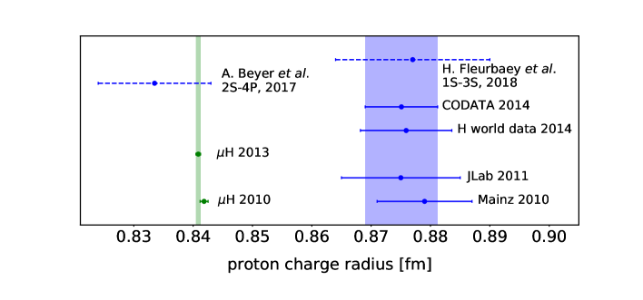
Figure 1: The present status of the proton radius puzzle: proton charge radius determinations from $\mu{\rm H}$ [1, 4] in comparison to the CODATA-2014 evaluation [5], data taken in Mainz [9] and at JLab [10] for electron scattering off the proton and results from world average ordinary hydrogen spectroscopy [5]. The latest hydrogen spectroscopy measurements by Beyer et al. [14] and Fleurbaey et al. [15] are also shown.

To date, no commonly accepted explanation exists. Very recently, two new measurements were performed based on spectroscopy of ordinary hydrogen, leading yet again to two contradicting results: the Garching experiment measured the $2S$–$4P$ transition frequency in $e$H yielding a small radius $r_{p}$ = 0.8335(95) fm [14] compatible with muonic hydrogen, while the Paris experiment examined $1S$–$3S$ transition frequency in $e$H obtaining $r_{p}$=0.877(13) fm [15], in very good agreement with the current CODATA-recommended value. The present situation with all the above mentioned results is depicted in Fig. 1. While this picture may suggest that systematic uncertainties in the various experiments need to be revisited, it is fair to say that the proton radius puzzle is yet to be solved and further investigations are needed.

To understand this discrepancy, new experiments have been proposed to measure precisely the electron-proton scattering at low momentum transfer down to $Q^{2}\sim 10^{-4}~{}(\rm{GeV/c})^{2}$ [16, 17, 18] and to investigate the low-$Q^{2}$ muon-proton elastic scattering in the MUSE experiment [19, 20]. An alternative approach is to study the mean-square charge radii $r_{nucl}$ of other light nuclei by measuring Lamb shifts in muonic atoms with different nuclear charges or mass numbers, such as muonic hydrogen isotopes ($\mu^{2}{\rm H}$ and $\mu^{3}{\rm H}$) and muonic helium ions ($\mu^{3}{\rm He}^{+}$ and $\mu^{4}{\rm He}^{+}$). Through a systematic comparison between $r_{nucl}$ extracted from experiments involving, respectively, electron-nucleus and muon-nucleus systems, one can test whether the discrepancy persists or is enhanced in systems with different number of protons $Z$, number of neutrons $N$, or different mass number $A=Z+N$. The CREMA collaboration at PSI has started to perform a series of Lamb shifts experiments in light muonic atoms [21]. Results on $\mu^{2}{\rm H}$ lead to the discovery of a deuteron-radius puzzle [22]. Results on helium isotopes will be released in the near future.

In the Lamb shift measurements, the accuracy in determining $r_{nucl}$ relies not only on the experimental precision, but also on how accurately one can calculate quantum electro-dynamics (QED) and nuclear-structure corrections. In light muonic atoms, unlike their electronic counter parts, QED corrections to the Lamb shifts are dominated by vacuum polarization rather than vertex corrections and the level ordering of the 2$S$ and 2$P$ states is reversed. Owing to the heavier mass, the muon orbits much closer to the nucleus than does the electron, thus nuclear-structure corrections are considerably larger than in electronic atoms [23, 24]. The Lamb shift $\delta_{\rm LS}$ in a muonic atom/ion with nuclear charge $Z$ can be generally related to the charge radius of a nucleus $r_{nucl}$ (in units of $\hbar=c=1$) by

$$\delta_{\rm LS}=\delta_{\rm QED}+\mathcal{A}_{\rm OPE}\,r^{2}_{nucl}+\delta_{\rm TPE},$$ (1)

where the $\delta_{\rm QED}$ term is composed mainly of QED photon vacuum polarization, muon self energy, and relativistic recoil corrections, whose dominant effect, i.e., the Uehling term, is of order $\alpha(Z\alpha)^{2}$ [25] with $\alpha$ denoting the fine-structure constant. Beyond the leading contribution, various QED corrections of higher orders (e.g., up to $(Z\alpha)^{6}$, $\alpha^{2}(Z\alpha)^{4}$, $\cdots$) have been calculated by many groups to very good accuracy (see Refs. [24, 25] for reviews). The other two terms in Eq. (1) are nuclear-structure corrections. The term proportional to $r^{2}_{nucl}$ is dominated by the exchange of one photon between the muon and the nucleus (Fig. 2), where the nuclear electric form factor is inserted into the photon-nucleus vertex. Such dominant effect determines the coefficient $\mathcal{A}_{\rm OPE}\approx m_{r}^{3}(Z\alpha)^{4}/12$, where $m_{r}=m_{\mu}M_{A}/(m_{\mu}+M_{A})$ is the reduced mass in the muon-nucleus center of mass system, with the nuclear mass denoted by $M_{A}$. Higher-order corrections to $\mathcal{A}_{\rm OPE}$ from relativistic, QED and nuclear finite-size effects have been calculated to great accuracy (see Refs. [24, 26] for reviews).

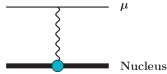
Figure 2: The muon-nucleus one-photon exchange.

The $\delta_{\rm TPE}$, which is of order $(Z\alpha)^{5}$, originates from the two-photon exchange (TPE) contribution (Fig. 3) and can be separated into elastic and inelastic parts, $\delta_{\rm TPE}=\delta_{\rm Zem}+\delta_{\rm pol}$. The elastic part $\delta_{\rm Zem}$ was derived by Friar as the dominant nuclear finite-size effect [26]. $\delta_{\rm Zem}$ is proportional to the third electric Zemach moment [27], also called Friar moment, which is expressed as an integral of the nuclear charge density $\rho_{E}(\bm{R})$:

$$\delta_{\rm Zem}=-\frac{m_{r}^{4}}{24}(Z\alpha)^{5}\int\int d^{3}{R}d^{3}{R}^{\prime}\left|\bm{R}-\bm{R}^{\prime}\right|^{3}\rho_{E}(\bm{R})\rho_{E}(\bm{R}^{\prime}).$$ (2)

The inelastic part $\delta_{\rm pol}$ is called the nuclear polarizability and reflects the excitation and deexcitation of the nucleus/nucleon through two-photon-exchange interaction with the muon shown in Fig. 3. Due to the energy-scale separation between the nuclear and the nucleon excitation energies, $\delta_{\rm pol}$ can be further separated into a nuclear contribution $\delta^{A}_{\rm pol}$ related to the few-nucleon dynamics and a hadronic part $\delta^{N}_{\rm pol}$, related to the intrinsic nucleon dynamics. Their effects can be studied independently using effective theories at different scales.

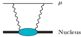
Figure 3: The muon-nucleus two-photon exchange.

To understand the physical meaning of $\delta^{A}_{\rm pol}$, one can naively imagine that the protons are pulled away from the nuclear center of mass due to the Coulomb attractions to the lepton, thus generating mostly nuclear dipole-excited states. Such a distorted charge distribution then tries to follow the orbiting lepton, similar to Earth’s equipotential tidal bulges lagging behind the Moon [28].

The spectroscopic measurements of Lamb shift $\delta_{\rm LS}$ can reach very high accuracy, and so can the calculation of $\delta_{\rm QED}$. Therefore, a key ingredient for extracting $r_{nucl}$ from Eq. (1) is the accurate determination of $\delta_{\rm TPE}$. Ab initio nuclear-structure calculations of $\delta_{\rm TPE}$ have already impacted this field, as we shall present in this review. A precision of the order of a few percent can be reached, which is presently better than any other method based on phenomenology or experimental extractions of the $\delta_{\rm TPE}$ contribution.

Table 1: Experimental uncertainty in the measured Lamb-shift energy of muonic atoms compared to the theoretical uncertainty in ab initio calculations of $\delta_{\rm TPE}$. Data taken from Refs. [4, 22, 29, 30, 31, 32, 33, 34].

	Experiment	Theory
$\mu{\rm H}$	2.3 $\mu$eV	2 $\mu$eV
$\mu^{2}{\rm H}$	0.034 meV	0.05 meV
$\mu^{3}\rm{He}^{+}$	0.08 meV	0.4 meV
$\mu^{4}\rm{He}^{+}$	0.06 meV	0.4 meV

To appreciate the importance of determining nuclear-structure corrections and reducing their uncertainties, the experimental uncertainty in the Lamb shift energy measurements is compared in Table 1 to the theoretical uncertainties in $\delta_{\rm TPE}$. One can see that for the $\mu{\rm H}$ case both uncertainties are of the same order of magnitude. However, for $\mu^{2}{\rm H}$, $\mu^{3}$He⁺ and $\mu^{4}$He⁺ the ratio between them is dramatically increased. This indicates, that for light muonic atoms TPE corrections constitute the real bottleneck to exploit the experimental precision in the extraction of the charge radius. It is important to note that ab initio nuclear-structure calculations performed for muonic atoms from $\mu^{2}{\rm H}$ to $\mu^{4}$He⁺ have so far provided the most precise determination of $\delta_{\rm TPE}$, substantially reducing the uncertainties with respect to other methods and approaches. Moreover, regardless of the source of the proton radius discrepancy, the TPE correction is a necessary theoretical input that determines the attainable precision of nuclear charge radii extracted from spectroscopic measurements of muonic atoms.

The purpose of this review is to present a thorough derivation of the formalism used to calculate $\delta_{\rm TPE}$ with ab initio methods and to compare our recent results to other approaches, emphasizing the reduction in uncertainty obtained by using first principle nuclear physics techniques.

The review is structured as follows. Section 2 will be dedicated to the theoretical formalism. In Section 3 we briefly outline the few-body methods used in our computations and in Section 4 we explain how we estimate theoretical uncertainties. Finally, in Section 5 we discuss our results in the context of other approaches and of the newly risen experimental questions, before drawing conclusions in Section 6.

2 Theoretical formulation

2.1 Summary of formulas

For readers interested only in the final expressions of the formulas, we present here a prescription for computing nuclear-structure corrections to the $2S$ state energy of a hydrogen-like muonic atom (or ion), in which a single muon orbits a nucleus ${}^{A}_{Z}{\rm X}$ with charge number $Z$ and mass number $A$. The $2P$ state is less influenced by the nucleus, due to the fact that the muon $2P$ wave function overlaps much less with the nucleus.

The entire two-photon exchange contribution in a muonic atom, $\delta_{\rm TPE}$, contains corrections from the nucleus structure $\delta_{\rm TPE}^{A}$ and the intrinsic nucleon structure $\delta_{\rm TPE}^{N}$, each of which is further separated into elastic component (Zemach contribution) and inelastic one (polarizability). Therefore, these four contributing terms are categorized in two ways:

$$\delta_{\rm TPE} = \delta_{\rm TPE}^{A}+\delta_{\rm TPE}^{N}=\left[\delta_{\rm pol}^{A}+\delta_{\rm Zem}^{A}\right]+\left[\delta_{\rm pol}^{N}+\delta_{\rm Zem}^{N}\right]{,}$$ (3a)

$$\delta_{\rm TPE} = \delta_{\rm Zem}\,+\delta_{\rm pol}\;\;=\left[\delta_{\rm Zem}^{A}+\delta_{\rm Zem}^{N}\right]+\left[\delta_{\rm pol}^{A}+\delta_{\rm pol}^{N}\right]{.}$$ (3b)

The nuclear polarizability, $\delta_{\rm pol}^{A}$, consists of four major contributions: non-relativistic $\delta_{\rm pol}^{\rm NR}$ (Section 2.2), Coulomb distortion $\delta_{\rm pol}^{\rm C}$ (Section 2.3), relativistic $\delta_{\rm pol}^{\rm R}$ (Section 2.4), and nucleon-size $\delta_{\rm pol}^{\rm NS}$ (Section 2.5) corrections. The four parts of $\delta_{\rm pol}^{A}$, together with $\delta_{\rm Zem}^{A}$, are further divided into smaller fragments, which are shown in the square brackets of Eqs. (3da, 3db).

$$\delta_{\rm pol}^{A} = \delta_{\rm pol}^{\rm NR}+\delta_{\rm pol}^{\rm C}+\delta_{\rm pol}^{\rm R}+\delta_{\rm pol}^{\rm NS}$$ (3da)

$$= \left[\delta^{(0)}_{D1}+(\delta^{(1)}_{R3}+\delta^{(1)}_{Z3})+(\delta^{(2)}_{R^{2}}+\delta^{(2)}_{Q}+\delta^{(2)}_{D1D3})\right]+\left[\delta^{(0)}_{C}\right]$$

$$+\left[\delta^{(0)}_{L}+\delta^{(0)}_{T}+\delta^{(0)}_{M}\right]+\left[\delta^{(1)}_{R1}+\delta^{(1)}_{Z1}+\delta^{(2)}_{NS}\right]{,}$$

$$\delta_{\rm Zem}^{A} = -\left[\delta^{(1)}_{Z3}+\delta^{(1)}_{Z1}\right]{.}$$ (3db)

Each term in Eqs. (3da) and (3db) will be explained in the following sub-sections. Here, we list the expressions for calculating each term:

$$\delta^{(0)}_{D1} = -\frac{16\pi^{2}}{9}(Z\alpha)^{2}\phi^{2}(0)\int^{\infty}_{0}d\omega\sqrt{\frac{2m_{r}}{\omega}}S_{D_{1}}(\omega){,}$$ (3dea)

$$\delta^{(1)}_{R3} = -\frac{\pi}{3}m_{r}(Z\alpha)^{2}\phi^{2}(0)\int\int d^{3}Rd^{3}R^{\prime}|\bm{R}-\bm{R}^{\prime}|^{3}\rho_{0}^{pp}(\bm{R},\bm{R}){,}$$ (3deb)

$$\delta^{(1)}_{Z3} = \hskip 12.91663pt\frac{\pi}{3}m_{r}(Z\alpha)^{2}\phi^{2}(0)\int\int d^{3}Rd^{3}R^{\prime}|\bm{R}-\bm{R}^{\prime}|^{3}\rho_{0}^{p}(\bm{R})\rho_{0}^{p}(\bm{R}^{\prime}){,}$$ (3dec)

$$\delta^{(2)}_{R^{2}} = \hskip 12.91663pt\frac{4\pi}{9}m_{r}^{2}(Z\alpha)^{2}\phi^{2}(0)\int^{\infty}_{0}d\omega\sqrt{\frac{\omega}{2m_{r}}}S_{R^{2}}(\omega){,}$$ (3ded)

$$\delta^{(2)}_{Q} = \hskip 12.91663pt\frac{64}{225}\pi^{2}m_{r}^{2}(Z\alpha)^{2}\phi^{2}(0)\int^{\infty}_{0}d\omega\sqrt{\frac{\omega}{2m_{r}}}S_{Q}(\omega){,}$$ (3dee)

$$\delta^{(2)}_{D1D3} = -\frac{64}{45}\pi^{2}m_{r}^{2}(Z\alpha)^{2}\phi^{2}(0)\int^{\infty}_{0}d\omega\sqrt{\frac{\omega}{2m_{r}}}S_{D_{1}D_{3}}(\omega){,}$$ (3def)

$$\delta_{C}^{(0)} = -\frac{16\pi^{2}}{9}(Z\alpha)^{3}\phi^{2}(0)\int_{0}^{\infty}d\omega\frac{m_{r}}{\omega}\ln\frac{2(Z\alpha)^{2}m_{r}}{\omega}\,S_{D_{1}}(\omega){,}$$ (3deg)

$$\delta_{L}^{(0)} = \hskip 12.91663pt\frac{32\pi}{9}(Z\alpha)^{2}\phi^{2}(0)\int^{\infty}_{0}d\omega\,\mathcal{F}_{L}(\omega/m_{r})S_{D_{1}}(\omega){,}$$ (3deh)

$$\delta_{T}^{(0)} = \hskip 12.91663pt\frac{16\pi}{9}(Z\alpha)^{2}\phi^{2}(0)\int^{\infty}_{0}d\omega\,\mathcal{F}_{T}(\omega/m_{r})S_{D_{1}}(\omega){,}$$ (3dei)

$$\delta_{M}^{(0)} = \hskip 12.91663pt\frac{1}{3m_{p}^{2}}(Z\alpha)^{2}\phi^{2}(0)\int^{\infty}_{0}d\omega\,\mathcal{F}_{M}(\omega/m_{r})S_{M_{1}}(\omega){,}$$ (3dej)

$$\delta^{(1)}_{R1} = -8\pi m_{r}(Z\alpha)^{2}\phi^{2}(0)\int\int d^{3}Rd^{3}R^{\prime}|\bm{R}-\bm{R}^{\prime}|\left[\frac{2}{\beta^{2}}\rho_{0}^{pp}(\bm{R},\bm{R}^{\prime})-\lambda\rho_{0}^{np}(\bm{R},\bm{R}^{\prime})\right]{,}$$ (3dek)

$$\delta^{(1)}_{Z1} = \hskip 12.91663pt8\pi m_{r}(Z\alpha)^{2}\phi^{2}(0)\int\int d^{3}Rd^{3}R^{\prime}|\bm{R}-\bm{R}^{\prime}|\rho_{0}^{p}(\bm{R})\left[\frac{2}{\beta^{2}}\rho_{0}^{p}(\bm{R}^{\prime})-\lambda\rho_{0}^{n}(\bm{R}^{\prime})\right]{,}$$ (3del)

$$\delta^{(2)}_{NS} = -\frac{128}{9}\pi^{2}m_{r}^{2}(Z\alpha)^{2}\phi^{2}(0)\left[\frac{2}{\beta^{2}}+\lambda\right]\int^{\infty}_{0}d\omega\sqrt{\frac{\omega}{2m_{r}}}S_{D_{1}}(\omega){.}$$ (3dem)

Here, $\phi^{2}(0)=(m_{r}Z\alpha)^{3}/8\pi$ is the norm of the muonic $2S$-state wave function. The parameters $\beta$ and $\lambda$ are defined as $\beta=\sqrt{12/r_{p}^{2}}$ and $\lambda=-r_{n}^{2}/6$, with $r_{p}$ and $r_{n}$ denoting the proton and neutron charge radius. The expressions above are in general energy-weighted integrations of nuclear electromagnetic response functions, called sum rules. Besides power-law and logarithmic energy weights, expressions of more complicated ones, i.e., $\mathcal{F}_{L}$, $\mathcal{F}_{T}$, and $\mathcal{F}_{M}$, are given respectively in Eqs. (3degmabbhbtdfdjdkdx, 3degmabbhbtdfdjdken, 3degmabbhbtdfdjdkeoeu). A response function $S_{O}$ is defined as

$$S_{O}(\omega)=\frac{1}{2J_{0}+1}\operatorname*{\mathchoice{\ooalign{$\displaystyle\sum$\cr$\displaystyle\int$\cr}}{\ooalign{\raisebox{0.14pt}{\scalebox{0.7}{$\textstyle\sum$}}\cr$\textstyle\int$\cr}}{\ooalign{\raisebox{0.2pt}{\scalebox{0.6}{$\scriptstyle\sum$}}\cr$\scriptstyle\int$\cr}}{\ooalign{\raisebox{0.2pt}{\scalebox{0.6}{$\scriptstyle\sum$}}\cr$\scriptstyle\int$\cr}}}\limits_{N\neq N_{0},J}|\langle N_{0}J_{0}||\hat{O}||NJ\rangle|^{2}\delta(\omega-\omega_{N}){,}$$ (3def)

where $\operatorname*{\mathchoice{\ooalign{$\displaystyle\sum$\cr$\displaystyle\int$\cr}}{\ooalign{\raisebox{0.14pt}{\scalebox{0.7}{$\textstyle\sum$}}\cr$\textstyle\int$\cr}}{\ooalign{\raisebox{0.2pt}{\scalebox{0.6}{$\scriptstyle\sum$}}\cr$\scriptstyle\int$\cr}}{\ooalign{\raisebox{0.2pt}{\scalebox{0.6}{$\scriptstyle\sum$}}\cr$\scriptstyle\int$\cr}}}$ indicates the sum of nuclear excited states (both discrete and continuum), $\hat{O}$ is an electromagnetic operator, and $\langle N_{0}J_{0}||\hat{O}||NJ\rangle$ denotes a reduced matrix element. $\omega_{N}$ is the excitation energy between nuclear states $|NJ\rangle$ and $|N_{0}J_{0}\rangle$. Readers can find the specific response functions $S_{D_{1}}$ in Eq. (3degmabbe), $S_{R^{2}}$ in Eq. (3degmabbhbti), $S_{Q}$ in Eq. (3degmabbhbtr), $S_{D_{1}D_{3}}$ in Eq. (3degmabbhbtaa), and $S_{M_{1}}$ in Eq. (3degmabbhbtdfdjdkeoer).

The one- and two-body point-nucleon densities are defined by

$$\rho_{0}^{c}(\bm{R}) = \langle N_{0}|\frac{1}{Z}\sum_{a}^{A}\delta(\bm{R}-\bm{R}_{a})\hat{e}_{c,a}|N_{0}\rangle{,}$$ (3dega)

$$\rho_{0}^{cc^{\prime}}(\bm{R},\bm{R}^{\prime}) = \langle N_{0}|\frac{1}{Z^{2}}\sum_{ab}^{A}\delta(\bm{R}-\bm{R}_{a})\delta(\bm{R}^{\prime}-\bm{R}_{b})\hat{e}_{c,a}\hat{e}_{c^{\prime},b}|N_{0}\rangle{,}$$ (3degb)

where $c,c^{\prime}$ equals $p$ or $n$. $\hat{e}_{p,a}$ and $\hat{e}_{n,a}$ are the proton and neutron projection isospin operators, defined as

$$\hat{e}_{p,a}=(1+\hat{\tau}_{z,a})/2,\quad\quad\hat{e}_{n,a}=(1-\hat{\tau}_{z,a})/2~{},$$ (3degh)

where $\hat{\tau}_{z,a}=\pm 1$ with the sign determined by the $a$th nucleon being a proton or neutron.

Eq. (3dea), calculated in Section 2.2.1, represents the leading contribution to the non-relativistic polarizability effect $\delta_{\rm pol}^{\rm NR}$. Eqs. (3deb, 3dec) are the sub-leading corrections to $\delta_{\rm pol}^{\rm NR}$, given in Section 2.2.2. Eqs. (3ded, 3dee, 3def) form the sub-sub-leading contributions to $\delta_{\rm pol}^{\rm NR}$, provided in Section 2.2.3. Eq. (3deg) represents the Coulomb-distortion correction, given in Section 2.3. Eqs. (3deh, 3dei, 3dej) are the relativistic corrections, which are derived in Section 2.4. Eqs. (3dek, 3del) and Eq. (3dem) show the leading and subleading nucleon-size effects, which can be found in Section 2.5.

2.2 Non-relativistic calculations

The muonic atom (or ion) is a hydrogen-like system consisting of a muon and a nucleus. The non-relativistic Hamiltonian of the muonic atom has three components, i.e., the nuclear Hamiltonian $H_{\rm nucl}$, the muon Hamiltonian $H_{\mu}$, and the nuclear-structure correction $\Delta H$:

$$H=H_{\rm nucl}+H_{\mu}+\Delta H{.}$$ (3degi)

$H_{\rm nucl}$ describes the internal structure of a nucleus ${}_{Z}^{A}{\rm X}$. It is written in terms of nucleon degrees of freedom, and the nuclear potential is represented by two- and three-nucleon interactions. We use a shorthand notation $|N\rangle$ to denote the $N$th nuclear eigenstate:

$$H_{\rm nucl}|N\rangle=E_{N}|N\rangle{,}$$ (3degj)

with $E_{N}$ indicating the corresponding eigenenergy. $|N\rangle$ refers to both discrete and continuum states, whose quantum numbers, such as the total angular momentum $J$ and its $z$-component $M$, are omitted for simplicity. In later cases, we also refer to $|N\rangle$ as $|NJ\rangle$ or $|NJM\rangle$, when specific quantum numbers are required. For the ground state, whose energy, total angular momentum, and $z$-component are respectively $E_{N_{0}}$, $J_{0}$ and $M_{0}$, we refer to it as $|N_{0}\rangle$, $|N_{0}J_{0}\rangle$ or $|N_{0}J_{0}M_{0}\rangle$.

$H_{\mu}$ is the muon Hamiltonian. The muon is bound to a point-like nucleus by an attractive Coulomb interaction. In the non-relativistic limit, $H_{\mu}$ is written as

$$H_{\mu}=\frac{q^{2}}{2m_{r}}-\frac{Z\alpha}{r}{,}$$ (3degk)

where $q$ and $r$ are the relative momentum and distance between the muon and the nucleus. The eigenenergy $\epsilon_{\mu}$ of the Hamiltonian $H_{\mu}$, leads to the unperturbed (not necessarily ground-state) atomic spectrum; while $|\mu\rangle$ indicates the corresponding eigenstate. When atomic quantum numbers need to be specified, we use a full notation $|{\mu}_{n\ell m}\rangle$ (or $|{\mu}_{n\ell}\rangle$) to specify the principle ($n$), orbital ($\ell$) and magnetic ($m$) quantum numbers of an atomic state, whose coordinate-space representation is,

$$\langle\bm{r}|{\mu}_{n\ell m}\rangle=\phi_{n}(0)\left(\frac{4\pi}{2\ell+1}\right)^{1/2}R_{n\ell}(r)\;Y_{\ell m}(\hat{r}){,}$$ (3degl)

where $\phi_{n}(0)$ is the wave-function normalization constant. Since we focus on the Lamb shift in muonic atoms, we take only $n=2$ in this article, and drop the subscript in $\phi_{2}(0)$ for simplicity. So we have $\phi(0)=\nu^{3/2}/\sqrt{\pi}$, with $\nu=m_{r}Z\alpha/2$. The unperturbed atomic energy, $\epsilon_{\mu}=-m_{r}(Z\alpha)^{2}/8$, is degenerate in unperturbed $2S$ and $2P$ states, whose radial functions are respectively

$$R_{20}(r) = (1-\nu r)\exp\left(-\nu r\right){,}$$ (3degma)

$$R_{21}(r) = \nu r\exp\left(-\nu r\right){.}$$ (3degmb)

$\Delta H$ in Eq. (3degi) describes the correction to the muon-nucleus point Coulomb interaction from the charge distribution of the nucleus. In this section, the nucleus is approximated by a system consisting of point-like protons (charge $1$) and neutrons (charge $0$). Therefore, $\Delta H$ represents the sum of Coulomb interactions of the muon with each individual proton, located at a position $\bm{R}_{a}$ (or distance $R_{a}=|\bm{R_{a}}|$) from the nuclear center of mass, subtracted by the point Coulomb potential,

$$\eqalign{\Delta H=\sum\limits_{a}^{Z}\Delta V(\bm{r},\bm{R}_{a}){,}\\ \Delta V(\bm{r},\bm{R})=-\alpha\left(\frac{1}{|\bm{r}-\bm{R}|}-\frac{1}{r}\right){.}}$$ (3degmn)

The function $\Delta V$ is localized around the nucleus, and vanishes when the limit $r\gg R$ is approached. Eq. (3degmn) does not account for the internal nucleonic structure, whose correction to $\Delta H$ enters at higher orders. We will discuss the finite nucleon-size correction in Section 2.5.

Since $\Delta H$ scales with $Z\alpha$, which is small in light muonic atoms, we use perturbation theory to evaluate $\Delta H$’s correction to the muonic atom spectrum. The $Z\alpha$-dependence of $|\mu\rangle$ and $\Delta H$ indicates that nuclear-structure corrections from the $k$th-order perturbation theory are sized with $(Z\alpha)^{k+3}$ for the $2S$ state and $(Z\alpha)^{k+5}$ for the $2P$ state. The first-order perturbation theory leads to the expectation value $\langle N_{0}\mu|\Delta H|N_{0}\mu\rangle$, and is represented by the muon-nucleus one-photon exchange process depicted in Figure 2. As derived in [26], its contribution to the $2S$ state is approximately $m_{r}^{3}(Z\alpha)^{4}r_{\rm nucl}^{2}/12$; while corrections to the $2P$-state are of order $(Z\alpha)^{6}$.

In this article, we limit the discussions to second-order perturbation theory. It is of order $(Z\alpha)^{5}$, and is characterized by the two-photon exchange process depicted in Figure 3. Depending on whether the nucleus remains in the ground state between the exchanged photons, corrections are further divided into elastic and inelastic parts. The nuclear-elastic part is called nuclear finite-size effect, which was calculated by Friar [26] . In the two-photon exchange process, the elastic part corresponds to the elastic nuclear Zemach contribution $\delta_{\rm Zem}^{A}$. The nuclear-inelastic part is named nuclear polarizability effect, $\delta_{\rm pol}^{A}$, for which the nucleus is excited by absorbing a photon and is then de-excited by subsequently emitting another photon.

The nuclear polarizability $\delta_{\rm pol}^{A}$ is calculated in second-order perturbation theory by

$$\delta_{\rm pol}^{A}=\langle N_{0}{\mu}|\Delta H\,G\,\Delta H|N_{0}{\mu}\rangle{,}$$ (3degmo)

where $G$ is the Green’s function represented in a complete basis except for the nuclear ground state, i.e., $1-|N_{0}\rangle\langle N_{0}|$. Using closure, $G$ is given by

$$G=-\operatorname*{\mathchoice{\ooalign{$\displaystyle\sum$\cr$\displaystyle\int$\cr}}{\ooalign{\raisebox{0.14pt}{\scalebox{0.7}{$\textstyle\sum$}}\cr$\textstyle\int$\cr}}{\ooalign{\raisebox{0.2pt}{\scalebox{0.6}{$\scriptstyle\sum$}}\cr$\scriptstyle\int$\cr}}{\ooalign{\raisebox{0.2pt}{\scalebox{0.6}{$\scriptstyle\sum$}}\cr$\scriptstyle\int$\cr}}}\limits_{N\neq N_{0}}\frac{|N\rangle\langle N|}{H_{\mu}+\omega_{N}-\epsilon_{\mu}}{,}$$ (3degmp)

where $\operatorname*{\mathchoice{\ooalign{$\displaystyle\sum$\cr$\displaystyle\int$\cr}}{\ooalign{\raisebox{0.14pt}{\scalebox{0.7}{$\textstyle\sum$}}\cr$\textstyle\int$\cr}}{\ooalign{\raisebox{0.2pt}{\scalebox{0.6}{$\scriptstyle\sum$}}\cr$\scriptstyle\int$\cr}}{\ooalign{\raisebox{0.2pt}{\scalebox{0.6}{$\scriptstyle\sum$}}\cr$\scriptstyle\int$\cr}}}$ indicates the summation of both discrete and continuum nuclear states, and $\omega_{N}=E_{N}-E_{N_{0}}$.

As is proven in Section 2.3, $\delta_{\rm pol}^{A}$ contributes equally to the two hyperfine states associated with the $2S$ state. Here we simply set the muonic-atom state $|N_{0}\mu\rangle$ with nuclear and muonic parts decoupled, i.e., $|N_{0}\mu\rangle=|N_{0}\rangle|\mu\rangle$. By substituting Eqs. (3degmn) and (3degmp) into Eq. (3degmo), and using closure in muon’s coordinate-space, we have

$$\delta_{\rm pol}^{A} = -\sum_{ab}^{Z}\operatorname*{\mathchoice{\ooalign{$\displaystyle\sum$\cr$\displaystyle\int$\cr}}{\ooalign{\raisebox{0.14pt}{\scalebox{0.7}{$\textstyle\sum$}}\cr$\textstyle\int$\cr}}{\ooalign{\raisebox{0.2pt}{\scalebox{0.6}{$\scriptstyle\sum$}}\cr$\scriptstyle\int$\cr}}{\ooalign{\raisebox{0.2pt}{\scalebox{0.6}{$\scriptstyle\sum$}}\cr$\scriptstyle\int$\cr}}}_{N\neq N_{0}}\int\int d^{3}rd^{3}r^{\prime}\langle N_{0}|\Delta V(\bm{r},\bm{R}_{a})|N\rangle\langle{\mu}|\bm{r}\rangle$$ (3degmz)

$$\times\langle\bm{r}|\frac{1}{H_{\mu}+\omega_{N}-\epsilon_{\mu}}|\bm{r}^{\prime}\rangle\langle\bm{r}^{\prime}|{\mu}\rangle\langle N|\Delta V(\bm{r}^{\prime},\bm{R}_{b})|N_{0}\rangle{.}$$

It is useful to define the point-proton transition density function

$$\rho_{N}^{p}(\bm{R})=\langle N|\frac{1}{Z}\sum_{a}^{A}\delta(\bm{R}-\bm{R}_{a})\hat{e}_{p,a}|N_{0}\rangle{,}$$ (3degmaa)

with $\hat{e}_{p,a}$ defined in Eq. (3degh). $\rho_{N}^{p}$ satisfies the sum rules:

$$\int d^{3}R\,\rho_{N}^{p}(\bm{R})\hat{O}(\bm{R})=\frac{1}{Z}\sum_{a}^{Z}\langle N|\hat{O}(\bm{R}_{a})|N_{0}\rangle{,}$$ (3degmaba)

$$\int d^{3}R\,\rho_{N}^{p}(\bm{R})=\frac{1}{Z}\sum_{a}^{Z}\langle N|N_{0}\rangle=\delta_{NN_{0}}{,}$$ (3degmabb)

where $\hat{O}(\bm{R})$ is an arbitrary operator, and Eq. (3degmabb) indicates the orthonormal condition in nuclear states. One special case of Eq. (3degmaba) is the ground-state point-proton density $\rho_{0}^{p}(\bm{R})$ defined in Eq. (3dega), which is normalized by $\int d^{3}R\rho_{0}^{p}(\bm{R})=1$. Another case is that

$$\sum\limits_{a}^{Z}\langle N|\Delta V(\bm{r},\bm{R}_{a})|N_{0}\rangle=Z\int d^{3}R\,\rho^{p}_{N}(\bm{R})\,\Delta V(\bm{r},\bm{R}){.}$$ (3degmabac)

By substituting Eq. (3degmabac) into Eq. (3degmz), we have

$$\delta_{\rm pol}^{A}=\operatorname*{\mathchoice{\ooalign{$\displaystyle\sum$\cr$\displaystyle\int$\cr}}{\ooalign{\raisebox{0.14pt}{\scalebox{0.7}{$\textstyle\sum$}}\cr$\textstyle\int$\cr}}{\ooalign{\raisebox{0.2pt}{\scalebox{0.6}{$\scriptstyle\sum$}}\cr$\scriptstyle\int$\cr}}{\ooalign{\raisebox{0.2pt}{\scalebox{0.6}{$\scriptstyle\sum$}}\cr$\scriptstyle\int$\cr}}}_{N\neq N_{0}}\int d^{3}Rd^{3}R^{\prime}\rho_{N}^{p*}(\bm{R}){W}(\bm{R},\bm{R}^{\prime},\omega_{N})\rho_{N}^{p}(\bm{R}^{\prime}){,}$$ (3degmabad)

where ${W}$ is the muon matrix element

$${W}(\bm{R},\bm{R}^{\prime},\omega_{N}) = -Z^{2}\int d^{3}rd^{3}r^{\prime}\Delta V(\bm{r},\bm{R})\langle{\mu}|\bm{r}\rangle$$ (3degmabae)

$$\times\langle\bm{r}|\frac{1}{H_{\mu}+\omega_{N}-\epsilon_{\mu}}|\bm{r}^{\prime}\rangle\langle\bm{r}^{\prime}|{\mu}\rangle\Delta V(\bm{r}^{\prime},\bm{R}^{\prime}){.}$$

In the small $Z\alpha$ expansion, $\Delta V\propto\alpha$, $\langle\bm{r}|\mu_{20}\rangle\sim(Z\alpha)^{3/2}$ and $\langle\bm{r}|\mu_{21}\rangle\sim(Z\alpha)^{5/2}$. Therefore, ${W}$ in the atomic $2S$ state is of order $(Z\alpha)^{5}$; while that in the $2P$ state is of order $(Z\alpha)^{7}$. By considering the dominant polarizability contribution, which is of order $(Z\alpha)^{5}$, we neglect the atomic $2P$ state, and calculate $\delta_{\rm pol}^{A}$ only in the $2S$ state. In Eq. (3degmabae), we also omit $Z\alpha$-dependent pieces in $(H_{\mu}+\omega_{N}-\epsilon_{\mu})^{-1}$, whose contribution to $\delta_{\rm pol}^{A}$ is above $(Z\alpha)^{5}$. These approximations yield

$$\eqalign{\langle\bm{r}|\mu_{20}\rangle\rightarrow\phi(0)~{},&\langle\bm{r}|\mu_{21}\rangle\rightarrow 0{,}\\ H_{\mu}\rightarrow\frac{q^{2}}{2m_{r}}~{},&\epsilon_{\mu}\rightarrow 0{.}}$$ (3degmabah)

By inserting Eq. (3degmabah) into Eq. (3degmabae), and using closure in muon’s momentum space, we have

$${W}(\bm{R},\bm{R}^{\prime},\omega_{N}) = -\phi^{2}(0)Z^{2}\int\frac{d^{3}q}{(2\pi)^{3}}d^{3}rd^{3}r^{\prime}\Delta V(\bm{r},\bm{R})e^{i\bm{q}\cdot\bm{r}}\frac{1}{\frac{q^{2}}{2m_{r}}+\omega_{N}}e^{-i\bm{q}\cdot\bm{r}^{\prime}}\Delta V(\bm{r}^{\prime},\bm{R}^{\prime})$$ (3degmabai)

$$= -\phi^{2}(0)Z^{2}\int\frac{d^{3}q}{(2\pi)^{3}}\Delta\tilde{V}(\bm{q},\bm{R})\frac{1}{\frac{q^{2}}{2m_{r}}+\omega_{N}}\Delta\tilde{V}^{*}(\bm{q},\bm{R}^{\prime}){,}$$

where $\Delta\tilde{V}(\bm{q},\bm{R})$ is the Fourier transform of $\Delta V(\bm{r},\bm{R})$

$$\Delta\tilde{V}(\bm{q},\bm{R})=\int d^{3}r\Delta V(\bm{r},\bm{R})e^{i\bm{q}\cdot\bm{r}}=\frac{4\pi\alpha}{q^{2}}\left(1-e^{i\bm{q}\cdot\bm{R}}\right){.}$$ (3degmabaj)

By inserting Eq. (3degmabaj) into Eq. (3degmabai) and integrating over $d\hat{q}$, we have

$${W}(\bm{R},\bm{R}^{\prime},\omega_{N})=-16m_{r}(Z\alpha)^{2}\phi^{2}(0)\int_{0}^{\infty}\frac{dq}{q^{2}}\frac{1}{q^{2}+2m_{r}\omega_{N}}I(q,\bm{R},\bm{R}^{\prime}){,}$$ (3degmabak)

where the function $I(q,\bm{R},\bm{R}^{\prime})$ is given by

$$I(q,\bm{R},\bm{R}^{\prime})=1-\frac{\sin(qR)}{qR}-\frac{\sin(qR^{\prime})}{qR^{\prime}}+\frac{\sin(q|\bm{R}-\bm{R}^{\prime}|)}{q|\bm{R}-\bm{R}^{\prime}|}{.}$$ (3degmabal)

The first three terms in Eq. (3degmabal), which are independent on either $R$ or $R^{\prime}$, do not contribute to $\delta_{\rm pol}^{A}$, since they lead to terms in Eq. (3degmabad) proportional to $\int d^{3}R\,\rho_{N}^{p}(\bm{R})=0$ when $N\neq N_{0}$. Therefore, the irreducible part of ${W}$ yields

$${W}(\bm{R},\bm{R}^{\prime},\omega_{N})=-16m_{r}(Z\alpha)^{2}\phi^{2}(0)\int_{0}^{\infty}\frac{dq}{q^{2}}\frac{1}{q^{2}+2m_{r}\omega_{N}}\left[\frac{\sin(q|\bm{R}-\bm{R}^{\prime}|)}{q|\bm{R}-\bm{R}^{\prime}|}-1\right]{,}$$ (3degmabam)

where the constant $-1$ is added to cancel the divergence of the integrand at $q=0$.

After integrating over $q$, ${W}$ becomes

$${W}(\bm{R},\bm{R}^{\prime},\omega_{N})=-\frac{\pi}{m_{r}^{2}}(Z\alpha)^{2}\phi^{2}(0)\left(\frac{2m_{r}}{\omega_{N}}\right)^{3/2}\frac{1}{\eta}\left(e^{-\eta}-1+\eta-\frac{1}{2}\eta^{2}\right){,}$$ (3degmaban)

where $\eta\equiv\sqrt{2m_{r}\omega_{N}}|\bm{R}-\bm{R}^{\prime}|$ is a dimensionless operator. The quantity $|\bm{R}-\bm{R}^{\prime}|$ indicates the “virtual” distance that a proton inside the nucleus travels in the two-photon exchange process. We argue qualitatively using uncertainty principle, that $|\bm{R}-\bm{R}^{\prime}|$ scales inversely with the momentum boost $Q$ of the traveling proton. It is thus roughly related to the nuclear excitation energy by $\omega_{N}\sim Q^{2}/2m_{p}\sim(2m_{p})^{-1}|\bm{R}-\bm{R}^{\prime}|^{-2}$, with $m_{p}$ denoting the proton mass. Therefore, the parameter $\eta$ in Eq. (3degmaban) is approximately of order $\sqrt{m_{r}/m_{p}}\approx\sqrt{m_{\mu}/m_{p}}\ll 1$, and becomes a small parameter. Now we expand Eq. (3degmaban) in powers of $\eta$ and obtain

$${W}(\bm{R},\bm{R}^{\prime},\omega_{N}) = \frac{2\pi}{3}(Z\alpha)^{2}\phi^{2}(0)\sqrt{\frac{2m_{r}}{\omega_{N}}}$$ (3degmabao)

$$\times \left[|\bm{R}-\bm{R}^{\prime}|^{2}-\frac{1}{4}\sqrt{2m_{r}\omega_{N}}|\bm{R}-\bm{R}^{\prime}|^{3}+\frac{1}{10}m_{r}\omega_{N}|\bm{R}-\bm{R}^{\prime}|^{4}+\cdots~{}\right]{,}$$

where dots indicate higher-order terms omitted in the expansion. The three terms in the square brackets yield the leading $(0)$, sub-leading $(1)$, and sub-sub-leading $(2)$ non-relativistic contributions to $\delta_{\rm pol}^{A}$ in the $\eta$-expansion. Each term is further decomposed by

$$\eqalign{\delta_{\rm pol}^{\rm NR}&=\delta_{\rm NR}^{(0)}+\delta_{\rm NR}^{(1)}+\delta_{\rm NR}^{(2)}\\ &=[\delta^{(0)}_{D1}]+[\delta^{(1)}_{Z3}+\delta^{(1)}_{R3}]+[\delta^{(2)}_{R^{2}}+\delta^{(2)}_{Q}+\delta^{(2)}_{D1D3}]{.}}$$ (3degmabar)

In the remaining part of this section, we explain the derivation of each term and evaluate their contributions.

2.2.1 Leading non-relativistic contributions

In the $\eta$-expansion, the leading piece in Eq. (3degmabao) is proportional to $|\bm{R}-\bm{R}^{\prime}|^{2}$. It is expanded in spherical-harmonic basis by

$$|\bm{R}-\bm{R}^{\prime}|^{2}\rightarrow-\frac{8\pi}{3}RR^{\prime}\,Y_{1}(\hat{R})\cdot Y_{1}(\hat{R}^{\prime}){,}$$ (3degmabas)

where $Y_{l}$ denotes the rank-$l$ spherical harmonic tensor, and the scalar product is defined by $Y_{l}\cdot Y_{l}=\sum_{m=-l}^{l}Y_{lm}^{*}Y_{lm}$. $R^{2}$ and $R^{\prime 2}$ terms are dropped since they do not contribute to $\delta_{\rm pol}^{A}$ due to the orthogonality condition in Eq. (3degmabb). We separate Eq. (3degmabas) from the remaining pieces of $W$ in Eq. (3degmabao), and insert it into Eq. (3degmabad). By doing so, we obtain the leading non-relativistic polarizability contribution $\delta^{(0)}_{\rm NR}$, which equals to an electric dipole polarization, $\delta^{(0)}_{D1}$:

$$\delta^{(0)}_{D1} = -\frac{16\pi^{2}}{9}\alpha^{2}\phi^{2}(0)\sum_{ab}^{Z}\operatorname*{\mathchoice{\ooalign{$\displaystyle\sum$\cr$\displaystyle\int$\cr}}{\ooalign{\raisebox{0.14pt}{\scalebox{0.7}{$\textstyle\sum$}}\cr$\textstyle\int$\cr}}{\ooalign{\raisebox{0.2pt}{\scalebox{0.6}{$\scriptstyle\sum$}}\cr$\scriptstyle\int$\cr}}{\ooalign{\raisebox{0.2pt}{\scalebox{0.6}{$\scriptstyle\sum$}}\cr$\scriptstyle\int$\cr}}}_{N\neq N_{0},JM}\sqrt{\frac{2m_{r}}{\omega_{N}}}$$ (3degmabbc)

$$\times\langle N_{0}J_{0}M_{0}|R_{a}Y_{1}(\hat{R}_{a})|NJM\rangle\cdot\langle NJM|R_{b}Y_{1}(\hat{R}_{b})|N_{0}J_{0}M_{0}\rangle{.}$$

Where the full notation of a nuclear state $|NJM\rangle$ specifies the total angular momentum $J$ and its $z$-component $M$. For a given multipolarity-$l$ operator, $Y_{l}$, the allowed transition is constrained by $|J_{0}-l|\leq J\leq J_{0}+l$.

By defining an electric-dipole operator $\hat{D}_{1}=\frac{1}{Z}\sum_{a}^{Z}R_{a}Y_{1}(\hat{R}_{a})$, we rewrite Eq. (3degmabbc) based on the Wigner-Eckart theorem in Eq. (3degmabbhbtdfdjdkeoewfdfefffshj) as

$$\delta^{(0)}_{D1}=-\frac{16\pi^{2}}{9}(Z\alpha)^{2}\phi^{2}(0)\int^{\infty}_{0}d\omega\,\sqrt{\frac{2m_{r}}{\omega}}S_{D_{1}}(\omega){,}$$ (3degmabbd)

which is proportional to an electric dipole sum rule with an energy weight $\omega^{-1/2}$. $S_{D_{1}}$ is the electric dipole response function, defined in terms of reduced matrix elements

$$S_{D_{1}}(\omega)=\frac{1}{2J_{0}+1}\operatorname*{\mathchoice{\ooalign{$\displaystyle\sum$\cr$\displaystyle\int$\cr}}{\ooalign{\raisebox{0.14pt}{\scalebox{0.7}{$\textstyle\sum$}}\cr$\textstyle\int$\cr}}{\ooalign{\raisebox{0.2pt}{\scalebox{0.6}{$\scriptstyle\sum$}}\cr$\scriptstyle\int$\cr}}{\ooalign{\raisebox{0.2pt}{\scalebox{0.6}{$\scriptstyle\sum$}}\cr$\scriptstyle\int$\cr}}}\limits_{N\neq N_{0},J}|\langle N_{0}J_{0}||\hat{D}_{1}||NJ\rangle|^{2}\delta(\omega-\omega_{N}){.}$$ (3degmabbe)

2.2.2 Sub-leading non-relativistic contributions

$|\bm{R}-\bm{R}^{\prime}|^{3}$ in Eq. (3degmabao) leads to the part independent of $\omega_{N}$. Inserting this piece of ${W}$ into Eq. (3degmabad) yields the sub-leading non-relativistic contribution $\delta_{\rm NR}^{(1)}$:

$$\delta^{(1)}_{\rm NR}=-\frac{\pi(Z\alpha)^{2}}{3}m_{r}\phi^{2}(0)\int d^{3}R\int d^{3}R^{\prime}\,|\bm{R}-\bm{R}^{\prime}|^{3}\,\operatorname*{\mathchoice{\ooalign{$\displaystyle\sum$\cr$\displaystyle\int$\cr}}{\ooalign{\raisebox{0.14pt}{\scalebox{0.7}{$\textstyle\sum$}}\cr$\textstyle\int$\cr}}{\ooalign{\raisebox{0.2pt}{\scalebox{0.6}{$\scriptstyle\sum$}}\cr$\scriptstyle\int$\cr}}{\ooalign{\raisebox{0.2pt}{\scalebox{0.6}{$\scriptstyle\sum$}}\cr$\scriptstyle\int$\cr}}}_{N\neq N_{0}}\rho_{N}^{p*}(\bm{R})\rho_{N}^{p}(\bm{R}^{\prime}){.}$$ (3degmabbf)

Using closure $\operatorname*{\mathchoice{\ooalign{$\displaystyle\sum$\cr$\displaystyle\int$\cr}}{\ooalign{\raisebox{0.14pt}{\scalebox{0.7}{$\textstyle\sum$}}\cr$\textstyle\int$\cr}}{\ooalign{\raisebox{0.2pt}{\scalebox{0.6}{$\scriptstyle\sum$}}\cr$\scriptstyle\int$\cr}}{\ooalign{\raisebox{0.2pt}{\scalebox{0.6}{$\scriptstyle\sum$}}\cr$\scriptstyle\int$\cr}}}_{N\neq N_{0}}|N\rangle\langle N|=1-|N_{0}\rangle\langle N_{0}|$, the product-sum of point-proton transition density functions are separated into two ground-state expectation functions:

$$\operatorname*{\mathchoice{\ooalign{$\displaystyle\sum$\cr$\displaystyle\int$\cr}}{\ooalign{\raisebox{0.14pt}{\scalebox{0.7}{$\textstyle\sum$}}\cr$\textstyle\int$\cr}}{\ooalign{\raisebox{0.2pt}{\scalebox{0.6}{$\scriptstyle\sum$}}\cr$\scriptstyle\int$\cr}}{\ooalign{\raisebox{0.2pt}{\scalebox{0.6}{$\scriptstyle\sum$}}\cr$\scriptstyle\int$\cr}}}_{N\neq N_{0}}\rho_{N}^{p*}(\bm{R})\rho_{N}^{p}(\bm{R}^{\prime})=\rho_{0}^{pp}(\bm{R},\bm{R}^{\prime})-\rho_{0}^{p}(\bm{R})\rho_{0}^{p}(\bm{R}^{\prime}){,}$$ (3degmabbg)

where $\rho_{0}^{pp}$ is the point proton-proton correlation function defined in Eq. (3degb).

Therefore, the sub-leading contribution is separated into two parts, $\delta^{(1)}_{\rm NR}=\delta^{(1)}_{R3}+\delta^{(1)}_{Z3}$, which are defined respectively as

$$\delta^{(1)}_{R3} = -\frac{\pi}{3}m_{r}(Z\alpha)^{2}\phi^{2}(0)\int\int d^{3}Rd^{3}R^{\prime}|\bm{R}-\bm{R}^{\prime}|^{3}\,\rho_{0}^{(pp)}(\bm{R},\bm{R}){,}$$ (3degmabbha)

$$\delta^{(1)}_{Z3} = \frac{\pi}{3}m_{r}(Z\alpha)^{2}\phi^{2}(0)\int\int d^{3}Rd^{3}R^{\prime}|\bm{R}-\bm{R}^{\prime}|^{3}\,\rho_{0}^{p}(\bm{R})\rho_{0}^{p}(\bm{R}^{\prime}){.}$$ (3degmabbhb)

$\delta^{(1)}_{R3}$ is zero for hydrogen isotopes, but becomes finite for a nucleus with more than one proton. In the point-nucleon limit, the full charge distribution $\rho_{E}(\bm{R})$ is then replaced by the point-proton density $\rho_{0}^{p}(\bm{R})$. Therefore, $-\delta^{(1)}_{Z3}$ becomes exactly the elastic Zemach term, which is the elastic two-photon exchange contribution defined in Eq. (2). This cancellation was shown in Ref. [35] for TPE contributions in hydrogen-like atoms, and was later applied by Refs. [28, 36] to muonic atoms. However, when the internal nucleon charge density is considered, higher-order corrections to $\delta^{(1)}_{Z3}$ need to be evaluated. This is done in Section 2.5.

2.2.3 Sub-sub-leading non-relativistic contributions

The $|\bm{R}-\bm{R}^{\prime}|^{4}$ term in Eq. (3degmabao) yields the sub-sub-leading contribution in the $\eta$-expansion. It is represented in spherical-harmonic basis by

$$|\bm{R}-\bm{R}^{\prime}|^{4}\rightarrow\frac{10}{3}R^{2}R^{\prime 2}+\frac{32\pi}{15}R^{2}R^{\prime 2}Y_{2}(\hat{R})\cdot Y_{2}(\hat{R}^{\prime})-\frac{16\pi}{3}(R^{2}+R^{\prime 2})RR^{\prime}Y_{1}(\hat{R})\cdot Y_{1}(\hat{R}^{\prime}){,}\\$$

where $R^{4}$ and $R^{\prime 4}$ are dropped, since they do not contribute to $\delta_{\rm pol}^{A}$ due to the orthogonality condition in Eq. (3degmabb). By inserting the corresponding components of ${W}$ into Eq. (3degmabad), we have the sub-sub-leading non-relativistic contribution $\delta_{\rm NR}^{(2)}$

$$\delta^{(2)}_{\rm NR} = \frac{4\pi\alpha^{2}}{9}m_{r}^{2}\phi^{2}(0)\sum_{ab}^{Z}\operatorname*{\mathchoice{\ooalign{$\displaystyle\sum$\cr$\displaystyle\int$\cr}}{\ooalign{\raisebox{0.14pt}{\scalebox{0.7}{$\textstyle\sum$}}\cr$\textstyle\int$\cr}}{\ooalign{\raisebox{0.2pt}{\scalebox{0.6}{$\scriptstyle\sum$}}\cr$\scriptstyle\int$\cr}}{\ooalign{\raisebox{0.2pt}{\scalebox{0.6}{$\scriptstyle\sum$}}\cr$\scriptstyle\int$\cr}}}_{N\neq N_{0},JM}\sqrt{\frac{\omega_{N}}{2m_{r}}}\Bigl{[}\langle N_{0}J_{0}M_{0}|R^{2}_{a}|NJM\rangle\langle NJM|R^{2}_{b}|N_{0}J_{0}M_{0}\rangle$$ (3degmabbhbr)

$$+\frac{16\pi}{25}\langle N_{0}J_{0}M_{0}|R^{2}_{a}Y_{2}(\hat{R}_{a})|NJM\rangle\cdot\langle NJM|R^{2}_{b}Y_{2}(\hat{R}_{b})|N_{0}J_{0}M_{0}\rangle$$

$$-\frac{8\pi}{5}\left(\langle N_{0}J_{0}M_{0}|R^{3}_{a}Y_{1}(\hat{R}_{a})|NJM\rangle\cdot\langle NJM|R_{b}Y_{1}(\hat{R}_{b})|N_{0}J_{0}M_{0}\rangle+{\rm c.c.}\right)\Bigr{]}{.}$$

For simplicity, we define a monopole operator $\hat{R}^{2}\equiv\frac{1}{Z}\sum_{a}^{Z}R^{2}_{a}$, a quadrupole operator $\hat{Q}_{2}=\frac{1}{Z}\sum_{a}^{Z}R^{2}_{a}Y_{2}(\hat{R}_{a})$, and a new rank-$1$ operator $\hat{D}_{3}=\frac{1}{Z}\sum_{a}^{Z}R_{a}^{3}Y_{1}(\hat{R}_{a})$. Based on the Wigner-Eckart theorem in Eqs. (3degmabbhbtdfdjdkeoewfdfefffshi, 3degmabbhbtdfdjdkeoewfdfefffshj), we rewrite $\delta^{(2)}_{\rm NR}$ as a combination of three electric multipole sum rules

$$\delta^{(2)}_{\rm NR} = \delta^{(2)}_{R^{2}}+\delta^{(2)}_{Q}+\delta^{(2)}_{D1D3}$$ (3degmabbhbs)

$$= \frac{4\pi}{9}m_{r}^{2}(Z\alpha)^{2}\phi^{2}(0)\int^{\infty}_{0}d\omega\,\sqrt{\frac{\omega}{2m_{r}}}\left[S_{R^{2}}(\omega)+\frac{16\pi}{25}S_{Q}(\omega)-\frac{16\pi}{5}S_{D_{1}D_{3}}(\omega)\right]{,}$$

where $S_{R^{2}}$, $S_{Q}$, and $S_{D_{1}D_{3}}$ are respectively the electric monopole, quadrupole, and $D_{1}D_{3}$-interference response functions. They are defined by

$$S_{R^{2}}(\omega) = \frac{1}{2J_{0}+1}\operatorname*{\mathchoice{\ooalign{$\displaystyle\sum$\cr$\displaystyle\int$\cr}}{\ooalign{\raisebox{0.14pt}{\scalebox{0.7}{$\textstyle\sum$}}\cr$\textstyle\int$\cr}}{\ooalign{\raisebox{0.2pt}{\scalebox{0.6}{$\scriptstyle\sum$}}\cr$\scriptstyle\int$\cr}}{\ooalign{\raisebox{0.2pt}{\scalebox{0.6}{$\scriptstyle\sum$}}\cr$\scriptstyle\int$\cr}}}_{N\neq N_{0},J}|\langle N_{0}J_{0}||\hat{R}^{2}||NJ\rangle|^{2}\delta(\omega-\omega_{N}){,}$$ (3degmabbhbti)

$$S_{Q}(\omega) = \frac{1}{2J_{0}+1}\operatorname*{\mathchoice{\ooalign{$\displaystyle\sum$\cr$\displaystyle\int$\cr}}{\ooalign{\raisebox{0.14pt}{\scalebox{0.7}{$\textstyle\sum$}}\cr$\textstyle\int$\cr}}{\ooalign{\raisebox{0.2pt}{\scalebox{0.6}{$\scriptstyle\sum$}}\cr$\scriptstyle\int$\cr}}{\ooalign{\raisebox{0.2pt}{\scalebox{0.6}{$\scriptstyle\sum$}}\cr$\scriptstyle\int$\cr}}}_{N\neq N_{0},J}|\langle N_{0}J_{0}||\hat{Q}_{2}||NJ\rangle|^{2}\delta(\omega-\omega_{N}){,}$$ (3degmabbhbtr)

$$S_{D_{1}D_{3}}(\omega) = \frac{1}{2J_{0}+1}\operatorname{Re}\operatorname*{\mathchoice{\ooalign{$\displaystyle\sum$\cr$\displaystyle\int$\cr}}{\ooalign{\raisebox{0.14pt}{\scalebox{0.7}{$\textstyle\sum$}}\cr$\textstyle\int$\cr}}{\ooalign{\raisebox{0.2pt}{\scalebox{0.6}{$\scriptstyle\sum$}}\cr$\scriptstyle\int$\cr}}{\ooalign{\raisebox{0.2pt}{\scalebox{0.6}{$\scriptstyle\sum$}}\cr$\scriptstyle\int$\cr}}}_{N\neq N_{0},J}\langle N_{0}J_{0}||\hat{D}_{1}^{\dagger}||NJ\rangle\langle NJ||\hat{D}_{3}||N_{0}J_{0}\rangle\delta(\omega-\omega_{N}){.}$$ (3degmabbhbtaa)

2.3 Coulomb distortion corrections

In Section 2.2, Eq. (3degmabah), the leading approximation made in the $Z\alpha$ expansion guarantees that the non-relativistic nuclear polarizability effect $\delta_{\rm pol}^{\rm NR}$ is of order $(Z\alpha)^{5}$. In general, corrections of order $(Z\alpha)^{6}$ and beyond emerge not only from high-order terms omitted in Eq. (3degmabah), but also from higher multi-photon exchanges (beyond two-photon). These higher-in-$Z\alpha$ contributions are expected to be small, and we do not evaluate $(Z\alpha)^{6}$ effects in this article. However, as is shown in this section, the Coulomb distortion correction yields an additional contribution to $\delta_{\rm pol}^{A}$, which is of order $(Z\alpha)^{6}\ln(Z\alpha)$. This contribution is logarithmically enhanced compared to a generic $(Z\alpha)^{6}$ contribution, and thus needs to be included in our analysis.

The Coulomb distortion originates from the Coulomb attraction between the muon and nucleus in the intermediate stages of the two-photon exchange, during which the muon wave-function is distorted from the free-particle one. Instead of Eq. (3degmabah), we partially keep, to the end of this section, some higher-in-$Z\alpha$ terms, i.e., $\langle\bm{r}|\mu_{20}\rangle=\phi(0)(1-\nu r)\exp(-\nu r)$ and $H_{\mu}=p^{2}/2m_{r}-Z\alpha/r$. While we retain $\epsilon_{\mu}\rightarrow 0$ as in Eq. (3degmabah), because it is two orders higher in $Z\alpha$ and only enters beyond $(Z\alpha)^{6}\ln(Z\alpha)$. For the same reason, we also keep $\langle\bm{r}|\mu_{21}\rangle\rightarrow 0$ and calculate Coulomb distortion corrections only to the $2S$ state.

Instead of performing the full $\eta$-expansion, as is done in Section 2.2, we focus on the Coulomb distortion correction to the leading dipole contribution, $\delta_{\rm NR}^{(0)}=\delta_{D1}^{(0)}$. Higher-order terms in $\delta_{\rm pol}^{\rm NR}$ are already small. Therefore, Coulomb distortion corrections to $\delta^{(1)}_{\rm NR}$ and $\delta^{(2)}_{\rm NR}$ are omitted in our analysis. We then approximate $\Delta V$ in Eq. (3degmn) by its dominant dipole part,

$$\Delta V(\bm{r},\bm{R})\approx-\frac{4\pi\alpha}{3}\frac{R}{r^{2}}Y_{1}(\hat{R})\cdot Y_{1}(\hat{r}){,}$$ (3degmabbhbtbu)

where we assume the nuclear scale is much smaller than the atomic scale, i.e., $R\ll r$.

The Green’s function with Coulomb interaction satisfies that

$$\left(-\omega_{N}+\frac{1}{2m_{r}}\nabla^{2}_{\bm{r}}+\frac{Z\alpha}{r}\right)G_{C}(-\omega_{N};\bm{r},\bm{r}^{\prime})=\delta^{(3)}(\bm{r}-\bm{r}^{\prime}){.}$$ (3degmabbhbtbv)

$G_{C}$ is expanded in the atomic hyperfine state basis as

$$G_{C}=\operatorname*{\mathchoice{\ooalign{$\displaystyle\sum$\cr$\displaystyle\int$\cr}}{\ooalign{\raisebox{0.14pt}{\scalebox{0.7}{$\textstyle\sum$}}\cr$\textstyle\int$\cr}}{\ooalign{\raisebox{0.2pt}{\scalebox{0.6}{$\scriptstyle\sum$}}\cr$\scriptstyle\int$\cr}}{\ooalign{\raisebox{0.2pt}{\scalebox{0.6}{$\scriptstyle\sum$}}\cr$\scriptstyle\int$\cr}}}_{N\neq N_{0},J}\sum\limits_{\ell jFM_{F}}\left|NJ,\left(\ell\frac{1}{2}\right)j;FM_{F}\right\rangle\frac{g_{\ell}(-\omega_{N};r,r^{\prime})}{rr^{\prime}}\left\langle NJ,\left(\ell\frac{1}{2}\right)j;FM_{F}\right|{,}$$ (3degmabbhbtbw)

where $(\ell\frac{1}{2})j$ denotes the angular momentum, spin and total angular momentum of the intermediate-state muon. Considering also the muon-nucleus total-angular-momentum coupling, the atomic hyperfine states are labeled by $FM_{F}$. The radial Green’s function $g_{\ell}$ satisfies

$$\left(-\omega_{N}+\frac{1}{2m_{r}}\frac{d^{2}}{dr^{2}}-\frac{\ell(\ell+1)}{2m_{r}r^{2}}+\frac{Z\alpha}{r}\right)g_{\ell}(-\omega_{N};r,r^{\prime})=\delta(r-r^{\prime}){.}$$ (3degmabbhbtbx)

Inserting $\Delta V$ from Eq. (3degmabbhbtbu) and $G_{C}$ from Eq. (3degmabbhbtbw) into Eq. (3degmo), we write the Coulomb-distorted dipole polarizability contribution to an unperturbed $2S$ (or $2P$) hyperfine state, $|N_{0}J_{0},(\ell_{0}\frac{1}{2})j_{0};F_{0}M_{F_{0}}\rangle$, as

$$\delta_{C}^{(0)} = \phi^{2}(0)\operatorname*{\mathchoice{\ooalign{$\displaystyle\sum$\cr$\displaystyle\int$\cr}}{\ooalign{\raisebox{0.14pt}{\scalebox{0.7}{$\textstyle\sum$}}\cr$\textstyle\int$\cr}}{\ooalign{\raisebox{0.2pt}{\scalebox{0.6}{$\scriptstyle\sum$}}\cr$\scriptstyle\int$\cr}}{\ooalign{\raisebox{0.2pt}{\scalebox{0.6}{$\scriptstyle\sum$}}\cr$\scriptstyle\int$\cr}}}_{N\neq N_{0},J}\sum_{\ell j}\left(\frac{4\pi\alpha}{3}\right)^{2}\frac{4\pi}{2\ell_{0}+1}\int_{0}^{\infty}dr\int_{0}^{\infty}dr^{\prime}R_{2\ell_{0}}(r)R_{2\ell_{0}}(r^{\prime})\frac{g_{\ell}(-\omega_{N};r,r^{\prime})}{rr^{\prime}}$$ (3degmabbhbtch)

$$\times\sum_{ab}^{Z}\;\left\langle N_{0}J_{0},\left(\ell_{0}\frac{1}{2}\right)j_{0};F_{0}M_{F_{0}}\right|R_{a}Y_{1}(\hat{R}_{a})\cdot Y_{1}(\hat{r})\left|NJ,\left(\ell\frac{1}{2}\right)j;F_{0}M_{F_{0}}\right\rangle$$

$$\times\left\langle NJ,\left(\ell\frac{1}{2}\right)j;F_{0}M_{F_{0}}\right|R_{b}Y_{1}(\hat{R}_{b})\cdot Y_{1}(\hat{r}^{\prime})\left|N_{0}J_{0},\left(\ell_{0}\frac{1}{2}\right)j_{0};F_{0}M_{F_{0}}\right\rangle{.}$$

$F_{0}$ and $M_{F_{0}}$ are conserved in the two-photo exchange process, since the involved operator $Y_{1}(\hat{R}_{a})\cdot Y_{1}(\hat{r})$ is a scalar. Eq. (3degmabbhbtch) is simplified as

$$\delta_{C}^{(0)}=\frac{16\pi^{2}}{9}(Z\alpha)^{2}\phi^{2}(0)\operatorname*{\mathchoice{\ooalign{$\displaystyle\sum$\cr$\displaystyle\int$\cr}}{\ooalign{\raisebox{0.14pt}{\scalebox{0.7}{$\textstyle\sum$}}\cr$\textstyle\int$\cr}}{\ooalign{\raisebox{0.2pt}{\scalebox{0.6}{$\scriptstyle\sum$}}\cr$\scriptstyle\int$\cr}}{\ooalign{\raisebox{0.2pt}{\scalebox{0.6}{$\scriptstyle\sum$}}\cr$\scriptstyle\int$\cr}}}_{N\neq N_{0},J}|\langle N_{0}J_{0}||\hat{D}_{1}||NJ\rangle|^{2}\sum_{\ell}\mathcal{F}_{\ell_{0}\ell}(\omega_{N})\left(\sum_{j}\mathcal{K}_{\ell_{0}j_{0}\ell j}^{J_{0}JF_{0}}\right){.}$$ (3degmabbhbtci)

The coefficient $\mathcal{K}_{\ell_{0}j_{0}\ell j}^{J_{0}JF_{0}}$ is a result of Wigner-Eckart theorem in Eqs. (3degmabbhbtdfdjdkeoewfdfefffshm, 3degmabbhbtdfdjdkeoewfdfefffsho, 3degmabbhbtdfdjdkeoewfdfefffshp):

$$\mathcal{K}_{\ell_{0}j_{0}\ell j}^{J_{0}JF_{0}} = \frac{4\pi}{2\ell_{0}+1}\left\{\begin{array}[]{ccc}J_{0}&1&J\\ j&F_{0}&j_{0}\end{array}\right\}^{2}\left|\left\langle\left(\ell_{0}\frac{1}{2}\right)j_{0}\right\|Y_{1}\left\|\left(\ell\frac{1}{2}\right)j\right\rangle\right|^{2}$$ (3degmabbhbtcl)

$$= \frac{3(2j_{0}+1)(2j+1)}{2\ell_{0}+1}\left\{\begin{array}[]{ccc}J_{0}&1&J\\ j&F_{0}&j_{0}\end{array}\right\}^{2}\left\{\begin{array}[]{ccc}\ell_{0}&j_{0}&1/2\\ j&\ell&1\end{array}\right\}^{2}$$ (3degmabbhbtcr)

$$\times\left[(\ell_{0}+1)\delta_{\ell,\ell_{0}+1}+\ell_{0}\delta_{\ell,\ell_{0}-1}\right]{,}$$

where $\{:::\}$ denotes the 6-$j$ symbol [37]. $\mathcal{F}_{\ell_{0}\ell}$ represents the Coulomb integral:

$$\mathcal{F}_{\ell_{0}\ell}(\omega_{N})=\int dr\,dr^{\prime}R_{2\ell_{0}}(r)\;R_{2\ell_{0}}(r^{\prime})\;\frac{g_{\ell}(-\omega_{N};r,r^{\prime})}{rr^{\prime}}{.}$$ (3degmabbhbtcs)

Since we consider polarizability contributions only to the $2S$ related hyperfine states, we take $\ell_{0}=0$, and $j_{0}=1/2$. Therefore, only terms with $\ell=1$ and $j=\frac{1}{2},\frac{3}{2}$ are non-zero in Eq. (3degmabbhbtcl). The summation over $j$-dependent terms in Eq. (3degmabbhbtci) yields $\sum_{j}\mathcal{K}_{0\frac{1}{2}1j}^{J_{0}JF_{0}}=1/(2J_{0}+1)$, which is independent of $F_{0}$ and $J$. Therefore, the Coulomb distortion corrections contribute equally to the two hyperfine states associated with $2S$.

For the $2S$ state, only $\mathcal{F}_{01}$ is needed. As in Eq. (3degmabbhbtdfdjdkeoewfdfefffshu), $\mathcal{F}_{01}$ is expanded in powers of $Z\alpha$ by

$$\mathcal{F}_{01}(\omega_{N})=-\sqrt{\frac{2m_{r}}{\omega_{N}}}-\frac{Z\alpha m_{r}}{\omega_{N}}\ln\frac{2(Z\alpha)^{2}m_{r}}{\omega_{N}}+\cdots{,}$$ (3degmabbhbtct)

where dots indicate terms of higher orders in $Z\alpha$, which only contribute to $\delta_{\rm pol}^{A}$ at $(Z\alpha)^{6}$ and beyond. The first term in Eq. (3degmabbhbtct) reproduces the same energy weight as $\delta^{(0)}_{D1}$ in Eq. (3degmabbd), and is thus dropped to avoid double counting. The second term, which is logarithmically enhanced in the $Z\alpha$ expansion, makes a $(Z\alpha)^{6}\ln Z\alpha$ contribution to $\delta_{\rm pol}^{A}$.

By inserting $\mathcal{F}_{01}$’s logarithmic piece into Eq. (3degmabbhbtci), we have

$$\delta_{C}^{(0)} = \frac{16\pi^{2}}{9}(Z\alpha)^{2}\phi^{2}(0)\,\frac{1}{2J_{0}+1}\operatorname*{\mathchoice{\ooalign{$\displaystyle\sum$\cr$\displaystyle\int$\cr}}{\ooalign{\raisebox{0.14pt}{\scalebox{0.7}{$\textstyle\sum$}}\cr$\textstyle\int$\cr}}{\ooalign{\raisebox{0.2pt}{\scalebox{0.6}{$\scriptstyle\sum$}}\cr$\scriptstyle\int$\cr}}{\ooalign{\raisebox{0.2pt}{\scalebox{0.6}{$\scriptstyle\sum$}}\cr$\scriptstyle\int$\cr}}}_{N\neq N_{0},J}|\langle N_{0}J_{0}||\hat{D}_{1}||NJ\rangle|^{2}\left(-\frac{Z\alpha m_{r}}{\omega_{N}}\ln\frac{2(Z\alpha)^{2}m_{r}}{\omega_{N}}\right)$$ (3degmabbhbtdc)

$$= -\frac{16\pi^{2}}{9}(Z\alpha)^{3}\phi^{2}(0)\int_{0}^{\infty}d\omega\,\frac{m_{r}}{\omega}\ln\frac{2(Z\alpha)^{2}m_{r}}{\omega}\,S_{D_{1}}(\omega){,}$$ (3degmabbhbtdd)

which contains an electric-dipole sum rule with an unusual logarithmic energy weight.

2.4 Relativistic corrections

The description of relativistic corrections to the nuclear polarizability is beyond the scope of Figure 3, where the muon in the two-photon loop is non-relativistic and does not obey time-reversal symmetry. This approximation is valid because the typical photon-energy scale, related to the first nuclear excitation $\omega_{\rm th}$, is much smaller than the muon mass. Relativistic corrections enter at higher orders in the $\omega_{\rm th}/m_{\mu}$ expansion. In this section, we work in the relativistic framework, and calculate $\delta_{\rm pol}^{A}$ using the two-photon exchange Feynman diagrams as depicted in Figure 4. Besides the direct and crossed diagrams, an additional two-photon exchange counterterm (seagull diagram) is introduced to keep gauge invariance. As shown by Rosenfelder in [38], the combination of these three forms a polarization potential $\Delta\mathcal{V}_{\rm pol}$, which is directly related to the two-photon loop amplitude. From $\Delta\mathcal{V}_{\rm pol}$, the nuclear polarizability corrections to the atomic spectrum are calculated in the relativistic limit as $\delta_{\rm pol}^{A}=\langle N_{0}{\mu}|\Delta\mathcal{V}_{\rm pol}|N_{0}{\mu}\rangle$.

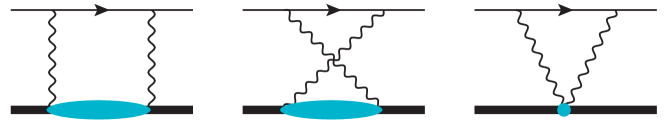
Figure 4: Two-photon exchange direct, crossed, and seagull diagrams.

We take into account only the relativistic corrections to the electric dipole polarizability contributions, $\delta^{(0)}_{D1}$, which represents the leading contribution $\delta^{(0)}_{\rm NR}$ in the non-relativistic $\eta$-expansion. Since $\delta^{(1)}_{\rm NR}$ and $\delta^{(2)}_{\rm NR}$ are already small, relativistic corrections to these higher-order terms are thus neglected in our analysis. Based on [38], the evaluation of the polarizability contributions are given in the point-proton and the relativistic limits by

$$\delta_{\rm pol}^{\rm R}=-8\alpha^{2}\phi^{2}(0)\int^{\infty}_{0}dq\left[\,\mathcal{R}_{L}(q)+\mathcal{R}_{T}(q)+\mathcal{R}_{S}(q)\,\right]{,}$$ (3degmabbhbtde)

where $q$ denotes the photon-exchange transfer momentum, and $\mathcal{R}_{L}$ and $\mathcal{R}_{T}$ are related respectively to the longitudinal and transverse photon polarization. $\mathcal{R}_{S}$, the seagull term, is required by gauge invariance and cancels exactly the singularity at $q=0$ in $\mathcal{R}_{T}$. These kernel functions are given in [38] as

$$\mathcal{R}_{L}(q) = \int^{\infty}_{0}d\omega S_{L}(\omega,\bm{q})g(\omega,q){,}$$ (3degmabbhbtdfa)

$$\mathcal{R}_{T}(q) = \int^{\infty}_{0}d\omega S_{T}(\omega,\bm{q})\left[-\frac{1}{4m_{r}q}\frac{\omega+2q}{(\omega+q)^{2}}+\frac{q^{2}}{4m_{r}^{2}}g(\omega,q)\right]{,}$$ (3degmabbhbtdfb)

$$\mathcal{R}_{S}(q) = \int^{\infty}_{0}d\omega S_{T}(\omega,0)\frac{1}{4m_{r}\omega}\left[\frac{1}{q}-\frac{1}{E_{q}}\right]\,,$$ (3degmabbhbtdfc)

with $E_{q}=\sqrt{q^{2}+m_{r}^{2}}$ and

$$g(\omega,q)=\frac{1}{2E_{q}}\left[\frac{1}{(E_{q}-m_{r})(E_{q}-m_{r}+\omega)}-\frac{1}{(E_{q}+m_{r})(E_{q}+m_{r}+\omega)}\right]{.}$$ (3degmabbhbtdfdg)

In the equations above, although we have taken the infinite-nuclear-mass approximation, the muon mass $m_{\mu}$ is replaced by the non-relativistic reduced mass $m_{r}$. By doing so, the leading term in the $\omega_{N}/m_{r}$-expansion of $\delta_{\rm pol}^{\rm R}$ in Eq. (3degmabbhbtde) matches exactly to $\delta^{(0)}_{D1}$ in Eq. (3degmabbd), and is thus subtracted out to avoid double counting. The remaining contributions represent the relativistic corrections to $\delta^{(0)}_{\rm NR}$. This approximation naturally takes into account the dominant relativistic recoil effects; while higher-order recoil corrections only enter at higher orders in the $m_{\mu}/M_{A}$ expansion and are neglected in this paper.

$S_{L}$ and $S_{T}$ are respectively the longitudinal and transverse response functions, which are defined as [38]

$$S_{L,T}(\omega,\bm{q})=\operatorname*{\mathchoice{\ooalign{$\displaystyle\sum$\cr$\displaystyle\int$\cr}}{\ooalign{\raisebox{0.14pt}{\scalebox{0.7}{$\textstyle\sum$}}\cr$\textstyle\int$\cr}}{\ooalign{\raisebox{0.2pt}{\scalebox{0.6}{$\scriptstyle\sum$}}\cr$\scriptstyle\int$\cr}}{\ooalign{\raisebox{0.2pt}{\scalebox{0.6}{$\scriptstyle\sum$}}\cr$\scriptstyle\int$\cr}}}\limits_{N\neq N_{0},J}|\langle NJ|\hat{O}_{L,T}(\bm{q})|N_{0}J_{0}\rangle|^{2}\delta(\omega-\omega_{N}){,}$$ (3degmabbhbtdfdh)

where $\hat{O}_{L}(\bm{q})=\hat{\mathcal{J}}_{0}(\bm{q})$ denotes the charge operator, and $\hat{O}_{T}(\bm{q})=\hat{q}\times\hat{\bm{\mathcal{J}}}(\bm{q})$ indicates the transverse part of the current operator. By defining the longitudinal direction $\bm{e}_{0}$ along $\bm{q}$, and two circular transverse directions $\bm{e}_{\pm 1}$, we have $\hat{O}_{T}(\bm{q})=\sum_{\lambda=\pm 1}\lambda(\bm{e}^{\dagger}_{\lambda}\cdot\hat{\bm{\mathcal{J}}})\bm{e}_{-\lambda}$, which leads to

$$S_{T}(\omega,\bm{q})=\operatorname*{\mathchoice{\ooalign{$\displaystyle\sum$\cr$\displaystyle\int$\cr}}{\ooalign{\raisebox{0.14pt}{\scalebox{0.7}{$\textstyle\sum$}}\cr$\textstyle\int$\cr}}{\ooalign{\raisebox{0.2pt}{\scalebox{0.6}{$\scriptstyle\sum$}}\cr$\scriptstyle\int$\cr}}{\ooalign{\raisebox{0.2pt}{\scalebox{0.6}{$\scriptstyle\sum$}}\cr$\scriptstyle\int$\cr}}}\limits_{N\neq N_{0},J}\sum_{\lambda=\pm 1}|\langle N,J|\bm{e}^{\dagger}_{\lambda}\cdot\hat{\bm{\mathcal{J}}}(\bm{q})|N_{0},J_{0}\rangle|^{2}\delta(\omega-\omega_{N}){.}$$ (3degmabbhbtdfdi)

We then express $\hat{\mathcal{J}}_{0}(\bm{q})$ and $\bm{e}^{\dagger}_{\lambda}\cdot\hat{\bm{\mathcal{J}}}(\bm{q})$ in the plane-wave expansion as [40]

$$\hat{\mathcal{J}}_{0}(\bm{q})=\sum\limits_{l\geq 0}\sqrt{4\pi(2l+1)}\,i^{l}C_{l}(q){,}$$ (3degmabbhbtdfdja)

$$\bm{e}^{\dagger}_{\lambda}\cdot\hat{\bm{\mathcal{J}}}(\bm{q})=-\sum_{l\geq 1}\sqrt{2\pi(2l+1)}i^{l}\left[\hat{T}^{\rm el}_{l-\lambda}(q)+\lambda\hat{T}^{\rm mag}_{l-\lambda}(q)\right]{,}$$ (3degmabbhbtdfdjb)

where $C_{l}(q)$, $\hat{T}^{\rm el}_{l\lambda}$ and $\hat{T}^{\rm mag}_{l\lambda}$ denote respectively the $l$th moments of the electric-charge, electric-transverse-current, and magnetic-transverse-current operators. Since the nucleus is much heavier than the muon, these moments are approximated for small $q$ by

$$C_{l}(q) =\frac{q^{l}}{(2l+1)!!}\int d^{3}x\,\hat{\mathcal{J}}_{0}(\bm{x})x^{l}Y_{l0}(\hat{x}){,}$$ (3degmabbhbtdfdjdka)

$$\hat{T}^{\rm el}_{l\lambda}(q) =\frac{-iq^{l-1}}{(2l+1)!!}\sqrt{\frac{l+1}{l}}\int d^{3}x\left\{\bm{\nabla}\cdot\hat{\bm{\mathcal{J}}_{c}}\,x^{l}Y_{l\lambda}+\frac{q^{2}}{l+1}\hat{\bm{\mathcal{J}}_{s}}\cdot\left[\bm{x}\times\bm{\nabla}x^{l}Y_{l\lambda}\right]\right\}{,}$$ (3degmabbhbtdfdjdkb)

$$\hat{T}^{\rm mag}_{l\lambda}(q) =\frac{iq^{l}}{(2l+1)!!}\sqrt{\frac{l+1}{l}}\int d^{3}x\left[\hat{\bm{\mathcal{J}}_{s}}+\frac{1}{l+1}\bm{x}\times\hat{\bm{\mathcal{J}}_{c}}\right]\cdot\bm{\nabla}x^{l}Y_{l\lambda}{,}$$ (3degmabbhbtdfdjdkc)

where $\hat{\bm{\mathcal{J}}}_{c}$ denotes the electric-convection current and $\hat{\bm{\mathcal{J}}_{s}}$ is the magnetic-spin current.

In the following, we separate the response functions into electric longitudinal, electric transverse and magnetic transverse parts, i.e., $\delta_{\rm pol}^{\rm R}=\delta_{L}^{(0)}+\delta_{T}^{(0)}+\delta_{M}^{(0)}$, and study their contributions respectively.

2.4.1 Electric longitudinal polarizability corrections

In the point-nucleon approximation, $\hat{\mathcal{J}}_{0}(\bm{x})=Z\hat{\rho}^{p}(\bm{x})=\sum_{a}^{Z}\delta^{(3)}(\bm{x}-\bm{R}_{a})$, so we have

$$C_{l}(q)=\frac{q^{l}}{(2l+1)!!}\sum_{a}^{Z}\bm{R}_{a}^{l}Y_{l0}(\hat{\bm{R}}_{a}){.}$$ (3degmabbhbtdfdjdkdl)

Since $C_{0}(q)=Z/\sqrt{4\pi}$ is constant, it does not contribute to the transition matrix element in Eq. (3degmabbhbtdfdh). Therefore, the leading term contributing to the longitudinal polarizability effect is from $C_{1}(q)$. It is related to the $z$-component of the electric-dipole operator by $C_{1}(q)=(Zq/3)\hat{D}_{1z}$. In this approximation, $\hat{\mathcal{J}}_{0}(\bm{q})\approx iZq\sqrt{4\pi/3}\hat{D}_{1z}$. By substituting $\hat{\mathcal{J}}_{0}(\bm{q})$’s low-momentum expression into Eq. (3degmabbhbtdfdh), we obtain the approximated electric longitudinal response function, which is related to the electric dipole response function by:

$$S_{L}^{(0)}(\omega,\bm{q}) = \frac{4\pi}{3}Z^{2}q^{2}\operatorname*{\mathchoice{\ooalign{$\displaystyle\sum$\cr$\displaystyle\int$\cr}}{\ooalign{\raisebox{0.14pt}{\scalebox{0.7}{$\textstyle\sum$}}\cr$\textstyle\int$\cr}}{\ooalign{\raisebox{0.2pt}{\scalebox{0.6}{$\scriptstyle\sum$}}\cr$\scriptstyle\int$\cr}}{\ooalign{\raisebox{0.2pt}{\scalebox{0.6}{$\scriptstyle\sum$}}\cr$\scriptstyle\int$\cr}}}\limits_{N\neq N_{0},J}|\langle NJ|\hat{D}_{1z}|N_{0}J_{0}\rangle|^{2}\delta(\omega-\omega_{N})$$ (3degmabbhbtdfdjdkdu)

$$= \frac{4\pi}{9}Z^{2}q^{2}S_{D_{1}}(\omega){,}$$ (3degmabbhbtdfdjdkdv)

where $|\langle NJ|\hat{D}_{1z}|N_{0}J_{0}\rangle|^{2}=\frac{1}{3(2J_{0}+1)}|\langle NJ||\hat{D}_{1}||N_{0}J_{0}\rangle|^{2}$ is used by averaging the full photon angle, which is arbitrary to the direction of the nuclear quantization [40].

We substitute Eq. (3degmabbhbtdfdjdkdu) into Eqs. (3degmabbhbtde) and (3degmabbhbtdfa), and obtain the electric longitudinal polarizability contribution as

$$\delta_{L}^{(0)}=\frac{32\pi}{9}(Z\alpha)^{2}\phi^{2}(0)\int^{\infty}_{0}d\omega\,S_{D_{1}}(\omega)\,\mathcal{F}_{L}(\omega/m_{r}){,}$$ (3degmabbhbtdfdjdkdw)

where $\mathcal{F}_{L}$ represents a $q$-integration, i.e., $\mathcal{F}_{L}(\omega/m_{r})\equiv-\int^{\infty}_{0}dq\,q^{2}g(\omega,q)$, whose evaluation yields

$$\mathcal{F}_{L}(\lambda)=\sqrt{\frac{\lambda-2}{\lambda}}\operatorname{arctanh}\sqrt{\frac{\lambda-2}{\lambda}}-\sqrt{\frac{\lambda+2}{\lambda}}\operatorname{arctanh}\sqrt{\frac{\lambda}{\lambda+2}}{,}$$ (3degmabbhbtdfdjdkdx)

where $\lambda=\omega/m_{r}$. We note that $\mathcal{F}_{L}$ is real for $\lambda>0$ when analytic continuation at $\lambda=2$ is applied.

Eq. (3degmabbhbtdfdjdkdw) contains relativistic corrections to only the electric dipole polarizability contribution; while relativistic corrections to higher-multipole contributions are neglected in the low-$q$ approximation made in Eq. (3degmabbhbtdfdjdkdu). If we expand $\mathcal{F}_{L}$ for small $\lambda=\omega/m_{r}$, the leading and sub-leading terms are

$$\mathcal{F}_{L}(\omega/m_{r}\rightarrow 0)\approx-\frac{\pi}{2}\sqrt{\frac{2m_{r}}{\omega}}\left(1-\frac{\omega}{4m_{r}}\right)+\cdots$$ (3degmabbhbtdfdjdkdy)

The first term in $\mathcal{F}_{L}$ matches exactly to $\delta^{(0)}_{D1}$ in Eq. (3degmabbd). Therefore, we subtract the leading term to avoid double counting. We then obtain the relativistic longitudinal polarizability correction as

$$\delta_{L}^{(0)}=\frac{32\pi}{9}(Z\alpha)^{2}\phi^{2}(0)\int^{\infty}_{0}d\omega\,S_{D_{1}}(\omega)\left[\mathcal{F}_{L}\left(\frac{\omega}{m_{r}}\right)+\frac{\pi}{2}\sqrt{\frac{2m_{r}}{\omega}}\right]{.}$$ (3degmabbhbtdfdjdkdz)

One can use dimensional analysis on the sub-leading term in $\mathcal{F}_{L}$ to roughly estimate the size of $\delta_{L}^{(0)}$. The typical scale of $\omega$ is represented by the first nuclear excitation energy $\omega_{\rm th}$. Therefore, $\delta_{L}^{(0)}$ is approximately smaller than $\delta_{D1}^{(0)}$ by order $\omega_{\rm th}/m_{\mu}$.

2.4.2 Electric transverse polarizability corrections

In the $q\rightarrow 0$ limit, the electric transverse current is dominated by its first moment, which is related to the electric-dipole operator by

$$\hat{T}^{\rm el}_{1\lambda}(q\rightarrow 0)=-i\frac{\sqrt{2}}{3}\int d^{3}x\bm{\nabla}\cdot\hat{\bm{\mathcal{J}}}_{c}\,xY_{1\lambda}(\hat{x})=\frac{\sqrt{2}}{3}Z\omega\hat{D}_{1\lambda}{,}$$ (3degmabbhbtdfdjdkea)

where the Siegert’s theorem $\bm{\nabla}\cdot\hat{\bm{\mathcal{J}}}_{c}=i\omega\mathcal{J}_{0}$ is used. This leads to the dominant component of the electric transverse current in low-$q$ expansion as $\bm{e}^{\dagger}_{\lambda}\cdot\hat{\bm{\mathcal{J}}}^{\rm el}\approx-i\sqrt{4\pi/3}\,Z\omega\,\hat{D}_{1-\lambda}$. By substituting the low-$q$ approximation of $\bm{e}^{\dagger}_{\lambda}\cdot\hat{\bm{\mathcal{J}}}^{\rm el}$ into Eq. (3degmabbhbtdfdi), we obtain the dominant component of the electric transverse response function as

$$S_{T}^{{\rm el}\,(0)}(\omega,\bm{q}) = \frac{4\pi}{3}Z^{2}\omega^{2}\operatorname*{\mathchoice{\ooalign{$\displaystyle\sum$\cr$\displaystyle\int$\cr}}{\ooalign{\raisebox{0.14pt}{\scalebox{0.7}{$\textstyle\sum$}}\cr$\textstyle\int$\cr}}{\ooalign{\raisebox{0.2pt}{\scalebox{0.6}{$\scriptstyle\sum$}}\cr$\scriptstyle\int$\cr}}{\ooalign{\raisebox{0.2pt}{\scalebox{0.6}{$\scriptstyle\sum$}}\cr$\scriptstyle\int$\cr}}}\limits_{N\neq N_{0},J}\sum_{\lambda=\pm 1}|\langle NJ|\hat{D}_{1\lambda}|N_{0}J_{0}\rangle|^{2}\delta(\omega-\omega_{N})$$ (3degmabbhbtdfdjdkej)

$$= \frac{8\pi}{9}Z^{2}\omega^{2}S_{D_{1}}(\omega){,}$$ (3degmabbhbtdfdjdkek)

where $\sum_{\lambda=\pm 1}|\langle NJ|\hat{D}_{1\lambda}|N_{0}J_{0}\rangle|^{2}=\frac{2}{3(2J_{0}+1)}|\langle NJ||\hat{D}_{1}||N_{0}J_{0}\rangle|^{2}$ after averaging the photon angle. By substituting Eq. (3degmabbhbtdfdjdkej) into Eqs. (3degmabbhbtde), (3degmabbhbtdfb) and (3degmabbhbtdfc), we obtain the relativistic electric transverse polarizability correction as

$$\delta_{T}^{(0)} = -8\alpha^{2}\phi^{2}(0)\int^{\infty}_{0}dq\left[\mathcal{R}_{T}+\mathcal{R}_{S}\right]^{\rm el}$$ (3degmabbhbtdfdjdkel)

$$= \frac{16\pi}{9}(Z\alpha)^{2}\phi^{2}(0)\int^{\infty}_{0}d\omega\,S_{D_{1}}(\omega)\mathcal{F}_{T}(\omega/m_{r}){,}$$

where $\mathcal{R}_{S}^{el}$ cancels the infrared divergence in $\mathcal{R}_{T}^{el}$ at $q=0$. $\mathcal{F}_{T}$ represents a $q$-integration:

$$\mathcal{F}_{T}\left(\frac{\omega}{m_{r}}\right)=-4\omega^{2}\int^{\infty}_{0}dq\left\{-\frac{1}{4m_{r}q}\frac{\omega+2q}{(\omega+q)^{2}}+\frac{q^{2}}{4m_{r}^{2}}g(\omega,q)+\frac{1}{4m_{r}\omega}\left[\frac{1}{q}-\frac{1}{E_{q}}\right]\right\}{.}$$ (3degmabbhbtdfdjdkem)

The evaluation of the integration above yields

$$\mathcal{F}_{T}(\lambda)=\lambda+\lambda\ln(2\lambda)+\lambda^{2}\mathcal{F}_{L}(\lambda){.}$$ (3degmabbhbtdfdjdken)

We roughly estimate the size of $\delta_{T}^{(0)}$ by taking the dominant term of $\mathcal{F}_{T}$ in the small-$\omega/m_{r}$ expansion, i.e., $\mathcal{F}_{T}\approx(\omega/m_{r})\ln(2\omega/m_{r})$. Comparing the energy weights in Eq. (3degmabbd) and (3degmabbhbtdfdjdkel), the contribution of $\delta_{T}^{(0)}$ is approximately smaller than $\delta_{L}^{(0)}$ by order $\sqrt{\omega_{\rm th}/m_{\mu}}\ln(\omega_{\rm th}/m_{\mu})$.

2.4.3 Magnetic transverse polarizability corrections

In the limit $q\rightarrow 0$, $\hat{T}^{\rm mag}_{1\lambda}$ plays the dominant role in the magnetic transverse current. In the point-nucleon limit, we express $\hat{\bm{\mathcal{J}}_{s}}$ and $\bm{x}\times\hat{\bm{\mathcal{J}}_{c}}$ respectively as

$$\hat{\bm{\mathcal{J}}_{s}}(\bm{x}) = \frac{1}{2m_{p}}\sum_{i}^{A}(g_{p}\hat{e}_{p,i}+g_{n}\hat{e}_{n,i})\bm{s}_{i}\,\delta^{(3)}\left(\bm{x}-\bm{R}_{i}\right){,}$$ (3degmabbhbtdfdjdkeoa)

$$\bm{x}\times\hat{\bm{\mathcal{J}}_{c}}(\bm{x}) = \frac{1}{m_{p}}\sum_{i}^{Z}\bm{l}_{i}\hat{e}_{p,i}\,\delta^{(3)}(\bm{x}-\bm{R}_{i}){,}$$ (3degmabbhbtdfdjdkeob)

where $g_{p}=5.586$ and $g_{n}=-3.826$. $\bm{s}_{i}$ and $\bm{l}_{i}$ indicate the spin and angular momentum of the $i$th nucleon. Using these equations above, we obtain that $\hat{T}^{\rm mag}_{1\lambda}=iZq\hat{M}_{1\lambda}/(2m_{p}\sqrt{6\pi})$ [40], with $\hat{M}_{1}$ denoting a magnetic-dipole operator:

$$\hat{M}_{1}\equiv\frac{1}{Z}\sum_{i}^{A}\left[(g_{p}\hat{e}_{p,i}+g_{n}\hat{e}_{n,i})\bm{s}_{i}+\hat{e}_{p,i}\bm{l}_{i}\right]{.}$$ (3degmabbhbtdfdjdkeoep)

In the low-$q$ limit, the magnetic current operator is dominated by the magnetic-dipole part, i.e., $[\bm{e}^{\dagger}_{\lambda}\cdot\hat{\bm{\mathcal{J}}}]_{\rm mag}\approx\lambda Zq\hat{M}_{1-\lambda}/(2m_{p})$, and the magnetic transverse response function is approximated by

$$S_{T}^{{\rm mag}\,(0)}(\omega,\bm{q})=\frac{Z^{2}q^{2}}{6m_{p}^{2}}S_{M_{1}}(\omega){,}$$ (3degmabbhbtdfdjdkeoeq)

where $S_{M_{1}}$ is the magnetic-dipole structure function

$$S_{M_{1}}(\omega)=\frac{1}{2J_{0}+1}\operatorname*{\mathchoice{\ooalign{$\displaystyle\sum$\cr$\displaystyle\int$\cr}}{\ooalign{\raisebox{0.14pt}{\scalebox{0.7}{$\textstyle\sum$}}\cr$\textstyle\int$\cr}}{\ooalign{\raisebox{0.2pt}{\scalebox{0.6}{$\scriptstyle\sum$}}\cr$\scriptstyle\int$\cr}}{\ooalign{\raisebox{0.2pt}{\scalebox{0.6}{$\scriptstyle\sum$}}\cr$\scriptstyle\int$\cr}}}\limits_{N\neq N_{0},J}|\langle NJ||\hat{M}_{1}||N_{0}J_{0}\rangle|^{2}\delta(\omega-\omega_{N}){.}$$ (3degmabbhbtdfdjdkeoer)

Combining Eqs. (3degmabbhbtdfdjdkeoeq), (3degmabbhbtde) and (3degmabbhbtdfb), we obtain the magnetic transverse polarizability contribution:

$$\delta_{M}^{(0)} = -8\alpha^{2}\phi^{2}(0)\int^{\infty}_{0}dq\,\mathcal{R}_{T}^{\rm mag}$$ (3degmabbhbtdfdjdkeoes)

$$= \frac{(Z\alpha)^{2}}{3m_{p}^{2}}\phi^{2}(0)\int^{\infty}_{0}d\omega\,S_{M_{1}}(\omega)\mathcal{F}_{M}(\omega/m_{r}){,}$$

A seagull term $\mathcal{R}_{S}^{\rm mag}$ is not needed in Eq. (3degmabbhbtdfdjdkeoes), since $R_{T}^{\rm mag}$ is finite at $q=0$. $\mathcal{F}_{M}$ defines a $q$-integration:

$$\mathcal{F}_{M}\left(\frac{\omega}{m_{r}}\right)=-4\int^{\infty}_{0}dq\,q^{2}\left[-\frac{1}{4m_{r}q}\frac{\omega+2q}{(\omega+q)^{2}}+\frac{q^{2}}{4m_{r}^{2}}g(\omega,q)\right]{,}$$ (3degmabbhbtdfdjdkeoet)

whose evaluation yields

$$\mathcal{F}_{M}(\lambda)=\sqrt{\lambda}\left[(\lambda-2)^{\frac{3}{2}}\operatorname{arctanh}\sqrt{\frac{\lambda-2}{\lambda}}-(\lambda+2)^{\frac{3}{2}}\operatorname{arctanh}\sqrt{\frac{\lambda}{\lambda+2}}\right]+\lambda+3\lambda\ln(2\lambda){.}$$ (3degmabbhbtdfdjdkeoeu)

Similarly, $\mathcal{F}_{M}$ is real for $\lambda>0$ when analytic continuation is applied at $\lambda=2$. When $\lambda=\omega/m_{r}\ll 1$, $\mathcal{F}_{M}\approx\pi\sqrt{2\omega/m_{r}}$, which is an approximated energy-weight used in our previous estimates of the magnetic-dipole polarizability contribution [32, 41]. In this paper, we use the complete expression (3degmabbhbtdfdjdkeoeu) as a more accurate energy-weight for the magnetic-dipole sum rule. Different from $\delta_{L,T}^{(0)}$, the magnetic-dipole sum rule is characterized by a different threshold energy, because the magnetic excitation in light nuclei normally involves higher lying states than does the electric-dipole excitation. Suppressed by the $1/m_{p}^{2}$ factor, we expect $\delta_{M}^{(0)}$ to be much smaller than $\delta^{(0)}_{D1}$.

2.5 Nucleon-size corrections

When considering the intrinsic charge distribution of nucleons, the position of proton in Eq. (3degmn) needs to be replaced by a convolution over the proton and neutron charge densities. Therefore, Eq. (3degmn) is modified by

$$\eqalign{\Delta H=\sum_{a}^{A}\Delta V_{a}(\bm{r},\bm{R}_{a}){,}\\ \Delta V_{a}(\bm{r},\bm{R}_{a})=\Delta V_{p}(\bm{r},\bm{R}_{a})\hat{e}_{p,a}+\Delta V_{n}(\bm{r},\bm{R}_{a})\hat{e}_{n,a}{,}}$$ (3degmabbhbtdfdjdkeoev)

where $\Delta V_{p}$ and $\Delta V_{n}$ are defined respectively as

$$\Delta V_{p}(\bm{r},\bm{R}_{a}) \equiv \alpha\left(\frac{1}{r}-\int d^{3}R^{\prime}\,\frac{n_{p}(\bm{R}^{\prime}-\bm{R}_{a})}{|\bm{r}-\bm{R}^{\prime}|}\right){,}$$ (3degmabbhbtdfdjdkeoewa)

$$\Delta V_{n}(\bm{r},\bm{R}_{a}) \equiv -\alpha\int d^{3}R^{\prime}\,\frac{n_{n}(\bm{R}^{\prime}-\bm{R}_{a})}{|\bm{r}-\bm{R}^{\prime}|}{,}$$ (3degmabbhbtdfdjdkeoewb)

with $n_{p}$ and $n_{n}$ indicating the intrinsic proton and neutron charge densities.

Besides $\rho^{p}_{N}$ in Eq. (3degmaa), we also define at this point the point-neutron transition density function

$$\rho^{n}_{N}(\bm{R}) = \langle N|\frac{1}{Z}\sum_{a}^{A}\delta(\bm{R}-\bm{R}_{a})\hat{e}_{n,a}|N_{0}\rangle{,}$$ (3degmabbhbtdfdjdkeoewex)

with $\rho^{n}_{0}(\bm{R})$ denoting the point-neutron densities defined in Eq. (3dega). Using this function we write

$$\sum_{a}^{A}\langle N|\Delta V_{a}(\bm{r},\bm{R}_{a})|N_{0}\rangle = Z\int d^{3}R\left[\rho^{p}_{N}(\bm{R})\Delta V_{p}(\bm{r},\bm{R})+\rho^{n}_{N}(\bm{R})\Delta V_{n}(\bm{r},\bm{R})\right]{.}$$ (3degmabbhbtdfdjdkeoewey)

$\delta_{\rm pol}^{A}$ is then expressed as

$$\delta_{\rm pol}^{A}=\sum_{c,c^{\prime}=n,p}\operatorname*{\mathchoice{\ooalign{$\displaystyle\sum$\cr$\displaystyle\int$\cr}}{\ooalign{\raisebox{0.14pt}{\scalebox{0.7}{$\textstyle\sum$}}\cr$\textstyle\int$\cr}}{\ooalign{\raisebox{0.2pt}{\scalebox{0.6}{$\scriptstyle\sum$}}\cr$\scriptstyle\int$\cr}}{\ooalign{\raisebox{0.2pt}{\scalebox{0.6}{$\scriptstyle\sum$}}\cr$\scriptstyle\int$\cr}}}_{N\neq N_{0}}\int d^{3}Rd^{3}R^{\prime}\rho_{N}^{c*}(\bm{R}){W}^{cc^{\prime}}(\bm{R},\bm{R}^{\prime},\omega_{N})\rho^{c^{\prime}}_{N}(\bm{R}^{\prime}){,}$$ (3degmabbhbtdfdjdkeoewez)

where the muon matrix elements ${W}^{cc^{\prime}}$ (with $c,c^{\prime}=n,p$) are defined as

$${W}^{cc^{\prime}}(\bm{R},\bm{R}^{\prime},\omega_{N}) = -Z^{2}\phi^{2}(0)\int d^{3}rd^{3}r^{\prime}\Delta V_{c}(\bm{r},\bm{R})\langle\bm{r}|\frac{1}{\frac{q^{2}}{2m_{r}}+\omega_{N}}|\bm{r}^{\prime}\rangle\Delta V_{c^{\prime}}(\bm{r}^{\prime},\bm{R}^{\prime}){.}$$ (3degmabbhbtdfdjdkeoewfa)

Now we use the Fourier transform of $\Delta V_{p}(\bm{r},\bm{R})$ and $\Delta V_{n}(\bm{r},\bm{R})$ with respect to the muon-coordinates and have

$$\Delta\tilde{V}_{p}(\bm{q},\bm{R}) = \int d^{3}rV_{p}(\bm{r},\bm{R})e^{i\bm{q}\cdot\bm{r}}=\frac{4\pi\alpha}{q^{2}}\left(1-\tilde{n}_{p}(q)e^{i\bm{q}\cdot\bm{R}}\right){,}$$ (3degmabbhbtdfdjdkeoewfb)

$$\Delta\tilde{V}_{n}(\bm{q},\bm{R}) = \int d^{3}rV_{n}(\bm{r},\bm{R})e^{i\bm{q}\cdot\bm{r}}=-\frac{4\pi\alpha}{q^{2}}\tilde{n}_{n}(q)e^{i\bm{q}\cdot\bm{R}}{,}$$ (3degmabbhbtdfdjdkeoewfc)

where $\tilde{n}_{p/n}(q)=\int d^{3}R\,n_{p/n}(\bm{R})e^{i\bm{q}\cdot\bm{R}}$ is the Fourier transform of the nucleon charge density, which depends only on $q=|\bm{q}|$. In the non-relativistic limit, $\tilde{n}_{p}(q)$ and $\tilde{n}_{n}(q)$ represent the nucleon electric form factors, with $\tilde{n}_{p}(0)=1$ and $\tilde{n}_{n}(0)=0$ at $q=0$. Inserting the above expressions into Eq. (3degmabbhbtdfdjdkeoewfa), we have

$${W}^{pp} = -Z^{2}\phi^{2}(0)\int\frac{d^{3}q}{(2\pi)^{3}}\left(\frac{4\pi\alpha}{q^{2}}\right)^{2}\frac{1}{\frac{q^{2}}{2m_{r}}+\omega_{N}}\left[\tilde{n}_{p}^{2}(q)e^{i\bm{q}\cdot(\bm{R}-\bm{R}^{\prime})}-1\right]{,}$$ (3degmabbhbtdfdjdkeoewfda)

$${W}^{np/pn} = -Z^{2}\phi^{2}(0)\int\frac{d^{3}q}{(2\pi)^{3}}\left(\frac{4\pi\alpha}{q^{2}}\right)^{2}\frac{1}{\frac{q^{2}}{2m_{r}}+\omega_{N}}\tilde{n}_{p}(q)\tilde{n}_{n}(q)e^{i\bm{q}\cdot(\bm{R}-\bm{R}^{\prime})}{,}$$ (3degmabbhbtdfdjdkeoewfdb)

$${W}^{nn} = -Z^{2}\phi^{2}(0)\int\frac{d^{3}q}{(2\pi)^{3}}\left(\frac{4\pi\alpha}{q^{2}}\right)^{2}\frac{1}{\frac{q^{2}}{2m_{r}}+\omega_{N}}\tilde{n}_{n}^{2}(q)e^{i\bm{q}\cdot(\bm{R}-\bm{R}^{\prime})}{.}$$ (3degmabbhbtdfdjdkeoewfdc)

Similarly to Eq. (3degmabam), here we have omitted terms that depend on $R$ or $R^{\prime}$ alone. Such terms yield matrix elements proportional to $\langle N_{0}|R^{n}|N\rangle\langle N|N_{0}\rangle$, which are zero due to the orthogonality between nuclear states $|N_{0}\rangle$ and $|N\rangle$.

For convenience of calculations, we take low-$q$ approximation of $\tilde{n}_{p}(q)$ and $\tilde{n}_{n}(q)$, and expand them up to $q^{2}$:

$$\tilde{n}_{p}(q) = \frac{1}{(1+q^{2}/\beta^{2})^{2}}\approx 1-2q^{2}/\beta^{2}+\cdots{,}$$ (3degmabbhbtdfdjdkeoewfdfea)

$$\tilde{n}_{n}(q) = \frac{\lambda q^{2}}{(1+q^{2}/\beta^{2})^{3}}\approx\lambda q^{2}+\cdots{,}$$ (3degmabbhbtdfdjdkeoewfdfeb)

where $\beta=\sqrt{12/r_{p}^{2}}$ and $\lambda=-r_{n}^{2}/6$ are parameterized by the proton and neutron charge radius squared. We take $r_{p}=0.8409\;{\rm fm}$ from the $\mu$H measurement, and $r_{n}^{2}=-0.1161\;{\rm fm}^{2}$ from Particle Data Group [42], and obtain $\beta=4.120\;{\rm fm}^{-1}$ and $\lambda=0.01935\;{\rm fm}^{2}$. Therefore, $\tilde{n}_{c}(q)\tilde{n}_{c^{\prime}}(q)$ is expanded up to $q^{2}$ as

$$\tilde{n}_{p}^{2}(q)\approx 1-4q^{2}/\beta^{2}{,}$$ (3degmabbhbtdfdjdkeoewfdfeffa)

$$\tilde{n}_{n}(q)\tilde{n}_{p}(q)\approx\lambda q^{2}{,}$$ (3degmabbhbtdfdjdkeoewfdfeffb)

$$\tilde{n}_{n}^{2}(q)\approx 0{.}$$ (3degmabbhbtdfdjdkeoewfdfeffc)

The low-$q$ truncation leads to an approximated treatment of proton-proton correction and proton-neutron overlap contribution to $\delta_{\rm pol}^{A}$. As indicated by Eq. (3degmabbhbtdfdjdkeoewfdfeffc), the neutron-neutron contribution enters at one order higher and is thus omitted.

By inserting Eq. (3degmabbhbtdfdjdkeoewfdfeffa) into Eq. (3degmabbhbtdfdjdkeoewfda), we rewrite ${W}^{pp}$ as

$${W}^{pp} \approx -Z^{2}\phi^{2}(0)\left[1+\frac{2}{\beta^{2}}\nabla_{R}^{2}+\frac{2}{\beta^{2}}\nabla_{R^{\prime}}^{2}\right]\int\frac{d^{3}q}{(2\pi)^{3}}\left(\frac{4\pi\alpha}{q^{2}}\right)^{2}\frac{1}{\frac{q^{2}}{2m_{r}}+\omega_{N}}\left(e^{i\bm{q}\cdot(\bm{R}-\bm{R}^{\prime})}-1\right){.}$$ (3degmabbhbtdfdjdkeoewfdfefffg)

After integrating over the $q$ dependence in Eq. (3degmabbhbtdfdjdkeoewfdfefffg), the term $1$ in the leftmost square bracket of Eq. (3degmabbhbtdfdjdkeoewfdfefffg) yields exactly the point-nucleon result $\delta_{\rm pol}^{\rm NR}$ as indicated by Eq. (3degmabam). By dropping the “1” term, the remaining expression in Eq. (3degmabbhbtdfdjdkeoewfdfefffg) results in the proton-proton correction $\Delta{W}^{pp}$. Utilizing the $\eta=\sqrt{2m_{r}\omega_{N}}|\bm{R}-\bm{R}^{\prime}|$ expansion up to the fourth order, we have

$$\Delta{W}^{pp} = \frac{4\pi}{3\beta^{2}}(Z\alpha)^{2}\phi^{2}(0)\sqrt{\frac{2m_{r}}{\omega_{N}}}(\nabla_{R}^{2}+\nabla_{R^{\prime}}^{2})$$

$$\times\left\{|\bm{R}-\bm{R}^{\prime}|^{2}-\frac{1}{4}\sqrt{2m_{r}\omega_{N}}|\bm{R}-\bm{R}^{\prime}|^{3}+\frac{1}{10}m_{r}\omega_{N}|\bm{R}-\bm{R}^{\prime}|^{4}\right]$$

$$= \frac{8\pi}{3\beta^{2}}(Z\alpha)^{2}\phi^{2}(0)\sqrt{\frac{2m_{r}}{\omega_{N}}}\left[6-3\sqrt{2m_{r}\omega_{N}}|\bm{R}-\bm{R}^{\prime}|+2m_{r}\omega_{N}|\bm{R}-\bm{R}^{\prime}|^{2}\right]{.}$$ (3degmabbhbtdfdjdkeoewfdfefffj)

The first term in the bracket does not contribute to the nuclear polarizability, since it does not depend on $\bm{R}$ and $\bm{R}^{\prime}$, Consequently the leading proton-size correction to $\delta_{\rm pol}^{A}$ is

$$\delta^{(1)}_{pp}=\ -\frac{16\pi m_{r}}{\beta^{2}}(Z\alpha)^{2}\phi^{2}(0)\int\int d^{3}Rd^{3}R^{\prime}|\bm{R}-\bm{R}^{\prime}|\,\left(\rho_{0}^{pp}(\bm{R},\bm{R}^{\prime})-\rho_{0}^{p}(\bm{R})\rho_{0}^{p}(\bm{R}^{\prime})\right){.}$$ (3degmabbhbtdfdjdkeoewfdfefffk)

Similarly, the sub-leading proton-proton correction is analyzed from the last term in Eq. (2.5), which yields

$$\delta^{(2)}_{pp}=-\frac{256\pi^{2}m_{r}^{2}}{9\beta^{2}}(Z\alpha)^{2}\phi^{2}(0)\int^{\infty}_{0}d\omega\,\sqrt{\frac{\omega}{2m_{r}}}S_{D_{1}}(\omega){.}$$ (3degmabbhbtdfdjdkeoewfdfefffl)

The neutron-proton overlap muonic matrix element $\Delta{W}^{np}$ is calculated in the $\eta$-expansion up to the fourth order:

$$\Delta{W}^{np} = {W}^{np}+{W}^{pn}$$ (3degmabbhbtdfdjdkeoewfdfefffm)

$$= -\frac{2\lambda\pi}{3}(Z\alpha)^{2}\phi^{2}(0)\sqrt{\frac{2m_{r}}{\omega_{N}}}(\nabla_{R}^{2}+\nabla_{R^{\prime}}^{2})$$

$$\times\left[|\bm{R}-\bm{R}^{\prime}|^{2}-\frac{1}{4}\sqrt{2m_{r}\omega_{N}}|\bm{R}-\bm{R}^{\prime}|^{3}+\frac{1}{10}m_{r}\omega_{N}|\bm{R}-\bm{R}^{\prime}|^{4}\right]$$

$$= -\frac{4\lambda\pi}{3}(Z\alpha)^{2}\phi^{2}(0)\sqrt{\frac{2m_{r}}{\omega_{N}}}\left[6-3\sqrt{2m_{r}\omega_{N}}|\bm{R}-\bm{R}^{\prime}|+2m_{r}\omega_{N}|\bm{R}-\bm{R}^{\prime}|^{2}\right]{.}$$

Similarly, we drop the constant term in the last bracket using orthogonality condition. Therefore, the leading neutron-proton overlap correction to $\delta_{\rm pol}^{A}$ is

$$\delta^{(1)}_{np}=8\lambda\pi m_{r}(Z\alpha)^{2}\phi^{2}(0)\int\int d^{3}Rd^{3}R^{\prime}|\bm{R}-\bm{R}^{\prime}|\,\left[\rho_{0}^{np}(\bm{R},\bm{R}^{\prime})-\rho_{0}^{n}(\bm{R})\rho_{0}^{p}(\bm{R}^{\prime})\right]{,}$$ (3degmabbhbtdfdjdkeoewfdfefffn)

where the neutron-proton two-body density $\rho_{0}^{np}$ is given in Eq. (3degb).

The sub-leading n-p overlap contribution is written as

$$\delta^{(2)}_{np}=\lambda\frac{128\pi^{2}m_{r}^{2}}{9}(Z\alpha)^{2}\phi^{2}(0)\int^{\infty}_{0}d\omega\,\sqrt{\frac{\omega}{2m_{r}}}S_{D_{1}}^{(np)}(\omega){,}$$ (3degmabbhbtdfdjdkeoewfdfefffo)

where $S_{D_{1}}^{(np)}$ denotes a neutron-proton overlapping dipole response function:

$$S_{D_{1}}^{(np)}(\omega)=\frac{1}{2J_{0}+1}{\rm Re}\operatorname*{\mathchoice{\ooalign{$\displaystyle\sum$\cr$\displaystyle\int$\cr}}{\ooalign{\raisebox{0.14pt}{\scalebox{0.7}{$\textstyle\sum$}}\cr$\textstyle\int$\cr}}{\ooalign{\raisebox{0.2pt}{\scalebox{0.6}{$\scriptstyle\sum$}}\cr$\scriptstyle\int$\cr}}{\ooalign{\raisebox{0.2pt}{\scalebox{0.6}{$\scriptstyle\sum$}}\cr$\scriptstyle\int$\cr}}}\limits_{N\neq N_{0},J}\langle N_{0}J_{0}||\hat{D}_{1}^{n\dagger}||NJ\rangle\langle NJ||\hat{D}_{1}^{p}||N_{0}J_{0}\rangle\delta(\omega-\omega_{N}){,}$$ (3degmabbhbtdfdjdkeoewfdfefffp)

with $D_{1}^{n/p}\equiv\frac{1}{Z}\sum_{a}^{A}R_{a}Y_{1}(\hat{R}_{a})\hat{e}_{n/p,a}$ defining the neutron/proton dipole operator.

For both $D_{1}^{n}$ and $D_{1}^{p}$, the iso-scalar part of both operators induces a nuclear center-of-mass motion and vanishes between the nuclear ground and excited states. The remaining iso-vector parts of both operators have an opposite sign, this yields the following condition

$$\langle N_{0}J_{0}||\hat{D}_{1}^{n}||NJ\rangle=-\langle N_{0}J_{0}||\hat{D}_{1}^{p}||NJ\rangle{.}$$ (3degmabbhbtdfdjdkeoewfdfefffq)

Therefore, we have $S_{D_{1}}^{(np)}=-S_{D_{1}}$, which holds for all nuclei. We then rewrite the sub-leading neutron-proton overlap contribution as

$$\delta^{(2)}_{np}=-\lambda\frac{128\pi^{2}m_{r}^{2}}{9}(Z\alpha)^{2}\phi^{2}(0)\int^{\infty}_{0}d\omega\,\sqrt{\frac{\omega}{2m_{r}}}S_{D_{1}}(\omega){.}$$ (3degmabbhbtdfdjdkeoewfdfefffr)

Combining Eqs. (3degmabbhbtdfdjdkeoewfdfefffk) and (3degmabbhbtdfdjdkeoewfdfefffn), we have the dominant nucleon-size correction, $\delta^{(1)}_{R1}+\delta^{(1)}_{Z1}$,

$$\delta^{(1)}_{R1} = -8\pi m_{r}(Z\alpha)^{2}\phi^{2}(0)\int\int d^{3}Rd^{3}R^{\prime}|\bm{R}-\bm{R}^{\prime}|\left[\frac{2}{\beta^{2}}\rho_{0}^{pp}(\bm{R},\bm{R}^{\prime})-\lambda\rho_{0}^{np}(\bm{R},\bm{R}^{\prime})\right]{,}$$ (3degmabbhbtdfdjdkeoewfdfefffsa)

$$\delta^{(1)}_{Z1} = 8\pi m_{r}(Z\alpha)^{2}\phi^{2}(0)\int\int d^{3}Rd^{3}R^{\prime}|\bm{R}-\bm{R}^{\prime}|\rho_{0}^{p}(\bm{R})\left[\frac{2}{\beta^{2}}\rho_{0}^{p}(\bm{R}^{\prime})-\lambda\rho_{0}^{n}(\bm{R}^{\prime})\right]{.}$$ (3degmabbhbtdfdjdkeoewfdfefffsb)

Adding $\delta^{(1)}_{Z1}$ in Eq. (3degmabbhbtdfdjdkeoewfdfefffsb) to $\delta^{(1)}_{Z3}$ in Eq. (3degmabbhb), we obtain the nuclear part of the elastic Zemach contribution as

$$\delta_{\rm Zem}^{A}=-\left[\delta^{(1)}_{Z3}+\delta^{(1)}_{Z1}\right]{.}$$ (3degmabbhbtdfdjdkeoewfdfefffsft)

The combination of Eqs. (3degmabbhbtdfdjdkeoewfdfefffl) and (3degmabbhbtdfdjdkeoewfdfefffr) gives the sub-dominant nucleon-size correction

$$\delta^{(2)}_{NS}=-\frac{128}{9}\pi^{2}m_{r}^{2}(Z\alpha)^{2}\phi^{2}(0)\left[\frac{2}{\beta^{2}}+\lambda\right]\int^{\infty}_{0}d\omega\sqrt{\frac{\omega}{2m_{r}}}S_{D_{1}}(\omega){.}$$ (3degmabbhbtdfdjdkeoewfdfefffsfu)

2.6 Intrinsic nucleon two-photon exchange

Besides the two-photon exchange contribution which probes the nuclear structures, the intrinsic nucleon TPE effects also make corrections to the muonic atom spectrum. When the muon exchanges two photons with a single nucleon at a short-time scale, it probes only the internal structure of a single proton (or neutron), which is independent of the nuclear wave function.

2.6.1 Nucleon elastic Zemach contribution

The inclusion of nucleon-size correction in Section 2.5 is based on a low-$q$ expansion of the proton (or neutron) electric form factors. In other words, the expansion is done around the point-nucleon limit. Therefore, $\bm{R}$ and $\bm{R}^{\prime}$ still represent the positions of point-like nucleons. When $\bm{R}=\bm{R}^{\prime}$, the muon exchanges two photons with a single proton (or neutron) due to its intrinsic nucleon charge distribution. However, such contributions are not included in Section 2.5.

In order to consider the missing intrinsic nucleon contribution, we rewrite the muon matrix elements by introducing the convolution of nucleon charge density

$$\tilde{W}^{cc^{\prime}}(\bm{\Delta R},\omega_{N})\propto\int d^{3}xd^{3}x^{\prime}n_{c}(x)n_{c^{\prime}}(x^{\prime})W(\bm{\Delta R}+\bm{\Delta x},\omega_{N}){,}$$ (3degmabbhbtdfdjdkeoewfdfefffsfv)

where $W$ on the right hand side has the same functional form as in Eq. (3degmabam), but the argument $\bm{\Delta R}\equiv\bm{R}-\bm{R}^{\prime}$ of the point-proton case is shifted by $\bm{\Delta x}\equiv\bm{x}-\bm{x}^{\prime}$. The expansion of $\Delta x/\Delta R$ reproduces all the non-relativistic contributions in the point-nucleon limit (Section 2.2), plus the finite-nucleon-size corrections (Section 2.5). However, by taking the limit $\bm{R}=\bm{R}^{\prime}$, we obtain additional non-vanishing parts $\tilde{W}^{cc}(0,\omega_{N})$ with $c=p,n$. Since $\tilde{W}^{cc}(0,\omega_{N})$ is independent of the nuclear coordinates, the corresponding nuclear transition amplitude $\langle N_{0}|\tilde{W}^{cc}(0,\omega_{N})|N\rangle=0$ vanishes due to orthogonality condition. Therefore, it does not yield corrections to $\delta_{\rm pol}^{A}$.

As shown in Eq. (3degmabbhbtdfdjdkeoewfdfefffsft), the nuclear elastic Zemach moment $\delta_{\rm Zem}^{A}$ cancels exactly an inelastic term of $\delta_{\rm pol}^{A}$, i.e., $\delta^{(1)}_{Z3}+\delta^{(1)}_{Z1}$. However, this cancellation is derived in the $\Delta x/\Delta R$ expansion. When using closure, $\delta^{(1)}_{Z3}$ and $\delta^{(1)}_{R3}$ are both corrected by an additional muon matrix element at $\Delta R=0$:

$$\Delta\tilde{W}^{cc(1)}=-\frac{\pi m_{r}}{3}\alpha^{2}\phi^{2}(0)\sum_{a}^{A}\int\int d^{3}xd^{3}x^{\prime}|\bm{x}-\bm{x}^{\prime}|^{3}n_{c}(\bm{x})n_{c}(\bm{x}^{\prime})\hat{e}_{c,a}{.}$$ (3degmabbhbtdfdjdkeoewfdfefffsfw)

The double-integrals lead to the intrinsic third Zemach moments of the proton ($c=p$), $\langle r^{3}_{p}\rangle_{(2)}$, and of the neutron ($c=n$), $\langle r^{3}_{n}\rangle_{(2)}$. As shown by Friar [28], their combination gives an additional correction to $\delta_{R3}^{(1)}$:

$$\delta_{\rm Zem}^{N} = -\frac{\pi}{3}m_{r}\alpha^{2}\phi^{2}(0)\left[Z\langle r^{3}_{p}\rangle_{(2)}+(A-Z)\langle r^{3}_{n}\rangle_{(2)}\right]~{}.$$ (3degmabbhbtdfdjdkeoewfdfefffsfx)

where the neutron third Zemach moment is much smaller than the proton one.

Similarly, an opposite contribution, i.e., $-\delta_{\rm Zem}^{N}$ enters as an additional nucleon-size correction to $\delta_{Z3}^{(1)}$, which cancels exactly the part in $\delta_{R3}^{(1)}$. Therefore, the overall effects of the nucleon elastic Zemach contribution $\delta_{\rm Zem}^{N}$ does not make corrections to $\delta_{\rm pol}^{A}$, which is consistent with our statement above based on nuclear orthogonality. Note that $\pm\delta_{\rm Zem}^{N}$ is not included by either $\delta_{R1}^{(1)}$ or $\delta_{Z1}^{(1)}$, which is derived as a subleading term in the $\Delta x/\Delta R$ expansion.

Now we turn to the elastic two-photon exchange contribution. The elastic Zemach contribution $\delta_{\rm Zem}$ defined in Eq. (2) involves the full normalized charge distribution of a nucleus. Here we calculate $\delta_{\rm Zem}$ using the expansion around the point-nucleon limit, and also include the intrinsic nucleon contribution. It is then straightforward to show that, $\delta_{\rm Zem}$ is calculated as

$$\delta_{\rm Zem} =\delta_{\rm Zem}^{A}+\delta_{\rm Zem}^{N}=-\left[\delta^{(1)}_{Z3}+\delta^{(1)}_{Z1}\right]+\delta_{\rm Zem}^{N}{.}$$ (3degmabbhbtdfdjdkeoewfdfefffsfy)

Combining the elastic and inelastic pieces, $\delta_{\rm Zem}^{N}$ enters as a non-vanishing correction to the two-photon exchange contribution.

By omitting the tiny contribution of $\langle r^{3}_{n}\rangle_{(2)}$ in Eq. (3degmabbhbtdfdjdkeoewfdfefffsfx), $\delta_{\rm Zem}^{N}$ is proportional to $(Zm_{r})^{4}\alpha^{5}$. Therefore, $\delta_{\rm Zem}^{N}$ in a muonic atom $\mu{}{\rm X}$ is scaled to the elastic two-photon exchange contribution in $\mu{\rm H}$ by

$$\delta_{\rm Zem}^{N}(\mu{\rm X})=\left[\frac{Zm_{r}(\mu{}{\rm X})}{m_{r}(\mu{\rm H})}\right]^{4}\delta_{\rm Zem}^{N}(\mu{\rm H}){.}$$ (3degmabbhbtdfdjdkeoewfdfefffsfz)

2.6.2 Nucleon polarizability

When the muon exchanges two photons with a single nucleon, the nucleon itself is virtually excited in this process. This yields the intrinsic nucleon polarizability contribution $\delta_{\rm pol}^{N}$. Each nucleon’s $\delta_{\rm pol}^{N}$ is scaled with the muonic-atom wave function squared $\phi^{2}(0)$. By assuming the neutron polarizability is approximately of the same size as the proton polarizability, we relate the intrinsic nucleon polarizability effects in a muonic atom $\mu{}{\rm X}$, to that in $\mu{\rm H}$ by

$$\delta_{\rm pol}^{N}(\mu{}{\rm X})=A\left[\frac{\phi_{\mu{}{\rm X}}(0)}{\phi_{\mu{\rm H}}(0)}\right]^{2}\delta_{\rm pol}^{N}(\mu{\rm H})=A\left[\frac{Zm_{r}(\mu{}{\rm X})}{m_{r}(\mu{\rm H})}\right]^{3}\delta_{\rm pol}^{N}(\mu{\rm H}){.}$$ (3degmabbhbtdfdjdkeoewfdfefffsga)

3 Numerical Methods

In order to evaluate the two-photon exchange nuclear polarizability effects on the spectrum of light muonic atoms one needs to calculate various moments of the nuclear densities and weighted integrals over different response functions. In this section we present the numerical methods we have used to calculate these quantities.

Nuclear densities, such as the charge density in Eq. (3dega), are ground state expectation values. For their evaluations an accurate solution of the nuclear ground state wave function is needed. Nowadays, mainly due to the increase in available computing power, solving the nuclear Hamiltonian for the ground state of light nuclei $A\leq 4$ is not that demanding, and an array of available techniques are up to the task, see, e.g., Refs. [43, 44].

In contrast, calculating the response functions is a completely different matter. Considering for example the dipole response function in Eq. (3degmabbe), we see that to evaluate this expression one must sum over the full nuclear excitation spectrum, which for light nuclei consists of continuum states. Consequently, variational techniques which are very efficient at calculating the ground state may not suffice, and an expansion over local, square-integrable, basis functions is not even formally correct as continuum states are non square-integrable. Obtaining an ab initio solution for all the continuum spectrum is a challenging task, often out of reach. Ergo, indirect methods, such as the Lorentz integral transform method (LIT) [45, 46], are presently among the few viable ways to calculate response functions. Even so, obtaining accurate results from an explicit integration of the response function which we need for evaluating the two-photon exchange effects, see, e.g., Eq. (3degmabbd), may be a rather demanding task.

In our study of the two-photon exchange contributions to the muonic atom spectrum we have used two methods to calculate the generalized sum-rules (GSR) $I$ of a response function $S_{O}(\omega)$

$$I=\int_{\rm Threshold}^{\infty}d\omega g(\omega)S_{O}(\omega),$$ (3degmabbhbtdfdjdkeoewfdfefffsgb)

with an arbitrary weight function $g(\omega)$. At first, we have used the LIT method to calculate the response functions $S_{O}(\omega)$ and then used numerical integration over $\omega$ to evaluate the GSRs. Later on we have realized that for smooth weight functions $g(\omega)$, the GSRs can be evaluated directly and more efficiently without explicit calculation of the response functions. We have dubbed this technique for evaluating GSRs, ‘the Laczos sum rule (LSR) method’ [47]. It can be used with any diagonalization method and is very similar to the moments method often used in the frame work of shell model calculations (see, e.g., Ref. [48]).

The main advantage of both the LSR and the LIT methods stems from the fact that the GSRs can be calculated numerically using a set of localized square-integrable basis functions  [45, 46]. Taking advantage of this fact, we have used the harmonic oscillator (HO) basis functions to solve the two-body problem and the hyperspherical harmonics (HH) expansion to solve the three- and four-body problems. In the latter case, we have used the effective interaction hyperspherical harmonics (EIHH) [49, 50] to accelerate the convergence.

In the following sections we will first briefly present the LSR technique and then the HO and the EIHH methods.

3.1 The Laczos sum-rule technique

The derivation of the LSR method and the full discussion of its merits and subtleties is given in Ref. [47]. For completeness, we repeat here the principal derivation of the method.

The starting point of our discussion is a generic response function given by

$$S_{O}(\omega)=\operatorname*{\mathchoice{\ooalign{$\displaystyle\sum$\cr$\displaystyle\int$\cr}}{\ooalign{\raisebox{0.14pt}{\scalebox{0.7}{$\textstyle\sum$}}\cr$\textstyle\int$\cr}}{\ooalign{\raisebox{0.2pt}{\scalebox{0.6}{$\scriptstyle\sum$}}\cr$\scriptstyle\int$\cr}}{\ooalign{\raisebox{0.2pt}{\scalebox{0.6}{$\scriptstyle\sum$}}\cr$\scriptstyle\int$\cr}}}_{N}|\langle N_{0}|\hat{O}|N\rangle|^{2}\delta\left(E_{N}-E_{N_{0}}-\omega\right)\;,$$ (3degmabbhbtdfdjdkeoewfdfefffsgc)

and the Lorentz integral transform (LIT) function  [45]

$${\cal L}(\sigma,\Gamma)=\frac{\Gamma}{\pi}\int d\omega\frac{S_{O}(\omega)}{(\omega-\sigma)^{2}+\Gamma^{2}}\;,$$ (3degmabbhbtdfdjdkeoewfdfefffsgd)

which is the integral transform of the response function with a Lorentzian kernel. If $\hat{O}$ is a spherical tensor, and if we sum over all its projections then $S_{O}(\omega)$ in Eq. (3degmabbhbtdfdjdkeoewfdfefffsgc) corresponds to the response function $S_{O}(\omega)$ defined in Eq. (3def). Here, to simplify the notation we just omit the angular momentum from the bra and the ket and we work with matrix elements, as opposed to reduced matrix elements, the difference being a trivial factor. As detailed in Refs. [45, 46], the LIT function is the norm

$${\cal L}=\langle\tilde{\Psi}|\tilde{\Psi}\rangle$$ (3degmabbhbtdfdjdkeoewfdfefffsge)

of the square-integrable solution $|\tilde{\Psi}\rangle$ of the Schrödinger-like equation,

$$\left(H_{\rm nucl}-E_{N_{0}}-\sigma+i\Gamma\right)|\tilde{\Psi}\rangle=\hat{O}|N_{0}\rangle\;.$$ (3degmabbhbtdfdjdkeoewfdfefffsgf)

Because of the spatial fall-off of the ground state at large distances $|N_{0}\rangle\longrightarrow 0$, the r.h.s. of Eq. (3degmabbhbtdfdjdkeoewfdfefffsgf) vanishes. Thus, the solution $|\tilde{\Psi}\rangle$ must follow the same behavior and, for the operators of concern here, $|\tilde{\Psi}\rangle$ is indeed a square-integrable function.

In order to derive the LSR formula, let us assume that there exists a function $h(\sigma,\Gamma)$ such that the weight function $g(\omega)$ in Eq. (3degmabbhbtdfdjdkeoewfdfefffsgb) can be written as

$$g(\omega)=\frac{\Gamma}{\pi}\int d\sigma\frac{h(\sigma,\Gamma)}{(\omega-\sigma)^{2}+\Gamma^{2}}\;.$$ (3degmabbhbtdfdjdkeoewfdfefffsgg)

Comparing this ansatz (3degmabbhbtdfdjdkeoewfdfefffsgg) with Eq. (3degmabbhbtdfdjdkeoewfdfefffsgd) it is evident that the relation between $g(\omega)$ and $h(\sigma,\Gamma)$ is similar to the relation between ${\mathcal{L}(\sigma,\Gamma)}$ and $S_{O}(\omega)$. There is, however, one important difference: for any physical response function, the LIT integral ${\cal L}(\sigma,\Gamma)$ is well defined. In contrast, the existence of $h(\sigma,\Gamma)$ is not self evident, but for a smooth enough $g(\omega)$ or small enough $\Gamma$, Eq. (3degmabbhbtdfdjdkeoewfdfefffsgg) holds true, see Ref. [47].

Inserting the weight function (3degmabbhbtdfdjdkeoewfdfefffsgg) into the GSR of Eq. (3degmabbhbtdfdjdkeoewfdfefffsgb) and changing the order of integration, we can rewrite the GSR in terms of ${\cal L}(\sigma,\Gamma)$ and $h(\sigma,\Gamma)$ instead of $S_{O}(\omega)$ and $g(\omega)$ as

$$I = \int d\omega\,\int d\sigma\,S_{O}\left(\omega\right)\frac{\Gamma}{\pi}\frac{h(\sigma,\Gamma)}{(\omega-\sigma)^{2}+\Gamma^{2}}$$ (3degmabbhbtdfdjdkeoewfdfefffsgh)

$$= \int d\sigma\,{\cal L}(\sigma,\Gamma)h(\sigma,\Gamma)\;.$$ (3degmabbhbtdfdjdkeoewfdfefffsgi)

The advantage of introducing the LIT function ${\cal L}(\sigma,\Gamma)$ stems from the fact that, as we have seen, it can be calculated using square-integrable basis functions. Utilizing this property we expand ${\cal L}(\sigma,\Gamma)$ over a set of localized basis functions. Using $M$ such basis states and diagonalizing the Hamiltonian matrix, the resulting eigenvalues and eigenvectors $\{E_{N_{m}},|N_{m}\rangle\}$ can be used to evaluate the LIT function

$${\cal L}_{M}(\sigma,\Gamma) = \frac{\Gamma}{\pi}\sum_{m\neq 0}^{M}\frac{|\langle N_{m}|\hat{O}|N_{0}\rangle|^{2}}{(\omega_{m}-\sigma)^{2}+\Gamma^{2}}\;.$$ (3degmabbhbtdfdjdkeoewfdfefffsgj)

where $\omega_{m}=E_{N_{m}}-E_{N_{0}}$. Substituting the calculated ${\cal L}_{M}(\sigma,\Gamma)$ into (3degmabbhbtdfdjdkeoewfdfefffsgh) we finally get,

$$I_{M}=\sum\limits_{m\neq 0}^{M}|\langle N_{m}|\hat{O}|N_{0}\rangle|^{2}g(\omega_{m})\;,$$ (3degmabbhbtdfdjdkeoewfdfefffsgk)

which is the LSR formula with full diagonalization. To some extent this result is an intuitive discrete representation of the GSR. Nevertheless, the above derivation justifies the use of a localized basis.

Due to large-model-space, in many calculations a complete diagonalization of the Hamiltonian is computationally impractical. To handle this problem, one often uses the Lanczos algorithm [51] that maps the full $M\times M$ Hamiltonian matrix into a tridiagonal matrix $T_{M}$ using the recursive Krylov subspace $\{\hat{O}|N_{0}\rangle,H\hat{O}|N_{0}\rangle,H^{2}\hat{O}|N_{0}\rangle,\ldots,H^{M}\hat{O}|N_{0}\rangle\}$. The power of the Lanczos algorithm lays with its convergence properties. The low-lying eigenstates and spectral moments converge after a relatively small number of recursion steps $M^{\prime}$, where $M^{\prime}$ is often much smaller than $M$ (see, e.g., Refs. [52, 53]).

Using the Lanczos algorithm, the GSR in Eq. (3degmabbhbtdfdjdkeoewfdfefffsgb) becomes

$$I_{M^{\prime}}=\langle N_{0}|\hat{O}^{\dagger}\hat{O}|N_{0}\rangle\sum_{m\neq 0}^{M^{\prime}}|Q_{m0}|^{2}g(\omega_{m})\;.$$ (3degmabbhbtdfdjdkeoewfdfefffsgl)

Here the index $M^{\prime}$ denotes the number of Lanczos iterations, $Q$ is the unitary transformation matrix that diagonalizes ${T}_{M^{\prime}}$, and $\omega_{m}\equiv E^{(M^{\prime})}_{N_{m}}-E_{N_{0}}$, where in this case $E^{(M^{\prime})}_{N_{m}}$ is the $m$-th eigenvalue of ${T}_{M^{\prime}}$.

If we consider an expansion on a basis of size $M$, such that the accuracy of the calculated function ${\cal L}_{M}(\sigma,\Gamma)$ is within $\varepsilon_{M}$,

$$|{\cal L}(\sigma,\Gamma)-{\cal L}_{M}(\sigma,\Gamma)|\leq\varepsilon_{M}\;,$$ (3degmabbhbtdfdjdkeoewfdfefffsgm)

then the accuracy of $I_{M}$ calculated using the same basis is bounded by

$$|I-I_{M}| \leq \int d\sigma\,\left|{\cal L}(\sigma,\Gamma)-{\cal L}_{M}(\sigma,\Gamma)\right||h(\sigma,\Gamma)|$$ (3degmabbhbtdfdjdkeoewfdfefffsgn)

$$\leq \varepsilon_{M}\int d\sigma\,|h(\sigma,\Gamma)|\;.$$ (3degmabbhbtdfdjdkeoewfdfefffsgo)

Therefore, if the function $h(\sigma,\Gamma)$ exists and the integral $\int\!d\sigma|h(\sigma,\Gamma)|$ on the right-hand-side of Eq. (3degmabbhbtdfdjdkeoewfdfefffsgn) is finite, then the discretized GSR in Eq. (3degmabbhbtdfdjdkeoewfdfefffsgl) converges to the exact sum rule $I$ at the same rate as ${\cal L}_{M}(\sigma,\Gamma)$ converges to ${\cal L}(\sigma,\Gamma)$. In other words, the discrete representation becomes exact when the LIT function converges to its exact value without any need to recover the continuum limit.

Eqs. (3degmabbhbtdfdjdkeoewfdfefffsgk, 3degmabbhbtdfdjdkeoewfdfefffsgl) summarize the LSR technique which we have used to calculate the contribution of two-photon exchange to the spectrum of $\mu^{2}{\rm H}$, $\mu^{3}{\rm H}$, $\mu^{3}{\rm He}^{+}$, and $\mu^{4}{\rm He}^{+}$. For the deuteron $A=2$ case, dealing with small model spaces, we have used the full diagonalization variant. For the larger $A=3,4$ nuclei, where we have encountered larger model spaces, the Lanczos variant Eq. (3degmabbhbtdfdjdkeoewfdfefffsgl) was used. For ${}^{4}{\rm He}$ we have made a detailed comparison between the LSR and the LIT method and we found a very good agreement between the two approaches [33].

3.2 The harmonic oscillator basis ($A=2$)

To calculate the deuteron ground state wave-function and excitation spectrum we have used the HO basis  [54]. After removing the center of mass coordinate, the basis states for the relative part of the wave-function coupled with the spin-isospin degrees of freedom is labeled by the following set of quantum numbers

$$|N\rangle=|{\mathfrak{n}}({\mathfrak{l}},S)JM,\;TT_{z}\rangle\;,$$ (3degmabbhbtdfdjdkeoewfdfefffsgp)

where ${\mathfrak{n}}$ is the principle HO quantum number, ${\mathfrak{l}}$ is the relative orbital angular momentum with $z$-projection $\mathfrak{m}$, $S$ the spin, $J$ and $M$ the total angular momentum and its $z$-projection, $T$ the isospin and $T_{z}$ its $z$-component. In the coordinate representation the HO basis functions are given by

$$\langle\bm{r}|{\mathfrak{n}}{\mathfrak{l}}{\mathfrak{m}}\rangle=\frac{1}{\sqrt{b^{3}}}{\cal N}_{{\mathfrak{n}}{\mathfrak{l}}}\,L_{\mathfrak{n}}^{{\mathfrak{l}}+\frac{1}{2}}\left(\frac{r^{2}}{b^{2}}\right)e^{-\frac{r^{2}}{2b^{2}}}\left(\frac{r}{b}\right)^{\mathfrak{l}}Y_{{\mathfrak{l}\mathfrak{m}}}(\hat{\bm{r}}),$$ (3degmabbhbtdfdjdkeoewfdfefffsgq)

where

$${\cal N}_{\mathfrak{n}\mathfrak{l}}=\sqrt{\frac{2{\mathfrak{n}}!}{\Gamma({\mathfrak{n}}+\mathfrak{l}+\frac{3}{2})}}$$ (3degmabbhbtdfdjdkeoewfdfefffsgr)

is the normalization constant and $b=\sqrt{\hbar/M_{r}\Omega_{\rm{HO}}}$ the characteristic length, defined by the reduced mass $M_{r}$ of the proton-neutron system and the oscillator frequency $\Omega_{\rm{HO}}$. The spatial component of the wave function in Eq. (3degmabbhbtdfdjdkeoewfdfefffsgq) will then be coupled to the spin-wave function and multiplied by the isospin component.

The size of the model-space is set by the harmonic oscillator levels with quantum numbers $\mathfrak{n}$ and $\mathfrak{l}$, so that $2\mathfrak{n}+\mathfrak{l}\leq N_{\rm max}$. When calculating the Lamb shift we have increased the value of $N_{\max}$ until satisfactory convergence was achieved. In practice, few hundreds of basis states are sufficient. To demonstrate this point, the convergence of $\delta_{D1}^{(0)}$ in $\mu^{2}{\rm H}$ is presented in Fig. 5. In the figure we plot the deviation

$$\rm{Deviation}=\left|\frac{\delta_{D1}^{(0)}(N_{\max})}{\delta_{D1}^{(0)}(\infty)}-1\right|$$ (3degmabbhbtdfdjdkeoewfdfefffsgs)

in logarithmic scale as a function of $N_{\max}$ for different oscillator frequencies, where $\delta_{D1}^{(0)}(\infty)$ is our best estimate for $\delta_{D1}^{(0)}$. Inspecting the figure one can observe an exponential convergence of $\delta_{D1}^{(0)}$ with the principal harmonic oscillator quantum number $N_{\max}$, and that the convergence is faster for $\hbar\Omega_{\rm{HO}}=10$ MeV. This fast convergence make the numerics a negligible source of error in this case.

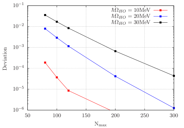
Figure 5: The convergence of $\delta_{D1}^{(0)}$ for $\mu^{2}$H as a function of $N_{\max}$ at different oscillator frequencies. The deviation is the fractional difference from the best estimate as in Eq. (3degmabbhbtdfdjdkeoewfdfefffsgs). Calculations are performed with the nuclear force from [55].

3.3 The effective interaction hyperspherical harmonic method ($A=3,4$)

To calculate the nuclear polarizability contribution to the spectrum of muonic atoms for nuclei with mass number $A=3,4$ we have used the EIHH method. The latter is a solver of the Schrödinger equation that expands the nuclear wave function on HH basis functions and utilizes an “effective interaction” to accelerate convergence. In the following subsections we first present the hyperspherical coordinates and hyperspherical harmonics, then outline the method of effective interaction. Full details of the method can be found in Refs. [49, 50].

3.3.1 Hyperspherical coordinates and hyperspherical harmonics

To separate the internal motion from the center of mass motion, the $A$-particle hyperspherical coordinates are defined by transformation of the relative Jacobi coordinates $\bm{\eta}_{1},\bm{\eta}_{2},\ldots\bm{\eta}_{A-1}$. In analogy with the spherical coordinates $(r,\hat{\Omega}_{2}=\hat{\bm{r}})$ in the two-body case, the $(3A-3)$ hyperspherical coordinates for $A$-particles are composed of one hyperradius,

$$\rho=\sqrt{\bm{\eta}_{1}^{2}+\bm{\eta}_{2}^{2}+\ldots+\bm{\eta}_{A-1}^{2}}\;,$$ (3degmabbhbtdfdjdkeoewfdfefffsgt)

and $(3A-4)$ hyperangular coordinates. Of the latter, $(2A-2)$ angular coordinates can be chosen to retain the Jacobi vector angles $\hat{\bm{\eta}}_{1},\hat{\bm{\eta}}_{2},\ldots\hat{\bm{\eta}}_{A-1}$. The remaining $(A-2)$ hyperangles are obtained by relating the norms of the Jacobi vector to $\rho$. For example, in the four-particle system we have three Jacobi vectors and two such hyperangles $\alpha_{1},\alpha_{2}$, defined through the relations

$$\eta_{1} =\rho\sin\alpha_{1}\,,$$ (3degmabbhbtdfdjdkeoewfdfefffsgu)

$$\eta_{2} =\rho\cos\alpha_{1}\sin\alpha_{2}\,,$$ (3degmabbhbtdfdjdkeoewfdfefffsgv)

$$\eta_{3} =\rho\cos\alpha_{1}\cos\alpha_{2}\,.$$ (3degmabbhbtdfdjdkeoewfdfefffsgw)

In short, the hyperspherical coordinates include one hyperradius $\rho$ and $(3A-4)$ hyperangles, which we collectively denote by $\hat{\Omega}_{A}$. Written in hyperspherical coordinates, any function of the Jacobi coordinates $f(\bm{\eta}_{1},\bm{\eta}_{2},...\bm{\eta}_{A-1})$ becomes $f(\rho,\hat{\Omega}_{A})$.

In analogy to the 3-dimensional case, the kinetic energy operator written in these coordinates is separated into a hyperradial part $\Delta_{\rho}$ and a hyper-centrifugal barrier $\hat{\bf K}_{A}^{2}/\rho^{2}$. Here, $\hat{\bf K}_{A}^{2}$ is the hyperangular momentum operator and depends on all the hyperangles. Accordingly, the internal Hamiltonian for an $A$-particle system reads ,

$$H_{\rm nucl}^{[A]}=-\frac{1}{2m}\Delta_{\rho}+\frac{1}{2m}\frac{\hat{\bf K}_{A}^{2}}{\rho^{2}}+V^{[A]}(\rho,\hat{\Omega}_{A})\,,$$ (3degmabbhbtdfdjdkeoewfdfefffsgx)

where $m$ is the mass of a single nucleon.

The hyperspherical harmonics $\cal Y_{[\it K]}$ are eigenfunctions of $\hat{\bf K}^{2}_{A}$ with eigenvalues $K(K+3A-5)$. They constitute a complete basis where one can expand the $A$-particle wave function. For the hyperradial part we use an expansion into Laguerre polynomials $L^{\alpha}_{n}(\rho)$ so that one has

$$\Psi(\rho,\hat{\Omega}_{A})=\sum_{n[K]}C_{n[K]}L^{\alpha}_{n}(\rho){\cal Y}_{[K]}(\hat{\Omega}_{A})\,.$$ (3degmabbhbtdfdjdkeoewfdfefffsgy)

Of course the nuclear wave function must be complemented by the spin-isospin parts. The whole function must be antisymmetric. This is a non-trivial task, that, however, has been solved in Refs. [56, 57].

3.3.2 The HH effective interaction

To accelerate the convergence of the HH expansion we substitute the bare nucleon-nucleon interaction with an effective interaction [58, 49, 50, 59]. To derive the effective interaction, the Hilbert space of the $A$-body Hamiltonian $H^{[A]}_{\rm nucl}=H^{[A]}_{0}+V^{[A]}$ is divided into a model space and a residual space, defined by the eigenprojectors $P$ and $Q$ of $H_{0}^{[A]}$,

$$[H_{0}^{[A]},P]=[H_{0}^{[A]},Q]=0\,;\,\,\,\,QH^{[A]}_{0}P=PH^{[A]}_{0}Q=0\,;\,\,\,\,P+Q=1\,.$$ (3degmabbhbtdfdjdkeoewfdfefffsgz)

The Hamiltonian $H^{[A]}_{\rm nucl}$ is then replaced by the effective model space Hamiltonian

$$H^{[A]{\rm eff}}=PH_{0}^{[A]}P+PV^{[A]{\rm eff}}P\;$$ (3degmabbhbtdfdjdkeoewfdfefffsha)

that by construction has the same energy levels as the low-lying spectrum of $H^{[A]}_{\rm nucl}$. In general, the effective interaction defined this way is an $A$-body interaction. Its construction is as difficult as finding the full-space solutions. Therefore, one has to approximate $V^{[A]{\rm eff}}$. However, one must build the approximate effective potential in such a way that it coincides with the bare one for $P\longrightarrow 1$, so that increasing the model space leads to a convergence of the eigenenergies and other observables to the true values. The EIHH method was developed along these lines.

In the EIHH approach we treat $\rho$ as parameter, and identify $H_{0}^{[A]}$ with the hyperspherical kinetic energy operator $\hat{\bf K}_{A}^{2}/\rho^{2}$. Therefore, the model space $P$ is spanned by all the $A$-body HH with $K\leq K_{\rm max}$. In order to construct the effective interaction we truncated it at the two body level, which we can easily solve, and calculate the two-body effective interaction $V^{[2]{\rm eff}}$ via the Lee-Suzuki similarity transformation method [60, 61]. The total effective interaction is then approximated as $V^{[A]{\rm eff}}\approx\sum_{i<j}^{A}V^{[2]{\rm eff}}_{ij}$. It should be noted that $V^{[A]{\rm eff}}$ is tailored for the HH model space and is constrained to coincide with the bare interaction in the limit $P\longrightarrow 1$.

For $A=3,4$ we have repeated the calculation with increasing values of $K_{\max}$ until satisfactory convergence was achieved. However, for these systems the number of HH basis states grows rather fast with $K_{\max}$ and therefore calculations were limited to values of $K_{\max}$ up to about 20. Nevertheless, even for a hard core nucleon-nucleon potential such as the Argonne $v_{18}$ (AV18) [55] we achieve a sub percent accuracy in $\delta_{\rm TPE}$. To demonstrate this point, the convergence of $\delta_{D1}^{(0)}$ in $\mu^{4}{\rm He}^{+}$ is presented in Fig. 6. Similarly to Fig. 5, we plot the deviation (3degmabbhbtdfdjdkeoewfdfefffsgs) as a function of $K_{\max}$. Comparing this figure with Fig. 5 the different convergence patterns are evident. Due to the effective interaction we first get a rapid convergence to $1\%$ level. Then the results start to oscillate around the asymptotic value and we see a much slower rate of convergence. The small decrease seen for the $K_{\max}=20$ point might be just coincidental.

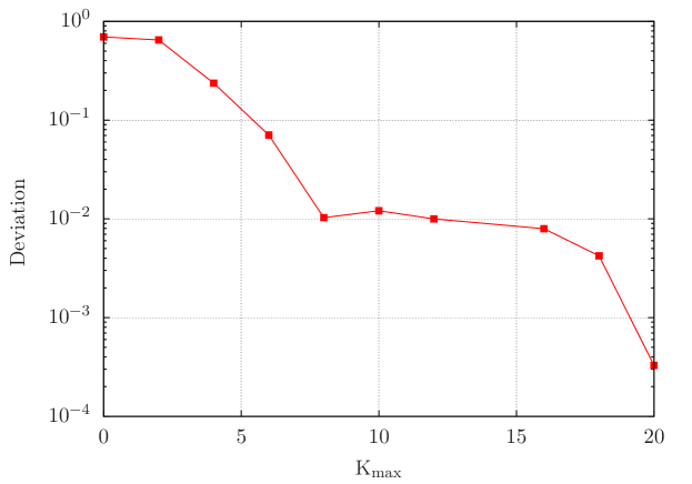
Figure 6: The convergence of $\delta_{D1}^{(0)}$ for $\mu^{4}{\rm He}^{+}$ as a function of $K_{\max}$. The deviation is the fractional difference from the best estimate, Eq. (3degmabbhbtdfdjdkeoewfdfefffsgs). Calculations are performed with the nuclear force from [55, 62].

4 Uncertainty estimation

The experimental precision in muonic atom Lamb shift measurements has achieved such a high level that, currently, the accuracy of the extracted nuclear charge radii is limited by the much larger uncertainties in the theoretical nuclear-structure corrections coming from the two-photon exchange process. For example, in $\mu^{3}{\rm He}^{+}$ theoretical uncertainties in $\delta_{\rm TPE}$ are five times larger than the experimental uncertainty, see Table 1. Because it is the limiting factor in the analysis of the Lamb shift experiments, it is of paramount importance to quantify the uncertainties in these theoretical calculations. To this end we trace and estimate all possible sources of uncertainty in the presented ab initio calculations. We regard each of the uncertainty sources as an independent variable and present its estimated standard deviation $\sigma$. Our total uncertainty estimate is computed as $\sigma_{\rm total}=\sqrt{\sigma_{1}^{2}+\sigma_{2}^{2}+\ldots\sigma_{n}^{2}}$ where $\sigma_{i}$ is the standard deviation of the $i\rm{th}$ uncertainty source. Below we list all considered error sources and explain their estimation method. Note that this is a global list of uncertainty sources, and each term does not necessarily apply to both $\delta^{A/N}_{\rm Zem}$ and $\delta^{A/N}_{\rm pol}$. The overall uncertainty in $\delta_{\rm TPE}$ is estimated by quadrature sum of the uncertainties in $\delta^{A}_{\rm TPE}$ and $\delta^{N}_{\rm TPE}$. Detailed results of uncertainty evaluation in each muonic atom will be given in Sections 5.5 and 5.6.

Numerical accuracy

To estimate the numerical accuracy, calculations are repeated for increasing model spaces until satisfactory convergence is reached. For the HO expansion ($A=2$), the model space is controlled by the parameter $N_{\rm max}$. For the EIHH method ($A=3,4$) the model space size is controlled by the maximal hyperangular momentum $K_{\rm max}$, as the hyperradial expansion converges rapidly. Accordingly, the numerical uncertainty is taken to be the difference between our best value and results obtained with lower $N_{\rm max}$ or $K_{\rm max}$ values.

For $A=3$, calculations with the $\chi$EFT nuclear potentials demonstrated slower convergence than for $A=4$. Therefore, in this case additional calculations were performed with the bare interaction, i.e., without applying the effective interaction mechanism described in Section 3.3.2. These calculations are variational and can be readily extrapolated. The final results are weighted averages of the effective interaction and bare results, with their respective uncertainty estimates.

Nuclear model

The nuclear potentials, which are derived from a phenomenological or effective rather than fundamental theory, introduce another source of uncertainty into the evaluation of the nuclear-structure corrections. A simple way to assess this uncertainty is to repeat the calculations with different potential models and compare the results. Following this strategy, for $A=3,4$ we employ in the nuclear Hamiltonian either one of the following state-of-the-art potentials: (i) the phenomenological AV18/UIX two-nucleon [55] plus three-nucleon [62] force; and (ii) a chiral effective field theory $\chi$EFT potential with two-nucleon [63] plus three-nucleon [64] force. Using the difference between these two calculations $\Delta$ to evaluate the nuclear-model uncertainty we interpret the value $\pm\Delta/\sqrt{2}$ as one standard deviation $1\sigma$.

For $A=2$, in Refs. [41, 31] we have performed a more comprehensive study of the nuclear theory uncertainties exploiting the power of the $\chi$EFT formulation. We have studied two sources of error: (1) the systematic uncertainty due to the freedom in the specific choice of the functional form of the potential [41], and (2) the statistical uncertainty due to the scatter in the nuclear input data used to fit nuclear forces [31]. $\chi$EFT, and effective field theories in general, furnish a systematic order-by-order description of low-energy processes. As such it can be utilized to estimate the systematic uncertainty of $\delta_{\rm TPE}$ by truncating at different chiral orders. At any given order, the $\chi$EFT low energy constants (LECs) are fitted to reproduce the appropriate nuclear data. Computational tools recently developed by Ekström et al. [65] allow an efficient study relating the scatter in the nuclear data to variations of the LECs. Analyzing these two effects, it was found that the variation of the LECs has negligible contribution to $\delta_{\rm TPE}$. The rigorously estimated systematic uncertainty in $\mu^{2}{\rm H}$ was found to be about 50$\%$ larger than what we have estimated in our simple approach comparing the AV18 potential and a $\chi$EFT interaction. This finding can hardly be extrapolated to $A=3$ and $4$, since due to the presence of three-nucleon forces in these nuclei, nuclear-model uncertainties are larger, as we shall see later.

Isospin symmetry breaking

Isospin symmetry is a useful concept in nuclear physics, however it is an approximate rather than an exact symmetry. In our calculations we have assumed that the total isospin $T$ is a conserved quantity and that all nucleons have equal mass, taking the average between proton and neutron masses. Ergo, isospin symmetry breaking (ISB) is another source of uncertainty in our calculations. In the $A=3$ nuclei, for example, most of the ISB effects can be accounted for by allowing the nuclear ground-state wave functions to include both total isospin channels $T=1/2,\;T=3/2$, and similarly for the intermediate states spanning the discretized continuum. This, however, increases the number of basis states in each calculation and the associated computational cost rises rapidly with $K_{\rm max}$. It was therefore carried out selectively only to estimate the uncertainty associated with performing isospin conserving calculations.

Nucleon-size corrections

As we explained in detail, finite nucleon-size effects are included in our calculations by expanding the neutron and proton form factors up to first order in $q^{2}$. Additional corrections are expected only for the Zemach and correlation terms that sum to $\delta^{(1)}_{\rm NR}$. The Zemach moment is roughly proportional to $r_{\rm nucl}^{3}\approx(r_{A}^{2}+\tilde{r}_{N}^{2})^{3/2}$, where $r_{A}$ denotes the point-proton radius and $\tilde{r}_{N}=(r_{p}^{2}+r_{n}^{2}N/Z)^{1/2}$. One can expand $r_{\rm nucl}^{3}$ in powers of $\tilde{r}_{N}/r_{A}$,

$$r_{\rm nucl}^{3}=r_{A}^{3}\left(1+\frac{3\tilde{r}_{N}^{2}}{2r^{2}_{A}}+\frac{3\tilde{r}_{N}^{4}}{8r_{A}^{4}}+\cdots\right),$$ (3degmabbhbtdfdjdkeoewfdfefffshb)

where the sub-sub-leading term is smaller than the leading one by a factor ${3\tilde{r}_{N}^{4}}/{8r_{A}^{4}}$, and is smaller than the subleading one by ${\tilde{r}_{N}^{2}}/{4r_{A}^{2}}$. To roughly estimate the higher-order nucleon-size correction to $\delta^{A}_{\rm Zem}$, we assign the error by

$$\sigma_{\rm NS}[\delta^{A}_{\rm Zem}]\approx{\rm max}\left(\frac{3\tilde{r}_{N}^{4}}{8r_{A}^{4}}|\delta^{(0)}_{Z3}|,\frac{\tilde{r}_{N}^{2}}{4r_{A}^{2}}|\delta^{(1)}_{Z1}|\right)~{}.$$ (3degmabbhbtdfdjdkeoewfdfefffshc)

Similarly, the nucleon-size uncertainty in $\delta^{A}_{\rm TPE}$ is estimated by replacing $\delta^{(1)}_{Z3}$ and $\delta^{(1)}_{Z1}$ in Eq. (3degmabbhbtdfdjdkeoewfdfefffshc) with $\delta^{(1)}_{R3}$ and $\delta^{(1)}_{R1}$ (or $\delta^{(1)}_{Z3}+\delta^{(1)}_{R3}$ and $\delta^{(1)}_{Z1}+\delta^{(1)}_{R1}$ for the case of $\delta^{A}_{\rm pol}$).

Relativistic corrections

As explained in Section 2.4, electric longitudinal and transverse relativistic corrections were included only for the leading non-relativistic term (keeping only the electric dipole contribution). Their sum turned out to be few percent of the non-relativistic value. We therefore estimate the uncertainty, due to the missing relativistic corrections to the higher-order contributions $\delta_{\rm NR}^{(2)}$ of the $\eta$-expansion, by assuming that they are of the same relative size with the ratio $|\delta^{(0)}_{L}+\delta^{(0)}_{T}|/|\delta^{(0)}_{D1}|$.

Coulomb corrections

Similarly to the relativistic corrections mentioned above, also the effect of Coulomb distortions was calculated only for the leading dipole term ($\delta^{(0)}_{C}$ is the Coulomb correction to $\delta^{(0)}_{D1}$ only). Also here, following Ref. [39], we estimate the uncertainty, due to missing Coulomb corrections to the higher-order contributions $\delta_{\rm NR}^{(2)}$, by assuming a similar relative size according to the ratio $|\delta^{(0)}_{C}/\delta^{(0)}_{D1}|$.

$\eta$ expansion

In Section 2.2 we have argued that the dimensionless parameter $\eta$ in the operator expansion is of order $\sqrt{m_{r}/m_{p}}$. We calculate terms up to second order in this expansion, i.e., the $(0)$, $(1)$ and $(2)$ contributions defined in Eqs. (3degmabar). This uncertainty, due to the omitted third-order corrections $(3)$ in the $\eta$-expansion, is roughly estimated based on the ratios between the calculated $(0)$, $(1)$ and $(2)$ contributions in each muonic atom. We are presently working on improving this uncertainty using other strategies, which give more rigorous estimates of the third-order corrections in the $\eta$-expansion. This will be relevant in particular for the $A=3$ systems, where this uncertainty is larger.

The $\bm{Z\alpha}$ expansion

Except for the logarithmically enhanced Coulomb distortion contribution, we include all terms of order $(Z\alpha)^{5}$ in our calculations of $\delta^{A}_{\rm pol}$. Since $Z\alpha$ is small for light muonic systems, the missing contribution from all the higher-order terms can be approximated by the next order in the series, $(Z\alpha)^{6}$, i.e., a correction to $\delta^{A}_{\rm pol}$ with a relative size that equals to $Z\alpha$, where $Z\alpha\simeq 0.7\%$ for $Z=1$, and $Z\alpha\simeq 1.5\%$ for $Z=2$.

Many-body currents

In chiral EFT, as the nuclear Hamiltonian admits an expansion in many-body operators, so do the electromagnetic operators. In our calculation we include only one-body operators for the electromagnetic charge and current operators, a procedure known as the impulse approximation. The effect of further corrections, i.e., two- and three-body currents, are expected to be very small and thus are neglected here. The reason is that the major contribution to $\delta^{A}_{\rm TPE}$ is due to Coulomb interactions between the muon and the nucleus. The latter depend mainly on the nuclear charge density operator. Many-body corrections to this operator appear in 4th order in the chiral expansion, and as such are expected to have a negligible effect on $\delta^{A}_{\rm TPE}$.

The magnetic dipole term $\delta^{(0)}_{M}$ comes from the current density operator instead, but it is very small. Nevertheless, we do include it and provide an update of its value for $A=2,3$ and new values for $A=4$ in this review. The correction to the magnetic-dipole one-body impulse approximation operator appears at 2nd order in the chiral expansion and enhance the strength of $\delta^{(0)}_{M}$ by about 10% for $A=2$, see, e.g., [66]. As we carried out our calculations of $\delta^{(0)}_{M}$ in the impulse approximation for all light muonic atoms, an uncertainty of 10$\%$ is assigned to $\delta^{(0)}_{M}$, which is negligible with respect to other uncertainty sources.

Hadronic corrections

For completeness we include in this presentation also the hadronic, i.e., neutron and proton TPE contributions to the muonic Lamb shift. As we did not carry these calculations ourselves, we adopt the uncertainties assigned in the respective references, scaled with the number of nucleons and the normalization constant $\phi^{2}(0)$.

5 Results

In this Section we will present an overview of results for light muonic systems, from muonic deuterium atoms to muonic helium ions. While we will primarily focus on our own contributions, we make an effort to put them in the context of other approaches. Apart from the very early and simplified studies performed in the 60’s [67], we will quote and compare both past and modern results from other groups and review them in the light of the new pressing quests raised after the emergence of the proton-radius puzzle. In these comparisons, special emphasis will be devoted to discussing uncertainties. For clarity, when quoting uncertainty values in percentage we will always specify whether we mean a $1\sigma$ or a $2\sigma$ error.

5.1 $\mu^{2}{\rm H}$

In muonic deuterium, the muon orbits the simplest possible compound nucleus, namely the deuteron, a hydrogen isotope made by a bound state of a proton and a neutron. Being a very simple nucleus, it has been studied extensively in the literature. The first theoretical studies of polarizability corrections for electronic/muonic deuterium using potential models date back to the 90’s. At that time, the experimental interest was directed towards understanding the isotope shift between ordinary hydrogen and deuterium atoms, where polarizability effects are small but not negligible. Their inclusion was in fact motivated by the striding progress of laser spectroscopy. Pachucki et al. [68] first used a square-well potential to approximate the nuclear force and shortly after, Lu and Rosenfelder [69] analyzed both electronic and muonic deuterium using simple separable nucleon-nucleon potentials that were lacking the one-pion exchange. The first to analyze the nuclear physics uncertainty on electronic and muonic deuterium were Leidemann and Rosenfelder [70]. They related $\delta_{\rm TPE}$ to the electromagnetic longitudinal and transverse response functions, following Rosenfelder’s original derivation [38], and implemented a variety of realistic nucleon-nucleon forces, at that time considered state-of-the-art. While they did not include Coulomb distortions and other terms, such as the intrinsic proton polarizability term, they observed that the uncertainty related to the nuclear force should be small and estimated it to be below 2$\%$.

Table 2: Comparison of nuclear polarizability contributions (in meV) for muonic deuterium taken from Refs. [36, 41, 39, 28]. For the first three columns, numbers are obtained with the AV18 potential. Refs.[36, 39] do not explicitly quote $\delta^{A}_{\rm Zem}$, but employ the cancellation of the corresponding elastic and inelastic terms in $\delta^{A}_{\rm TPE}$. For the purpose of this comparison, we show here the results on $\delta_{M}^{(0)}$ with the originally used truncated weight function ${\mathcal{F}}_{M}\approx\pi{\sqrt{2\omega/m_{r}}}$ and not the expression of Eq. (3degmabbhbtdfdjdkeoeu).

	Pachucki [36]	Hernandez et al. [41]	Pachucki and Wienczek [39]	Friar [28]
	(2011)	(2014)	(2015)	(2013)
$\delta^{(0)}_{D1}$	-1.910	-1.907	-1.910	-1.925
$\delta^{(0)}_{L}$	0.035	0.029	0.026	0.037
$\delta^{(0)}_{T}$	$-$	-0.012	$-$	$-$
$\delta_{HO}$	$-$	$-$	-0.004	$-$
$\delta^{(0)}_{C}$	0.261	0.262	0.261	$-$
$\delta^{(0)}_{M}$	0.016	0.008	0.008	0.011
$\delta^{(1)}_{Z3}$	$-$	0.357	$-$	$-$
$\delta^{(2)}_{R2}$	0.045	0.042	0.042	0.042
$\delta^{(2)}_{Q}$	0.066	0.061	0.061	0.061
$\delta^{(2)}_{D1D3}$	-0.151	-0.139	-0.139	-0.137
$\delta^{(1)}_{Z1}$	$-$	0.064	$-$	$-$
$\delta^{(1)}_{np}$	$-$	0.017	0.018	0.023
$\delta^{(2)}_{NS}$	$-$	-0.020	-0.020	-0.021
$\delta^{A}_{\rm pol}$	$-$	-1.240	$-$	$-$
$\delta^{A}_{\rm Zem}$	$-$	-0.421	$-$	$-$
$\delta^{A}_{\rm TPE}$	-1.638	-1.661	-1.657	-1.909

After the discovery of the proton radius puzzle in 2010 [1] and given that the CREMA collaboration planned to investigate other light muonic atoms, the subject gained a renewed interest. In 2011 Pachucki [36] published a thorough calculation of nuclear-structure corrections in muonic deuterium, which included relativistic corrections and Coulomb corrections. He used the modern realistic AV18 nucleon-nucleon potential in his calculations. In 2013 Friar [28] derived finite nucleon size corrections and analyzed muonic deuterium in zero-range theory, which allows for an analytical solution. With the correct asymptotic form of the $s$-wave deuteron wave function reproduced, this calculation is similar to pion-less effective field theory at next-to-leading order, whose nuclear-physics uncertainty is expected to be $1\sim 2\%$ based on a power counting analysis.

In 2014 [41] we presented our calculation of nuclear-structure corrections using modern nucleon-nucleon potentials derived from $\chi$EFT and pointed out that the effective field theory framework allows for a systematic analysis of uncertainties related to the non-perturbative nature of nuclear forces, which we estimated to be $0.6\%$. We also performed calculations with the AV18 potential and compared to Pachucki. After mutual verifications, the results agreed very nicely, as we show in Table 2. There, we provide a comparison of all the terms of Refs. [36, 41, 39, 28], where we neglect the single nucleon polarizability contribution. Despite the additional higher order terms included by Pachucki and Wienczek [39] (term denoted with $\delta_{HO}$) and the slight difference in the relativistic terms $\delta^{(0)}_{L}$ and $\delta^{(0)}_{T}$, the final calculations of $\delta^{A}_{\rm TPE}$ from Ref. [41] and [39], where there is almost a term-by-term correspondence, agree at the level of 0.25%. This is very reassuring since the derivation of the formulas and the numerical implementation were done by two independent groups .

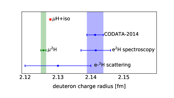
Figure 7: Deuteron radius puzzle: Recent determination of the deuteron charge radius from $\mu^{2}{\rm H}$ [22] in comparison to the CODATA evaluation of 2014 [5] and measurements from ordinary deuterium spectroscopy [71]. Also shown are the results obtained from electron scattering [72] and the value obtained combining isotope shift [73] with muonic hydrogen [1] data, denoted with “$\mu{\rm H}$+iso”. Figure adapted from Ref. [22].

In 2016, the CREMA collaboration released the muonic deuterium Lamb shift data [22]. In analogy to the proton case, the charge radius $r_{d}=2.12562(78)$ fm extracted from muonic deuterium revealed to be smaller, with a $6.0\sigma$ (or $7.5\sigma$) deviation from the world averaged CODATA 2014 [5] (or CODATA 2010 [2]) value. It also deviates by $3.5\sigma$ with respect to spectroscopic extractions from ordinary $e^{2}{\rm H}$ alone [71]. Different from the proton case, in the so-called “deuteron-radius puzzle” electron scattering data [72] are not precise enough to discriminate among muonic and electronic deuterium spectroscopy. By combining the radius squared difference $r_{d}^{2}-r_{p}^{2}$ measured from isotope shift experiments [73] with the absolute determinations of the proton radius from muonic hydrogen [1, 4], a value $r_{d}=2.12771(22)$ fm is obtained. This is denoted with “$\mu{\rm H}+$iso” in Fig. 7, where it is shown together with the other determinations. The “$\mu{\rm H}+$iso” result is very close to the absolute determination of muonic deuterium, but still differs from it by $2.6\sigma$. Such difference can be directly related to the $\delta_{\rm TPE}$ value used in the extraction of $r_{d}$ from muonic deuterium. In fact, from Eq. (1), one can see that by measuring $\delta_{\rm LS}$ and knowing $\delta_{\rm QED}$, it is possible to extract $\delta_{\rm TPE}$ from an experimentally determined radius. Using the $r_{d}$ from “$\mu{\rm H}+$iso” shown in Fig. 7 leads to an experimental value $\delta_{\rm TPE}=-1.7638(68)$ meV [22], which differs from the theoretical summary value of Krauth et al. [29] by $2.6\sigma$. In Ref. [22] it was argued that this might be due to missing contributions or underestimated uncertainties in the theoretical derivation of $\delta_{\rm TPE}$. It is to note that the theoretical summary value of Ref. [29] does not include only results from ab initio calculations, but also results from dispersion relation analyses [74], which despite suffering from a $35\%$ uncertainty, are compatible with the results obtained from ab initio calculations.

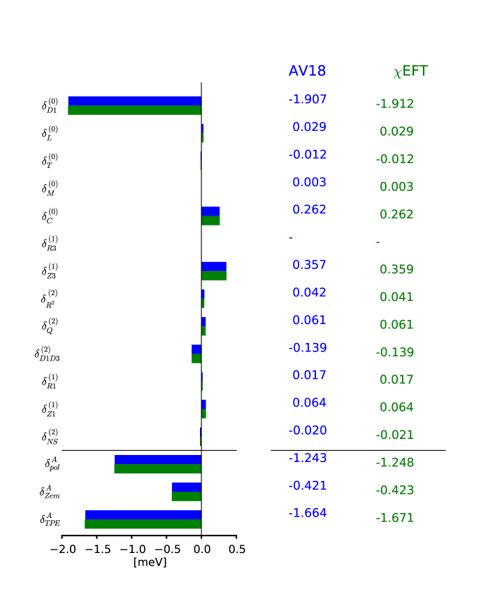
Figure 8: Graphic representation of the various contributions to $\delta^{A}_{\rm TPE}$ in the Lamb shift of $\mu^{2}{\rm H}$ calculated with the AV18 [55] and a $\chi$EFT potential [63]. Numerical values in meV are listed on the right.

Very recently, motivated by the above mentioned $2.6\sigma$ disagreement, we have analyzed statistical and systematic uncertainties in $\chi$EFT [31] and obtained a result consistent with our previous one, thus still differing from the experimental determination of $\delta_{\rm TPE}$. From an analysis of the various sources of uncertainties, we learned that statistical uncertainties from propagated LECs are small and that systematic uncertainties in nuclear potentials are well under control. Thus, we deduce that these deuteron discrepancies are unlikely to be explained by underestimated uncertainties in $\delta_{\rm TPE}$, at least at $(Z\alpha)^{5}$ presently considered. Recent work by Hill and Paz [12] pointed out that single nucleon contributions might have a larger error bar than previously estimated, thus affecting the deuteron radius puzzle. The actual size of single-nucleon uncertainties still remains debated [75, 76]. In order to further understand the origin of this difference, from the theoretical point of view it might be interesting to investigate higher order terms in the $Z\alpha$ expansion, which require to go beyond second order perturbation theory. Pachucki et al. [77] recently looked into three-photon exchange effects in muonic deuterium and found that their size is small and cannot explain the $2.6\sigma$ discrepancy.

In Figure 8, we show a graphic representation and the numerical results of various terms composing $\delta_{\rm TPE}$. Presented are values obtained with the AV18 potential and with the chiral nucleon-nucleon force at next-to-next-to-next-to leading order by Entem and Machleidt [63] denoted by $\chi$EFT. It is evident that the $\delta^{(0)}_{D1}$ term dominates and $\delta^{(1)}_{Z3}$ is the second important correction, about a factor of 5 smaller. With respect to $\delta^{A}_{\rm pol}$, the elastic Zemach term $\delta^{A}_{\rm Zem}$ is three times smaller.

To evaluate the total nuclear-model uncertainty (amounting to 0.6% as mentioned before) we did not just take the difference between the AV18 and one $\chi$EFT potential, but rather accounted for the dependence on various cutoffs of the chiral potentials and also estimated the uncertainty related to the chiral order truncation [31]. Including all the other sources of uncertainty, namely atomic physics, single nucleon contributions etc., as discussed in Section 4, the overall uncertainty of our muonic deuterium calculation amounts to 1.3$\%(1\sigma)$ on the full $\delta_{\rm TPE}$ [31]. Details on the separate single nucleon contributions will be shown later, in the summary of Tables 7 and 8, where we will compare muonic deuterium to other muonic systems analyzed in this review.

Finally, it is to note that in the various calculations of Refs. [36, 41, 39, 31], an operator expansion was used as described in Section 2.2. Such expansion is truncated at the second order, leading to the $(0)$, $(1)$ and the $(2)$ contributions. Going to third order in this expansion is very complicated and impractical. Thus, in a recent study, we performed a different expansion, very similar to the approach adopted by Leidemann and Rosenfelder [70], which is more reliable and allows to estimate the effects of third order corrections in the $\eta$-expansion. The latter are found to be $0.3\%$ of $\delta^{A}_{\rm TPE}$ for $\mu^{2}{\rm H}$ in the point-nucleon limit [78], see also Section 5.6.

5.2 $\mu^{3}{\rm H}$

In $\mu^{3}{\rm H}$ the muon orbits the triton nucleus, an hydrogen isotope made by a bound state of one proton and two neutrons. Triton is a radioactive isotope of hydrogen and as such muonic tritium has not yet been studied in the laboratory. While its radioactivity would not compromise safety when used in very small quantities for spectroscopic experiments, its low-energy $\beta$-decay emissions would produce a large background in the region where X-rays are measured in muonic atom experiments.

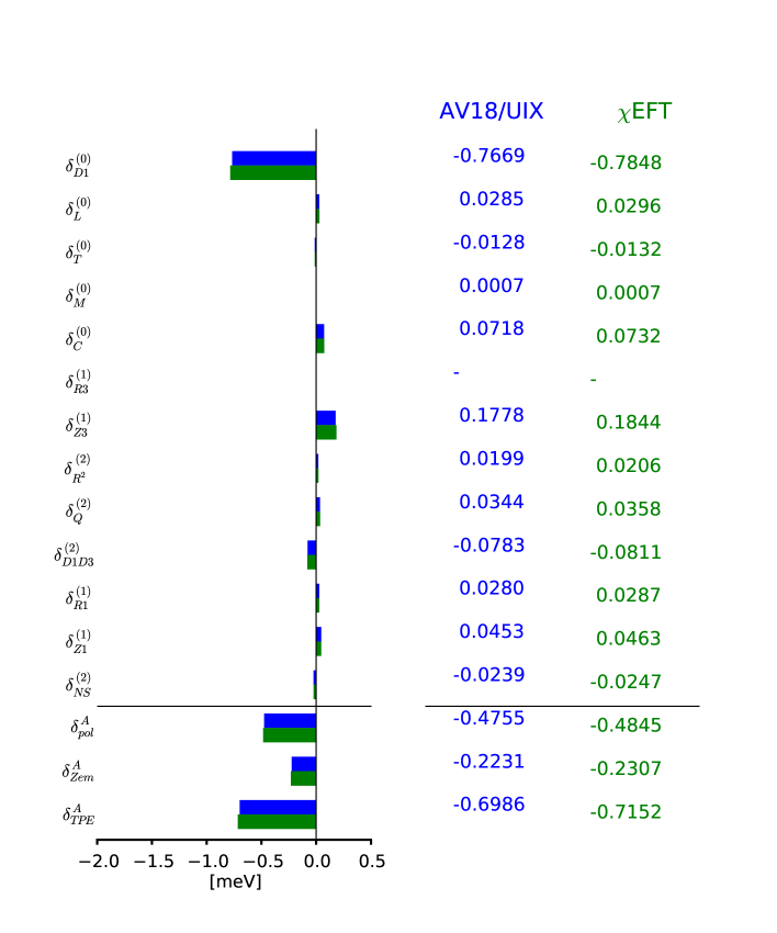
Figure 9: Graphic representation of the various contributions to $\delta^{A}_{\rm TPE}$ in the Lamb shift of $\mu^{3}{\rm H}$, calculated with the AV18+UIX [55, 62] and a $\chi$EFT nuclear Hamiltonian [63, 64]. Numerical values in meV are listed on the right.

From the theoretical point of view, solving a three-nucleon problem is more involved than solving the deuteron. The main difference is that one has to supplement the nuclear Hamiltonian with three-nucleon forces, which are less constrained with respect to the two-nucleon forces. Thus, one expects nuclear physics uncertainties to be larger than in muonic deuterium.

In 2016 we performed the first ab initio calculation of $\delta_{\rm TPE}$ for $\mu^{3}$H, mostly to investigate structure differences with respect to the muonic deuterium and its nuclear mirror system, namely muonic ³He⁺, which is discussed in the next subsection. As in the case of $\mu^{2}{\rm H}$, also for $\mu^{3}{\rm H}$ there is only one proton, thus all corrections are expected to be of the same order of magnitude due to their $Z\alpha$ dependence. However, the break-up threshold energies are different, with the triton’s being 6.28 MeV with respect to the deuteron’s 2.2 MeV. Since $\delta_{\rm TPE}$ is dominated by the dipole electric transitions and $\delta^{(0)}_{D1}$ has an inverse energy weight, one expects the polarizability effects to be smaller in muonic tritium than in muonic deuterium. Indeed, this is what we find.

In Fig. 9, we show our results for all the terms composing $\delta^{A}_{\rm TPE}$ calculated using two potential sets: the phenomenological AV18+UIX [55, 62] and one parameterization of the $\chi$EFT Hamiltonian[63, 64], both of which consist of two- and three-nucleon potentials. Similarly to what observed in $\mu^{2}{\rm H}$, $\delta^{(0)}_{D1}$ dominates also in $\mu^{3}{\rm H}$, with $\delta^{(1)}_{Z3}$ being the next important correction. With respect to $\delta^{A}_{\rm pol}$ the elastic Zemach term $\delta^{A}_{\rm Zem}$ in $\mu^{3}{\rm H}$ is only about a factor of two smaller, and not a factor of three as in $\mu^{2}{\rm H}$. This is mostly due to the smaller polarizability arising from the larger binding energy of ³H. Finally, the potential model dependence in nuclear-structure corrections to $\mu^{3}$H is of the order of 3$\%$ ($1\sigma$). The latter is enhanced with respect to $\mu^{2}{\rm H}$, due to the addition of the less constrained three-nucleon forces.

5.3 $\mu^{3}{\rm He}^{+}$

³He is an isotope of helium with two protons and one neutron. In muonic ³He⁺ a single muon orbits this nucleus, forming a positively charged ion. ³He is the mirror nuclear system with respect to ³H, where protons and neutrons are exchanged. It has a very similar break-up threshold energy, the only difference being the Coulomb interaction between the two protons. Even though the large $\delta^{(0)}_{D1}$ term has an inverse energy weight, the about 1 MeV difference in threshold energy will not lead to significant difference in nuclear-structure corrections to $\mu^{3}{\rm He}^{+}$ versus $\mu^{3}$H. On the contrary, what will make its TPE larger than in $\mu^{3}{\rm H}$ and $\mu^{2}{\rm H}$, is the $Z\alpha$ factor, with $Z$ being 2 for ³He, as opposed to 1 in ³H and ²H.

In recent times, the interest in nuclear-structure corrections to muonic ³He⁺ has been raised by the activities of the CREMA collaboration. Motivated by the above mentioned proton- and deuteron-radius puzzles, the collaboration has recently measured transitions in the $\mu^{3}{\rm He}^{+}$ [21], which are presently being analyzed. The charge radius of ³He can be extracted from Lamb shift measurements, provided that their nuclear polarizability is known with sufficient accuracy.

The prospects of obtaining an accurate charge radius for ³He is deemed even more interesting given that it will shed light on yet another radius puzzle pertaining to the isotope shift in ordinary helium atoms. Indeed, various $2S$–$2P$ atomic transitions in ordinary ³He and ⁴He have been measured by different groups. Via a combination of spectroscopic isotope shift data and accurate QED calculations, the difference in squared radii with respect to a reference nucleus, namely $\delta{r^{2}}=r^{2}_{{}^{3}{\rm He}}-r^{2}_{{}^{4}{\rm He}}$ in this case, can be extracted. The latest results on this matter were reported by Zheng et al. [79] and the present situation is displayed in Fig. 10. There, one can appreciate the discrepancy among the various measurements amounting, for example, to $4\sigma$ between the data from Cancio Pastor et al. [80] and Rooij et al. [81].

Figure 10: Isotope shift radius puzzle in ³He. Figure adapted from Ref. [79]. Experimental data are from Zheng et al. [79], Cancio Pastor et al [80], van Rooij et al. [81], and Shiner et al. [82].

The atomic physics community is very much looking forward to absolute radii determinations from muonic atoms, since such new data will have the potential to shed light on this isotope shift puzzle. To exclude either of the determinations presented in Fig. 10 by three respective standard deviations via Lamb shifts measurements, the latter should be determined with an accuracy of 1.5 meV [83]. Since in $\mu^{3}{\rm He}^{+}$ QED contributions are known with an uncertainty of only 0.04 meV and the experimental uncertainty is expected to be of 0.08 meV, the above requirement translates into a direct constraint on the $\delta_{\rm TPE}$, which should be known with an uncertainty of 1.5 meV or better. Given that the size of the total $\delta_{\rm TPE}$ is of about 15 meV, as we shall see below and in our Summary 5.6, this corresponds to a 10$\%$ accuracy.

Historically, the early computation by Rinker in 1976 [84], giving a total polarizability of $-4.9$ meV with a roughly estimated uncertainty of $20\%~{}(1\sigma)$, remained the last word on nuclear-structure corrections on $\mu^{3}{\rm He}^{+}$ for about 40 years. Of course, that large of an uncertainty would not allow to shed light on today’s isotope shift puzzle. In 2016, we calculated the full $\delta_{\rm TPE}$ in $\mu^{3}{\rm H}^{+}$ for the first time [32], providing a thorough estimate of the related uncertainties amounting to 2.5% ($1\sigma$). This was a dramatic reduction with respect to the previous estimate and is well below the requested 10% uncertainty to shed light on the isotope shift puzzle. Subsequently, Carlson et al. [83] applied their dispersion relation method to $\mu^{3}{\rm He}^{+}$. Thanks to the fact that good experimental data exist for the electromagnetic excitation of ³He, the uncertainties in $\delta_{\rm TPE}$ were quite reduced with respect to the deuteron case. While, a comparison of separate contributions may be less accurate due to the fact that ab initio and dispersion relation methods are very different, the total $\delta_{\rm TPE}$ are in nice agreement with each other, with $-15.46(39)$ meV from Ref. [32, 85] and -15.14(49) meV from Ref. [83]. In the summary [30] prepared in anticipation of the future analysis of $\mu^{3}{\rm He}^{+}$, the average value of the previous two has been chosen.

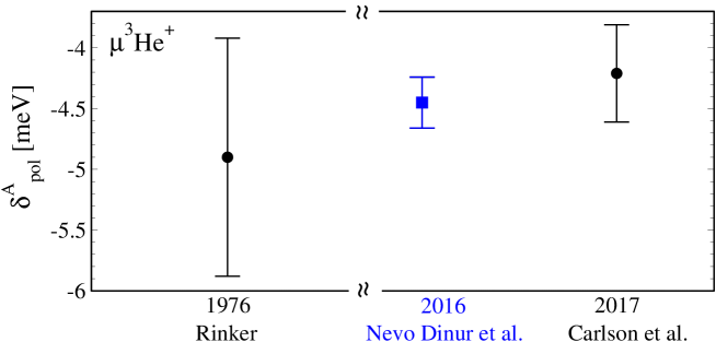
Figure 11: Time evolution of $\delta^{A}_{\rm pol}$ estimates for $\mu^{3}{\rm He}^{+}$ with corresponding $\pm 1\sigma$ uncertainties. The ab initio computation is denoted by the square. See text for details.

In Fig. 11, we present a historical overview of the calculations of $\delta^{A}_{\rm pol}$ in muonic ³He⁺. It is evident that ab initio computations provided so far the most precise determination. They are consistent with dispersion relation results which have only a slightly larger uncertainty. The precision by which we know $\delta_{\rm TPE}$ today will allow the CREMA collaboration to obtain a competitive measurement of the helium radii and discern among isotopic shifts data, which would not have been possible with the $20\%$ uncertainties of the older TPE calculation.

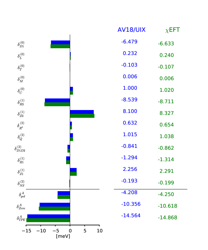
Figure 12: Same as Fig. 9 but for $\mu^{3}{\rm He}^{+}$.

In Fig. 12 we finally show our results for all the terms composing $\delta^{A}_{\rm TPE}$ using two potential sets: the phenomenological AV18+UIX [55, 62] and one parameterization of $\chi$EFT [63, 64]. As previously anticipated, nuclear-structure corrections are larger in $\mu^{3}{\rm He}^{+}$ than in $\mu^{3}$H due to the $Z$ dependence. Also in the $\mu^{3}{\rm He}^{+}$ case, $\delta^{(0)}_{D1}$ is the most important correction to $\delta_{\rm pol}^{A}$, since the two large terms appearing in $\delta^{(1)}_{\rm NR}$, namely $\delta^{(1)}_{R3}$ and $\delta^{(1)}_{Z3}$ are opposite in sign and mostly cancel out. As already mentioned in Section 2.2, $\delta^{(1)}_{R3}$ is different from zero only for $Z\neq 1$ nuclei, where more than one proton exists. The hierarchy in the various terms of the $\eta$-expansion is also preserved. For $\mu^{3}{\rm He}^{+}$, we note that $\delta^{A}_{\rm Zem}$ is larger than that of $\mu^{3}$H, mainly due to the $(Z\alpha)^{5}$ scaling and it is even larger than $\delta^{A}_{\rm pol}$.

5.4 $\mu^{4}{\rm He}^{+}$

In muonic ⁴He⁺, a single muon orbits a nucleus of ⁴He, also called alpha-particle, which is a bound state of two protons and two neutrons. Being a $Z=2$ nucleus, muonic ⁴He⁺ is a positively charged ion. Moreover since the nuclear spin is zero, the structure of its atomic spectrum is simplified, in that there is no hyperfine splitting. The QED theory of the Lamb shift and of the fine structure of muonic atoms with spinless nuclei, including $\mu^{4}{\rm He}^{+}$, was recently revisited in Ref. [86], to which we refer the interested reader.

The first studies of nuclear-structure corrections in $\mu^{4}{\rm He}^{+}$ date back to the 70’s, when the precision of contemporary experiments on muonic atoms performed at CERN [87] reached a level where it became necessary to take into account the effects of the internal excitation of the nucleus.

Various theorists tackled this issue, at first aiming to estimate these effects and only later at understanding the associated uncertainties. Bernabeau and Karlskog [88] used dispersion relations to connect the polarizability to electron scattering data even before the CERN experiment was performed and obtained a value of $-3.1$ meV, with no uncertainty estimates. Later Henley, Kriejs and Wilets [89] used a harmonic oscillator model to microscopically describe polarizability effects and obtained a value three times larger, namely $-13.1~{}{\rm meV}\leq\delta^{A}_{\rm pol}\leq-12.2$ meV. In 1976 Rinker [84] related polarizability corrections in muonic atoms to various measured electromagnetic transitions and obtained a value of $-3.1$ meV, compatible with Bernabeau and Karlskog, indicating that the value from Ref. [89] was wrong. His very rough uncertainty estimate was of about 20$\%$ ($1\sigma$). Finally Friar settled the situation by confirming that a reasonable estimate of nuclear polarizability and its uncertainty should be $-3.1\pm 20\%$ [90]. It should be noted that the fact that three of the early calculations obtained a value of 3.1 meV is partially a coincidence, since for example two inaccurate treatments were made by Bernabeau and Karlskog which canceled out, as pointed out by Friar.

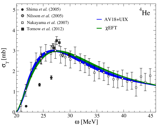
Figure 13: Photodisintegration cross section $\sigma_{\gamma}$ as a function of the energy transfer $\omega$: recent experimental data (dark circles from Ref. [91], light circles from Ref. [92], light squares from Refs. [93], and dark squares from Ref. [94, 95]) compared with theoretical calculations and corresponding uncertainty bands (dark band from Ref. [96] and light band from Ref. [97]). The relation of this cross section to the dipole response function is simply $\sigma_{\gamma}(\omega)=4\pi^{2}\alpha\omega S_{D1}(\omega)$. Figure adapted from Ref. [98].

In his work, Friar derived a connection between $\delta_{\rm TPE}$ to sum rules of the photoabsoprtion cross section $\sigma_{\gamma}$, which was known experimentally. He was the first to seriously discuss uncertainties, primarily related to the experimental data on photonuclear cross sections. Even today, if one tried to estimate nuclear-structure corrections from modern data on ⁴He, the situation would not be much different, as explained in Fig. 13. An up-to-date picture of recent experimental data is presented in comparison to theoretical calculations obtained with the Lorentz integral transform method using state-of-the-art realistic two- and three-nucleon potentials as input. One can readily see that experimental data differ from each other or suffer from large error bars. As a consequence the accuracy of the extracted $\delta_{\rm TPE}$, or better of the extracted dominant dipole contribution $\delta^{(0)}_{D1}$, would not be satisfactory. In Ref. [21], it was pointed out that in muonic helium, to determine the nuclear radii with a relative accuracy of $3\times 10^{-4}$, $\delta_{\rm TPE}$ needs to be known at the $\sim 5\%$ ($1\sigma$) level. It is evident from Fig. 13 that ab initio theory based on modern potentials has a real chance to provide us with the necessary accuracy.

In fact, in 2013 we provided the first ab initio computation of the full $\delta_{\rm TPE}$ [33] using the realistic nuclear Hamiltonian, AV18+UIX [55, 62] and one parameterization of $\chi$EFT [63, 64]. We have used the difference of the two potentials as a way to probe nuclear-model uncertainties, obtaining a 4$\%$ ($1\sigma$) effect. This indetermination comes mostly from what we call nuclear physics uncertainty and is very much connected to the fact that three-nucleon forces are less constrained than two-nucleon forces. The overall uncertainty budget, including atomic physics errors and other sources, is of $6\%$ ($1\sigma$).

In Fig. 14, the time evolution of $\delta^{A}_{\rm pol}$ estimates is shown, from the first calculations in the 70’ until now, leaving out the most likely wrong result of Ref. [89]. When the uncertainty was not estimated, it might be considerably large, and we indicate it by the dashed line. One can readily see that while the number has been coincidentally stable in the early calculations, our ab initio descriptions were the first to actually reduce the $1\sigma$ error bar from a $20\%$ to a $6\%$. This will allow for a sensible extraction of the charge radius from $\mu^{4}{\rm He}^{+}$ spectroscopic measurements by the CREMA collaboration.

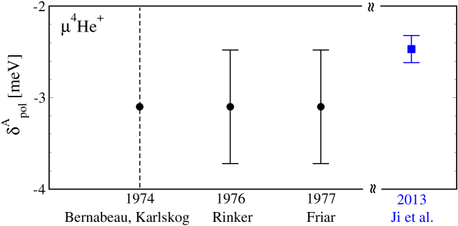
Figure 14: Time evolution of $\delta^{A}_{\rm pol}$ estimates for $\mu^{4}{\rm He}^{+}$ with corresponding $2\sigma$ uncertainties. In the earliest calculations uncertainties were not estimated and are potentially large as indicated by the dashed line. The ab initio result is indicated by the square symbol. See text for details.

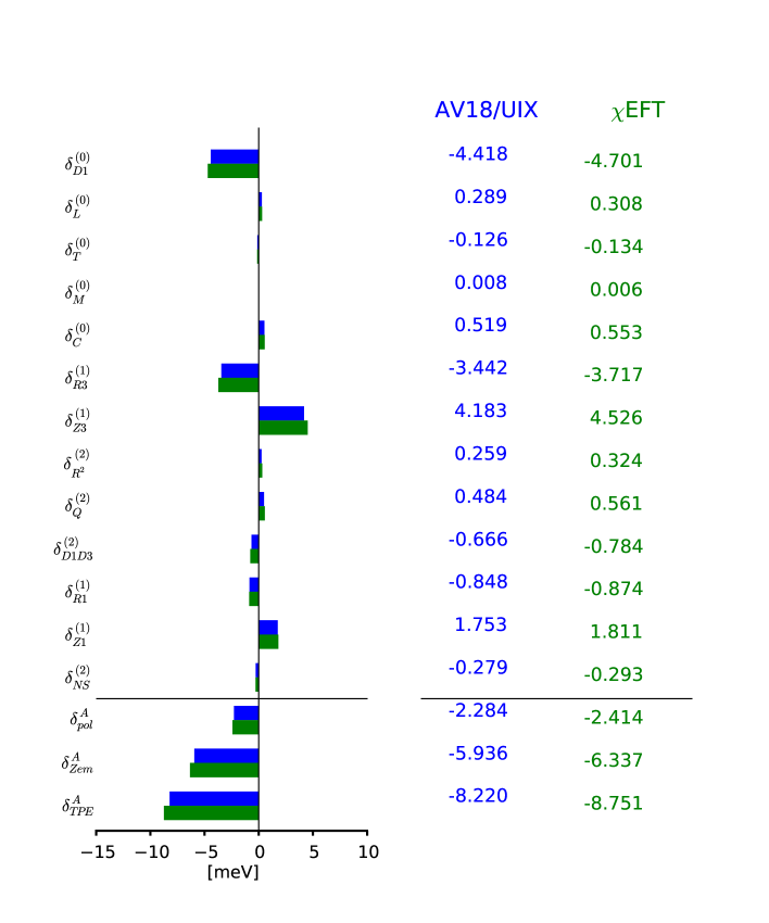
Figure 15: Same as Fig. 9 but for $\mu^{4}{\rm He}^{+}$.

Finally, our broken down $\delta^{A}_{\rm TPE}$ results with a few updates are shown in Fig. 15. We observe that $\delta^{(0)}_{D1}$ is again the dominant piece, with $\delta_{Z3}^{(1)}$ and $\delta^{(1)}_{R3}$ being opposite in sign and thus largely canceling out. The overall strengths of the various terms is very similar to the case of $\mu^{3}{\rm He}^{+}$.

We would like to emphasize that in this review we present the first results for the $\delta^{(0)}_{M}$ term in $\mu^{4}{\rm He}^{+}$, which were neglected in Ref. [33]. In this respect we provide here a more accurate calculations of the $\delta^{A}_{\rm TPE}$ and thus of the total $\delta_{\rm TPE}$.

5.5 Intrinsic nucleonic two-photon exchange

The evaluation of the hadronic part of the two-photon exchange contribution in muonic atoms is beyond the scope of nuclear ab initio calculations, in which the internal nucleonic degrees of freedom are not explicitly included.

Using dispersion relation analyses on electron-proton scattering data, $\delta_{\rm TPE}^{N}$ in $\mu{\rm H}$ is obtained as a combination of four components: elastic, non-pole Born, inelastic, and subtraction terms. For $\mu$H, Carlson and Vanderhaeghen obtained the elastic, non-pole Born, and inelastic terms to be respectively $-0.0295(13)$ meV, $0.0048$ meV, and $-0.0127(05)$ meV [99]. Using chiral perturbation theory, the subtraction term was calculated by Birse and McGovern to be $0.0042(10)$ meV [100]. The combination of elastic and non-pole Born contributions yields $\delta_{\rm Zem}^{N}$, and the sum of inelastic and subtraction terms gives $\delta_{\rm pol}^{N}$. The uncertainties are obtained in quadrature sum. Each contributions are shown in Table 3.

The dispersion relation was also applied to evaluate two-photon exchange effects in $\mu^{2}{\rm H}$ [74] and $\mu^{3}{\rm He}^{+}$ [83]. $\delta_{\rm TPE}$ in these muonic atoms are also separated into elastic, non-pole Born, inelastic, and subtraction terms under dispersion relation analysis. However, these contributions were given in Refs. [74, 83] with the nuclear and hadronic parts combined, with only a few exceptions. For comparison, we list in Table 3 only the explicit hadronic terms in $\mu^{2}{\rm H}$ and $\mu^{3}{\rm He}^{+}$ calculated by dispersion relation analyses.

Table 3: $\delta_{\rm TPE}^{N}$ (in meV) evaluated in dispersion relation analyses.

	$\mu{\rm H}$	$\mu^{2}{\rm H}$	$\mu^{3}{\rm He}^{+}$
$\delta^{N}_{\rm Zem}$	$-$0.0247(13)
$\delta^{N}_{\rm pol}$	$-$0.0085(11)		$-$0.10(4)
inelastic	$-$0.0127(05)	$-$0.028(2)	$-$0.31(2)
subtraction	0.0042(10)		0.21(3)
$\delta^{N}_{\rm TPE}$	$-$0.0332(17)

Using the scaling relations (3degmabbhbtdfdjdkeoewfdfefffsfz,3degmabbhbtdfdjdkeoewfdfefffsga), we can relate $\delta_{\rm Zem}^{N}$ and $\delta_{\rm pol}^{N}$ in $\mu{\rm H}$, evaluated in dispersion relation analyses, to the corresponding contributions in other light muonic atoms. The results are shown in Table 4. Regarding $\delta^{N}_{\rm Zem}$, the main difference across the various systems is given by the $Z^{4}$ scaling, slightly adjusted by an additional scaling from the muon reduced mass. The uncertainty of $\delta_{\rm Zem}^{N}$ is estimated based on that in $\mu{\rm H}$, multiplied with the scaling coefficient in Eq. (3degmabbhbtdfdjdkeoewfdfefffsfz).

Table 4: $\delta_{\rm TPE}^{N}$ contributions (in meV) to muonic atoms are calculated using scaling relation with $\delta_{\rm TPE}^{N}$ in $\mu{\rm H}$.

	$\mu^{2}{\rm H}$	$\mu^{3}{\rm H}$	$\mu^{3}{\rm He}^{+}$	$\mu^{4}{\rm He}^{+}$
$\delta^{N}_{\rm Zem}$	$-$0.030(02)	$-$0.033(02)	$-$0.52(03)	$-$0.54(03)
$\delta^{N}_{\rm pol}$	$-$0.020(10)	$-$0.031(17)	$-$0.25(13)	$-$0.34(20)
inelastic	$-$0.030(02)	$-$0.047(06)	$-$0.38(05)	$-$0.52(10)
subtraction	0.010(10)	0.016(16)	0.12(12)	0.17(17)
$\delta^{N}_{\rm TPE}$	$-$0.050(10)	$-$0.064(17)	$-$0.77(14)	$-$0.89(20)

To compare with the dispersion relation analyses, we separate $\delta^{N}_{\rm pol}$ into inelastic and subtraction terms, which are both obtained by the scaling relation in Eq. (3degmabbhbtdfdjdkeoewfdfefffsga). The inelastic part of $\delta^{N}_{\rm pol}$ in $\mu^{2}{\rm H}$ is $-0.030$ meV, compared to $-0.028$ meV from dispersion relation analyses. We consider this difference, $\sigma_{\rm med}^{N}(\mu^{2}{\rm H})\equiv 0.002$ meV, as a result of nuclear medium effects and nucleon-nucleon interferences, neglected in Eq. (3degmabbhbtdfdjdkeoewfdfefffsga). We assume the medium effect in another muonic atom/ion $\mu{\rm X}$ is amplified by a factor of $A(A-1)/2$, considering the number of nucleon-nucleon pairs inside nucleus $X$. Therefore, the uncertainty of the inelastic term is estimated by

$$\sigma^{N}_{\rm inel}(\mu{\rm X}) = \left\{\left[A\frac{\phi_{\mu{}{\rm X}}^{2}(0)}{\phi^{2}_{\mu{\rm H}}(0)}\sigma^{N}_{\rm inel}(\mu{\rm H})\right]^{2}+\left[\frac{A(A-1)}{2}\frac{\phi^{2}_{\mu{}{\rm X}}(0)}{\phi^{2}_{\mu^{2}{\rm H}}(0)}\sigma^{N}_{\rm med}(\mu^{2}{\rm H})\right]^{2}\right\}^{1/2}$$ (3degmabbhbtdfdjdkeoewfdfefffshd)

$$= AZ^{3}\left\{\frac{m_{r}^{6}(\mu{\rm X})}{m_{r}^{6}(\mu{\rm H})}\left[\sigma^{N}_{\rm inel}(\mu{\rm H})\right]^{2}+\frac{(A-1)^{2}m_{r}^{6}(\mu{\rm X})}{4\,m_{r}^{6}(\mu^{2}{\rm H})}\left[\sigma^{N}_{\rm med}(\mu^{2}{\rm H})\right]^{2}\right\}^{1/2}{.}$$ (3degmabbhbtdfdjdkeoewfdfefffshe)

The evaluation of the subtraction term is generally model dependent. Similar values of the subtraction term in $\mu{\rm H}$ were obtained in Refs. [99, 11, 12, 75, 76], only its uncertainty being disputed. We follow the strategy of Ref. [29] by assigning a $\pm 100\%$ error to the subtraction term in muonic atoms. The uncertainties in $\delta^{N}_{\rm pol}$ and $\delta^{N}_{\rm TPE}$ are then obtained by using relevant quadrature sums. Our results of hadronic terms in $\mu^{3}{\rm He}^{+}$ are consistent with those obtained in dispersion relation analysis [83].

5.6 Summary

In this summary we will compare all light muonic atoms discussed above against each other and include single nucleon contributions to provide values for the total $\delta_{\rm TPE}$.

Table 5: Nuclear-structure corrections to the Lamb shift (in meV), broken down into all terms composing $\delta^{A}_{\rm TPE}$. All light muonic atoms are computed here with AV18/UIX nuclear potential (in case of the deuteron only AV18).

	$\mu^{2}{\rm H}$	$\mu^{3}{\rm H}$	$\mu^{3}{\rm He}^{+}$	$\mu^{4}{\rm He}^{+}$
$\delta^{(0)}_{D1}$	$-$1.907	$-$0.7669	$-$6.479	$-$4.418
$\delta^{(0)}_{L}$	0.029	0.0285	0.232	0.289
$\delta^{(0)}_{T}$	$-$0.012	$-$0.0128	$-$0.103	$-$0.126
$\delta^{(0)}_{M}$	0.003	0.0007	0.006	0.008
$\delta^{(0)}_{C}$	0.262	0.0718	1.000	0.519
$\delta^{(1)}_{R3}$	0	0	$-$8.539	$-$3.442
$\delta^{(1)}_{Z3}$	0.357	0.1778	8.100	4.183
$\delta^{(2)}_{R^{2}}$	0.042	0.0199	0.632	0.259
$\delta^{(2)}_{Q}$	0.061	0.0344	1.015	0.484
$\delta^{(2)}_{D1D3}$	$-$0.139	$-$0.0783	$-$0.841	$-$0.666
$\delta^{(1)}_{R1}$	0.017	0.0280	$-$1.294	$-$0.848
$\delta^{(1)}_{Z1}$	0.064	0.0453	2.256	1.753
$\delta^{(2)}_{NS}$	$-$0.020	$-$0.0239	$-$0.193	$-$0.279
$\delta^{A}_{\rm pol}$	$-$1.243	$-$0.4755	$-$4.208	$-$2.284
$\delta_{\rm Zem}^{A}$	$-$0.421	$-$0.2231	$-$10.356	$-$5.936
$\delta^{A}_{\rm TPE}$	$-$1.664	$-$0.6986	$-$14.564	$-$8.220

Table 6: Same as in Table 5, but for one parameterization of the $\chi$EFT nuclear potential (in case of the deuteron only nucleon-nucleon interaction). Numbers are given in meV.

	$\mu^{2}{\rm H}$	$\mu^{3}{\rm H}$	$\mu^{3}{\rm He}^{+}$	$\mu^{4}{\rm He}^{+}$
$\delta^{(0)}_{D1}$	$-$1.912	$-$0.7848	$-$6.633	$-$4.701
$\delta^{(0)}_{L}$	0.029	0.0296	0.240	0.308
$\delta^{(0)}_{T}$	$-$0.012	$-$0.0132	$-$0.107	$-$0.134
$\delta^{(0)}_{M}$	0.003	0.0007	0.006	0.006
$\delta^{(0)}_{C}$	0.262	0.0732	1.020	0.553
$\delta^{(1)}_{R3}$	0	0	$-$8.711	$-$3.717
$\delta^{(1)}_{Z3}$	0.359	0.1844	8.327	4.526
$\delta^{(2)}_{R^{2}}$	0.041	0.0206	0.654	0.324
$\delta^{(2)}_{Q}$	0.061	0.0358	1.038	0.561
$\delta^{(2)}_{D1D3}$	$-$0.139	$-$0.0811	$-$0.862	$-$0.784
$\delta^{(1)}_{R1}$	0.017	0.0287	$-$1.314	$-$0.874
$\delta^{(1)}_{Z1}$	0.064	0.0463	2.291	1.811
$\delta^{(2)}_{NS}$	$-$0.021	$-$0.0247	$-$0.199	$-$0.293
$\delta^{A}_{\rm pol}$	$-$1.248	$-$0.4845	$-$4.250	$-$2.414
$\delta_{\rm Zem}^{A}$	$-$0.423	$-$0.2307	$-$10.618	$-$6.337
$\delta^{A}_{\rm TPE}$	$-$1.671	$-$0.7152	$-$14.868	$-$8.751

First, in Tables 5 and 6 we detail all the terms composing $\delta^{A}_{\rm TPE}$ computed with the AV18/UIX and $\chi$EFT potentials, respectively. While these numerical values have already been shown in Figs. 8, 9, 12 and 15, these new tables allow for a comparison of the different light muonic systems. Indeed, one primarily appreciates the $Z$ dependence, which is making each term of $\mu^{3}{\rm He}^{+}$ and $\mu^{4}{\rm He}^{+}$ larger than the corresponding one in $\mu^{2}{\rm H}$ and $\mu^{3}{\rm H}$. Looking at $\delta_{\rm TPE}^{A}$, it is also interesting to note that overall nuclear-structure corrections due to the few-nucleon dynamics are the largest in $\mu^{3}{\rm He}^{+}$ and the smallest in $\mu^{3}{\rm H}$. This fact is simply explained by a combination of the $Z$ dependence and differences in nuclear threshold effects, as we have argued above.

Table 7: Contributions to $\delta_{\rm TPE}$ of the Lamb shift in light muonic atoms (in meV), with separated contributions from the few-nucleon dynamics and from the individual nucleons. The uncertainty associated with each value is given in brackets. Due to cancellation of the elastic and inelastic Zemach term, the uncertainty in $\delta_{\rm TPE}$ can differ from the quadrature sum of the corresponding terms in the table.

	$\delta^{A}_{\rm Zem}$	$\delta^{A}_{\rm pol}$	$\delta^{N}_{\rm Zem}$	$\delta^{N}_{\rm pol}$	$\delta_{\rm TPE}$
$\mu^{2}{\rm H}$	$-$0.423(04)	$-$1.245(13)	$-$0.030(02)	$-$0.020(10)	$-$1.718(17)
$\mu^{3}{\rm H}$	$-$0.227(06)	$-$0.480(11)	$-$0.033(02)	$-$0.031(17)	$-$0.771(22)
$\mu^{3}{\rm He}^{+}$	$-$10.49(23)	$-$4.23(18)	$-$0.52(03)	$-$0.25(13)	$-$15.49(33)
$\mu^{4}{\rm He}^{+}$	$-$6.14(31)	$-$2.35(13)	$-$0.54(03)	$-$0.34(20)	$-$9.37(44)

In Table 7 we include the intrinsic single nucleon contributions to each muonic system by adding $\delta^{N}_{\rm Zem}$ and $\delta^{N}_{\rm pol}$, so as to compose the total $\delta_{\rm TPE}$. Values and uncertainties of the single nucleon terms are given in subsection 5.5. They do not depend on the $A$-nucleon dynamics, nor on the potential. One can observe that generally single nucleon contributions to $\delta_{\rm TPE}$ are smaller than the parts determined by the few-nucleon dynamics, thus making it crucial to reliably determine the latter and the related uncertainties. As demonstrated above for each light muonic atom, ab initio computations of the few-nucleon dynamics have enabled to reach a precision level which was not available before. The uncertainty associated with each value of Table 7 for $\delta^{A}_{\rm pol},\delta^{A}_{\rm Zem}$ and $\delta^{A}_{\rm TPE}$ is given in the brackets and in Table  8 is broken down into all the uncertainties sources explained in Section 4. In particular, it is to note that while for $\mu^{2}{\rm H}$ the largest source of uncertainty comes from atomic physics, for $\mu^{4}{\rm He}^{+}$ it comes from nuclear modeling.

Table 8: Relative uncertainties (in $\%$) for $\delta^{A}_{\rm pol}$, $\delta^{A}_{\rm Zem}$, and $\delta^{A}_{\rm TPE}$. The estimation is based on sources of uncertainty listed in Section 4. The total uncertainties are obtained from a quadrature sum.

	$\mu^{2}{\rm H}$			$\mu^{3}{\rm H}$			$\mu^{3}{\rm He}^{+}$			$\mu^{4}{\rm He}^{+}$
	$\delta_{\rm pol}^{A}$	$\delta_{\rm Zem}^{A}$	$\delta_{\rm TPE}^{A}$	$\delta_{\rm pol}^{A}$	$\delta_{\rm Zem}^{A}$	$\delta_{\rm TPE}^{A}$	$\delta_{\rm pol}^{A}$	$\delta_{\rm Zem}^{A}$	$\delta_{\rm TPE}^{A}$	$\delta_{\rm pol}^{A}$	$\delta_{\rm Zem}^{A}$	$\delta_{\rm TPE}^{A}$
Numerical	0.0	0.0	0.0	0.1	0.0	0.1	0.4	0.1	0.1	0.4	0.3	0.4
Nuclear model	0.3	0.5	0.4	1.3	2.4	1.7	0.7	1.8	1.5	3.9	4.6	4.4
ISB	0.2	0.2	0.2	0.7	0.2	0.5	1.8	0.2	0.5	2.2	0.5	0.5
Nucleon size	0.3	0.8	0.0	0.6	0.9	0.2	1.2	1.3	0.9	2.7	2.0	1.2
Relativistic	0.0	-	0.0	0.1	-	0.1	0.4	-	0.1	0.1	-	0.0
Coulomb	0.4	-	0.3	0.5	-	0.3	3.0	-	0.9	0.4	-	0.1
$\eta$-expansion	0.4	-	0.3	1.3	-	0.9	1.1	-	0.3	0.8	-	0.2
Higher $Z\alpha$	0.7	-	0.5	0.7	-	0.5	1.5	-	0.4	1.5	-	0.4
Total	1.0	0.9	0.8	2.3	2.2	2.0	4.2	2.2	2.1	5.5	5.1	4.6

6 Conclusions

In this work we reviewed our recent activities devoted to the calculation of nuclear-structure corrections in light muonic atoms. This subject has gained a renewed interest following the emergence of the proton-radius puzzle and the subsequent experimental campaign of the CREMA collaboration directed towards Lamb shift measurements in light muonic systems, with the goal of extracting their nuclear charge radii and compare them to ordinary atom spectroscopy or electron scattering data.

While $\delta_{\rm TPE}$ is not a “traditional” observable for ab initio nuclear theory studies, we showed that, taking advantage of methodologies and few-body techniques developed for nuclear-structure physics, it could be computed with unprecedented precision. In particular, for the $\mu^{3}{\rm He}^{+}$ and $\mu^{4}{\rm He}^{+}$ we have reduced uncertainties by a factor of $5$, when compared to the previously available estimates of $\delta^{A}_{\rm pol}$. For $\mu^{2}{\rm H}$, instead, we have presented the most thorough estimates of the uncertainty related to the non-perturbative nature of nuclear forces. These achievements are crucial for the muonic atom measurements, where $\delta_{\rm TPE}$ is needed for the extraction of nuclear charge radii and is presently the bottle-neck to exploit the experimental precision.

State-of-the-art calculations of $\delta_{\rm{TPE}}$ presented in this work employ nuclear potentials derived either phenomenologically or from a low-energy expansion of quantum chromodynamics, namely $\chi$EFT. Effective field theories in general, unlike phenomenological models, furnish a systematic, i.e, order-by-order, description of low-energy processes at a chosen level of resolution. $\chi$EFT presently constitutes the modern paradigm of analyzing nuclear forces, which are built from a sum of pion-exchange contributions and nucleon contact terms, see, e.g., Refs. [101, 102]. Power counting enables to determine the importance of individual terms in the low-energy expansion and thereby also facilitates a meaningful truncation of higher-order diagrams that build the potential. Given the chiral expansion, contributions with a low power are more important than terms at higher powers. Starting from the leading order (LO), higher orders are denoted as next-to-leading order (NLO), next-to-next-to-leading (N²LO), etc. At each order of the chiral EFT potential, there is a finite set of parameters, the LECs, that determine the strength of various pion-nucleon and multi-nucleon operators. The LECs are not provided by the theory itself but can be obtained from fitting to selected experimental data, such as NN and $\pi$N scattering cross sections, and other few-body ground state observables, such as binding energies. Different fitting procedures exist, which in turn lead to different potentials. The optimal way to exploit such an approach is to explore an ensemble of parameterization of the potentials to probe both statistical and systematic uncertainties, order by order. We have performed such a study so far only for $\mu^{2}{\rm H}$ [31]. Remarkably, we find that statistical errors are small and that systematic errors are underestimated by maximally 50% when comparing only one choice of $\chi$EFT potential with a phenomenological interaction. This result cannot be easily extrapolated to the three and four-body systems. There, in fact three-body forces need to be included, which are much less constrained than the nucleon-nucleon force. Nevertheless, we expect that our calculations based on two substantially different interactions should capture the bulk of the uncertainty. A more thorough systematic and statistical analysis is useful and is presently called for.

It is to be noted that the nuclear theory community is at the moment devoting a fair amount of resources towards the development of nucleon-nucleon forces at N⁵LO and three-body forces at N⁴LO. In the future, these will potentially provide the possibility to reduce uncertainties in $\delta_{\rm TPE}$. A reduction of the uncertainties may be also obtained by fitting the LECs to radii extracted from muonic atoms with high precision. This strategy is presently under discussion.

One has to keep in mind that uncertainties on $\delta_{\rm TPE}$ are much larger than the experimental precision, as shown in Table 1 in the introduction to this review. As opposed to what is possible today for $\delta_{\rm QED}$, reducing nuclear-model uncertainties in $\delta_{\rm TPE}$ at the level of being able to match or even supersede the experimental precision is currently unrealistic and infeasible. The results presented in this review represent the state-of-the-art, some improvement might be achieved by exploring the pathways alluded to above, or by systematically adding the effect of meson exchange currents.

On the other hand, the CREMA collaboration aims at measuring the Lamb shift also in muonic lithium and beryllium ions. In preparation for that, the QED community has already started to calculate the corresponding QED corrections, see, e.g., [103]. The TPE contributions are presently based on rough estimates from the Rinker semi-empirical formula and/or from experimental data, as explained in Ref. [104]. They do not contain all the terms we derived in this review and are plagued by large uncertainties. For example, for $\mu^{6}{\rm Li}^{2+}$ the uncertainty is of 27% ($1\sigma$). Computing $\delta_{\rm TPE}$ in such systems with ab initio methods should be possible, and this would almost certainly lead to a reduction in the related uncertainty. Obviously, this does not come without challenges since ⁶Li has a pronounced ⁴He-²H cluster structure, so that very large model spaces are needed to capture these features when using basis function expansions. First steps towards developing the necessary machinery to achieve these computations are presently underway.

Another natural extension of this work is to explore nuclear-structure corrections to other transitions relevant in muonic atom spectroscopy, e.g., the hyperfine splitting. While $\mu{\rm H}$ is the first system that will be measured by several groups around the world (Switzerland, England and Japan), eventually also the hyperfine splitting in $\mu^{3}{\rm He}^{+}$ and $\mu^{2}{\rm H}$ will be investigated by the CREMA collaboration. We are presently in the process of deriving the necessary formalism to achieve this goal.

Finally, we would like to remark that in precision physics it is of paramount importance that different methods are employed to compute the $\delta_{\rm TPE}$ corrections and compared to the approach presented in this review. For example, the work based on dispersion relation is very relevant and, depending on the available experimental data, can reach comparable precision to the ab initio approach. Also, pion-less effective field theories may be applied to this problem, as well as other few-body methods that can deal with precise calculation of the response function.

Appendix A Wigner-Eckart Theorem

The reduced matrix element is defined by Wigner-Eckart Theorem [37] as

$$\langle N_{0}J_{0}M_{0}|T^{(k)}_{\nu}|NJM\rangle=(-1)^{k-J+J_{0}}\frac{\langle k\nu JM|J_{0}M_{0}\rangle}{\sqrt{2J_{0}+1}}\langle N_{0}J_{0}||T^{(k)}||NJ\rangle{,}$$ (3degmabbhbtdfdjdkeoewfdfefffshf)

$$\langle NJM|T^{(k)\dagger}_{\nu}|N_{0}J_{0}M_{0}\rangle=(-1)^{k}\frac{\langle k\nu JM|J_{0}M_{0}\rangle}{\sqrt{2J_{0}+1}}\langle NJ||T^{(k)}||N_{0}J_{0}\rangle{.}$$ (3degmabbhbtdfdjdkeoewfdfefffshg)

$$\langle NJ||T^{(k)}||N_{0}J_{0}\rangle=(-1)^{J-J_{0}}\langle N_{0}J_{0}||T^{(k)}||NJ\rangle^{*}{.}$$ (3degmabbhbtdfdjdkeoewfdfefffshh)

Using the relations in Eqs. (3degmabbhbtdfdjdkeoewfdfefffshf, 3degmabbhbtdfdjdkeoewfdfefffshg, 3degmabbhbtdfdjdkeoewfdfefffshh), we have

$$\sum\limits_{M}\langle N_{0}J_{0}M_{0}|A^{(k)}|NJM\rangle\cdot\langle NJM|B^{(k)}|N_{0}J_{0}M_{0}\rangle$$ (3degmabbhbtdfdjdkeoewfdfefffshi)

$$= \frac{(-1)^{J_{0}-J}}{2J_{0}+1}\langle N_{0}J_{0}||A^{(k)}||NJ\rangle\langle NJ||B^{(k)}||N_{0}J_{0}\rangle$$

$$= \frac{1}{2J_{0}+1}\langle N_{0}J_{0}||A^{(k)}||NJ\rangle\,\langle NJ||B^{(k)\dagger}||N_{0}J_{0}\rangle{,}$$

$$\langle N_{0}J_{0}|A^{(k)}|NJ\rangle\cdot\langle NJ|A^{(k)}|N_{0}J_{0}\rangle = \frac{1}{2J_{0}+1}|\langle N_{0}J_{0}||A^{(k)}||NJ\rangle|^{2}{.}$$ (3degmabbhbtdfdjdkeoewfdfefffshj)

The matrix element of the scalar product of two tensor operators obeys Eq. (7.1.6) in Ref. [37], which yields

$$\sum_{J^{\prime}M^{\prime}}|\langle j_{1}^{\prime}j_{2}^{\prime}J^{\prime}M^{\prime}|T^{(k)}\cdot U^{(k)}|j_{1}j_{2}JM\rangle|^{2}=\left\{\begin{array}[]{ccc}j_{1}^{\prime}&k&j_{1}\\ j_{2}&J&j_{2}^{\prime}\end{array}\right\}^{2}\,|\langle j_{1}^{\prime}||T^{(k)}||j_{1}\rangle|^{2}\,|\langle j_{2}^{\prime}||U^{(k)}||j_{2}\rangle|^{2}{.}$$ (3degmabbhbtdfdjdkeoewfdfefffshm)

A single operator in coupled scheme obeys Eq. (7.1.7) in Ref. [37], which leads to

$$|\langle j_{1}^{\prime}j_{2}J^{\prime}||T^{(k)}||j_{1}j_{2}J\rangle|^{2}=(2J+1)(2J^{\prime}+1)\left\{\begin{array}[]{ccc}j_{1}^{\prime}&J^{\prime}&j_{2}\\ J&j_{1}&k\end{array}\right\}^{2}|\langle j_{1}^{\prime}||T^{(k)}||j_{1}\rangle|^{2}{,}$$ (3degmabbhbtdfdjdkeoewfdfefffsho)

$$\langle\ell_{0}||Y_{k}||\ell\rangle=(-1)^{\ell_{0}}\sqrt{\frac{(2\ell_{0}+1)(2k+1)(2\ell+1)}{4\pi}}\left(\begin{array}[]{ccc}\ell_{0}&k&\ell\\ 0&0&0\end{array}\right){,}$$ (3degmabbhbtdfdjdkeoewfdfefffshp)

with $\left(:::\right)$ indicates the 3j-symbol. For $k=1$, we have

$$|\langle\ell_{0}||Y_{1}||\ell\rangle|^{2}=\frac{3}{4\pi}\left[(\ell_{0}+1)\delta_{\ell,\ell_{0}+1}+\ell_{0}\delta_{\ell,\ell_{0}-1}\right]{.}$$ (3degmabbhbtdfdjdkeoewfdfefffshq)

Appendix B Coulomb integrals

The radial Coulomb Green’s function $g_{\ell}$ can be expressed in the form of Whittaker functions [26] as

$$g_{\ell}(-\omega_{N};r,r^{\prime})=-2m_{r}\xi\frac{\Gamma(\ell+1-2\kappa)}{\Gamma(2\ell+2)}\,\mathcal{M}_{2\kappa,\ell+\frac{1}{2}}\left(\frac{r_{<}}{\xi}\right)\,\mathcal{W}_{2\kappa,\ell+\frac{1}{2}}\left(\frac{r_{>}}{\xi}\right){,}$$ (3degmabbhbtdfdjdkeoewfdfefffshr)

where $\kappa\equiv\frac{Z\alpha}{4}\sqrt{\frac{2m_{r}}{\omega_{N}}}$ and $\xi=1/\sqrt{8m_{r}\omega_{N}}$ are defined. The function $\mathcal{M}$ and $\mathcal{W}$ are two Whittaker functions, which are regular respectively at $r\rightarrow 0$ and $r\rightarrow\infty$. $g_{\ell}$ is therefore regular at both origin and infinity. The Whittaker functions satisfy the Wronskian relation that [26]

$$\mathcal{M}\frac{d\mathcal{W}}{dr}-\mathcal{W}\frac{d\mathcal{M}}{dr}=-\frac{\Gamma(2\ell+2)}{\xi\Gamma(\ell+1-2\kappa)}{.}$$ (3degmabbhbtdfdjdkeoewfdfefffshs)

In Section 2.3, we only need to evaluate the Coulomb integral $\mathcal{F}_{01}$, which can be analytically solved by using generating functions based on the double-Laplace transform of the Green’s function [105, 106]. This solution is related to the hypergeometric function ${}_{2}F_{1}$ by

$$\mathcal{F}_{01}(\omega_{N}) = \int_{0}^{\infty}dr\,\int_{0}^{\infty}dr^{\prime}R_{20}\left(\frac{m_{r}Z\alpha r}{2}\right)\;R_{20}\left(\frac{m_{r}Z\alpha r^{\prime}}{2}\right)\;\frac{g_{\ell}(-\omega_{N};r,r^{\prime})}{rr^{\prime}}$$ (3degmabbhbtdfdjdkeoewfdfefffsht)

$$= -\frac{1}{Z\alpha}\left[\frac{3}{4}-\frac{1}{4\kappa^{2}}+\frac{24\kappa(1-\kappa)}{(1+\kappa)^{6}}\,{}_{2}F_{1}\left(4,2-2\kappa,3-2\kappa,\frac{(1-\kappa)^{2}}{(1+\kappa)^{2}}\right)\right]{.}$$

Expanding $\mathcal{F}_{01}$ in powers of $\kappa$ yields,

$$\mathcal{F}_{01} = -\frac{1}{Z\alpha}\left[4\kappa+16\kappa^{2}\ln(4\kappa)+2\kappa^{2}+\mathcal{O}(\kappa^{3})\right]$$ (3degmabbhbtdfdjdkeoewfdfefffshu)

$$= -\sqrt{\frac{2m_{r}}{\omega_{N}}}-\frac{Z\alpha m_{r}}{\omega}\ln\frac{2(Z\alpha)^{2}m_{r}}{\omega}-\frac{Z\alpha m_{r}}{4\omega}+\cdots{.}$$

References

References

- [1] Pohl R et al. 2010 Nature 466 213–216 URL http://dx.doi.org/10.1038/nature09250
- [2] Mohr P J, Taylor B N and Newell D B 2012 Rev. Mod. Phys. 84(4) 1527–1605 URL http://link.aps.org/doi/10.1103/RevModPhys.84.1527
- [3] Lamb W E and Retherford R C 1947 Phys. Rev. 72(3) 241–243 URL http://link.aps.org/doi/10.1103/PhysRev.72.241
- [4] Antognini A et al. 2013 Science 339 417–420 URL http://www.sciencemag.org/content/339/6118/417.abstract
- [5] Mohr P J, Newell D B and Taylor B N 2016 Rev. Mod. Phys. 88(3) 035009 URL http://link.aps.org/doi/10.1103/RevModPhys.88.035009
- [6] Sick I 2003 Phys. Lett. B 576 62 – 67 URL http://www.sciencedirect.com/science/article/pii/S0370269303015387
- [7] Blunden P G and Sick I 2005 Phys. Rev. C 72(5) 057601 URL http://link.aps.org/doi/10.1103/PhysRevC.72.057601
- [8] Sick I 2018 Atoms 6 2 (Preprint 1801.01746)
- [9] Bernauer J C et al. 2010 Phys. Rev. Lett. 105(24) 242001 URL http://link.aps.org/doi/10.1103/PhysRevLett.105.242001
- [10] Zhan X et al. 2011 Phys. Lett. B 705 59 – 64 URL http://www.sciencedirect.com/science/article/pii/S0370269311012342
- [11] Miller G A 2013 Phys. Lett. B 718 1078 – 1082 URL http://www.sciencedirect.com/science/article/pii/S0370269312011677
- [12] Hill R J and Paz G 2017 Phys. Rev. D 95(9) 094017 URL https://link.aps.org/doi/10.1103/PhysRevD.95.094017
- [13] Pohl R, Gilman R, Miller G A and Pachucki K 2013 Annu. Rev. Nucl. Part. Sci. 63 175–204 URL http://dx.doi.org/10.1146/annurev-nucl-102212-170627
- [14] Beyer A et al. 2017 Science 358 79–85 URL http://science.sciencemag.org/content/358/6359/79
- [15] Fleurbaey H et al. 2018 Phys. Rev. Lett. 120(18) 183001 URL https://link.aps.org/doi/10.1103/PhysRevLett.120.183001
- [16] Gasparian A et al. 2012 Jefferson Lab Exp. E12–11–106 URL http://www.jlab.org/exp_prog/proposals/11/PR12-11-106.pdf
- [17] Meziane M (PRad Collaboration) 2013 AIP Conference Proceedings 1563 183–186 URL http://scitation.aip.org/content/aip/proceeding/aipcp/10.1063/1.4829405
- [18] Mihovilovič M and Merkel H (A1-Collaboration) 2013 AIP Conference Proceedings 1563 187–190 URL http://scitation.aip.org/content/aip/proceeding/aipcp/10.1063/1.4829406
- [19] Gilman R et al. (MUSE Collaboration) (Preprint 1303.2160)
- [20] Gilman R 2013 AIP Conference Proceedings 1563 167–170 URL http://scitation.aip.org/content/aip/proceeding/aipcp/10.1063/1.4829401
- [21] Antognini A et al. 2011 Can. J. of Phys. 89 47–57 URL http://dx.doi.org/10.1139/P10-113
- [22] Pohl R et al. 2016 Science 353 669–673 URL http://science.sciencemag.org/content/353/6300/669
- [23] Borie E and Rinker G A 1982 Rev. Mod. Phys. 54(1) 67–118 URL http://link.aps.org/doi/10.1103/RevModPhys.54.67
- [24] Borie E 2012 Annals of Physics 327 733 – 763 see arXiv:1103.1772v7 for an update, URL http://www.sciencedirect.com/science/article/pii/S0003491611001904
- [25] Eides M I, Grotch H and Shelyuto V A 2001 Physics Reports 342 63 – 261 URL http://www.sciencedirect.com/science/article/pii/S0370157300000776
- [26] Friar J 1979 Annals of Physics 122 151 – 196 URL http://www.sciencedirect.com/science/article/pii/0003491679903002
- [27] Zemach A C 1956 Phys. Rev. 104(6) 1771–1781 URL http://link.aps.org/doi/10.1103/PhysRev.104.1771
- [28] Friar J L 2013 Phys. Rev. C 88(3) 034003 URL http://link.aps.org/doi/10.1103/PhysRevC.88.034003
- [29] Krauth J J, Diepold M, Franke B, Antognini A, Kottmann F and Pohl R 2016 Annals of Physics 366 168–196 URL http://www.sciencedirect.com/science/article/pii/S0003491615004303
- [30] Franke B, Krauth J J, Antognini A, Diepold M, Kottmann F and Pohl R 2017 Eur. Phys. J. D 71 341 URL https://doi.org/10.1140/epjd/e2017-80296-1
- [31] Hernandez O, Ekström A, Dinur N N, Ji C, Bacca S and Barnea N 2018 Physics Letters B 778 377 – 383 URL https://www.sciencedirect.com/science/article/pii/S0370269318300510
- [32] Nevo Dinur N, Ji C, Bacca S and Barnea N 2016 Physics Letters B 755 380 – 386 URL http://www.sciencedirect.com/science/article/pii/S0370269316001192
- [33] Ji C, Nevo Dinur N, Bacca S and Barnea N 2013 Phys. Rev. Lett. 111(14) 143402 URL http://link.aps.org/doi/10.1103/PhysRevLett.111.143402
- [34] Diepold M, Krauth J J, Franke B, Antognini A, Kottmann F and Pohl R 2016 (Preprint 1606.05231)
- [35] Friar J L and Payne G L 1997 Phys. Rev. A 56(6) 5173–5175 URL http://link.aps.org/doi/10.1103/PhysRevA.56.5173
- [36] Pachucki K 2011 Phys. Rev. Lett. 106(19) 193007 URL http://link.aps.org/doi/10.1103/PhysRevLett.106.193007
- [37] Edmonds A 1996 Angular Momentum in Quantum Mechanics Investigations in physics (Princeton University Press) ISBN 9780691025896 URL http://books.google.ca/books?id=XzIlngEACAAJ
- [38] Rosenfelder R 1983 Nucl. Phys. A 393 301 – 313 URL http://www.sciencedirect.com/science/article/pii/0375947483901446
- [39] Pachucki K and Wienczek A 2015 Phys. Rev. A 91(4) 040503 URL https://link.aps.org/doi/10.1103/PhysRevA.91.040503
- [40] Walecka J 2004 Theoretical nuclear and subnuclear physics, second edition (Imperial college Press and World Scientific Pub.CompanyLimited) ISBN 9789812387950 URL http://books.google.ca/books?id=j1WUQgAACAAJ
- [41] Hernandez J O, Ji C, Bacca S, Nevo Dinur N and Barnea N 2014 Physics Letters B 736 344 – 349 URL http://www.sciencedirect.com/science/article/pii/S0370269314005413
- [42] Patrignani C et al. (Particle Data Group) 2016 Chinese Physics C 40 100001 URL http://stacks.iop.org/1674-1137/40/i=10/a=100001
- [43] Kamada H et al. 2001 Phys. Rev. C 64(4) 044001 URL https://link.aps.org/doi/10.1103/PhysRevC.64.044001
- [44] Leidemann W and Orlandini G 2013 Prog. Part. Nucl. Phys. 68 158–214 URL http://www.sciencedirect.com/science/article/pii/S014664101200110X
- [45] Efros V D, Leidemann W and Orlandini G 1994 Phys. Lett. B 338 130 – 133 URL http://www.sciencedirect.com/science/article/pii/0370269394913552
- [46] Efros V D, Leidemann W, Orlandini G and Barnea N 2007 Journal of Physics G: Nuclear and Particle Physics 34 R459 URL http://stacks.iop.org/0954-3899/34/i=12/a=R02
- [47] Nevo Dinur N, Barnea N, Ji C and Bacca S 2014 Phys. Rev. C 89(6) 064317 URL https://link.aps.org/doi/10.1103/PhysRevC.89.064317
- [48] Whitehead R, Watt A and Kelvin D 1980 Physics Letters B 89 313 – 315 URL http://www.sciencedirect.com/science/article/pii/0370269380901318
- [49] Barnea N, Leidemann W and Orlandini G 2000 Phys. Rev. C 61(5) 054001 URL http://link.aps.org/doi/10.1103/PhysRevC.61.054001
- [50] Barnea N, Leidemann W and Orlandini G 2001 Nucl. Phys. A 693 565 – 578 URL http://www.sciencedirect.com/science/article/pii/S0375947401007941
- [51] Lanczos C 1950 J. Res. Natl. Bur. Stand. B 45 255–282 URL https://doi.org/10.6028/jres.045.026
- [52] Haxton W C, Nollett K M and Zurek K M 2005 Phys. Rev. C 72(6) 065501 URL https://link.aps.org/doi/10.1103/PhysRevC.72.065501
- [53] Caurier E, Poves A and Zuker A P 1995 Phys. Rev. Lett. 74(9) 1517–1520 URL https://link.aps.org/doi/10.1103/PhysRevLett.74.1517
- [54] Messiah A 1965 Quantum Mechanics, Vol. 1 (North-Holland)
- [55] Wiringa R B, Stoks V G J and Schiavilla R 1995 Phys. Rev. C 51(1) 38–51 URL https://link.aps.org/doi/10.1103/PhysRevC.51.38
- [56] Barnea N and Novoselsky A 1997 Annals of Physics 256 192–225 URL http://www.sciencedirect.com/science/article/pii/S0003491697956736
- [57] Barnea N and Novoselsky A 1998 Phys. Rev. A 57(1) 48–58 URL https://link.aps.org/doi/10.1103/PhysRevA.57.48
- [58] Navrátil P and Barrett B R 1998 Phys. Rev. C 57(2) 562–568 URL https://link.aps.org/doi/10.1103/PhysRevC.57.562
- [59] Hjorth-Jensen M, Engeland T, Holt A and Osnes E 1994 Physics Reports 242 37–69 URL http://www.sciencedirect.com/science/article/pii/0370157394901406
- [60] Suzuki K and Lee S Y 1980 Progress of Theoretical Physics 64 2091–2106 URL http://dx.doi.org/10.1143/PTP.64.2091
- [61] Suzuki K and Okamoto R 1983 Progress of Theoretical Physics 70 439–451 URL http://dx.doi.org/10.1143/PTP.70.439
- [62] Pudliner B S, Pandharipande V R, Carlson J and Wiringa R B 1995 Phys. Rev. Lett. 74(22) 4396–4399 URL http://link.aps.org/doi/10.1103/PhysRevLett.74.4396
- [63] Entem D R and Machleidt R 2003 Phys. Rev. C 68(4) 041001 URL http://link.aps.org/doi/10.1103/PhysRevC.68.041001
- [64] Navrátil P 2007 Few-Body Systems 41 117–140 URL http://dx.doi.org/10.1007/s00601-007-0193-3
- [65] Carlsson B D, Ekström A, Forssén C, Strömberg D F, Jansen G R, Lilja O, Lindby M, Mattsson B A and Wendt K A 2016 Phys. Rev. X 6(1) 011019 URL https://link.aps.org/doi/10.1103/PhysRevX.6.011019
- [66] Hernandez O J, Bacca S and Wendt K A 2017 PoS BORMIO2017 041 URL https://doi.org/10.22323/1.302.0041
- [67] Joachain C 1961 Nuclear Physics 25 317 – 327 URL http://www.sciencedirect.com/science/article/pii/0029558261901626
- [68] Pachucki K, Leibfried D and Hänsch T W 1993 Phys. Rev. A 48(1) R1–R4 URL https://link.aps.org/doi/10.1103/PhysRevA.48.R1
- [69] Lu Y and Rosenfelder R 1993 Phys. Lett. B 319 7 – 12 erratum-ibid. B 333, 564 (1994) URL http://www.sciencedirect.com/science/article/pii/037026939390772A
- [70] Leidemann W and Rosenfelder R 1995 Phys. Rev. C 51(1) 427–430 URL http://link.aps.org/doi/10.1103/PhysRevC.51.427
- [71] Pohl R et al. 2017 Metrologia 54 L1 URL http://stacks.iop.org/0026-1394/54/i=2/a=L1
- [72] Sick I and Trautmann D 1998 Nucl. Phys. A 637 559–575 URL http://www.sciencedirect.com/science/article/pii/S0375947498003340
- [73] Parthey C G et al. 2010 Phys. Rev. Lett. 104(23) 233001 URL http://link.aps.org/doi/10.1103/PhysRevLett.104.233001
- [74] Carlson C E, Gorchtein M and Vanderhaeghen M 2014 Phys. Rev. A 89(2) 022504 URL http://link.aps.org/doi/10.1103/PhysRevA.89.022504
- [75] Birse M C and McGovern J A 2017 (Preprint 1708.09341)
- [76] Hill R J and Paz G 2017 (Preprint 1711.00893)
- [77] Pachucki K, Patkos V and Yerokhin V A 2018 (Preprint 1803.10313)
- [78] Hernandez O J et al. In preparation
- [79] Zheng X, Sun Y R, Chen J J, Jiang W, Pachucki K and Hu S M 2017 Phys. Rev. Lett. 119(26) 263002 URL https://link.aps.org/doi/10.1103/PhysRevLett.119.263002
- [80] Cancio Pastor P, Consolino L, Giusfredi G, De Natale P, Inguscio M, Yerokhin V A and Pachucki K 2012 Phys. Rev. Lett. 108(14) 143001 URL https://link.aps.org/doi/10.1103/PhysRevLett.108.143001
- [81] van Rooij R, Borbely J S, Simonet J, Hoogerland M D, Eikema K S E, Rozendaal R A and Vassen W 2011 Science 333 196–198 URL http://science.sciencemag.org/content/333/6039/196
- [82] Shiner D, Dixson R and Vedantham V 1995 Phys. Rev. Lett. 74(18) 3553–3556 URL https://link.aps.org/doi/10.1103/PhysRevLett.74.3553
- [83] Carlson C E, Gorchtein M and Vanderhaeghen M 2017 Phys. Rev. A 95(1) 012506 URL https://link.aps.org/doi/10.1103/PhysRevA.95.012506
- [84] Rinker G A 1976 Phys. Rev. A 14(1) 18–29 URL http://link.aps.org/doi/10.1103/PhysRevA.14.18
- [85] Hernandez J O, Nevo Dinur N, Ji C, Bacca S and Barnea N 2016 Hyper. Int. 237 158 URL https://doi.org/10.1007/s10751-016-1371-9
- [86] Korzinin E Y, Shelyuto V A, Ivanov V G and Karshenboim S G 2018 Phys. Rev. A 97(1) 012514 URL https://link.aps.org/doi/10.1103/PhysRevA.97.012514
- [87] Bertin A et al. 1975 Physics Letters B 55 411 – 414 URL http://www.sciencedirect.com/science/article/pii/037026937590372X
- [88] Bernabeu J and Jarlskog C 1974 Nucl. Phys. B 75 59 – 71 URL http://www.sciencedirect.com/science/article/pii/0550321374904647
- [89] Henley E, Krejs F and Wilets L 1976 Nuclear Physics A 256 349 – 361 URL http://www.sciencedirect.com/science/article/pii/0375947476903778
- [90] Friar J L 1977 Phys. Rev. C 16(4) 1540–1548 URL http://link.aps.org/doi/10.1103/PhysRevC.16.1540
- [91] Shima T et al. 2005 Phys. Rev. C 72(4) 044004 URL https://link.aps.org/doi/10.1103/PhysRevC.72.044004
- [92] Nilsson B et al. 2005 Physics Letters B 626 65–71 URL http://www.sciencedirect.com/science/article/pii/S0370269305012050
- [93] Nakayama S et al. 2007 Phys. Rev. C 76(2) 021305 URL https://link.aps.org/doi/10.1103/PhysRevC.76.021305
- [94] Tornow W et al. 2012 Phys. Rev. C 85(6) 061001 URL https://link.aps.org/doi/10.1103/PhysRevC.85.061001
- [95] Raut R et al. 2012 Phys. Rev. Lett. 108(4) 042502 URL https://link.aps.org/doi/10.1103/PhysRevLett.108.042502
- [96] Gazit D, Bacca S, Barnea N, Leidemann W and Orlandini G 2006 Phys. Rev. Lett. 96(11) 112301 URL http://link.aps.org/doi/10.1103/PhysRevLett.96.112301
- [97] Quaglioni S and Navrátil P 2007 Physics Letters B 652 370–375 URL http://www.sciencedirect.com/science/article/pii/S0370269307007642
- [98] Bacca S and Pastore S 2014 Journal of Physics G: Nuclear and Particle Physics 41 123002 URL http://stacks.iop.org/0954-3899/41/i=12/a=123002
- [99] Carlson C E and Vanderhaeghen M 2011 Phys. Rev. A 84(2) 020102 URL http://link.aps.org/doi/10.1103/PhysRevA.84.020102
- [100] Birse M and McGovern J 2012 Eur. Phys. J. A 48 120 URL http://dx.doi.org/10.1140/epja/i2012-12120-8
- [101] Epelbaum E, Glöckle W and Meißner U G 2005 Nucl. Phys. A 747 362–424 URL http://www.sciencedirect.com/science/article/pii/S0375947404010747
- [102] Machleidt R and Entem D 2011 Physics Reports 503 1 – 75 URL http://www.sciencedirect.com/science/article/pii/S0370157311000457
- [103] Krutov A A, Martynenko A P, Martynenko F A and Sukhorukova O S 2016 Phys. Rev. A 94(6) 062505 URL https://link.aps.org/doi/10.1103/PhysRevA.94.062505
- [104] Drake G W F and Byer L L 1985 Phys. Rev. A 32(2) 713–719 URL https://link.aps.org/doi/10.1103/PhysRevA.32.713
- [105] Bodine C and Gaskell R W 1982 Journal of Mathematical Physics 23 2217–2220 URL https://doi.org/10.1063/1.525310
- [106] Swainson R A and Drake G W F 1991 Journal of Physics A: Mathematical and General 24 95 URL http://stacks.iop.org/0305-4470/24/i=1/a=020