Variational inference for sparse network reconstruction from count data

Abstract

In multivariate statistics, the question of finding direct interactions can be formulated as a problem of network inference - or network reconstruction - for which the Gaussian graphical model (GGM) provides a canonical framework. Unfortunately, the Gaussian assumption does not apply to count data which are encountered in domains such as genomics, social sciences or ecology.

To circumvent this limitation, state-of-the-art approaches use two-step strategies that first transform counts to pseudo Gaussian observations and then apply a (partial) correlation-based approach from the abundant literature of GGM inference. We adopt a different stance by relying on a latent model where we directly model counts by means of Poisson distributions that are conditional to latent (hidden) Gaussian correlated variables. In this multivariate Poisson lognormal-model, the dependency structure is completely captured by the latent layer. This parametric model enables to account for the effects of covariates on the counts.

To perform network inference, we add a sparsity inducing constraint on the inverse covariance matrix of the latent Gaussian vector. Unlike the usual Gaussian setting, the penalized likelihood is generally not tractable, and we resort instead to a variational approach for approximate likelihood maximization. The corresponding optimization problem is solved by alternating a gradient ascent on the variational parameters and a graphical-Lasso step on the covariance matrix.

We show that our approach is highly competitive with the existing methods on simulation inspired from microbiological data. We then illustrate on three various data sets how accounting for sampling efforts via offsets and integrating external covariates (which is mostly never done in the existing literature) drastically changes the topology of the inferred network.

Keywords: multivariate count data $\cdot$ Poisson-lognormal distribution $\cdot$ Gaussian graphical models $\cdot$ variational inference $\cdot$ sparsity $\cdot$ graphical-Lasso

1 Introduction

Networks are the de facto mathematical object used to model and represent pairwise interactions between entities of interest. Examples include air traffic between airports, social interactions between participants of a conference, trophic relationships between species, gene regulations, ecological interactions between microbial species, etc. However, most networks are not observed directly but must be reconstructed first from indirect node-level observations using some kind of statistical procedure. In this perspective, graphical models are popular among statisticians to explore relationships between nodes in graphs since undirected graphical models (Lauritzen, 1996), also called Markov random fields (Harris, 2016), are a convenient class of models with sound theoretical groundings for capturing conditional dependence relationships between nodes: $i$ and $j$ are linked in $\mathbf{G}$ ($i\sim j$) if and only if features $i$ and $j$ are conditionally dependent given all the others. Powerful inference procedures exist for Gaussian Graphical Models (GGM) for continuous data and Ising or voter models for binary data and is still a very active field of research. An informative and non-exhaustive set of seminal papers in this field may include Yuan and Lin (2007); Banerjee et al. (2008); Ravikumar et al. (2010); Meinshausen and Bühlmann (2006); Cai et al. (2011); Khare et al. (2015). On the application side, GGM have been successfully used in many fields, most notably biology, to understand complex genetic regulations (Moignard et al., 2015; Fiers et al., 2018), to identify direct contacts between protein subunits (Drew et al., 2017) or to identify functional pathways associated to a disease (Yu et al., 2015). Unfortunately, we lack such powerful estimation procedures for non-Gaussian data, especially count data, which is the focus of this work.

Count data arise naturally in fields such as ecology (species count at a given site), transcriptomics (copy number of a transcript in a tissue) and quite broadly, all subfields of biology based on molecular markers and high-througput sequencing. They also arise in political sciences (voting outcomes), tourism management (number of visitors to sightseeing spots), to cite only a few. By analogy to the Gaussian graphical setting, many efforts have been devoted throughout the years to develop multivariate Poisson distribution in order to model dependencies (see Inouye et al., 2017, for a review), since Poisson is the natural probability distribution for modeling counts. Unfortunately, there is no satisfying Poisson counterpart to the multivariate Gaussian. Besag (1974) introduced Poisson Graphical Model (PGM) and proved that PGM can only capture negative dependencies to ensure consistency of the joint distribution. Yang et al. (2012) proposed variants of Besag (1974)’s PGM but none of them was completely satisfying. Usually, they failed to have either marginal or conditional Poisson distributions. Allen and Liu (2012) also proposed a local PGM satisfying the local Markov property but do not have a joint consistent graphical model. In the same vein, Gallopin et al. (2013) considered log-normal models. In both methods, authors estimate the neighborhood of a node by performing a generalized linear regression à la Meinshausen and Bühlmann (2006). Another common yet more recent approach – used for microbial ecology in SPIEC-EASI (Kurtz et al., 2015) and BAnoCC (Schwager et al., 2017) – addresses the problem differently, by $i)$ replacing counts with (regularized) frequencies, and $ii)$ taking their log-ratios before $iii)$ moving back to the GGM framework. A positive side effect of this transformation is to remedy the issue referred to as the compositionality problem: counts can only be compared to each other within a sample but not across samples as they depend on a sample-specific size-factor, which may induce spurious negative correlations of its own. This problem is particularly acute in molecular biology where counts are constrained by the sampling effort (e.g. sequencing depth). Note, however, that the count-to-frequency transformations prevents one from integrating heterogeneous sources of count data (e.g. bacteria and fungi in ecology, gene expression and methylation levels in functional genomics) and to find interactions between nodes of different natures, although they are known to be important in certain contexts (Lima-Mendez et al., 2015). Finally, a common shortcoming of the two families of approaches (PGM and preprocessed GGM), at least in their vanilla formulation, is that they do not offer a systematic way to control for covariates and confounding factors: differences in mean counts induced by differences in a structuring factor (e.g. nutrient availibility in ecology) may be mistakenly inferred as interactions (Vacher et al., 2016).

In this paper, we tackle the limitations mentioned above by recourse to a hierachical Poisson log-normal (PLN) model with a latent Gaussian layer and an observed Poisson layer. We use the GGM formulation to model direct interactions between features in the Gaussian layer and include covariates in the Poisson layer to control for confounding factors, as was done by several authors in different contexts (see Chib and Greenberg, 1995; Park and Lord, 2007; Ma et al., 2008). Finally, we address the compositionality problem by using offsets (Agresti, 1996) and can thus reconstruct interaction networks on heterogeneous groups of features observed in the same samples but using different techniques. The model is similar to the one introduced in Biswas et al. (2016) but the inference is significantly different and has a deeper statistical grounding. In particular, and unlike Biswas et al. (2016), we consider the latent variable as a random variable and not as a parameter. We therefore use a variational inference procedure to estimate the interaction network. The resulting optimization procedure is more complex but accounts for the uncertainty of the latent variables.

The manuscript is organized as follows: Section 2 introduces notation and the PLN model. Section 3 presents the variational approximation and inference procedure. Section 4 presents the results of a simulation study and Section 5 shows networks reconstructed from three real world count datasets: two originating from community ecology and one from voting outcomes in a recent French election.

2 A Graphical Model for Multivariate Count Data

2.1 Multivariate Poisson Log-Normal (PLN) Model

We first remind the definition of the multivariate PLN model (Aitchison and Ho, 1989). The model involves parameters $\mathbf{\mu}=(\mu_{j})_{1\leq j,\leq p}$ and $\mathbf{\Sigma}=(\sigma_{jk})_{1\leq j,k\leq p}$. An i.i.d. PLN sample is drawn as follows: for each observed $p$-dimensional count vector $Y_{i}$ ($1\leq i\leq n$), a Gaussian latent (i.e. hidden) $p$-dimensional vector $Z_{i}$ is drawn and the coordinates of $Y_{i}$ are sampled independently from a Poisson distribution, conditionally on $Z_{i}$:

$$\begin{array}[]{r@{\hspace{4ex}}l}(Z_{i})_{1\leq i\leq n}\text{ iid},\hskip 17.22217pt&Z_{i}\sim\mathcal{N}(\boldsymbol{0}_{p},\mathbf{\Sigma}),\\[8.61108pt] (Y_{ij})_{1\leq i\leq n,1\leq j\leq p}\text{ indep.}|\;Z_{ij},\hskip 17.22217pt&Y_{ij}\;|\;Z_{ij}\sim\mathcal{P}(\exp\{\mu_{j}+Z_{ij}\}).\end{array}$$ (1)

In the following, all count vectors $Y_{i}$ are gathered into the $n\times p$ matrix $\mathbf{Y}\triangleq(Y_{ij})_{1\leq i\leq n,1\leq j\leq p}$. The $n\times p$ matrix $\mathbf{Z}$ is defined as $\mathbf{Z}\triangleq(Z_{ij})_{1\leq i\leq n,1\leq j\leq p}$ in the same way. The PLN distribution displays several interesting properties such as over-dispersion with respect to the Poisson distribution:

$$\mathbb{E}(Y_{ij})=e^{\mu_{j}+\sigma_{jj}/2},\qquad\mathbb{V}(Y_{ij})=\mathbb{E}(Y_{ij})+(e^{\sigma_{jj}}-1)\mathbb{E}(Y_{ij})^{2}\geq\mathbb{E}(Y_{ij})$$ (2)

and arbitrary sign for the covariance between the coordinates:

$$\text{for }j\neq k,\quad{\mathbb{C}}\text{ov}(Y_{ij},Y_{ik})=(e^{\sigma_{jk}}-1)\mathbb{E}(Y_{ij})\mathbb{E}(Y_{ik}),$$

that is: ${\mathbb{C}}\text{ov}(Y_{ij},Y_{ik})$ has the same sign as ${\mathbb{C}}\text{ov}(Z_{ij},Z_{ik})=\sigma_{jk}$.

Introducing covariates.

Interestingly, covariates can be easily introduced in the PLN model, replacing the constant vector $\mu$ with a regression term. Furthermore, in many applications dealing with counts, it is desirable to introduce an offset term to account for some known effect such as the sampling effort. Denote $x_{i}=(x_{i\ell})_{1\leq\ell\leq d}$ the vector of covariates for observation $i$ and $\mathbf{{B}}=(\beta_{\ell j})_{1\leq\ell\leq d,1\leq j\leq p}$ the corresponding matrix of regression coefficients. Also denote by $o_{ij}$ the offset term for count $Y_{ij}$. Both can be accounted for by modifying the distribution of the count $Y_{ij}$ given in (1) into

$$Y_{ij}\;|\;Z_{ij}\sim\mathcal{P}\left(\exp\{o_{ij}+x_{i}^{\intercal}\beta_{j}+Z_{ij}\}\right).$$ (3)

We further define the offset matrix $\mathbf{O}=(o_{ij})_{1\leq i\leq n,1\leq j\leq p}$ and the design matrix $\mathbf{X}=(x_{i\ell})_{1\leq i\leq n,1\leq\ell\leq d}$.

§

The PLN model is actually quite general and can be used for many purposes. Chiquet et al. (to appear) show how probabilistic PCA can be casted in this framework to perform dimension reduction. The following section shows how graphical models fit within the PLN model.

2.2 The PLN-network graphical model

In this work, we are interested in modeling the dependency structure that relates the coordinates of the count vectors $Y_{i}$. As mentioned in Section 1, no generic multivariate model is available for counts and existing models often impose undesired constraints on the dependency structure. To circumvent this issue, we use the PLN model to push the structure inference problem to the latent space and to infer the dependency structure relating the coordinates of the latent vector $Z_{i}$.

We use the framework of graphical models (Lauritzen, 1996) to model this dependency structure. Intuitively, the graph encodes the conditional dependence structure between random variables. Formally, $Z_{i}$ and $Z_{j}$ are connected in the graph if and only $Z_{i}$ and $Z_{j}$ are independent conditionally on all other variables, that is: $Z_{i}\not\perp Z_{j}\mid Z_{\setminus\{i,j\}}$. Now, because the $Z_{i}$’s are jointly Gaussian, so is $(Z_{i},Z_{j}|Z_{-\{i,j\}})$. In particular, the partial correlation between $Z_{i}$ and $Z_{j}$ given the $(Z_{k})_{k\neq i,j}$ is $\rho_{ij}=-\Omega_{ij}/\sqrt{\Omega_{ii}\Omega_{jj}}$ where $\mathbf{\Omega}\triangleq\mathbf{\Sigma}^{-1}$ is the precision matrix. Therefore $Z_{i}$ and $Z_{j}$ are conditionally independent if and only if $\Omega_{ij}=0$ and the structure inference problem reduces to the determination of the support of $\mathbf{\Omega}$. This precision matrix is assumed to be sparse. In this perspective, it is critical to account for covariates that may have an effect on the observed counts to avoid spurious edges in the inferred graphical model (see e.g. Chandrasekaran et al., 2012, and discussions). As a consequence, in this paper, we adopt the following parametrization of the PLN model:

$$\begin{array}[]{r@{\hspace{4ex}}l}(Z_{i})_{1\leq i\leq n}\text{ iid},\hskip 17.22217pt&Z_{i}\sim\mathcal{N}(\boldsymbol{0}_{p},\mathbf{\Omega}^{-1}),\qquad\mathbf{\Omega}\text{ sparse},\\[8.61108pt] (Y_{ij})_{1\leq i\leq n,1\leq j\leq p}\;\text{ indep.}\;|\;Z_{ij},\hskip 17.22217pt&Y_{ij}\;|\;Z_{ij}\sim\mathcal{P}(\exp\{o_{ij}+x_{i}^{\intercal}\beta_{j}+Z_{ij}\}),\end{array}$$ (4)

which separates the structure parameter $\mathbf{\Omega}$ from the other effect parameters $\mathbf{O}$ and $\mathbf{{B}}$. We emphasize that pushing the structure inference problem from the observed space of the $Y_{i}$ to the latent space of the $Z_{i}$ has some consequences. Indeed, it can be easily checked that, if the graphical model of the $Z_{i}$ is connected (that is, if no subset of latent coordinates is separated from the rest), then all count coordinates are correlated, so that the graphical model of the marginal distribution of the $Y_{i}$ is fully connected (see Figure 1, top). Only a separation in the latent space will result in a separation in the observed space (see Figure 1, bottom). The inference framework we propose must be therefore interpreted as follows: all the dependency is captured in the latent space and the lower Poisson layer in (4) models an independent measurement noise.

Figure 1: Two examples (top/bottom) of the PLN-network graphical representation. Left: joint distribution of $p(Z_{i},Y_{i})$. Right: marginal distribution $p(Y_{i})$. The graph on the top right is a clique because the graph of the $Z_{i}$’s on the top left is connected.

3 Sparse Variational Inference

We now describe the inference strategy adopted for Model (4). The aim is primarily to provide an estimate of the parameter $\boldsymbol{\theta}=(\mathbf{{B}},\mathbf{\Omega})$.

3.1 Incomplete data model

Model (4) belongs to the class of incomplete data model, as the latent vectors $Z_{i}$ are unobserved. Therefore the evaluation of the log-likelihood of the observed data $\log p_{\boldsymbol{\theta}}(\mathbf{Y})=\log\int p_{\boldsymbol{\theta}}(\mathbf{Y},\mathbf{Z})\text{d}\mathbf{Z}$ is often intractable, as well as its maximization with respect to $\boldsymbol{\theta}$. In this setting, the most popular strategy to perform maximum likelihood is to use the EM algorithm of Dempster et al. (1977), which requires the evaluation of the conditional expectation of the complete log-likelihood $\mathbb{E}_{\boldsymbol{\theta}}\left[\log p_{\boldsymbol{\theta}}(\mathbf{Y},\mathbf{Z})|\mathbf{Y}\right]$. Unfortunately, this amounts to compute (some moments of) the conditional distribution of each latent vector $Z_{i}$ conditionally to the corresponding count vector $Y_{i}=(Y_{ij})_{1\leq j\leq p}$, which has no close form in the PLN model. Karlis (2005) suggests to achieve this task via numerical or Monte-Carlo integration, but this approach is computationally too demanding when dealing even with a moderate number of variables.

Variational approximation.

To circumvent this issue, we resort to a variational approximation (Wainwright and Jordan, 2008), which consists in finding a proxy for the conditional distribution $p_{\boldsymbol{\theta}}(Z_{i}|Y_{i})$. This approach relies on a divergence measure between the true conditional distribution and the approximated distribution, chosen within a simple class of distributions $\mathcal{Q}$.

In this paper we choose $\mathcal{Q}$ as the set of Gaussian distributions. Namely, each conditional distribution $p_{\boldsymbol{\theta}}(Z_{i}|Y_{i})$ is approximated with a multivariate Gaussian distribution with mean vector $\mathbf{m}_{i}$ and diagonal covariance matrix $\mathbf{S}_{i}=\operatorname{diag}(\mathbf{s}_{i}^{2})$. As a consequence, the approximate distribution $q$ is fully parametrized by $\boldsymbol{\psi}=(\mathbf{M},\mathbf{S})$, where $\mathbf{M}=[\mathbf{m}_{1}^{\intercal}\dots\mathbf{m}_{n}^{\intercal}]^{\intercal}$, $\mathbf{S}=[(\mathbf{s}^{2}_{1})^{\intercal}\dots(\mathbf{s}^{2}_{n})^{\intercal}]^{\intercal}$ and $\mathcal{Q}$ is defined by

$$\mathcal{Q}=\left\{q:q_{\boldsymbol{\psi}}(\mathbf{Z})=\prod_{i=1}^{n}\mathcal{N}(Z_{i};\mathbf{m}_{i},\mathbf{S}_{i})=\prod_{i=1}^{n}q_{i}(Z_{i})\right\}.$$ (5)

We emphasize that the vectors $Z_{i}$ are independent conditionally on the $Y_{i}$’s, so the approximation does not lie in the product form but only in the Gaussian form of each approximate distribution.

Choosing the Kullback-Leibler divergence to measure the quality of the approximation leads to the “variational” EM (VEM) algorithm, which aims to maximize the lower bound of the log-likelihood of the observed data. This lower bound is defined by

$$J(\mathbf{Y};\boldsymbol{\psi},\theta) \triangleq\log p_{\boldsymbol{\theta}}(\mathbf{Y})-KL\left[q_{\boldsymbol{\psi}}(\mathbf{Z})||p_{\boldsymbol{\theta}}(\mathbf{Z}|\mathbf{Y})\right]$$ (6)

$$=\mathbb{E}_{q}\left[\log p_{\boldsymbol{\theta}}(\mathbf{Y},\mathbf{Z})\right]-\mathbb{E}_{q}\left[\log q_{\boldsymbol{\psi}}(\mathbf{Z})\right],$$

where $\mathbb{E}_{q}$ stands for the expectation with respect to the distribution $q_{\boldsymbol{\psi}}$.

Sparse structure inference.

To infer the structure – that is the underlying ’network’ – we need to determine the support of $\mathbf{\Omega}$. To this end we add an $\ell_{1}$ sparsity inducing penalty to the lower bound of the likelihood, mimicking the Gaussian case like in the Graphical-Lasso. The corresponding objective function that we suggest to maximize is thus

$$J_{\text{struct}}(\mathbf{Y};\boldsymbol{\psi},\boldsymbol{\theta})\triangleq J(\mathbf{Y};\boldsymbol{\psi},\boldsymbol{\theta})-\lambda\;\|\mathbf{\Omega}\|_{\ell_{1},\textrm{off}}\leq\log p_{\boldsymbol{\theta}}(\mathbf{Y})-\lambda\;\|\mathbf{\Omega}\|_{\ell_{1},\textrm{off}},$$ (7)

where $\|\mathbf{\Omega}\|_{\ell_{1},\textrm{off}}=\sum_{j\neq k}|\Omega_{jk}|$ is the off-diagonal $\ell_{1}$-norm of $\mathbf{\Omega}$ and $\lambda>0$ is a tuning parameter controling the amount of sparsity. Note that, by construction, $J_{\text{struct}}$ is a lower bound of the penalized log-likelihood.

3.2 Inference algorithm

Objective function.

The properties of the objective function $J_{\text{struct}}$ are mainly inherited from the properties of $J$ since they only differ by the sparsity-inducing penalizing term, so we first discuss $J$: by Definition (6) of the unpenalized variational lower bound and thanks to the form (5) of the approximate distribution, we have

$$J(\mathbf{Y};\boldsymbol{\psi},\boldsymbol{\theta})=\sum_{i=1}^{n}\mathbb{E}_{q_{i}}\left[\log p_{\boldsymbol{\theta}}(Y_{i}|Z_{i})\right]+\mathbb{E}_{q_{i}}\left[\log p_{\boldsymbol{\theta}}(Z_{i})\right]-\mathbb{E}_{q_{i}}\left[\log q_{\boldsymbol{\psi}}(Z_{i})\right].$$

Derivation of a close form is then straightforward by means of basic properties of the multivariate Gaussian distribution and of the PLN distribution (see (2)). We first need a couple of auxiliary matrices, namely $\mathbf{S_{+}}=\sum_{i=1}^{n}\mathbf{S}_{i}$, the accumulated variance matrix; $\hat{\mathbf{\Sigma}}=n^{-1}\left(\mathbf{M}^{\intercal}\mathbf{M}+\mathbf{S_{+}}\right)$, the estimated covariance matrix and $\mathbf{A}\triangleq(A_{ij})_{1\leq i\leq n,1\leq j\leq p}$ the $n\times p$ matrix of expected counts, the entries of which are defined by

$$A_{ij}\triangleq\mathbb{E}_{q}\left(Y_{ij}\right)=\mathbb{E}_{q}\left(\exp(o_{ij}+x_{i}^{\intercal}\beta_{j}+Z_{ij})\right)=\exp(o_{ij}+x_{i}^{\intercal}\beta_{j}+m_{ij}+s^{2}_{ij}/2).$$

These quantities allows us to write a compact form of the approximated log-likelihood:

$$J(\mathbf{Y};\boldsymbol{\psi},\boldsymbol{\theta})={\mathbf{1}}^{\intercal}_{n}\bigg{(}\mathbf{Y}\odot\left(\mathbf{O}+\mathbf{X}\mathbf{{B}}+\mathbf{M}\right)-\mathbf{A}+\frac{1}{2}\log\mathbf{S}\bigg{)}\mathbf{1}_{p}\\ +\frac{n}{2}\log\det{\mathbf{\Omega}}-\frac{n}{2}\operatorname{tr}\left(\hat{\boldsymbol{\Sigma}}\mathbf{\Omega}\right)+\frac{np}{2}-K(\mathbf{Y}),$$ (8)

where $K(\mathbf{Y})=\sum_{i,j}\log(Y_{ij}!)$ and $\odot$ is the Hadamard (term-to-term) product.

We now prove the biconcavity of $J$ and the same property will follow for $J_{\text{struct}}$. This result is the building block of the alternating optimization algorithm that we propose in the upcoming section.

Proposition 1 (Biconcavity of $J$).

$J$ is biconcave in $(\mathbf{{B}},\mathbf{M},\mathbf{S})$ and $\mathbf{\Omega}$. Furthermore, if $\mathbf{X}$ has full rank, $J$ is strictly biconcave.

Proof.

We first prove the concavity of $J(\mathbf{{B}},\mathbf{M},\mathbf{S})$. For fixed $\mathbf{\Omega}$, the quadratic form associated to the Hessian of $J$ is

$$f:\boldsymbol{\theta}=\operatorname{vec}(\Delta\mathbf{{B}},\Delta\mathbf{M},\Delta\mathbf{S})\mapsto f(\boldsymbol{\theta})=\boldsymbol{\theta}^{\intercal}\;\nabla^{2}_{\mathbf{{B}},\mathbf{M},\mathbf{S}}J(\mathbf{{B}},\mathbf{M},\mathbf{S},\mathbf{\Omega})\;\boldsymbol{\theta}.$$

Let $\sqrt{\mathbf{A}}$ be the element-wise square-root of matrix $\mathbf{A}$ and $\mathbf{S}^{\oslash}$ the element-wise inverse of matrix $\mathbf{S}$. The quadratic form simplifies to

$$f(\boldsymbol{\theta}) =-\operatorname{tr}([\sqrt{\mathbf{A}}\odot\mathbf{X}\Delta\mathbf{{B}}]^{\intercal}[\sqrt{\mathbf{A}}\odot\mathbf{X}\Delta\mathbf{{B}}])-2\operatorname{tr}([\sqrt{\mathbf{A}}\odot\mathbf{X}\Delta\mathbf{{B}}]^{\intercal}[\sqrt{\mathbf{A}}\odot\Delta\mathbf{M}])$$

$$-\operatorname{tr}([\sqrt{\mathbf{A}}\odot\mathbf{X}\Delta\mathbf{{B}}]^{\intercal}[\sqrt{\mathbf{A}}\odot\Delta\mathbf{S}])-\operatorname{tr}([\sqrt{\mathbf{A}}\odot\Delta\mathbf{M}]^{\intercal}[\sqrt{\mathbf{A}}\odot\Delta\mathbf{M}])$$

$$-\operatorname{tr}([\sqrt{\mathbf{A}}\odot\Delta\mathbf{M}]^{\intercal}[\sqrt{\mathbf{A}}\odot\Delta\mathbf{S}])-\operatorname{tr}([\sqrt{\mathbf{A}}\odot\Delta\mathbf{S}]^{\intercal}[\sqrt{\mathbf{A}}\odot\Delta\mathbf{S}])/4$$

$$-\operatorname{tr}(\Delta\mathbf{M}\mathbf{\Omega}\Delta\mathbf{M}^{\intercal})-\operatorname{tr}([\mathbf{S}^{\oslash}\odot\Delta\mathbf{S}]^{\intercal}[\mathbf{S}^{\oslash}\odot\Delta\mathbf{S}])/2$$

$$=-\|\sqrt{\mathbf{A}}\odot[\mathbf{X}\Delta\mathbf{{B}}+\Delta\mathbf{M}+\Delta\mathbf{S}/2]\|_{F}^{2}-\|\Delta\mathbf{M}\mathbf{\Omega}^{1/2}\|_{F}^{2}-\|\mathbf{S}^{\oslash}\odot\Delta\mathbf{S}\|_{F}^{2}/2$$

$$\leq 0,$$

hence the Hessian matrix is negative semi-definite, which proves the concavity of $J(\mathbf{{B}},\mathbf{M},\mathbf{S})$. For strictness, consider a triplet $(\Delta\mathbf{{B}},\Delta\mathbf{M},\Delta\mathbf{S})$ such that $f(\boldsymbol{\theta})=0$. By definition of $\mathbf{S}^{\oslash}$ and the positive definiteness of $\mathbf{\Omega}$, $\Delta\mathbf{S}=\Delta\mathbf{M}={0}$. Finally, since all entries in $\mathbf{A}$ are positive, it leads to $\mathbf{X}\Delta\mathbf{{B}}={0}$ which implies $\Delta\mathbf{{B}}={0}$ as soon as ${\mathbf{X}}$ has full rank. The lower bound $J(\mathbf{{B}},\mathbf{M},\mathbf{S})$ is thus strictly concave with this assumption.

We now prove the concavity of $J(\mathbf{\Omega})$. The Hessian for fixed $(\mathbf{{B}},\mathbf{M},\mathbf{S})$ is

$$-\frac{n}{2}\mathbf{\Omega}^{-1}\otimes\mathbf{\Omega}^{-1},$$

where $\otimes$ denotes the Kronecker product. Since $\mathbf{\Omega}^{-1}$ is positive definite, so is $\mathbf{\Omega}^{-1}\otimes\mathbf{\Omega}^{-1}$ and therefore $J$ is strictly concave in $\mathbf{\Omega}$. . ∎

Corollary 1 (Biconcavity of $J_{\text{struct}}$).

$J_{\text{struct}}$ is biconcave in $(\mathbf{{B}},\mathbf{M},\mathbf{S})$ and $\mathbf{\Omega}$. Furthermore, if $\mathbf{X}$ has full rank, $J_{\text{struct}}$ is strictly biconcave.

Proof.

We use the concavity of $-\lambda\|\mathbf{\Omega}\|_{1,\textrm{off}}$ and the fact that the sum of a strictly concave function with a concave function remains strictly concave. ∎

Unfortunately, $J$ (and consequently $J_{\text{struct}}$) is not jointly convex in $(\mathbf{{B}},\mathbf{M},\mathbf{S},\mathbf{\Omega})$ in general and counter-examples can be found. In particular, this means that although gradient descent will converge to a stationary point of $J$ (resp. $J_{\text{struct}}$), this stationary point is not guaranteed to be the global optimum of $J$ (resp. $J_{\text{struct}}$) and may depend on the starting point of the iterative algorithm. Note that the same caveat applies to alternating optimization schemes such as the (V)EM algorithm.

Alternate optimization.

To estimate both the variational parameters $\boldsymbol{\psi}$ and the model parameter $\boldsymbol{\theta}$, we need to maximize $J_{\text{struct}}$ with the additional box constraint that $\mathbf{S}\succ 0$, i.e., all variance parameters in the variational distribution are strictly positive. We take advantage of the biconcavity of $J_{\text{struct}}$ and recourse to an alternating optimization scheme to maximize $J_{\text{struct}}$. At step $h$, the parameters are updated as follows:

$$(\mathbf{{B}}^{(h)},\mathbf{M}^{(h)},\mathbf{S}^{(h)}) =\arg\max_{\mathbf{{B}},\mathbf{M},\mathbf{S}\succ 0}J_{\text{struct}}(\mathbf{Y};(\mathbf{M},\mathbf{S}),(\mathbf{{B}},\mathbf{\Omega}^{h-1}))$$

$$=\arg\max_{\mathbf{{B}},\mathbf{M},\mathbf{S}\succ 0}J(\mathbf{Y};(\mathbf{M},\mathbf{S}),(\mathbf{{B}},\mathbf{\Omega}^{h-1}))$$ (9a)

$$\mathbf{\Omega}^{(h)}=\arg\max_{\mathbf{\Omega}\in\mathbb{S}_{++}}J_{\text{struct}}(\mathbf{Y};(\mathbf{M}^{(h)},\mathbf{S}^{(h)}),(\mathbf{{B}}^{(h)},\mathbf{\Omega}))$$ (9b)

where $\mathbb{S}_{++}$ is the set of positive-definite matrices.

Problem (9) can be solved by a gradient ascent with box-constraint for the variational variances $\mathbf{S}$ that must remain nonnegative. We use the gradients which are given by

$$\begin{split}\nabla_{\mathbf{{B}}}J&=\mathbf{X}^{\intercal}(\mathbf{Y}-\mathbf{A}),\\ \nabla_{\mathbf{M}}J&=\mathbf{Y}-\mathbf{A}-\mathbf{M}\mathbf{\Omega},\\ \nabla_{\mathbf{S}}J&=\frac{1}{2}\left(\mathbf{S}^{\oslash}-\mathbf{A}-\mathbf{1}_{n}\operatorname{diag}(\mathbf{\Omega})^{\intercal}\right).\\ \end{split}$$ (10)

When $\lambda>0$, Problem (9b) is easily shown to be equivalent to solving

$$\operatorname*{minimize}_{\mathbf{\Omega}\in\mathbb{S}_{++}}-\frac{n}{2}\log\det{\mathbf{\Omega}}+\frac{n}{2}\operatorname{tr}\left(\hat{\boldsymbol{\Sigma}}\mathbf{\Omega}\right)+\lambda\;\|\mathbf{\Omega}\|_{\ell_{1},\textrm{off}}.$$ (11)

We recognize a sparse multivariate Gaussian maximum likelihood problem (Yuan and Lin, 2007; Banerjee et al., 2008), efficiently solved by the graphical-Lasso algorithm (Friedman et al., 2008).

Finally, we alternate the two steps (9) and (9b) until convergence of the objective function $J_{\text{struct}}$. The algorithm is initialized using the estimator of the graphical-Lasso obtained by shrinking the covariance matrix computed on the Pearson residuals of a linear model predicting $\log(1+\mathbf{Y})$ from $\mathbf{X}$ and $\mathbf{O}$.

Model Selection.

Model selection is a notoriously hard problem in unsupervised problems in general and in network inference in particular. Several procedures have been proposed to select an optimal value of $\lambda$ in Gaussian graphical models (GGM) and we rely on both (i) the Stability Approach to Regularization Selection (StARS) introduced in Liu et al. (2010a) and (ii) variants of BIC taylored for the high-dimensional setting, such as EBIC (Chen and Chen, 2008).

Briefly, StARS relies on resampling a large number $B$ of subsamples of size $m$ (with or without replacement) and infers a network $\mathbf{\Omega}^{(b,\lambda)}$ on each subsample $b$ for each value of $\lambda$ in a grid $\Lambda$. The frequency of inclusion of edge $e=i\sim j$ is computed as $p_{e}^{\lambda}=\#\{b:\Omega^{(b,\lambda)}_{ij}\neq 0\}/B$ and its variance as $v_{e}^{\lambda}=p_{e}^{\lambda}(1-p_{e}^{\lambda})$. The stability $\text{stab}(\lambda)$ of the network is then simply $\text{stab}(\lambda)=1-2\bar{v}^{\lambda}$ where $\bar{v}^{\lambda}$ is the average of the $v_{e}^{\lambda}$. Note that $\text{stab}(\lambda)$ decreases from $1$ for $\lambda=\infty$ (empty network) to a nonnegative value for small $\lambda$. StARS selects the smallest $\lambda$ (densest network) for which $\text{stab}(\lambda)\geq 1-2\beta$. Liu et al. suggest using $2\beta=0.05$ and subsamples of size $m=\lfloor 10\sqrt{n}\rfloor$ based on theoretical results. We use them as default.

By contrast, BIC is a non-resampling based alternative with no computational overhead. The extended family of BIC introduced in Chen and Chen (2008) penalizes both the number of unknown parameters and the complexity of the model space. In the framework of PLNnetwork, we have the following expression

$$\text{EBIC}_{\gamma}(\hat{\mathbf{B}},\hat{\mathbf{\Omega}}_{\lambda})=-2\,\textrm{loglik}(\mathbf{Y};\hat{\mathbf{B}},\hat{\mathbf{\Omega}}_{\lambda})+\log(n)(|\mathcal{E}_{\lambda}|+pd)+\gamma\log{p(p+1)/2\choose|\mathcal{E}_{\lambda}|},$$ (12)

where $\mathcal{E}_{\lambda}$ is the edge set of a candidate graph and ${m\choose n}$ corresponds to the binomial coefficient (i.e., the number of models with $n$ parameters among $m$ possibles). The first penalty term in the right-hand-side is the usual BIC penalization: our model has $pd$ unknown regression parameters in $\mathbf{B}$ plus $|\mathcal{E}_{\lambda}|$ inferred terms in $\hat{\mathbf{\Omega}}_{\lambda}$. The second penalty term, tuned by $\gamma\in[0,1]$, is used to adjust the tendency of the usual BIC – recovered for $\gamma=0$ – to choose overly dense graphs in the high-dimensional setting. Here, we propose to replace loglik in (12) by its variational surrogate (6), that is, $J(\mathbf{Y};\hat{\mathbf{\Omega}})$ and use $\gamma=0$, i.e., simple BIC, instead of the value 0.5 recommended by Foygel and Drton for GGM, that leads almost systematically to empty networks in all our numerical experiment.

Implementation.

We implemented our alternate optimization algorithm in a R/C++ package (R Development Core Team, 2008) called PLNmodels, available on github https://github.com/jchiquet/PLNmodels. The Gradient ascent with box constraints found in the first step is performed by means of the implementation found in the nlopt library (Johnson, 2011) of a variant of the conservative convex separable approximation found in (Svanberg, 2002). We use the glasso R package (Friedman et al., 2008) to solve the graphical-Lasso problem of the second step.

4 Simulation study

4.1 Simulation protocol

Network generation.

The ground truth graphs that originate the precision matrices are generated according to various random graph-models, namely Erdös-Rényi model (no particular structure), preferential attachment model (scale-free property) or affiliation model (community structure). These models are used to generate a binary adjacency matrix $\mathbf{G}$ from which we build a precision matrix $\mathbf{\Omega}$ that must be positive-definite while sharing the same sparsity pattern (but for the diagonal) as $\mathbf{G}$. We ensure these two properties as follows:

$$\tilde{\mathbf{\Omega}}=\mathbf{G}\times v,\quad\mathbf{\Omega}=\tilde{\mathbf{\Omega}}+\operatorname{diag}(|\min(\mathbf{eig}(\tilde{\mathbf{\Omega}}))|+u),\quad\text{with }u,v>0.$$

The two scalars $u,v$ are used to partially control the difficulty of the network inference problem: they are related to the strength of the partial correlations – and in turn of the interactions in the network – while they also control the conditioning of $\mathbf{\Omega}$. Higher $v$ leads to stronger correlations and higher $u$ to better conditioning. We always set $v=0.3,u=0.1$ in our simulations. This protocol is similar to the one at play in the R package huge.

Compositional data generation.

In order not to promote any network reconstruction method in particular and thus provide fair comparisons, the simulated count data are not drawn according to a PLN distribution. Instead, we introduce a compositional model inspired from community ecology data. This model also applies to sequencing data in genomics where counts are not comparable between samples, since sequencing technologies do not provide an absolute measurements of species or gene abundances. We sketch the process of data generation in Figure LABEL:fig:compositional_data, the steps of which are:

1. Draw the ’real’ (unreachable) abundances $\mathbf{a}_{i}$ of the $p$ species in sample $i$ such that $\log(\mathbf{a}_{i})\sim\mathcal{N}(\mathbf{\mathbf{X}\mathbf{B}},\mathbf{\Omega}^{-1})$; the design matrix $\mathbf{X}$ accounts for some covariates and $\mathbf{\Omega}$ is the latent network between species drawn as explained above.

2. Transform abundances $\mathbf{a}_{i}$ to proportions $\boldsymbol{\pi}_{i}$ with logistic-transform, i.e. $\pi_{ij}=e^{b_{ij}}/\sum_{j}e^{b_{ij}}$.

3. For random value of $N_{i}$ – the sampling effort in sample $i$, typically the sequencing depth – draw observed counts $Y_{i}$ via a multinomial distribution $\mathcal{M}(N_{i},\boldsymbol{\pi}_{i})$.

Experimental setup.

We fix the number of variables to $p=50$ in all our experiments. Indeed, the networks with a number of nodes of this order of magnitude are the largest ones that can be decently analyzed by biologists in genomics or ecology given the number of samples at hand. They also correspond to the (order of magnitude of) the number of nodes considered in Section 5 for the three real-world applications.

The sampling effort $N_{i}$ are drawn from a negative binomial distribution so that $N_{i}\sim^{\text{i.i.d}}\mathcal{NB}(\mu=1000,\nu)$, that is, a mean total count number of $1000$ per sample with a variance equal to $1000+1000^{2}/\nu$. The covariates are chosen so that $\mathbf{X}$ is the design matrix of a one-way ANOVA with 3 balanced groups, hence $d=3$. The regression coefficients are sampled in a uniform distribution so that ${B}_{jk}\sim^{\text{i.i.d.}}\mathcal{U}(-b,b)$. Those parameters were chosen to replicate (marginal) count distributions – in terms of location and dispersion – commonly observed in microbial ecology applications.

To control the difficulty of the problem, we vary the sample size $n$ as well as the following quantities:

1. the overdispersion of the sampling efforts $N_{i}$: the larger $\nu$, the smaller the overdispersion and the more similar the samples;

2. the effect of the covariates $\mathbf{X}\mathbf{{B}}$: the larger $b$, the larger the Signal to Noise Ratio (SNR) in the underlying linear model and the smaller the fraction of variance explained by $\mathbf{\Omega}$.

Competitors.

For all numerical experiments and simulations, we refer to the implementation of a given competitor as its name using teletype family font. For instance, our method is referred to as PLNnetwork.

Among the many possible competitors to PLNnetwork, we pick some representatives dispatched in the three following families of method:

1. Vanilla sparse GGM methods (Friedman et al., 2008; Meinshausen and Bühlmann, 2006) applied after a log-transformation of the count. We choose the graphical-Lasso as implemented in the R-package glasso (Friedman et al., 2008), with log transformation of the count table as pretreatment.

2. Sparse log-linear graphical models (Yang et al., 2012; Allen and Liu, 2012), referred to as sparse LLM in the following. We rely on the implementation found in the R-package RNAseqNet (Imbert et al., 2017).

3. Methods dedicated to compositional count data, whose gold-standard approaches are SPiEC-Easi (Kurtz et al., 2015) for the precision matrix or sparCC (Friedman and Alm, 2012) for the correlation one. Both methods account for compositional data by using pseudo-counts plus log-transformation. The former applies graphical-Lasso and non-paranormal transformation (Liu et al., 2009). The latter uses resampling and thresholded correlations. The R-package spieceasi provides an implementation of these two methods.

Performance assessment.

Each competitor produces a sequence of inferred networks indexed by a tuning parameter that controls the number of edges in the final estimator, from an empty to a full graph, ordered by reliability. Since the problem of choosing tuning parameters is known as particularly troublesome in unsupervised problems like network inference, the reconstruction methods are commonly compared by means of precision-recall (PR) or Receiver operating characteristic (ROC) curves that leave the choice of a particular tuning parameter aside. We recall that ROC curves are obtained by plotting the true positive rate (or recall) as a function of the false positive rate (or fall-out), while PR curve represents the positive predictive value (or precision) as a function of the recall. While the former is more spread in the literature, the latter is more informative in unbalanced cases with a small proportion of positives. Indeed, PR gives less weight to regions with a large false positive rate, which are generally not interesting for the practitioners (Davis and Goadrich, 2006). We use both of them in our experiments, and use area under the ROC curve (AUC) and area under the PR curve (AUPR) to summarize one simulation: the closer to one, the better the network reconstruction.

4.2 Results

We now present the results of two batches of numerical experiments that illustrate the effect of different experimental factors (namely the sampling effort and the presence of an external covariate) on the quality of the network reconstruction. On top of these experiments, we present a numerical study that address the model selection issue in PLNnetwork, that is, the choice of the tuning parameter $\lambda$.

Non-compositional methods fail.

We first study the effect of a different sampling effort between the sample on the quality of the network reconstruction by varying the value of $\nu\in\{100,10,2\}$ (corresponding to a small, medium and a large variability) in the compositional model. We compare graphical-Lasso, sparse LLM and PLNnetwork, the latter being the only method accounting for the compositional problem, by introducing an offset which is sample dependent. This offset is computed as the total sum of counts found in each sample. Results averaged over 100 replicates are displayed in Figure 3. The first row shows the AUC for varying sample size and a different variability between samples. As expected, PLNnetwork is the only method which is not sensitive to the sampling effort, contrary to graphical-Lasso and sparse LLM which completely fail at recovering the dependence structure in presence of some unaccounted source of variability between the samples. In the second row, the AUPR exhibits an even larger discrepancies between the compositional and non-compositional methods: while the AUC is close to 1 for a small effect of the variability and a large sample size, the AUPR attests that the first edges inferred by graphical-Lasso and sparse LLM are in fact most of the time false positives.

Variance of the sampling effort

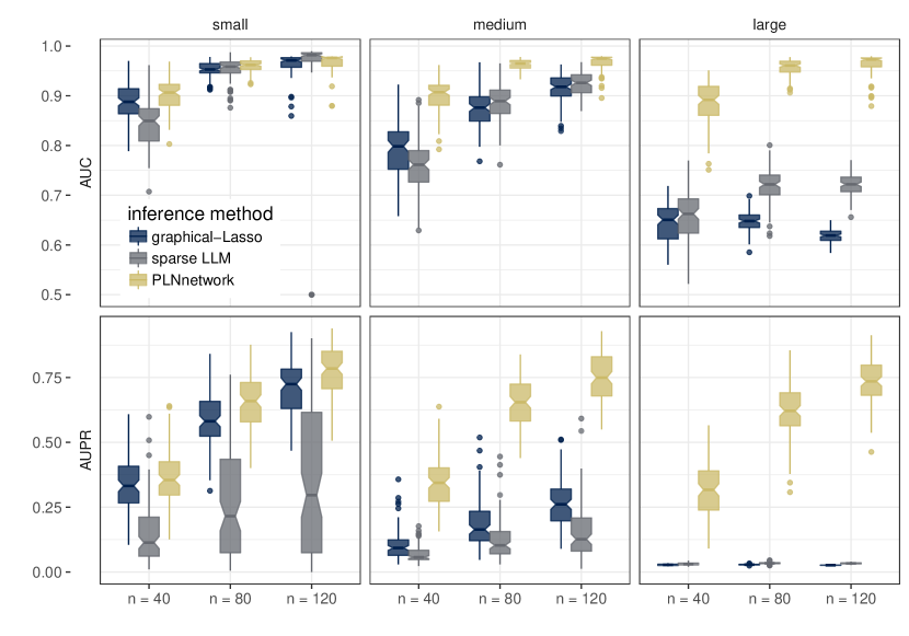
Figure 3: Effect of the variability of the sampling effort, a.k.a the compositional problem, on the quality of the reconstruction of 50-node random networks. First and second row respectively represent AUC and AUPR boxplots computed on 100 simulations.

Accounting for covariates effect does matter.

We now focus on the effect of an external covariate in the data, and how it affects the performance of the methods. Regarding the sampling effort, we fix $\nu=2$ in this experiment, and we only compare the compositional methods together since the other approaches would fail in this setting. The strength of the covariate effect is controlled by the parameter $b$ in our compositional model. The larger $b$, the larger the effect of the covariate and the harder the problem of network reconstruction when not accounting for the covariate. We vary $b\in\{1,2,3\}$, hence, a small, medium and large effect. On top of that, we vary the sample size and consider the three network topologies (scale-free, random and community networks), always with $p=50$ nodes. We evaluate the performance of SPiEC-Easi, sparCC and PLNnetwork in terms of AUC and AUPR on 100 simulation of each kind and report the average values in Table 1.

		area under the ROC						area under the PR
covar.	method	$\mathbf{n=p/2}$		$\mathbf{n=p}$		$\mathbf{n=2p}$		$\mathbf{n=p/2}$		$\mathbf{n=p}$		$\mathbf{n=2p}$
scale-free network
small	PLNnetwork	.66 (	0.05)	.78 (	0.05)	.91 (	0.03)	.11 (	0.04)	.25 (	0.07)	.49 (	0.08)
	sparCC	.66 (	0.05)	.73 (	0.05)	.79 (	0.05)	.09 (	0.03)	.16 (	0.05)	.24 (	0.07)
	SPiEC-Easi	.67 (	0.04)	.77 (	0.05)	.85 (	0.04)	.10 (	0.03)	.17 (	0.05)	.27 (	0.07)
medium	PLNnetwork	.62 (	0.05)	.73 (	0.05)	.85 (	0.05)	.09 (	0.03)	.18 (	0.06)	.34 (	0.08)
	sparCC	.55 (	0.05)	.57 (	0.05)	.58 (	0.05)	.05 (	0.01)	.05 (	0.01)	.06 (	0.01)
	SPiEC-Easi	.61 (	0.04)	.66 (	0.04)	.71 (	0.03)	.06 (	0.01)	.06 (	0.01)	.07 (	0.01)
large	PLNnetwork	.58 (	0.05)	.67 (	0.05)	.78 (	0.05)	.07 (	0.03)	.12 (	0.04)	.23 (	0.07)
	sparCC	.52 (	0.04)	.53 (	0.04)	.53 (	0.05)	.04 (	0.01)	.04 (	0.01)	.04 (	0.01)
	SPiEC-Easi	.57 (	0.04)	.60 (	0.03)	.65 (	0.03)	.05 (	0.01)	.05 (	0.01)	.05 (	0.01)
random network
small	PLNnetwork	.77 (	0.07)	.90 (	0.04)	.96 (	0.01)	.14 (	0.07)	.36 (	0.11)	.64 (	0.09)
	sparCC	.76 (	0.06)	.83 (	0.06)	.89 (	0.04)	.11 (	0.05)	.23 (	0.09)	.36 (	0.11)
	SPiEC-Easi	.78 (	0.05)	.87 (	0.04)	.92 (	0.03)	.11 (	0.05)	.23 (	0.09)	.36 (	0.11)
medium	PLNnetwork	.72 (	0.06)	.85 (	0.05)	.94 (	0.02)	.09 (	0.04)	.24 (	0.09)	.49 (	0.10)
	sparCC	.59 (	0.06)	.61 (	0.07)	.62 (	0.06)	.03 (	0.01)	.04 (	0.02)	.04 (	0.02)
	SPiEC-Easi	.67 (	0.05)	.74 (	0.05)	.77 (	0.03)	.04 (	0.01)	.05 (	0.02)	.05 (	0.01)
large	PLNnetwork	.64 (	0.07)	.78 (	0.06)	.88 (	0.04)	.06 (	0.03)	.14 (	0.07)	.29 (	0.09)
	sparCC	.54 (	0.05)	.53 (	0.06)	.54 (	0.06)	.02 (	0.01)	.02 (	0.01)	.03 (	0.01)
	SPiEC-Easi	.61 (	0.05)	.65 (	0.04)	.68 (	0.03)	.03 (	0.00)	.03 (	0.00)	.03 (	0.01)
community network
small	PLNnetwork	.60 (	0.04)	.69 (	0.04)	.78 (	0.05)	.17 (	0.03)	.26 (	0.04)	.38 (	0.05)
	sparCC	.62 (	0.04)	.66 (	0.04)	.70 (	0.04)	.16 (	0.02)	.21 (	0.04)	.26 (	0.04)
	SPiEC-Easi	.62 (	0.04)	.70 (	0.04)	.77 (	0.04)	.17 (	0.02)	.24 (	0.04)	.31 (	0.04)
medium	PLNnetwork	.57 (	0.03)	.65 (	0.04)	.73 (	0.05)	.15 (	0.02)	.22 (	0.03)	.31 (	0.05)
	sparCC	.55 (	0.03)	.56 (	0.04)	.56 (	0.03)	.11 (	0.02)	.12 (	0.02)	.12 (	0.02)
	SPiEC-Easi	.58 (	0.03)	.63 (	0.03)	.67 (	0.03)	.13 (	0.02)	.14 (	0.02)	.15 (	0.02)
large	PLNnetwork	.55 (	0.03)	.60 (	0.04)	.67 (	0.04)	.13 (	0.02)	.17 (	0.03)	.24 (	0.04)
	sparCC	.52 (	0.03)	.52 (	0.03)	.52 (	0.03)	.10 (	0.02)	.10 (	0.02)	.10 (	0.02)
	SPiEC-Easi	.55 (	0.03)	.58 (	0.03)	.62 (	0.03)	.11 (	0.01)	.11 (	0.02)	.12 (	0.01)

Table 1: Areas under the ROC curve and Areas under the Precision-Recall curve of the compositional methods (PLNnetwork, sparCC and SPiEC-Easi) in various settings, averaged over 100 simulations, with standard errors.

PLNnetwork, which is the only method that can effectively account for the covariate effect, is a clear leader in almost all settings. Even when the effect of the covariate is small, it seems to outperform its competitors, except in the high dimensional setup and for community network, where all methods perform similarly. We underline that the superiority of PLNnetwork is even clearer in terms of AUPR. In other words, PLNnetwork – as a statistical method – has a similar or higher power than its competitors while keeping a lower false positive rate.

Model Selection issue.

In this numerical study, we focus on PLNnetwork and address the difficult question of choosing the tuning parameter and compare the two alternatives presented in Section 3. Figure 4 reports the results of our numerical experiments on model selection: we compare the StARS criterion computed on 50 subsamples with a stability threshold of $1-2\beta=0.95$ as recommended by Liu et al., to the BIC for choosing $\lambda$ in PLNnetwork. We give the performance in terms of precision/recall and fall-out/recall averaged over 100 simulation, which correspond to single points on the PR and ROC curves respectively. As can been seen, StARS systematically outperforms BIC in terms of recall and precision. However, this increase in performance comes at a huge computational burden.

	choice on ROC curve		choice on PR curve
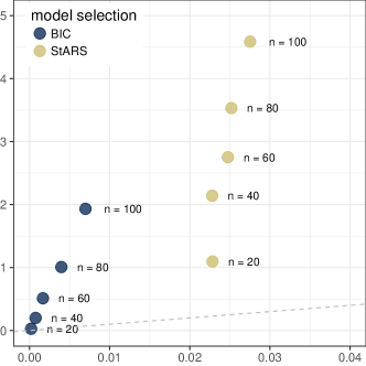
recall		precision
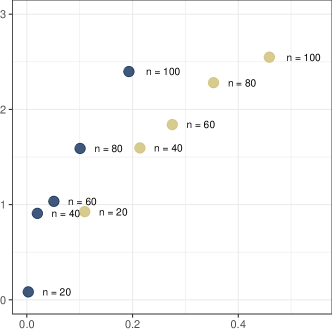
	fall-out		recall

Figure 4: Performance of the model selection procedures (BIC or StARS) in PLNnetwork for reconstructing 50-node randoms networks, averaged over 100 simulations.

5 Illustrations

We now illustrate our methodology with a series of examples from different fields. Barents fish is a simple ecological example that we use to emphasizes the importance of accounting for covariates when performing structure inference. The French election example shows that our method can handle large datasets; we also use it to show how to interpret the results and propose some validation checks. Finally we consider a metagenomic example (Oak mildew), for which we propose a deeper analysis. More specifically, we show how to decompose the effects of the different covariates on the inferred interactions and we propose some biological interpretations of the results.

5.1 Barents fish

The data consist in the abundance of $p=30$ fish species measured in $n=89$ stations from the Barents sea between April and May 1997. The data have been collected and described by Fossheim et al. (2006) and re-analyzed by Greenacre (2013); Greenacre and Primicerio (2014). For each sample, the latitude and longitude of the station as well as the temperature and depth were recorded. Thanks to a precise experimental protocol, all abundances are comparable so no offset term is required in the model. Our aim here is to illustrate how the inclusion of covariates avoids spurious edges in the inferred network.

Introducing covariates reduces the number of inferred edges.

To this aim, we fitted the PLN-network model with ($a$) no covariates, ($b$) two environmental covariates (temperature and depth) and ($c$) all covariates (i.e. the previous two and geographical location) using the same penalty grid every time with $\lambda$ increasing geometrically from $0.03$ to $15.17$. As expected, Figure 5 (top right panel) shows that, for all models, the number of edges increases as the penalty decreases. It also shows that, for any penalty, the number of edges decreases as (plain lines) the richness of the model increases ($c>b>a$) and that most edges recovered in the full ($c$) model are also recovered in the partial models ($a$, black dotted curve) and ($b$, blue dotted curve). This suggests that naive inference is likely to find not only genuine edges but also spurious ones corresponding to co-variations induced by external covariates. Interestingly, the dotted curve shows that the proportion of common edges between models $b$ and $c$ is higher than the one between models $a$ and $c$. This suggests that environmental covariates explain a substantial part of the apparent species co-variations.

Spurious interactions can be linked with specific covariates.

The rest of Figure 5 displays the networks inferred with the three models for three different levels of sparsity (controlled by $\lambda$). For an illustrative purpose, the values of $\lambda$ have been chosen so that, in average, each species interacts with two others for each of the three models ($a$), ($b$) and ($c$). This results in networks with approximately $2p=60$ edges. The comparison of these networks confirms the conclusions obtained in the simulation study. One additional conclusion is that a set of core species seem to have direct interactions, or at least, interactions that cannot be simply explained by geographical location and environmental covariates (bottom right panel).

On the contrary, some interactions seem to be actually indirect. For example, the interactions between the longear eelpout (Ly.se) and some species from the core group disappear when accounting for temperature and depth, suggesting that the covariation of their respective abundances results from variations of the environmental conditions. Similarly, the interactions between the Greenland halibut (Re.hi) and the core group is kept when introducing temperature and depth in the model, but disappears when accounting for location (longitude and latitude) suggesting that these interactions actually reflect a common response to fluctuations of biotic and abiotic characteristics across sites.

To confirm this interpretation, we fitted an over-dispersed Poisson generalized linear model for the abundance of both species (not shown). We found that both temperature and depth have a significant effect on the abundance of the longear eelpout and that the longitude has a significant influence on the abundance of the Greenland halibut (all corresponding $p$-values being smaller than $1e^{-4}$).

	($a$) no covariate	($b$) temperature & depth	($c$) all covariates
$\lambda=.84$
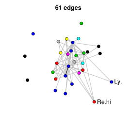
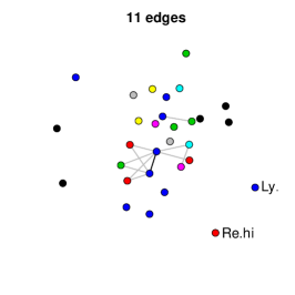
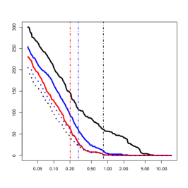
$\lambda=.28$
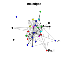
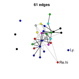
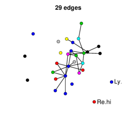
$\lambda=.20$

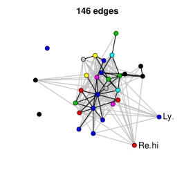
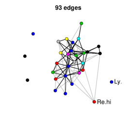
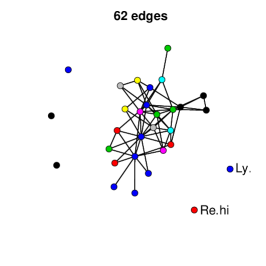
Figure 5: Inferred networks with increasing penalties (top: $\lambda=.84$, middle: $\lambda=.28$, bottom: $\lambda=.20$) for different covariate sets (see top line). Each node corresponds to a given species. The position of the nodes are kept fixed. Node color: species family (see Fossheim et al., 2006). Black edges: edges in common with the network inferred with all covariates and same $\lambda$. The missing network (top right panel, all covariates and $\lambda=.84$) contains only one edge. Top right: number of edges as a function of $\lambda$. Black: no covariate, blue: temperature and depth, red: all covariates, dotted black: common edges with no and all covariates, dotted blue: common edges between two and all covariates. Vertical dashed lines: the three chosen values of $\lambda$.

5.2 French Presidential Elections, 2017

Our second dataset comes from the first round of the French presidential election of 2017 and consists in the votes cast for each of the 11 candidates in the more than 63 000 polling stations. Our goal here is to find competing candidates, who appeal to different voters, and compatible candidates, who appeal to the same voters, after accounting for the fact that elections are a zero-sum game.

Data were downloaded from the French open data platform data.gouv.fr and filtered to remove stations with no votes. To reduce inference times, we consider a random subset of 13,704 stations that accounted for 20% of the registered population. The voting population in those booths varied wildly, ranging from 10 to 105,891 (6th district of French citizens living abroad) registered voters, with a median at 736 and 99.5% of the stations with less than 1,700 voters. We consider the log-registered population of voters, and not log-turnout, as an offset to account for different station sizes. This means in particular that votes are not affected by the compositionality effect as much as in other settings, as they do not sum up to the offset. Voting patterns are well-known to depend on geography and we therefore consider department (a French administrative division) as a proxy for geography.

We consider three models in total: without offset, with offset but no covariate, with offset and covariates and use the same grid of $\lambda$ – decreasing geometrically from 1 to $1e^{-3}$ in 31 steps – for all. The optimal value $\lambda^{\star}$ was selected using StARS with 100 subsamples of size 1170 ($\simeq 10\sqrt{n}$). Results of our analysis are displayed in Figure 6.

	No offset	Offset	Offset + Departments
Networks
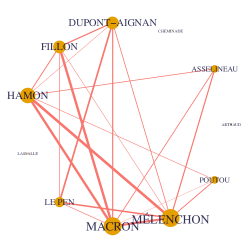
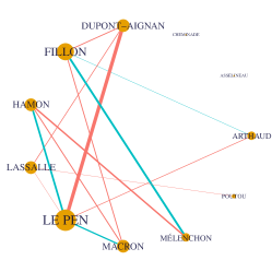
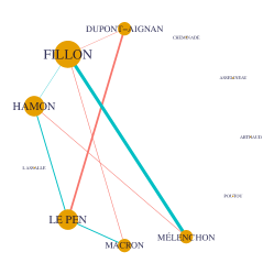
Latent Positions $\mathbf{M}$ (PCA)

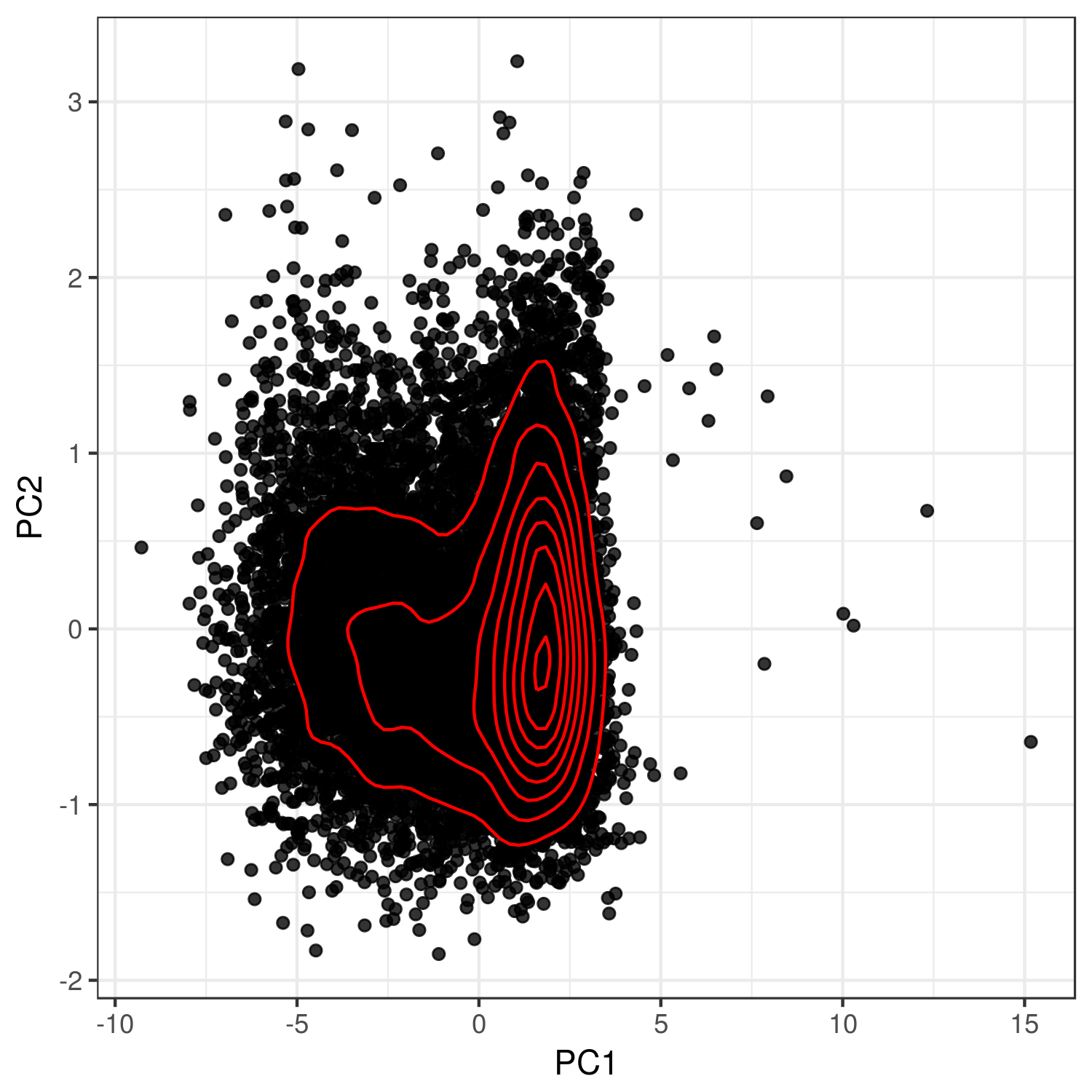
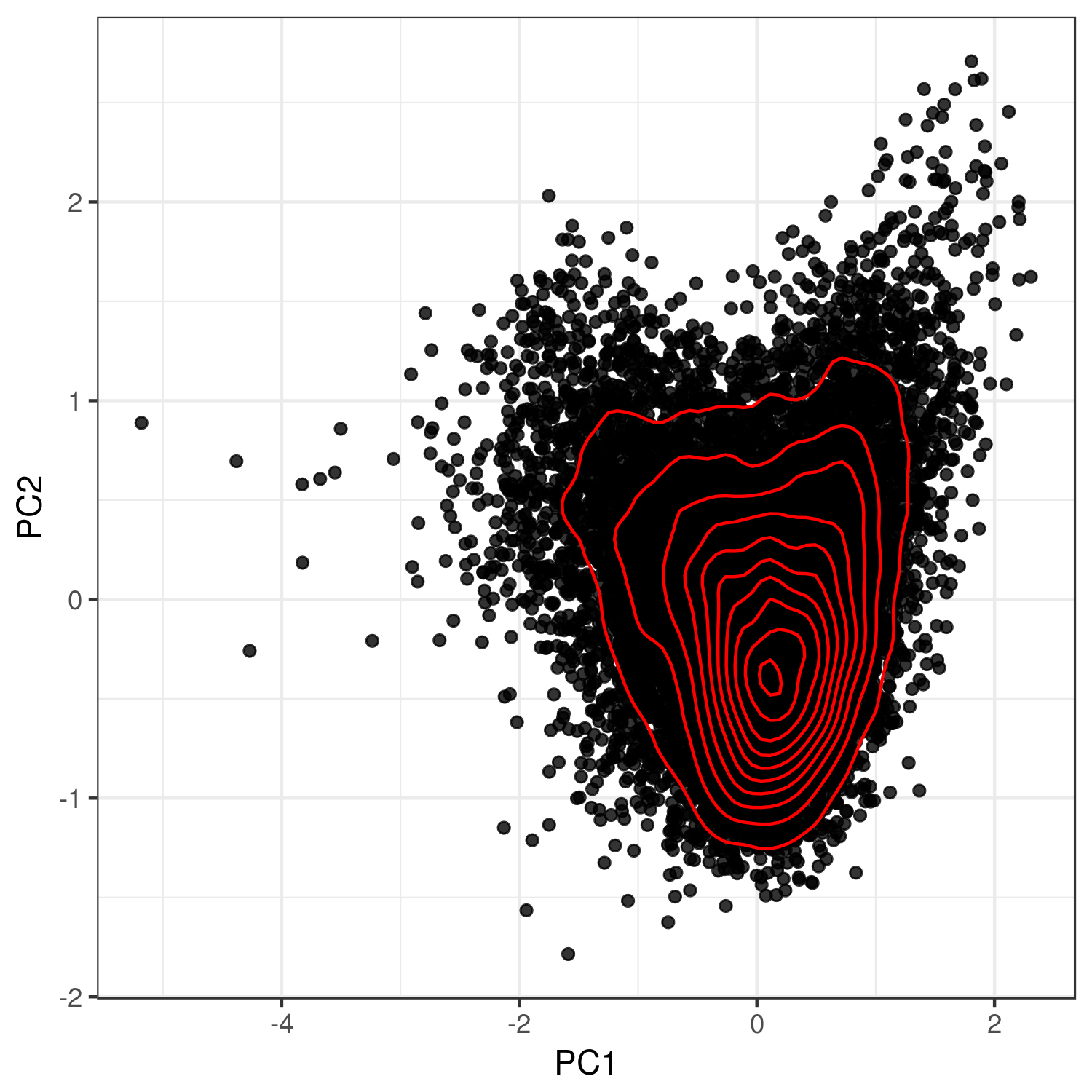
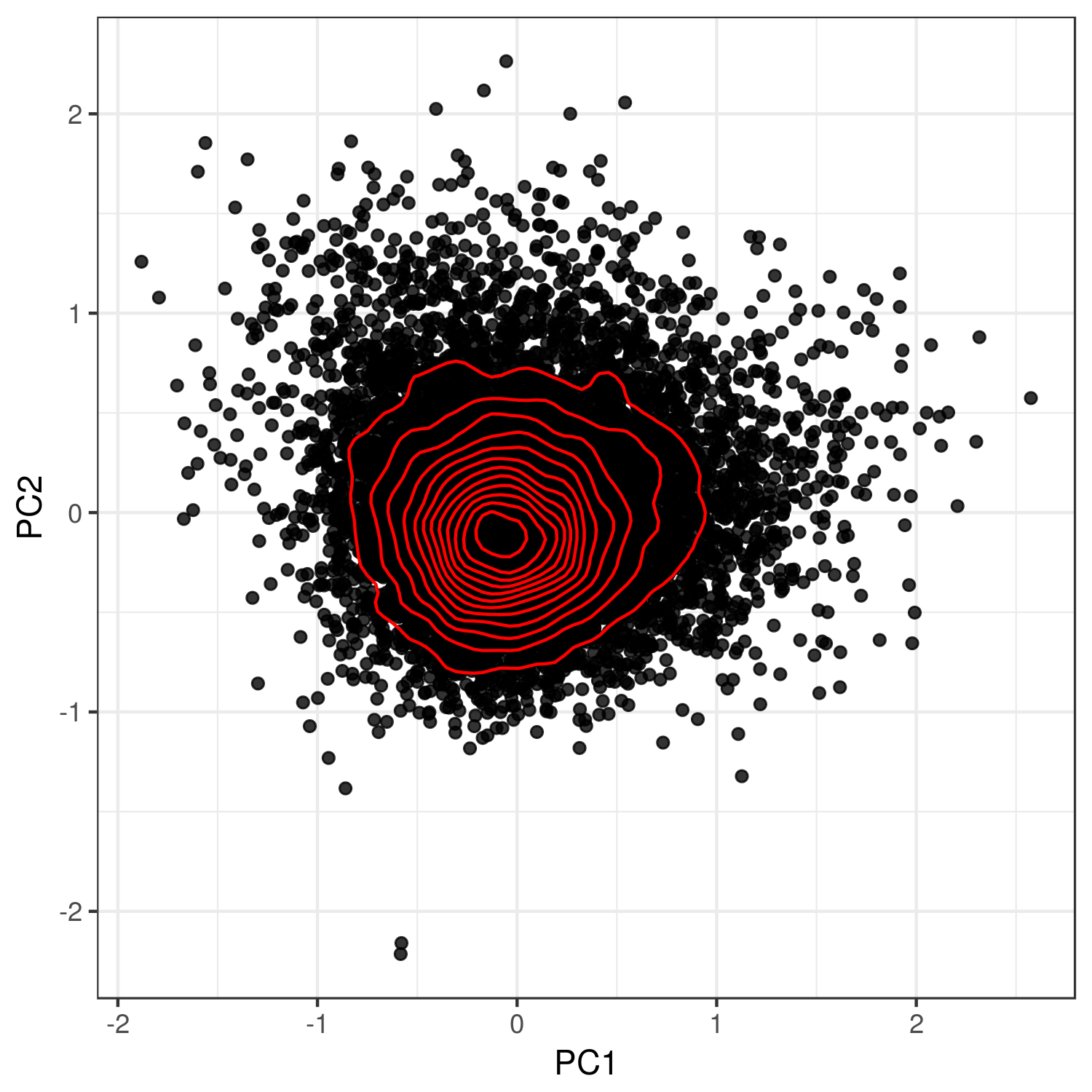
Figure 6: Network between candidates of last French presidential elections. Top row: Networks inferred under different models. Edges represent partial correlations $\rho_{ij}$: their thickness is proportional to $|\rho_{ij}|$ and they are colored red if $\rho_{ij}>0$ and blue if $\rho_{ij}<0$. A node’s size and label size are proportional to its degree. Bottom row: Positions $\mathbf{M}$ of the polling stations in the Gaussian latent space. Since the latent space has dimension $11$, we performed a PCA of $\mathbf{M}$ and show only the principal plane. Red lines represent contour lines of the density estimated with a 2D kernel. The density should be bivariate Gaussian and departures from elliptic curves reveal remaining structure not accounted for in the model.

The offset matters.

Figure 6 shows that the inclusion of an offset drastically reduces the density of the reconstructed network and alters the sign and strength of partial correlations. Failing to accoung for varying station sizes leads to a spurious positive partial correlations between most candidates: the shift of all stations towards the positive orthant in the latent space are mistaken for positive correlations between all coordinates. The offset counteracts this by translating back all stations towards the origin along the direction $\mathbb{R}\mathbf{1}$.

Correcting for geography is important.

Figure 6 also shows that correcting for geography also changes the graph but to a lesser extent. However, when we move back to the Gaussian latent space and examine the latent positions of the polling stations ($\mathbf{M}$), we do not observe the expected elliptic distribution of a multivariate Gaussian (Fig. 6, left panel). Taking the department of origin into account helps recover ellipticity and confirms that geography is indeed a strong structuring factor in the latent space.

Political interactions.

If we consider the network reconstructed with the offset and geographic covariate as the most reliable, results show that candidate with similar political leaning appeal to the same voters (M. Le Pen and N. Dupont-Aignan (both far right), B. Hamon (left) and J.-L. Mélenchon (far left), E. Macron (center) and J.-F. Fillon (right)) whereas candidate with different leanings appeal to different voters (M. Le Pen versus B. Hamon and E. Macron, J.-F. Fillon versus J.-L. Mélenchon). More precisely, a negative partial correlation between candidates A and B means, all other things being equal, that a high vote for one candidate in a station is correlated to a low vote for the other.

This may explain the absence of negative correlation between far left and far right: although their electorates may differ, they vote in the same stations. Similarly, the fact that the positive partial correlation between E. Macron and B. Hamon disappears when controlling for geography means that they have high voter shares in the same departments but not necessarily in the same polling stations. This is confirmed by the high correlation ($0.76$) of their respective regression coefficients across departments.

5.3 Oak mildew

The metagenomic dataset introduced in Jakuschkin et al. (2016) consists of microbial communities sampled on the surface of oak leaves (the samples). The leaves were collected on trees with different resistance levels to the fungal pathogenic species E. alphitoides, responsible for the oak powdery mildew. Table 2 provides the available classification information about the bacterial and fungal OTU appearing in at least one network inferred in our analysis. Unfortunately, not all OTU can been identified at the species level and some OTU are not related to any known species. In the following, we consider two groups of samples labeled by Jakuschkin et al.: $n_{r}=39$ resistant samples (where E. alphitoides was essentially absent) and $n_{s}=39$ susceptible samples (where a significant activity of E. alphitoides was detected). In addition to the sampling tree, several covariates, all thought to potentially structure the community, were measured for each leaf: orientation, distance to trunk, distance to ground, distance to base. After sequencing, clustering into operating taxononomic units (or OTU – a proxy for species), and a final filtering of the identified bacterial and fungal communities with too few reads, the total number of species considered is $p=114$ OTUs in this data set (66 bacterial ones and 48 fungal ones, including E. alphitoides).

Type	OTU	Family	Genus	Species
Fungi	f1	Dermateaceae	Naevala	Naevala minutissima
	f3	–	–	–
	f4	Erysiphaceae	Erysiphe	Erysiphe hypophylla
	f8	Hyaloscyphaceae	Catenulifera	Catenulifera brevicollaris
	f10	–	–	–
	f12	Amphisphaeriaceae	Monochaetia	Monochaetia kansensis
	f17	Herpotrichiellaceae	Cyphellophora	Cyphellophora hylomeconis
	f19	–	–	–
	f25	unidentified	Cryptococcus	Cryptococcus magnus
	f27	unidentified	Strelitziana	Strelitziana mali
	f29	Mycosphaerellaceae	Xenosonderhenia	Xenosonderhenia syzygii
	f32	–	–	–
	f39	–	–	–
	f1085	Mycosphaerellaceae	Mycosphaerella	Mycosphaerella marksii
	f1090	Herpotrichiellaceae	Cyphellophora	Cyphellophora hylomeconis
	f1278	Mycosphaerellaceae	Mycosphaerella	Mycosphaerella punctiformis
	Ea	Erysiphaceae	Erysiphe	Erysiphe alphitoides
Bacteria	b13	Oxalobacteraceae	–	–
	b153	Oxalobacteraceae	–	–
	b21	Pseudomonadaceae	Pseudomonas	–
	b25	Enterobacteriaceae	–	–
	b26	Oxalobacteraceae	–	–
	b33	Microbacteriaceae	Rathayibacter	–
	b364	Oxalobacteraceae	–	–
	b37	Beijerinckiaceae	Beijerinckia	–
	b44	–	–	–
	b60	–	–	–

Table 2: Type of microorganism (bacteria or fungi) and higher level taxonomic assignments (family, genus and species) of the 27 operational taxonomic units (OTUs) interacting in the inferred microbial networks. Unknown assignments at a given rank are reported as ’–’.

Our aim here is to unravel the association between the different microbial and fungal species by reconstructing the ecological network. Obviously, we are especially interested in the interactions between E. alphitoides and the other species. We emphasize that unlike SPiEC-Easi or sparCC, that are limited to interactions between bacteria or between fungi due their normalisation step, we can actually investigate interactions between bacterial and fungi E. alphitoides although the sequencing depths differ for each type. A similar target was already at the core of Jakuschkin et al.’s work. However our approach differs from a methodological view-point as we jointly estimate the effect of the covariates $\mathbf{B}$ and the dependency structure $\mathbf{\Omega}$ while they only corrected the observed counts for the effect of the covariates using a regression model before feeding the residuals from that regression to a network inference method. This two-steps procedure fails to account for the fact that $\mathbf{B}$ is estimated and to propagate uncertainty from the first step to the second one. Moreover, Jakuschkin et al. focused their study on the set of susceptible samples, while we propose here to infer three networks: one for susceptible samples, one for resistant samples and one for merged samples. By these means, we hope to obtain a more thorough map of interactions between the pathogen and its ecosystem.

The three PLN models respectively including the susceptible, the resistant and both samples were defined as follows: for the susceptible and the resistant models, we applied PLNnetwork by including simple effects of the orientation and of the distance to the trunk (the distances to the ground and to the base were highly correlated with the former, and we used it as a representative of these three covariates). For the model merging all the samples, we added the covariate describing the tree status (either resistant or susceptible), with both simple effects and interactions with the two other covariates (orientation and distance to trunk). These two approaches – separating or merging the samples – address different yet complementary goals: by separating the samples, we assume that the two underlying networks (and thus covariances) are different and need a specific analysis; the counterpart that merges all samples aims to render a synergistic network that encompasses important interactions from both situations after correction of the mean effects due to the tree status (resistant or susceptible).

resistant samples	susceptible samples
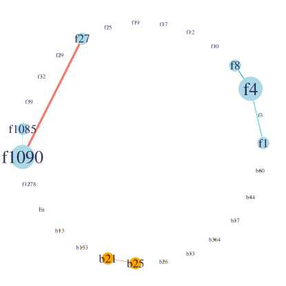
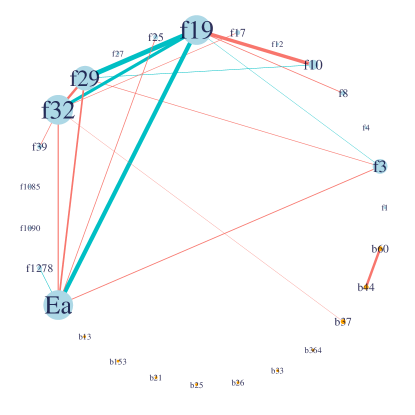
samples from both origins	regression coefficient for orientation

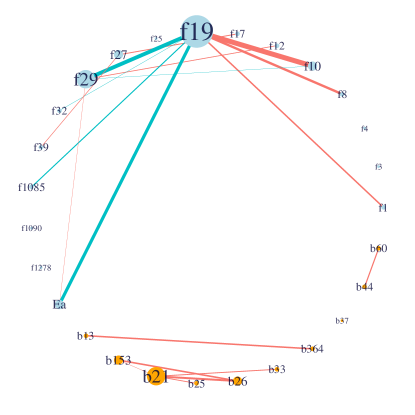
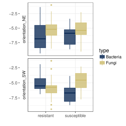
Figure 7: Oak mildew network analysis: networks inferred by PLNnetwork and selected by StARS for a stability of $0.995$. Each network correspond to networks inferred using samples respectively from the resistant tree, the susceptible tree and when merging samples from both origins. Blue vertices represent Fungi; orange vertices represent bacteria. Edges represent partial correlations $\rho_{ij}$: edge thickness is proportional to $|\rho_{ij}|$ and are colored red if $\rho_{ij}>0$ and blue if $\rho_{ij}<0$. A node’s size and label size are proportional to its degree. Only nodes having at least one edge among the three networks are included in the plots. Inset: Boxplot of regression coefficient of abundances against orientation.

Before getting into the interpretation of the results in terms of species interactions, we remind that the PLN models also enables to measure the effect of the covariates on each species. The bottom right panel of Figure 7 displays the distribution of the regression parameters of the two orientation indicators (NE $=$ north-east and SW $=$ south-west), in each tree, across each species type. We do not discuss extensively these results but one may observe a strong interaction between SW orientation and tree type on both fungi and bacteria: bacteria are notably depleted in leaves facing SW in susceptible trees.

We now focus on the results of our analysis in terms of networks in Figure 7. All networks inferred with PLNnetwork where selected with StARS on a 50-size grid of penalties, using a high stability level of $1-2\beta=0.995$ to drastically limit the number of false positive edges. The top row displays the resistant and susceptible networks, showing very different patterns, while the consensus network seems to catch features from both of them. In the susceptible network, E. alphitoides is identified as ($i$) antagonist to fungi f1278, from the Mycosphaerella punctiformis species, which colonizes living oak leaves asymptomatically and may prevent infection by E. alphitoides and ($ii$) mutualist to fungi f29, from the Xenosonderhenia syzygii species, usually found in leaf spots, common on weakened and senescent leaves. The other mutualists of E. alphitoides unfortunately belong to unknown species and no similar observations can be made. Interestingly, in the susceptible network, the pathogen has less interactions than fungi f19, but is connected to it, whereas both have few connections in the resistant network. As E. alphitoides is known to be responsible for the mildew disease, the comparison of these networks suggest that its pathogenic effect is partially mediated by f19. In addition to the direct effect of the pathogen on a small set of species, its (negative) effect on fungi f19, which seems to play a central role in the phyllosphere, leverages its impact on the whole system. Finally, the consensus network encompassing both sources of samples resembles the susceptible network, with some notable discrepancies: a cluster composed by bacterial species b21, b25, b26, b153 and to a lesser extent b33 is found in the consensus network, which was only incipient in the resistant network. This is probably due to the gain in power induced by a larger sample-size.

Acknowledgement

We thank Charlie Pauvert for beta-testing our implementation and for his feedback. This work was funded by projects LearnBioControl, Brassica-Dev from the Inra MEM metaprogramme.

References

- Agresti (1996) A. Agresti. An introduction to categorical data analysis, volume 135. Wiley New York, 1996.
- Aitchison and Ho (1989) J. Aitchison and C. Ho. The multivariate poisson-log normal distribution. Biometrika, 76(4):643–653, 1989.
- Allen and Liu (2012) G. I. Allen and Z. Liu. A log-linear graphical model for inferring genetic networks from high-throughput sequencing data. In Bioinformatics and Biomedicine (BIBM), 2012 IEEE International Conference on, pages 1–6. IEEE, 2012.
- Banerjee et al. (2008) O. Banerjee, L. E. Ghaoui, and A. d’Aspremont. Model selection through sparse maximum likelihood estimation for multivariate gaussian or binary data. Journal of Machine learning research, 9(Mar):485–516, 2008.
- Besag (1974) J. Besag. Spatial interaction and the statistical analysis of lattice systems. Journal of the Royal Statistical Society. Series B (Methodological), pages 192–236, 1974.
- Biswas et al. (2016) S. Biswas, M. Mcdonald, D. S. Lundberg, J. L. Dangl, and V. Jojic. Learning microbial interaction networks from metagenomic count data. Journal of Computational Biology, 23(6):526–535, 2016. doi: https://doi.org/10.1089/cmb.2016.0061. URL http://online.liebertpub.com/doi/10.1089/cmb.2016.0061.
- Cai et al. (2011) T. Cai, W. Liu, and X. Luo. A constrained 1 minimization approach to sparse precision matrix estimation. Journal of the American Statistical Association, 106(494):594–607, 2011.
- Chandrasekaran et al. (2012) V. Chandrasekaran, P. A. Parrilo, and A. S. Willsky. Latent variable graphical model selection via convex optimization. The Annals of Statistics, 40(4):1935–1967, 2012.
- Chen and Chen (2008) J. Chen and Z. Chen. Extended bayesian information criteria for model selection with large model spaces. Biometrika, 95(3):759–771, 2008.
- Chib and Greenberg (1995) S. Chib and E. Greenberg. Understanding the metropolis-hastings algorithm. The American Statistician, 49(4):327–335, 1995.
- Chiquet et al. (to appear) J. Chiquet, M. Mariadassous, and S. Robin. Variational inference for probabilistic poisson pca. Ann. Appl. Statist., to appear.
- Davis and Goadrich (2006) J. Davis and M. Goadrich. The relationship between precision-recall and roc curves. In Proceedings of the 23rd international conference on Machine learning, pages 233–240. ACM, 2006.
- Dempster et al. (1977) A. P. Dempster, N. M. Laird, and D. B. Rubin. Maximum likelihood from incomplete data via the EM algorithm. J. R. Statist. Soc. B, 39:1–38, 1977.
- Drew et al. (2017) K. Drew, C. L. Müller, R. Bonneau, and E. M. Marcotte. Identifying direct contacts between protein complex subunits from their conditional dependence in proteomics datasets. PLOS Computational Biology, 13(10):1–23, 10 2017. doi: 10.1371/journal.pcbi.1005625. URL https://doi.org/10.1371/journal.pcbi.1005625.
- Fiers et al. (2018) M. W. E. J. Fiers, L. Minnoye, S. Aibar, C. Bravo González-Blas, Z. Kalender Atak, and S. Aerts. Mapping gene regulatory networks from single-cell omics data. Briefings in Functional Genomics, page elx046, 2018. doi: 10.1093/bfgp/elx046. URL http://dx.doi.org/10.1093/bfgp/elx046.
- Fossheim et al. (2006) M. Fossheim, E. M. Nilssen, and M. Aschan. Fish assemblages in the barents sea. Marine Biology Research, 2(4):260–269, 2006.
- Foygel and Drton (2010) R. Foygel and M. Drton. Extended bayesian information criteria for gaussian graphical models. In Advances in neural information processing systems, pages 604–612, 2010.
- Friedman and Alm (2012) J. Friedman and E. J. Alm. Inferring correlation networks from genomic survey data. PLOS Computational Biology, 8(9):1–11, 09 2012. doi: 10.1371/journal.pcbi.1002687. URL http://dx.doi.org/10.1371%2Fjournal.pcbi.1002687.
- Friedman et al. (2008) J. Friedman, T. Hastie, and R. Tibshirani. Sparse inverse covariance estimation with the graphical lasso. Biostatistics, 9(3):432–441, 2008.
- Gallopin et al. (2013) M. Gallopin, A. Rau, and F. Jaffrézic. A hierarchical poisson log-normal model for network inference from rna sequencing data. PLOS ONE, 8(10):1–9, 10 2013. doi: 10.1371/journal.pone.0077503. URL https://doi.org/10.1371/journal.pone.0077503.
- Greenacre (2013) M. Greenacre. Fuzzy coding in constrained ordinations. Ecology, 94(2):280–286, 2013.
- Greenacre and Primicerio (2014) M. Greenacre and R. Primicerio. Multivariate analysis of ecological data. Fundacion BBVA, 2014.
- Harris (2016) D. J. Harris. Inferring species interactions from co-occurrence data with markov networks. Ecology, 97(12):3308–3314, 2016. ISSN 1939-9170. doi: 10.1002/ecy.1605. URL http://dx.doi.org/10.1002/ecy.1605.
- Imbert et al. (2017) A. Imbert, A. Valsesia, C. Le Gall, C. Armenise, G. Lefebvre, P.-A. Gourraud, N. Viguerie, and N. Villa-Vialaneix. Multiple hot-deck imputation for network inference from rna sequencing data. Bioinformatics, page btx819, 2017.
- Inouye et al. (2017) D. I. Inouye, E. Yang, G. I. Allen, and P. Ravikumar. A review of multivariate distributions for count data derived from the poisson distribution. Wiley Interdisciplinary Reviews: Computational Statistics, 9(3), 2017.
- Jakuschkin et al. (2016) B. Jakuschkin, V. Fievet, L. Schwaller, T. Fort, C. Robin, and C. Vacher. Deciphering the pathobiome: Intra-and interkingdom interactions involving the pathogen Erysiphe alphitoides. Microbial ecology, pages 1–11, 2016.
- Johnson (2011) S. G. Johnson. The NLopt nonlinear-optimization package, 2011. URL http://ab-initio.mit.edu/nlopt.
- Karlis (2005) D. Karlis. EM algorithm for mixed Poisson and other discrete distributions. Astin bulletin, 35(01):3–24, 2005.
- Khare et al. (2015) K. Khare, S.-Y. Oh, and B. Rajaratnam. A convex pseudolikelihood framework for high dimensional partial correlation estimation with convergence guarantees. Journal of the Royal Statistical Society: Series B (Statistical Methodology), 77(4):803–825, 2015.
- Kurtz et al. (2015) Z. D. Kurtz, C. L. Müller, E. R. Miraldi, D. R. Littman, M. J. Blaser, and R. A. Bonneau. Sparse and compositionally robust inference of microbial ecological networks. PLoS Comput Biol, 11(5):e1004226, May 2015. doi: 10.1371/journal.pcbi.1004226. URL http://dx.doi.org/10.1371/journal.pcbi.1004226.
- Lauritzen (1996) S. L. Lauritzen. Graphical Models. Oxford Statistical Science Series. Clarendon Press, 1996.
- Lima-Mendez et al. (2015) G. Lima-Mendez, K. Faust, N. Henry, J. Decelle, S. Colin, F. Carcillo, S. Chaffron, J. C. Ignacio-Espinosa, S. Roux, F. Vincent, L. Bittner, Y. Darzi, J. Wang, S. Audic, L. Berline, G. Bontempi, A. M. Cabello, L. Coppola, F. M. Cornejo-Castillo, F. d’Ovidio, L. De Meester, I. Ferrera, M.-J. Garet-Delmas, L. Guidi, E. Lara, S. Pesant, M. Royo-Llonch, G. Salazar, P. Sánchez, M. Sebastian, C. Souffreau, C. Dimier, M. Picheral, S. Searson, S. Kandels-Lewis, G. Gorsky, F. Not, H. Ogata, S. Speich, L. Stemmann, J. Weissenbach, P. Wincker, S. G. Acinas, S. Sunagawa, P. Bork, M. B. Sullivan, E. Karsenti, C. Bowler, C. de Vargas, and J. Raes. Determinants of community structure in the global plankton interactome. Science, 348(6237), 2015. ISSN 0036-8075. doi: 10.1126/science.1262073. URL http://science.sciencemag.org/content/348/6237/1262073.
- Liu et al. (2009) H. Liu, J. Lafferty, and L. Wasserman. The nonparanormal: Semiparametric estimation of high dimensional undirected graphs. Journal of Machine Learning Research, 10(Oct):2295–2328, 2009.
- Liu et al. (2010a) H. Liu, K. Roeder, and L. Wasserman. Stability approach to regularization selection (stars) for high dimensional graphical models. In Proceedings of the 23rd International Conference on Neural Information Processing Systems - Volume 2, NIPS’10, pages 1432–1440, USA, 2010a. Curran Associates Inc. URL http://dl.acm.org/citation.cfm?id=2997046.2997056.
- Liu et al. (2010b) H. Liu, K. Roeder, and L. Wasserman. Stability approach to regularization selection (stars) for high dimensional graphical models. In Advances in neural information processing systems, pages 1432–1440, 2010b.
- Ma et al. (2008) J. Ma, K. M. Kockelman, and P. Damien. A multivariate poisson-lognormal regression model for prediction of crash counts by severity, using bayesian methods. Accident Analysis & Prevention, 40(3):964–975, 2008.
- Meinshausen and Bühlmann (2006) N. Meinshausen and P. Bühlmann. High-dimensional graphs and variable selection with the lasso. Ann. Statist., 34(3):1436–1462, 06 2006. doi: 10.1214/009053606000000281. URL https://doi.org/10.1214/009053606000000281.
- Moignard et al. (2015) V. Moignard, S. Woodhouse, L. Haghverdi, A. J. Lilly, Y. Tanaka, A. C. Wilkinson, F. Buettner, I. C. Macaulay, W. Jawaid, E. Diamanti, et al. Decoding the regulatory network of early blood development from single-cell gene expression measurements. Nature biotechnology, 33(3):269, 2015.
- Park and Lord (2007) E. Park and D. Lord. Multivariate poisson-lognormal models for jointly modeling crash frequency by severity. Transportation Research Record: Journal of the Transportation Research Board, (2019):1–6, 2007.
- R Development Core Team (2008) R Development Core Team. R: A Language and Environment for Statistical Computing. R Foundation for Statistical Computing, Vienna, Austria, 2008. URL http://www.R-project.org. ISBN 3-900051-07-0.
- Ravikumar et al. (2010) P. Ravikumar, M. J. Wainwright, J. D. Lafferty, et al. High-dimensional ising model selection using ℓ1-regularized logistic regression. The Annals of Statistics, 38(3):1287–1319, 2010.
- Schwager et al. (2017) E. Schwager, H. Mallick, S. Ventz, and C. Huttenhower. A bayesian method for detecting pairwise associations in compositional data. PLOS Computational Biology, 13(11):1–21, 11 2017. doi: 10.1371/journal.pcbi.1005852. URL https://doi.org/10.1371/journal.pcbi.1005852.
- Svanberg (2002) K. Svanberg. A class of globally convergent optimization methods based on conservative convex separable approximations. SIAM journal on optimization, 12(2):555–573, 2002.
- Vacher et al. (2016) C. Vacher, A. Tamaddoni-Nezhad, S. Kamenova, N. Peyrard, Y. Moalic, R. Sabbadin, L. Schwaller, J. Chiquet, M. A. Smith, J. Vallance, V. Fievet, B. Jakuschkin, and D. A. Bohan. Learning ecological networks from next-generation sequencing data. In G. Woodward and D. A. Bohan, editors, Ecosystem Services: From Biodiversity to Society, Part 2, volume 54 of Advances in Ecological Research, pages 1 – 39. Academic Press, 2016. doi: https://doi.org/10.1016/bs.aecr.2015.10.004. URL http://www.sciencedirect.com/science/article/pii/S0065250415000331.
- Wainwright and Jordan (2008) M. J. Wainwright and M. I. Jordan. Graphical models, exponential families, and variational inference. Found. Trends Mach. Learn., 1(1–2):1–305, 2008. URL http:/dx.doi.org/10.1561/2200000001.
- Yang et al. (2012) E. Yang, G. Allen, Z. Liu, and P. K. Ravikumar. Graphical models via generalized linear models. In Advances in Neural Information Processing Systems, pages 1358–1366, 2012.
- Yu et al. (2015) X. Yu, T. Zeng, X. Wang, G. Li, and L. Chen. Unravelling personalized dysfunctional gene network of complex diseases based on differential network model. Journal of translational medicine, 13(1):189, 2015.
- Yuan and Lin (2007) M. Yuan and Y. Lin. Model selection and estimation in the gaussian graphical model. Biometrika, 94(1):19–35, 2007.