Comparison between Laplace-Lagrange Secular Theory and Numerical Simulation

Abstract

The large increase in exoplanet discoveries in the last two decades showed a variety of systems whose stability is not clear. In this work we chose the $\upsilon$ Andromedae system as the basis of our studies in dynamical stability. This system has a range of possible masses, as a result of detection by radial velocity method, so we adopted a range of masses for the planets $c$ and $d$ and applied the secular theory. We also performed a numerical integration of the 3-body problem for the system over a time span of 30 thousand years. The results exposed similarities between the secular perturbation theory and the numerical integration, as well as the limits where the secular theory did not present good results. The analysis of the results provided hints for the maximum values of masses and eccentricities for stable planetary systems similar to $\upsilon$ Andromedae.

1 Introduction

In the last 20 years there has been a large increase in exoplanet discoveries. We know the existence of about three thousand planets and more than two thousand candidates, which have varied features (Han et al., 2014). However, the dynamical stability for many of these planets is not clear yet.

The $\upsilon$ Andromedae was one of the first exoplanetary systems discovered (Butler et al., 1997) using the radial velocity technique, but this method is subject to uncertainty regarding the relative values of the masses and inclinations of the system’s members.

Using the velocity measurements of the Hobby-Eberly telescope combined with the astrometric data obtained by the Hubble Space Telescope, McArthur et al. (2010) refined the orbital parameters and determined the orbital inclinations for the planets $b$, $c$ and $d$ (see table 1) as well as the longitudes of pericenter and ascending nodes of the planets. Using these inclinations and the mass of the star as $1.31$ solar masses, they determined the mass of planets $c$ as $14.5M_{J}$ and $d$ as $10.2M_{J}$ , where $M_{J}$ is the mass of Jupiter.

On the other hand, Curiel et al. (2011) adopted coplanar orbits and minimum masses for the planets $c$ and $d$. The masses are calculated to be $1.9M_{J}$ and $4.1M_{J}$ for the planets $c$ and $d$, respectively. Curiel et al. (2011), looking for planetary systems with large residues after subtracting the 3-body models, found that the $\upsilon$ Andromedae residues show a radial velocity which suggests the presence of an additional long-period orbit in the system, so the presence of a fourth planet, $e$, is possible in this planetary system.

We can notice that these two models have a large discrepancy between the estimated planetary masses. In order to help discriminate the more acceptable mass values for this system, we studied the stability of them according to different masses considered for planets $c$ and $d$. Planet $b$ was not examined due to its proximity to the star. The planet $e$ is not predicted in the study of McArthur et al. (2010), so we also did not include it in this study.

One approach to study the stability of a pair of planets (planets $c$ and $d$) is to first check the evolution of the orbital eccentricity. The theory of secular perturbation can provide such information as a first approximation. The limits of the validity of the secular theory can be found through full numerical integrations. In order to identify the actual unstable trajectories we performed numerical integration of the 3-body problem for star, planet $c$ and planet $d$. This study can provide a hint on the upper limits to the values of planetary masses that can keep the system in a stable configuration.

In Section 2, a brief theoretical introduction of the secular perturbation theory for the three-body problem is presented. Section 3 shows the results obtained by simulating the secular theory and the numerical integration of the full equations of motion. In Section 4, we discussed the validity of the secular perturbation for $\upsilon$ Andromedae system. In Section 5, we discuss the implications of the results in terms of the limiting values of the planetary masses.

2 Method

In this work we will focus on the stability of the $\upsilon$ Andromedae planetary system to estimate a limit for the masses of the planets $c$ and $d$. In order to do that, we will track the evolution of the eccentricities of these planets starting from the orbits predicted by Curiel et al. (2011), which assumed planar orbits different from the work of McArthur et al. (2010), which assumes inclinations on the planets orbits.

So, as a first approximation, the methodology in this work will consider the secular theory presented in Murray & Dermott (1999), where two bodies $m_{1}$ and $m_{2}$ interact with each other while orbiting a central mass $M_{c}$ ($m_{1},m_{2}\ll M_{c}$).

Thus, assuming planar orbits and small initial eccentricities, we can derive the secular evolution based on the Laplace-Lagrange theory, expanded to second order in eccentricities, this results in a disturbing function given by Murray & Dermott (1999):

$$R_{j}=n_{j}a_{j}^{2}\left[\frac{1}{2}A_{jj}e_{j}^{2}+A_{jk}e_{1}e_{2}\cos(\varpi_{1}-\varpi_{2})\right],$$ (1)

where $j=1,2$, $k=2,1$ $(j\neq k)$, and

$$A_{jj}=+n_{j}\frac{1}{4}\frac{m_{k}}{m_{c}+m_{j}}\alpha_{12}\bar{\alpha}_{12}b_{3/2}^{(1)}(\alpha_{12}),$$ (2)

$$A_{jk}=-n_{j}\frac{1}{4}\frac{m_{k}}{m_{c}+m_{j}}\alpha_{12}\bar{\alpha}_{12}b_{3/2}^{(2)}(\alpha_{12}),$$ (3)

where $\bar{\alpha}_{12}=\alpha_{12}$ if $j=1$ (external perturbation) and $\bar{\alpha}_{12}=1$ if $j=2$ (internal perturbation), the $b^{(i)}$ correspond to Laplace’s coefficients, $\varpi$ denotes the longitude of pericenter, $a$ is the semi-major axis, $e$ is the eccentricity and the reference orbit has osculating elements associated with $n^{2}a^{3}=GM_{C}$, where $n$ is the mean motion.

Therefore, to avoid singularities that are inherent in the equations for small values of eccentricity, new variables are introduced, $h_{j}=e_{j}\sin\varpi_{j}$ and $k_{j}=e_{j}\cos\varpi_{j}$. Using the new variables, the differential equations can be expressed as

$$\begin{split}\dot{h}_{j}={+}\frac{1}{n_{j}a_{j}^{2}}~{}\frac{\partial R_{j}}{\partial k_{j}},\\ \dot{k}_{j}={-}\frac{1}{n_{j}a_{j}^{2}}~{}\frac{\partial R_{j}}{\partial h_{j}},\end{split}$$ (4)

Then, the solutions for equations (4) are given by

$$\begin{split}h_{j}=\sum_{i=1}^{2}e_{ij}\sin(g_{i}t+\beta_{i}),\\ k_{j}=\sum_{i=1}^{2}e_{ij}\cos(g_{i}t+\beta_{i}),\end{split}$$ (5)

where the frequencies $g_{i}$ ($i=1,2$) are eigenvalues and $e_{ij}$ are the components of the eigenvectors related to the matrix corresponding to the elements formed by equations (2) and (3). The phases $\beta_{i}$ are determined by the initial conditions. The solutions described in equations (5) are the classic secular solution of Laplace-Lagrange secular problem (Murray & Dermott, 1999).

In the work of Gomes et al. (2006) is proposed an approach for systems with large values of eccentricities because the secular solution given by equations (5) would be only valid for small values of eccentricities. They propose that for large values of eccentricity becomes necessary to incorporate the averaged effect of an eccentric orbit upon the motion of the perturbed planet. The averaged effect is computed assuming that the perturber is on a circular orbit of radius $b$, where

$$b=a\sqrt{(1-e^{2})},$$ (6)

and $a$, $e$ are semi-major axis and eccentricity of the perturber’s real orbit. (Gomes et al. , 2006).

In figure 1, we can see a comparison between the secular theory and the full numerical integration. We used secular theory solution, equations (5), to analyse the eccentricity evolution for the case of $m_{c}=2M_{J}$ and $m_{d}=4M_{J}$ using the parameters of Curiel et al.(2011) (Table 1). We performed numerical simulations of the planar case of a 3-body problem for 30 thousand years, using the Mercury package (Chambers, 1999). Based on these results seems that secular theory without correction is enough for the dynamical system studied in the present work. Therefore, we will not use the correction suggested by Gomes et al. (2006).

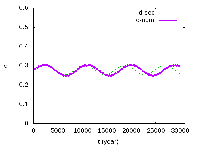
Figure 1: Evolution of eccentricity for the case of $m_{c}=2M_{J}$ and $m_{d}=4M_{J}$, using the secular perturbation, and the full numerical integration. On the left plot, we present the evolution of eccentricity for planet $c$. On the right plot, we present the evolution of eccentricity for planet $d$.

3 Numerical Simulations

Table 1: Orbital Elements for $\upsilon$ Andromedae planets from McArthur et al. (2010) and Curiel et al. (2011).

		McArthur et al. (2010)	Curiel et al. (2011)
$M_{*}$ (M⊙)		1.31	1.30
$M_{p}$ ($M_{J}$)	b	5.9	0.6876
	c	14.57	1.981
	d	10.19	4.132
	e	-	1.059
$a$ (au)	b	0.059	0.0592
	c	0.861	0.8277
	d	2.703	2.5133
	e	-	5.2455
$I$ (°)	b	6.9	-
	c	16.7	-
	d	13.5	-
	e	-	-
$e$	b	0.010	0.0215
	c	0.239	0.2596
	d	0.274	0.2987
	e	-	0.0053
$\Omega$ (°)	b	45.5	-
	c	295.5	-
	d	115.0	-
	e	-	-
$\omega$ (°)	b	41.4	324.9
	c	290.0	241.7
	d	240.8	258.8
	e	-	367.3

To verify the orbital stability of the system for different mass values for planets $c$ and $d$, we studied the temporal evolution of the eccentricity of each planet. In this study, we adopted the initial values of $a$, $e$ and $\omega$ shown in Table 1 from Curiel et al. (2011).

In the secular theory is assumed that $r_{1}<r_{2}$, where $r_{1}=r_{c}$ and $r_{2}=r_{d}$ are the distances from the central body for planets $c$ and $d$, respectively. In other words, the orbits of the two planets cannot cross. This limitation can be characterized considering the situation where the distance from the apocenter of the inner body (planet $c$) is equal to the distance from the pericenter of the outer body (planet $d$), i.e.:

$$\begin{split}a_{c}(1+e_{c})=a_{d}(1-e_{d}),\end{split}$$ (7)

where $a_{c}$, $a_{d}$ are the semi-major axes of the planets $c$ and $d$ while $e_{c}$, $e_{d}$ are the eccentricities of the planets $c$ and $d$, respectively.

Since the secular perturbation does not affect the values of the semi-major axis, we have $a_{c}$ and $a_{d}$ remaining constants. In this way, we can get the values of the critical eccentricities that indicate when the secular theory is certainly not valid and instability occurs in the system. In Figure 2, we show the relation between the eccentricities of planets $c$ and $d$, given by eq.(7). The dark gray region indicates the unstable orbits induced by the close encounter between the planets.

For the value of $e_{c}=0.2596$ (Curiel et al, 2011), we find the critical eccentricity of planet $d$ as $0.605$. For the value of $e_{d}=0.2987$ (Curiel et al, 2011), we find that the orbit of planet $c$ should be hyperbolic.This result only takes configurations where the planets’orbits cross.

In fact, even without crossing orbits, there may appear instability due to the gravitational interactions between the two planets. So, there is a minimal distance between the two orbits that can produce instability in the planetary orbits, creating a region indicated by “Transition” in Figure 2. The location and size of such region depends on the masses of the planets involved. Therefore, in Figure 2 we divided the $e_{c}\times e_{d}$ plot in three regions: one region that is unstable due to the crossing of the orbits, independent of values of the planets’ masses (dark gray region); one region that is stable (white region); and one region, located between the other two regions, that is also unstable, but its size depends on the masses of the planets. One example for the location of the green line, that mark the transition limit, will be given by equation (8).

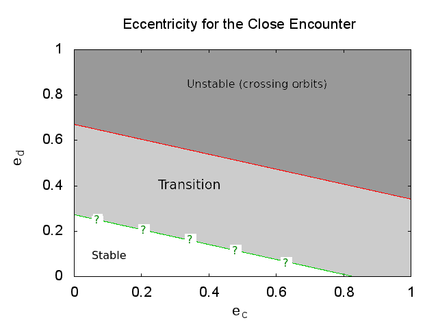
Figure 2: Relation between the critical eccentricities of the planets $c$ and $d$, according to eq. (7). The dark gray region indicates an instability area for the orbits of planets $c$ and $d$. Between the unstable and stable region (white area), it is located the transition region which takes into account the gravitational interactions between two masses even not necessarily crossing their orbits.

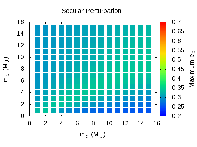
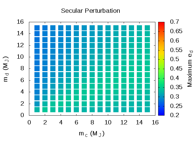
Figure 3: The maximum values of eccentricity for each value of mass using secular perturbation. On the left plot are given the maximum values for the eccentricity of planet $c$ and, on the right plot for planet $d$. Both results presented eccentricity values below $0.35$, indicating only possibly stable orbits.

To evaluate the eccentricity evolution in different cases of planets’masses in the system, we adopted a grid of masses ranging from $1M_{J}$ to $15M_{J}$ with a step of $1M_{J}$ for the masses of planets $c$ and $d$. We integrated for a total time of 30 thousand years.

We first analyze the maximum values of eccentricity for each value of mass using the secular theory. We used the initial eccentricity values of Curiel et al. (2011), given in Table 1.

Figures 3 shows the maximum values of eccentricity for planet $c$ (left plot) and for planet $d$ (right plot). The values in both cases are all smaller than $0.5$. Considering that the initial values of the eccentricities are approximately $0.26$ for planet $c$ and $0.30$ for planet $d$, we see an eccentricity increase of less than $0.2$. So, neither of them reach the critical eccentricity value. Consequently, for the whole range of masses considered, the orbits do not cross each other.

Therefore, according to the secular perturbation theory, all these orbits are stable. However, the secular theory validity is limited due to its approximations, which can be check through a comparison with full numerical integrations.

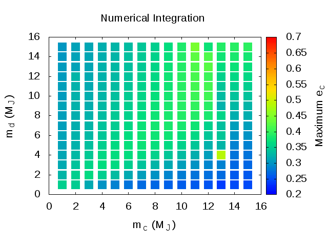
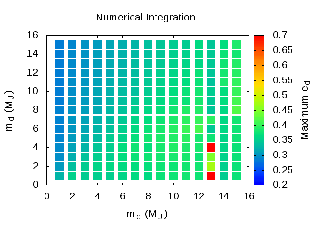
Figure 4: The maximum values of eccentricity for each value of mass using numerical integration. On the left plot are given the maximum values of eccentricity for planet $c$ and, on the right plot for planet $d$. We can see larger values of eccentricities than in the secular theory case.

We proceed similarly using the Mercury package (Chambers, 1999) to numerically integrate the system with different values of planetary masses, throught the Burlish-Stoer integrator. When numerical integrations are applied, short period terms are included which are not accommodated by secular theory.

In Figure 4, the results for planet $c$ (left plot) do not present any case with an eccentricity larger than $0.5$. However, planet $d$ (right plot) has two possibilities of planets ejection, which occur at the red squares, meaning that the eccentricity is larger than the critical value and the orbits of the planets cross each other. The cases in the region of masses close to the ejection results (red squares) also present instability, but for the integration time used here (30 thousands years) there is no ejection, which does not exclude the possibility when integrated longer timescales. We performed a careful a visual inspection of the evolution of the eccentricity plots for all cases simulated in the grid of masses and we verified that from $m_{c}$ greater than $8M_{J}$ the temporal evolution of the planets eccentricities show instability.

Comparing Figures 3 and 4, we see that the secular theory results reproduce the general trend of values of the maximum eccentricities according to the planetary masses. However, these values are smaller than the actual values, generated from the numerical integrations.

In the present study, we aim to gauge the extent to which secular theory can be used with the same accuracy as numerical integration. To analyze the discrepancies between the two methods, we compare the difference between the amplitudes of eccentricity variation for each case of planetary mass, that is, the difference between the highest value and the lowest value of the eccentricity of the planets.

The plots in Figure 5 present the amplitudes of oscillation of the eccentricities of the planets for the case of the secular theory. These amplitudes are all smaller than $0.35$.

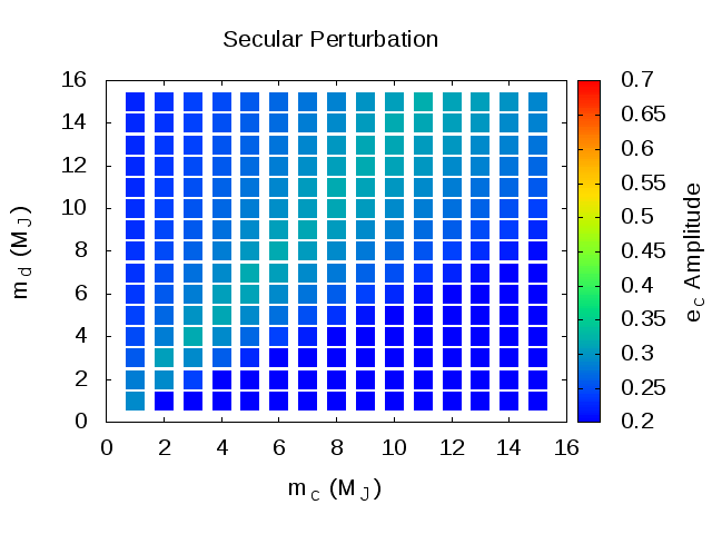
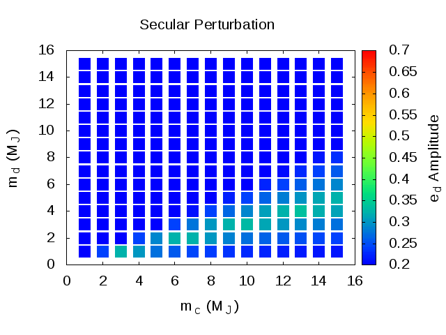
Figure 5: Amplitude of the eccentricity variation for planets $c$ and $d$ according to the different values of masses (in Jupiter masses) using secular theory. On the color palette we have eccentricity amplitude values. On the left plot, we observe the amplitude of the eccentricity of planet $c$. The right plot shows the results for planet $d$.

For the case of the numerical integrations, the amplitudes of oscillation of the eccentricities are shown in Figure 6. For planet $c$ the amplitude can get up to $0.5$, while for planet $d$ there is a couple of orbits that reach values even higher.

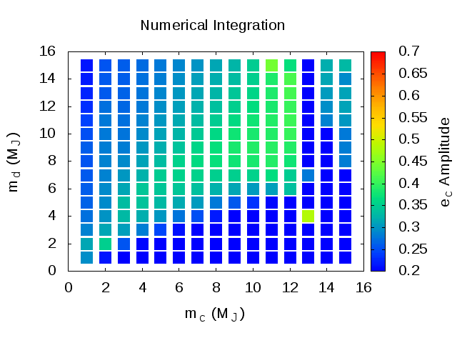
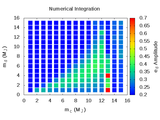
Figure 6: Amplitude of the eccentricity variation for planets $c$ and $d$ according to the different values of masses (in Jupiter masses) for the numeral integration. On the color palette we have eccentricity amplitude. On left we observed the amplitude of the eccentricity of the planet $c$. On the right the figure shows the results for the planet $d$.

4 Validity for The Secular Theory

In order to evaluate how good were the secular theory results in comparison with the full numerical integration, we computed $\Delta e_{num}-\Delta e_{sec}$, where $\Delta e_{num}$ corresponds to the amplitude of oscillations of eccentricities from the numerical integration and $\Delta e_{sec}$ is the amplitude of oscillation of the eccentricities from the secular theory.

A first analysis of the results showed in Figure 7 indicates that the secular theory works better for the inner planet (left plot) than for the outer planet (right plot). It is also better for lower values of the masses. In the case of planet $c$ (inner planet) the best results occurred for $m_{c}$ $\leq$ $7$$M_{J}$ and for $7$$M_{J}$ $<$ $m_{c}$ $<$ $12$$M_{J}$ with $m_{d}$ $\leq$ $5$$M_{J}$. In the case of planet $d$ (outer planet) the best results occurred only for $m_{c}$ $<$ $4$$M_{J}$ with $m_{d}$ $>$ $2$$M_{J}$.

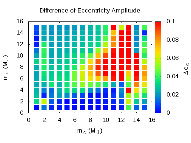
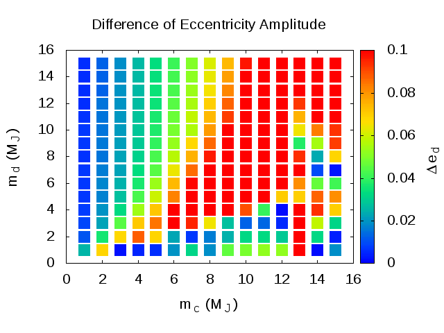
Figure 7: Difference of the eccentricities amplitude between the numerical integration results and the secular theory results for planets $c$( left) and $d$ (right) according to the variation of the masses (in Jupiter masses).

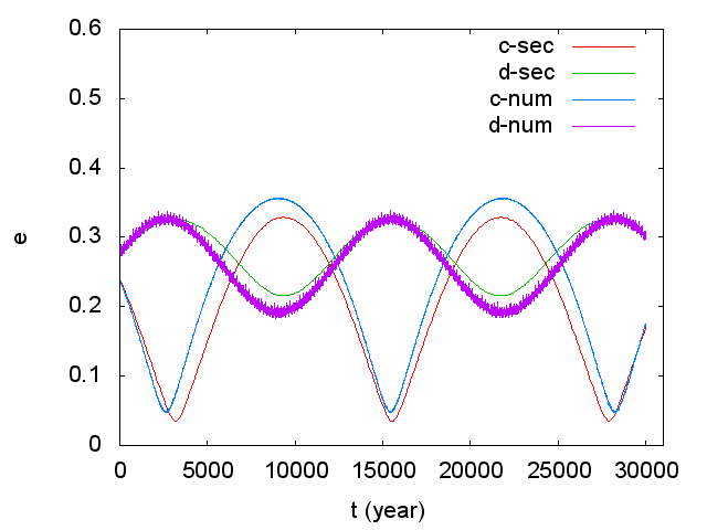
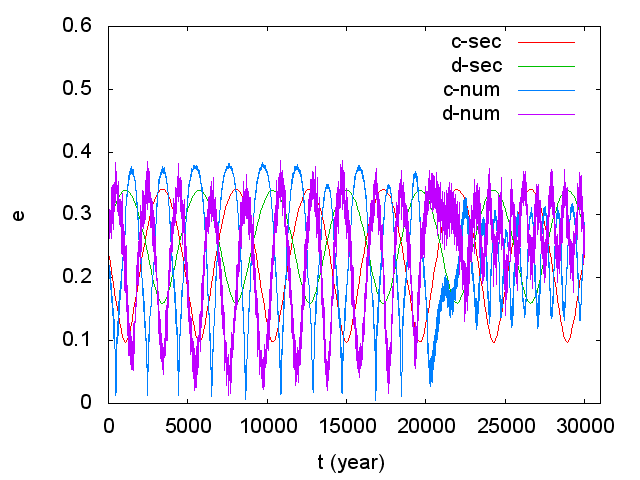
Figure 8: Evolution of eccentricity for planets $c$ and $d$. The evolution of eccentricity by the secular theory is in red for planet $c$ and in green by the planet $d$. The eccentricity evolution by the numerical integration is in blue for planet $c$ and in purple for planet $d$. On the left plot, we have the stable case for $m_{c}=3M_{J}$ and $m_{d}$ $=$ $3$ $M_{J}$. In the right plot, we exemplify a chaotic case of eccentricity evolution, in this case $m_{c}$ $=$ $12$ $M_{J}$ and $m_{d}$ $=$ $8$ $M_{J}$.

In Figure 8, we present two cases to exemplify the possible destinations for the planetary dynamical evolution. In the first case, on the left plot, with planetary masses equal to $3$ $M_{J}$ for planets $c$ and $d$, we have a stable case. This case could be used to draw the green line on figure 2, as we show in eqation (8) for the case $m_{c}=13M_{J}$ and $m_{d}=1M_{J}$. But, for this case, the green line will be located in a different position because the planetary masses are different and as a consequence the gravitational interactions change.

The planets eccentricity variation are very similar in numerical integration and in secular theory. Note that in the numerical integration, planet $d$ has a secondary frequency. This secondary frequency is due to the short period terms, which are considered in numerical integration, but they are not included in the secular theory. The second case, on the right plot, for the masses $m_{c}=12M_{J}$ and $m_{d}=8M_{J}$ shows an unstable behavior for the numerical integration, but in the secular theory, as expected, we always have stable orbits.

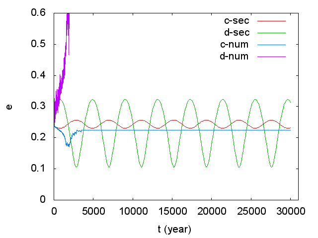
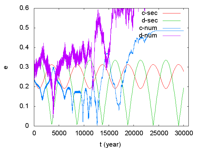
Figure 9: Evolution of the eccentricity for planets c and d in the ejected cases. The evolution of eccentricity in the secular theory is in red for planet $c$ and in green for planet $d$. The eccentricity evolution from the numerical integration is in blue for planet $c$ and in purple for planet $d$. On the left plot, we have the case for the masses of $c$ equal to $13$ $M_{J}$ and $d$ equal to $1$ $M_{J}$. In the right plot, we have the eccentricity evolution, for the masses of $c$ equal to $13$ $M_{J}$ and $d$ equal to $4$ $M_{J}$.

From Figure 4, we have that when $m_{c}=13M_{J}$ and $m_{d}=4M_{J}$, both planets showed large variations in their eccentricities. The orbit of the two planets were so unstable that planet $d$ was ejected. The same occurred for the case when $m_{c}=13M_{J}$ and $m_{d}=1M_{J}$. The evolution of the eccentricity, in these two cases of ejection, are shown in Figure 9. We consider that, in order to ejection occurs in the numerical integration, the semi-major axis has to be greater than $100$ $au$.

The left plot shows that planet $d$ is ejected in less than two thousand years, while in the other case it is ejected much later, in $25$ thousand years. In both cases the systems show a highly unstable behavior since the beginning of the integration.

Therefore, the examples shown here cover the whole spectrum. A case of planetary masses where the secular theory reproduces very well the orbital evolution of the system (Figure 8, left). A case where the planetary masses are such that the evolution of the eccentricities of the planets have their limits reproduced by the secular theory, but not following the same pattern of of behavior (Figure 8, right). And finally, two cases where the planetary masses are so big that the secular theory is of no use at all (Figure 9).

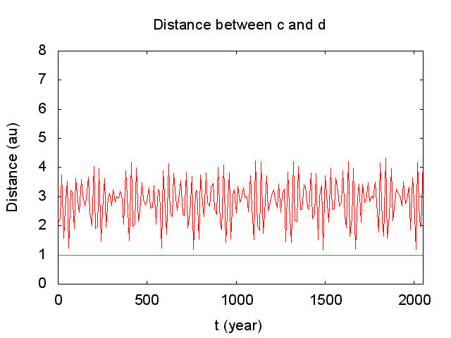
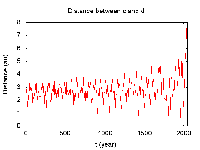
Figure 10: Distance between planets $c$ and $d$ for two thousand years. On the left plot, we present the stable case, with masses of the two planets of $3$ $M_{J}$. On the right plot, the unstable case with ejection, for the masses of $c$ equal to $13$ $M_{J}$ and $d$ equal to $1$ $M_{J}$. The green line indicated the distance of $1$ $au$.

Next, we calculated the distance between the planets $c$ and $d$, to try detect if there are close encounters between the two planets, which could be the cause of the ejection of planet $d$. In Figure 10, we show the distance between the planets in a stable case, on the left plot, with masses of the two planets equal to $3$ $M_{J}$. We can observe that the planets are never less than one astronomical unit from each other (green line). Whereas, on the right, we presented the ejection case, for the planets with mass $c$ equal to $13$ $M_{J}$ and $d$ equal to $1$ $M_{J}$, there is a close encounter in less than one thousand years, the approach between the planets decay to less than one astronomical unit.

Based on our discussion of close planetary encounters made in Figure 2, we have a limiting distance between the planets of 1 AU, for the masses $m_{c}=13M_{J}$ and $m_{d}=1M_{J}$, so, equation (7) can be rewritten as

$$\begin{split}|a_{c}(1+e_{c})-a_{d}(1-e_{d})|=1,\end{split}$$ (8)

where $a_{c}$ and $a_{d}$ are the semi-major axis of the planets $c$ and $d$, respectively, and $e_{c}$ and $e_{d}$ are the eccentricities of the planets $c$ and $d$.

Now, we can define a lower limit of eccentricities for planets with such masses, beyond which the orbits would be unstable. This limit corresponds to the lower curve defining the Transition region shown in Figure 2.

All analyses reported in this study were conducted using a planar case of a planetary system. In cases with inclination it is possible that planets with large masses have stable orbits and it can be explored in future works.

5 Conclusions

The literature on the planetary system of $\upsilon$ Andromedae presents a wide discrepancy for the planetary masses. In the present work, we study the stability of planets $c$ and $d$ as a function of their masses in order to contribute for the delimitation of their possible masses. We studied the temporal evolution of the eccentricity of each planet using two approaches. First adopting the Lagrange-Laplace secular theory and then through the full numerical integration. We used the two methods to compare and check the limits of the validity of the secular theory.

The results obtained in this work show that the use of secular theory can infer the stability of a planetary system but only for a limited range of values for the planetary masses. For high values of mass, the numerical integration becomes the best choice, mainly due the fact that the secular theory does not take into account short period terms.

With the numerical integration, we found the limits for the planetary masses to allow the orbital stability of the planets. For planetary masses larger than $8M_{J}$ for planet $c$, independently of the mass for planet d, an unstable behavior is almost certain and possibilities of ejection of the planets exist.

As expected, we verified that above critical eccentricity values the orbits cross each other, which leads to instability and possible ejection. We also identified an unstable region without the need of crossing orbits, whose size depends on the values of the planets’masses.

References

- [1] Barnes R, Grennberg R, Quinn TR, McArthur BE, Benedict GF (2011) Origin and dynamics of the mutually inclined orbits of Andromedae c and d. The Astrophysical Journal 726:71
- [2] Butler RP, Marcy GW, Hauser EW, Shirts P (1997) Three new “51 Pegasi-type” planets. The Astrophysical Journal 474:L115-L118
- [3] Chambers JE (1999) A hybrid sympletic integrator that permits close encounters between massive bodies. Monthly Notices of the Royal Astronomical Society 304:793-799
- [4] Curiel S, Cantó J, Georfie, L, Chavez CE, Poveda A (2011) A fourth planet orbiting Andromedae. Astronomy and Astrophysics 525:1-5
- [5] Gomes RS, Matese JJ, Lissauer JJ (2006) A distant planetary-mass solar companion may have produced distant detached objects. Icarus 184:589-601
- [6] Han E, Wang SX, Wright JT, Feng YK, Zhao M, Fakhouri O, Brown JI, Hancock C (2014) Exoplanet orbit database. II. Updates to exoplanets.org the Astronomical Society of Pacific 126:827-837
- [7] McArthur BE, Benedict GF, Barnes R, Martioli E, Korzennik S, Nelan E, Butler RP (2010) New observational constraints on the Andromedae system with data from the Hubble Space Telescope and Hobby-Eberly Telescope. The Astrophysical Journal 715:1203-1220
- [8] Murray CD, Dermott SF (1999) Solar System Dynamics. Cambrige University Press, Cambridge