Approximation of Hermitian Matrices by
Positive Semidefinite Matrices using
Modified Cholesky Decompositions

Abstract

A new algorithm to approximate Hermitian matrices by positive semidefinite Hermitian matrices based on modified Cholesky decompositions is presented. In contrast to existing algorithms, this algorithm allows to specify bounds on the diagonal values of the approximation.

It has no significant runtime and memory overhead compared to the computation of a classical Cholesky decomposition. Hence it is suitable for large matrices as well as sparse matrices since it preserves the sparsity pattern of the original matrix.

The algorithm tries to minimize the approximation error in the Frobenius norm as well as the condition number of the approximation. Since these two objectives often contradict each other, it is possible to weight these two objectives by parameters of the algorithm. In numerical experiments, the algorithm outperforms existing algorithms regarding these two objectives.

A Cholesky decomposition of the approximation is calculated as a byproduct. This is useful, for example, if a corresponding linear equation should be solved.

A fully documented and extensively tested implementation is available. Numerical optimization and statistics are two fields of application in which the algorithm can be of particular interest.
 

1 Introduction

Algorithms for approximating Hermitian matrices by positive semidefinite Hermitian matrices are useful in several areas. In stochastics they are needed to transform nonpositive semidefinite estimations of covariance and correlation matrices to valid estimations Rousseeuw1993 ; Qi2010 ; Higham2002a ; Higham2016b . In optimization they are needed to deal with nonpositive definite Hessian matrices in Newton type methods Gill1981 ; Nocedal2006 ; Chong2013 .

The existing algorithms have different disadvantages, which will be outlined below. A new algorithm without these disadvantages is presented in Section 2 where it is also examined in detail. An implementation is introduced in Section 3 together with numerical experiments and corresponding results. Conclusions are drawn in Section 4.

1.1 Objectives of approximation algorithms

In order to evaluate the existing algorithms, objectives of an ideal approximation algorithm are established. For this, let $A\in\mathbb{C}^{n\times n}$ be an Hermitian matrix and $B\in\mathbb{C}^{n\times n}$ its approximation. The first three objectives are the following:

1. $B$ is positive semidefinite.

1. The approximation error $\|B-A\|$ is small.

1. The condition number $\kappa(B)=\|B\|\,\|B^{-1}\|$ is small.

In addition to the approximation error, the condition number of the approximation is usually important as well, since, for example, often linear equations including the approximation have to be solved.

The three objectives (O1), (O2) and (O3) are sometimes contradictory. Hence, an ideal algorithm would allow to prioritize between (O2) and (O3). The norm used in (O2) and (O3) may depend on the actual application. Typical choices are the spectral norm or the Frobenius norm.

Especially for large matrices, the execution time of the algorithm as well as the needed memory are important. The fastest way to test whether a matrix is positive definite is to try to calculate its Cholesky decomposition Higham1988 . This needs $\tfrac{1}{3}n^{3}+\mathcal{O}(n^{2})$ basic operations in the dense real valued case. The approximation algorithm cannot be expected to be faster but at least asymptotically as fast. Thus, the next two objectives are:

1. The algorithm requires at most $\mathcal{O}(n^{2})$ more basic operations than the calculation of a Cholesky decomposition of $B$.

1. The algorithm needs to store $\mathcal{O}(n)$ numbers besides $A$ and $B$ and allows to overwrite $A$ with $B$.

If $A$ is a sparse matrix, $B$ should have the same sparsity pattern. This allows an effective overwriting and is essential if the corresponding dense matrix would be to big to store. Thus, the next objective is:

1. $A_{ij}=0$ implies $B_{ij}=0$.

For correlation matrices it is crucial that $B$ has only ones as diagonal values. This is the reason for the last objective:

1. The diagonal of $B$ can be predefined.

Similar objectives to (O1), (O2), (O3) and (O4) have been used in Schnabel1990 ; Schnabel1999 ; Cheng1998 ; Fang2008 . Here, another objective has been established: If $A$ is ”sufficiently” positive definite, $B$ should be equal to $A$. This objective is not explicitly listed here and should be covered by (O2).

1.2 Existing approximation methods

An overview of existing methods to approximate Hermitian matrices by positive semidefinite Hermitian matrices is provided next. They are evaluated using the objectives mentioned above.

The minimal approximation error can be achieved by computing an eigendecomposition and replacing negative eigenvalues Higham1988 ; Higham1989 . This was done in statistics Iman1982 ; Rousseeuw1993 as well as in optimization (Nocedal2006, , Chapter 3.4), (Gill1981, , Chapter 4.4.2.1). However, this does not meet (O4), (O6) and (O7).

It is also possible to calculate approximations with minimal approximation error and the restriction that all diagonal values are one Higham2002a ; Borsdorf2010 ; Borsdorf2010a ; Higham2016 . These methods could be extended so that the approximation has arbitrary predefined (nonnegative) diagonal values. Nevertheless, these methods do not meet (O4) and (O6).

Another method, especially common in optimization, is to add a predefined positive definite matrix multiplied by a sufficiently large scalar to the original matrix. The predefined matrix is usually the identity matrix or a diagonal matrix. The scalar is usually determined by increasing a value until the resulting approximation can be successfully Cholesky factorized. This method is also used in a modified Newton’s method Goldfeld1966 ; Chong2013 ; Nocedal2006 and the Levenberg-Marquardt method Levenberg1944 ; Marquardt1963 ; Chong2013 . However, (O4) and (O7) are not met.

A well-known method, in statistics, is a convex combination with a predefined positive definite matrix. In this context it is based on the concept of shrinkage estimator Stein1956 ; Devlin1975 ; Rousseeuw1993 . The positive definite matrix is again usually the identity matrix or a diagonal matrix. Only the convex combination factor has to be determined. This is usually done by examining the underlying statistical problem Chen2010 ; Fisher2011 ; Ikeda2016 ; Ledoit2003 ; Ledoit2004 ; Schaefer2005 ; Touloumis2015 . However, methods without using any statistical assumptions exist as well Higham2016b . None of these meet (O4) and (O7).

Other methods used, especially in optimization, are modified Cholesky algorithms Gill1974 ; Gill1981 ; Schnabel1990 ; Schnabel1999 ; More1979 ; Cheng1998 ; Fang2008 . These compute a variant of a Cholesky decomposition like a $LDL^{T}$, a $LBL^{T}$ or a $LTL^{T}$ decomposition. Here $L$ is a lower triangular matrix, $D$ is a diagonal matrix, $B$ is a block diagonal matrix with block size smaller of one or two and $T$ is a tridiagonal matrix. During or after the calculation of these decompositions, their factors are modified so that they represent a positive definite matrix. The methods based on $LBL^{T}$ decomposition More1979 ; Cheng1998 do not meet (O4), (O6) and (O7), the ones based on $LTL^{T}$ decomposition Fang2008 do not meet (O6) and (O7) and the ones based on $LDL^{T}$ decomposition Gill1974 ; Gill1981 ; Schnabel1990 ; Schnabel1999 ; Fang2008 do not meet (O7).

Hence, none of the existing methods meet all objectives. However, methods that do not meet (O7) can be extended to meet this objective. For that the calculated approximation is multiplied by a suitable chosen diagonal matrix from both sides. This does not affect (O1), (O4), (O5) and (O6). So the modified Cholesky method based on $LDL^{T}$ decomposition could meet all objectives if they are extended to meet (O7).

The new method presented in Section 2 is a modified Cholesky method based on $LDL^{T}$ decomposition as well. Contrary to the already published methods of this kind, this methods modifies not only the matrix $D$ but also the matrix $L$ during their calculation. In this way, the algorithm meets all objectives. Furthermore it better meets (O2) and (O3) than the other extended methods based on $LDL^{T}$ decomposition as shown in Section 3 by numerical experiments.

2 The approximation algorithm

The algorithm MATRIX which approximates Hermitian matrices by positive semidefinite matrices Hermitian is presented and analyzed in this section.

2.1 The MATRIX and the DECOMPOSITION algorithm

Previous modified Cholesky methods based on $LDL^{T}$ decomposition Gill1974 ; Gill1981 ; Schnabel1990 ; Schnabel1999 ; Fang2008 applied to a symmetric matrix $A$ try to calculate its $LDL^{T}$ decomposition. While doing so, they increase some of the values in the diagonal matrix $D$. Hence, they result in a decomposition of a positive definite matrix $A+\Delta$, where $\Delta$ is a diagonal matrix with values greater or equal to zero. However, is this way, the approximation $A+\Delta$ cannot have predefined diagonal elements.

The key idea of the new algorithm is to modify the off-diagonal values of $A$ instead or in addition to its diagonal values. In detail, the Hermitian positive definite approximation $B\in\mathbb{C}^{n\times n}$ of an Hermitian $A\in\mathbb{C}^{n\times n}$ is defined as

$$B_{ij}:=\hat{\omega}_{ij}A_{ij}\text{ if }i\neq j\text{ and }B_{ii}:=A_{ii}+\delta_{i}$$

where $\hat{\omega}_{ij}\in[0,1]$, $\hat{\omega}_{ij}=\hat{\omega}_{ji}$ and $\delta_{i}\in\mathbb{R}$ for all $i,j\in\{1,\ldots,n\}$.

If, for example, $\hat{\omega}_{ij}=0$ and $\delta_{i}>|A_{ii}|$ for all $i,j\in\{1,\ldots,n\}$, then $B$ is a diagonal matrix with only positive values and thus positive definite. If, on the other hand, $\hat{\omega}_{ij}=1$ and $\delta_{i}=0$ for all $i,j\in\{1,\ldots,n\}$, then $B=A$ and there is no approximation error.

The challenge is now to determine the values $\hat{\omega}_{ij}$ and $\delta_{i}$ such that the objectives established in Subsection 1.1 are met. This is where we use a (complex valued) modified Cholesky method based on $LDL^{H}$ decomposition. During the calculation of a $LDL^{H}$ decomposition of $A$, we modify $L$ and $D$ if the matrix represented by the decomposition would become not positive definite, its condition number would become to high or the requirements on the diagonal values would be violated otherwise.

In detail, the off-diagonal values in the $i$-th row of $L$ are multiplied by $\omega_{i}\in[0,1]$ and $\delta_{i}\in\mathbb{R}$ is added to the $i$-th diagonal value of $D$. This $\delta_{i}$ corresponds to the previously mentioned $\delta_{i}$ and $\omega$ to $\hat{\omega}$ such that $\hat{\omega}_{i,j}=\omega_{\max\{{i,j}\}}$ for all $i,j\in\{1,\ldots,n\}$. This relationship is discussed in Subsection 2.2. Furthermore symmetric permutation techniques are used to reduce the approximation error, the computational effort and the required memory.

The algorithm DECOMPOSITION, which computes the permuted modified $LDL^{H}$ decomposition and the values $\omega$ and $\delta$, is described in detail in Algorithm 1.

Algorithm 1 DECOMPOSITION

1:Input: $\cdot$ $A\in\mathbb{C}^{n\times n}$ Hermitian, $x\in(\mathbb{R}\cup\{-\infty\})^{n}$, $y\in(\mathbb{R}\cup\{\infty\})^{n}$, $l\in\mathbb{R}\cup\{-\infty\}$, $u\in\mathbb{R}\cup\{\infty\}$, $\epsilon>0$ $\cdot$ with $\max\{x_{i},l\}\leq\min\{y_{i},u\}$ for all $i\in\{1,\ldots,n\}$ $\cdot$ with $|x_{i}|,|l|\geq\epsilon$ or $|y_{i}|,|u|\geq\epsilon$ for all $i\in\{1,\ldots,n\}$

2:Output: $\cdot$ $L\in\mathbb{C}^{n\times n}$, $d,\omega,\delta\in\mathbb{R}^{n}$, $p\in\{1,\ldots,n\}^{n}$

3:function decomposition($A,x,y,l,u,\epsilon$)

4:     $p_{i}\leftarrow i$ for all $i\in\{1,\ldots,n\}$

5:     $\alpha_{i}\leftarrow 0$ for all $i\in\{1,\ldots,n\}$

6:     for $i\leftarrow 1,\ldots,n$ do

7:         select $j\in\{i,\ldots,n\}$

8:         swap $p_{i}$ with $p_{j}$ and $L_{ik}$ with $L_{jk}$ for all $k\in\{1,\ldots,i-1\}$

9:         select $d_{i}\in[l,u]$, $\omega_{p_{i}}\in[0,1]$ with $|d_{i}|\notin(0,\epsilon)$, $d_{i}+\alpha_{p_{i}}\omega_{p_{i}}^{2}\in[x_{p_{i}},y_{p_{i}}]$

10:         $L_{ij}\leftarrow\omega_{p_{i}}L_{ij}$ for all $j\in\{1,\ldots,i-1\}$

11:         $\delta_{p_{i}}\leftarrow d_{i}+\omega_{p_{i}}^{2}\alpha_{p_{i}}-A_{p_{i}p_{i}}$

12:         for $j\leftarrow i+1,\ldots,n$ do

13:              if $d_{i}\neq 0$ then

14:                  $L_{ji}\leftarrow\left(A_{p_{j}p_{i}}-\sum\limits_{k=1}^{i-1}L_{jk}\overline{L}_{ik}d_{k}\right)(d_{i})^{-1}$

15:                  $\alpha_{p_{j}}\leftarrow\alpha_{p_{j}}+|L_{ji}|^{2}d_{i}$

16:              else

17:                  $L_{ji}\leftarrow 0$

18:              end if

19:         end for

20:     end for

21:     $L_{ii}\leftarrow 1$ and $L_{ij}\leftarrow 0$ for all $i,j\in\{1,\ldots,n\}$ with $j>i$

22:     return $(L,d,p,\omega,\delta)$

23:end function

The algorithm MATRIX, which computes the approximation $B$, is described in detail in Algorithm 2.

Algorithm 2 MATRIX

1:Input: $\cdot$ $A\in\mathbb{C}^{n\times n}$ Hermitian, $x\in(\mathbb{R}\cup\{-\infty\})^{n}$, $y\in(\mathbb{R}\cup\{\infty\})^{n}$, $l\in\mathbb{R}\cup\{-\infty\}$, $u\in\mathbb{R}\cup\{\infty\}$, $\epsilon>0$ $\cdot$ with $\max\{x_{i},l\}\leq\min\{y_{i},u\}$ for all $i\in\{1,\ldots,n\}$ $\cdot$ with $|x_{i}|,|l|\geq\epsilon$ or $|y_{i}|,|u|\geq\epsilon$ for all $i\in\{1,\ldots,n\}$

2:Output: $\cdot$ $B\in\mathbb{C}^{n\times n}$

3:function matrix($A,x,y,l,u,\epsilon$)

4:     $(L,d,p,\omega,\delta)\leftarrow$ DECOMPOSITION($A,x,y,l,u,\epsilon$)

5:     $q_{p_{i}}\leftarrow i$ for all $i\in\{1,\ldots,n\}$

6:     for $i\leftarrow 1,\ldots,n$ do

7:         $B_{ii}\leftarrow A_{ii}+\delta_{i}$

8:         for $j\leftarrow i+1,\ldots,n$ do

9:              if $q_{i}>q_{j}$ then

10:                  $a\leftarrow j$, $b\leftarrow i$

11:              else

12:                  $a\leftarrow i$, $b\leftarrow j$

13:              end if

14:              if $d_{q_{a}}\neq 0$ or $\omega_{b}=0$ then

15:                  $B_{ij}\leftarrow A_{ij}\omega_{b}$

16:              else

17:                  $B_{ij}\leftarrow\sum\limits_{k=1}^{q_{a}-1}L_{q_{i}k}d_{k}\overline{L}_{q_{j}k}$

18:              end if

19:         end for

20:     end for

21:     $B_{ji}\leftarrow\overline{B}_{ij}$ for all $i,j\in\{1,\ldots,n\}$ with $j>i$

22:     return $B$

23:end function

The parameters $l$ and $u$ of the algorithms are lower and upper bounds on the diagonal values of $D$. The positive definiteness of $B$ can be controlled by $l$ as pointed out in Subsection 2.3. The parameters $x$ and $y$ are lower and upper bounds on the diagonal values of $B$ as shown in Subsection 2.4. The condition number of $B$ and the approximation error $\|B-A\|$ are influenced by $x,y,l,u$ as demonstrated in Subsection 2.5 and 2.6, respectively. Moreover, they allow to prioritize a low approximation error or a low condition number. The numerical stability of the algorithms is controlled by $\epsilon$.

The algorithms can be considered as a whole class of algorithms since there are many possibilities to choose the permutation and $\omega$ and $\delta$ as discussed in Subsection 2.7 and 2.8. The algorithm is carefully designed, so that the overhead in computational effort and memory consumption compared to classical Cholesky decomposition algorithms is negligibly if $\omega$ and $\delta$ are chosen in a proper way, as shown in Subsection 2.9.

For the rest of this section, we use the following notation for the analysis of both algorithms.

Definition 1

Let

$$B:=\text{\nameref{alg: approximated matrix}}(A,x,y,l,u,\epsilon)$$

where $(A,x,y,l,u,\epsilon)$ is some valid input for the algorithm with $A\in\mathbb{C}^{n\times n}$ and

$$(L,d,p,\omega,\delta):=\text{\nameref{alg: approximated decomposition}}(A,x,y,l,u,\epsilon).$$

Define $D:=\operatorname{diag}(d)$ the diagonal matrix with $d$ as the diagonal. Define $P\in\mathbb{R}^{n\times n}$ as the permutation matrix induced by $p$, which is

$$P_{ij}:=\begin{cases}1\text{ if }j=p_{i}\\ 0\text{ else}\end{cases}\text{ for all }i,j\in\{1,\ldots,n\}.$$

2.2 Representation of the approximation matrix

In this subsection it is shown that $B=P^{T}LDL^{H}P$. This means that MATRIX calculates the matrix represented by the decomposition calculated by DECOMPOSITION. This will be crucial for further investigation of MATRIX.

First, we prove that $p$ is a permutation vector.

Lemma 1

$$\{p_{i}~{}|~{}i\in\{1,\ldots,n\}\}=\{1,\ldots,n\}.$$

Proof

In DECOMPOSITION, the variable $p$ is initiated at line 4 of the algorithm so that $p_{i}=i$ for all $i\in\{1,\ldots,n\}$. After its initialization, the variable $p$ is only changed in line 8. Here some of its components are swapped in each iteration. Thus $\{p_{i}~{}|~{}i\in\{1,\ldots,n\}\}=\{1,\ldots,n\}$ at the end of the algorithm.

Next it is shown how a corresponding inverse permutation vector can be defined.

Lemma 2

Define

$$q_{p_{i}}:=i\text{ for all }i\in\{1,\ldots,n\}.$$

$q$ is well defined and

$$p_{q_{i}}=i\text{ for all }i\in\{1,\ldots,n\}.$$

Proof

$q$ is well defined due to Lemma 1. Let $i\in\{1,\ldots,n\}$. Due to Lemma 1, a $j\in\{1,\ldots,n\}$ exists with $p_{j}=i$. Furthermore $q_{p_{j}}=j$ due to the definition of $q$. Thus, $p_{q_{i}}=p_{q_{p_{j}}}=p_{j}=i$ follows.

A fast way to calculate $LDL^{H}$, using only $A$, $\omega$, $\delta$ and $p$, is pointed out in the next lemma.

Lemma 3

$$(LDL^{H})_{ii}=A_{p_{i}p_{i}}+\delta_{p_{i}}$$

and

$$(LDL^{H})_{ij}=A_{p_{i}p_{j}}\omega_{p_{\max\{i,j\}}}\text{ if }d_{\min\{i,j\}}\neq 0\text{ or }\omega_{p_{\max\{i,j\}}}=0$$

for all $i,j\in\{1,\ldots,n\}$ with $i\neq j$.

Proof

First some properties of the variable $p$ during the execution of the algorithm are proved. Denote the for loop starting at line 6 of the algorithm the main for loop. Let $p^{(0)}$ be the value of the variable $p$ directly before the main for loop and $p^{(i)}$ its value directly after its $i$-th iteration for each $i\in\{1,\ldots,n\}$. Its final value is denoted by $p$.

Let $i\in\{1,\ldots,n\}$. The variable $p$ is initiated so that $p^{(0)}_{i}=i$. After its initialization, the variable $p$ is only changed in line 8. Here the variables $p_{i}$ and $p_{j}$ are swapped for some $j\in\{i,\ldots,n\}$ in the $i$-th iteration of the main for loop. Hence

$$\{p_{i}^{(j)}~{}|~{}i\in\{1,\ldots,n\}\}=\{1,\ldots,n\}\ \text{ for all }j\in\{1,\ldots,n\}.$$ (1)

Furthermore the variable $p_{i}$ is not changed anymore after the $i$-th iteration. Thus

$$p_{i}=p_{i}^{(j)}\text{ for all }i,j\in\{1,\ldots,n\}\text{ with }i\leq j$$ (2)

and hence

$$p_{i}^{(i)}\neq p_{j}^{(j)}\text{ for all }i,j\in\{1,\ldots,n\}\text{ with }i\neq j.$$ (3)

Next it is shown that all entries in the variables $d$, $\omega$ and $\delta$ are set once in the algorithm and are never changed after that. Hence, we do not need an index indicating the current iteration for this variables. Let $d$, $\omega$ and $\delta$ be the final value of the corresponding variables.

The value of $d_{i}$ is set in the $i$-th iteration of the main for loop at line 9 and nowhere else. The values of $\omega_{p_{i}}$ and $\delta_{p_{i}}$ are set in the $i$-th iteration of the main for loop at line 9 and line 11 and due to (3) nowhere else. Furthermore $\omega_{i}$ and $\delta_{i}$ are set due to equation (2) and Lemma 1. Hence, all entries in the variables $d$, $\omega$ and $\delta$ are set once in the algorithm and are never changed after that.

Next properties of the variable $L$ in the algorithm are proved which will lead to the result of this lemma. Denote with $L^{(i)}$ the value of the variable $L$ directly after the $i$-th iteration of the main for loop for all $i\in\{1,\ldots,n\}$. $L$ denotes its final value.

Let $i,j\in\{1,\ldots,n\}$ with $j<i$. The variable $L_{ij}$ is only changed in the $j$-th iteration at line 14 or line 17, in the $i$-th iteration at line 10 and maybe in the $k$-th iteration at line 8 for $k\in\{j+1,\ldots,i\}$. Thus, after the $i$-th iteration it is unchanged which means

$$\begin{gathered}L_{ij}=L_{ij}^{(k)}\text{ for all }i,j,k\in\{1,\ldots,n\}\text{ with }j<i\leq k.\end{gathered}$$ (4)

In the $i$-th iteration, the variable $L_{ij}$ might only be changed in line 8 and line 10. In line 8 the variable $L_{ij}$ is only changed if it is swapped with the variable $L_{kj}$ for some $k\in\{i+1,\ldots,n\}$. This is exactly the case if the variable $p_{i}$ is swapped with the variable $p_{k}$. This together with line 10 and equation (1) implies

$$\begin{gathered}L_{ij}^{(i)}=\omega_{p_{i}^{(i)}}L_{kj}^{(i-1)}\text{ if }p_{i}^{(i)}=p_{k}^{(i-1)}\\ \text{ for all }i,j,k\in\{1,\ldots,n\}\text{ with }j<i.\end{gathered}$$

This results with equation (2) and (4) in

$$\begin{gathered}L_{ij}=\omega_{p_{i}}L_{kj}^{(i-1)}\text{ if }p_{i}=p_{k}^{(i-1)}\\ \text{ for all }i,j,k\in\{1,\ldots,n\}\text{ with }j<i.\end{gathered}$$ (5)

In the $k$-th iteration for all $k\in\{j+1,\ldots,i-1\}$, the variable $L_{ij}$ might only be changed in line 8 due to a swap with the variable $L_{kj}$. This is exactly the case if the variable $p_{i}$ is swapped with the variable $p_{k}$. This together with equation (1) implies

$$\begin{gathered}L_{ij}^{(l)}=L_{kj}^{(l-1)}\text{ if }p_{i}^{(l)}=p_{k}^{(l-1)}\\ \text{ for all }i,j,k,l\in\{1,\ldots,n\}\text{ with }j<l<i.\end{gathered}$$ (6)

Equation (5) and (6) result in

$$\begin{gathered}L_{ij}=\omega_{p_{i}}L_{kj}^{(l)}\text{ if }p_{i}=p_{k}^{(l)}\\ \text{ for all }i,j,k,l\in\{1,\ldots,n\}\text{ with }j\leq l<i.\end{gathered}$$ (7)

Now with this preparatory work, the main statement of this lemma can be proved. $L_{jj}=1$ and $L_{jk}=0$ for all $k\in\{j+1,\ldots,n\}$ due to line 21. This implies

$$(LDL^{H})_{ij}=\sum\limits_{k=1}^{n}L_{ik}\overline{L}_{jk}d_{k}=L_{ij}d_{j}+\sum\limits_{k=1}^{j-1}L_{ik}\overline{L}_{jk}d_{k}.$$

Due to equation (1), a $l\in\{1,\ldots,n\}$ exists with $p_{i}=p_{l}^{(j)}$. Hence, equation (4) and (7) imply

$$L_{ij}d_{j}+\sum\limits_{k=1}^{j-1}L_{ik}\overline{L}_{jk}d_{k}=L_{ij}d_{j}+\sum\limits_{k=1}^{j-1}L_{ik}\overline{L}_{jk}^{(j)}d_{k}=\omega_{p_{i}}\left(L_{ij}^{(j)}d_{j}+\sum\limits_{k=1}^{j-1}L_{ik}^{(j)}\overline{L}_{jk}^{(j)}d_{k}\right).$$

Thus

$$(LDL^{H})_{ij}=\omega_{p_{i}}\left(L_{ij}^{(j)}d_{j}+\sum\limits_{k=1}^{j-1}L_{ik}^{(j)}\overline{L}_{jk}^{(j)}d_{k}\right).$$ (8)

Due to line 14

$$A_{p_{l}^{(j)}p_{j}^{(j)}}=L_{lj}^{(j)}d_{j}+\sum\limits_{k=1}^{i-1}L_{lk}^{(j)}\overline{L}_{jk}^{(j)}d_{k}\text{ if }d_{j}\neq 0.$$

Furthermore $p_{i}=p_{l}^{(j)}$ by definition of $l$ and $p_{j}=p_{j}^{(j)}$ due to equation (2). This together with the previous two equations implies

$$(LDL^{H})_{ij}=\omega_{p_{i}}A_{p_{i}p_{j}}\text{ if }d_{j}\neq 0.$$

Moreover with equation (8) it follows

$$(LDL^{H})_{ij}=\omega_{p_{i}}A_{p_{i}p_{j}}\text{ if }\omega_{p_{i}}=0.$$

$D$ is a real-valued diagonal matrix and thus Hermitian. Hence, the matrix $LDL^{H}$ is Hermitian as well. Since $A$ is also Hermitian,

$$\begin{gathered}(LDL^{H})_{ji}=(\overline{LDL^{H}})_{ij}=\overline{\omega_{p_{i}}A_{p_{i}p_{j}}}=\omega_{p_{i}}A_{p_{j}p_{i}}\text{ if }d_{j}\neq 0\text{ or }\omega_{p_{i}}=0.\end{gathered}$$ (9)

The combination of the three previous equations results in

$$\begin{gathered}(LDL^{H})_{ij}=A_{p_{i}p_{j}}\omega_{p_{\max\{i,j\}}}\text{ if }\omega_{p_{\max\{i,j\}}}\neq 0\text{ or }d_{\min\{i,j\}}=0\\ \text{~{}for all~{}}i,j\in\{1,\ldots,n\}\text{~{}with~{}}i\neq j\end{gathered}$$

which is one part of the statement of this lemma.

Since $L_{ii}=1$ and $L_{ik}=0$ for all $k\in\{i+1,\ldots,n\}$ due to line 21,

$$(LDL^{H})_{ii}=\sum\limits_{j=1}^{n}|L_{ij}|^{2}d_{j}=d_{i}+\sum\limits_{j=1}^{i-1}|L_{ij}|^{2}d_{j}.$$ (10)

Define for every $k\in\{0,\ldots,i-1\}$ an $i_{k}\in\{1,\ldots,n\}$ with $p_{i}=p_{i_{k}}^{(k)}$ which exists uniquely due to equation (1). Then equation (7) implies

$$\sum\limits_{j=1}^{i-1}|L_{ij}|^{2}d_{j}=\omega_{p_{i}}^{2}\sum\limits_{k=1}^{i-1}|L_{i_{k}k}^{(k)}|^{2}d_{k}.$$ (11)

Denote with $\alpha^{(0)}$ the value of the variable $\alpha$ directly before the main for loop and with $\alpha^{(i)}$ its value directly after its $i$-th iteration for each $i\in\{1,\ldots,n\}$.

Define for every $k\in\{0,\ldots,i-1\}$ an $i_{k}\in\{k+1,\ldots,n\}$ with $p_{i}=p_{i_{k}}^{(k)}$ which exists uniquely due to equation (1). Then

$$\alpha_{p_{i}}^{(i)}=\alpha_{p_{i_{i-1}}^{(i-1)}}^{(i-1)}$$

and

$$\begin{gathered}\alpha_{p_{i_{k}}^{(k)}}^{(k)}=\alpha_{p_{i_{k}}^{(k)}}^{(k-1)}+|L_{i_{k}k}^{(k)}|^{2}d_{k}\text{ for all }k\in\{1,\ldots,i-1\}\end{gathered}$$

due to line 15. Furthermore $\alpha_{p_{i_{0}}}^{(0)}=0$ due to line 5. Hence

$$\alpha_{p_{i}}^{(i)}=\sum\limits_{k=1}^{i-1}|L_{i_{k}k}^{(k)}|^{2}d_{k}.$$ (12)

The combination of equation (10), (11) and (12) results in

$$(LDL^{H})_{ii}=d_{i}+\omega_{p_{i}}^{2}\alpha_{p_{i}}^{(i)}.$$

Due to line 11 and equation (2), $d_{i}+\omega_{p_{i}}^{2}\alpha_{p_{i}}^{(i)}=\delta_{p_{i}}+A_{p_{i}p_{i}}$ and thus

$$(LDL^{H})_{ii}=\delta_{p_{i}}+A_{p_{i}p_{i}}$$

which is the other part of the statement of this lemma.

The next lemma shows how $B$ can be calculate using only $A$, $\delta$, $\omega$ and $p$.

Lemma 4

$$B_{ii}=A_{ii}+\delta_{i}$$

and

$$B_{ij}=A_{ij}\omega_{b(i,j)}\text{ if }d_{q_{a(i,j)}}\neq 0\text{ or }\omega_{b(i,j)}=0$$

where

$$\begin{gathered}q_{p_{i}}:=i,~{}a(i,j):=\begin{cases}j\text{ if }q_{i}>q_{j}\\ i\text{ else}\end{cases},~{}b(i,j):=\begin{cases}i\text{ if }q_{i}>q_{j}\\ j\text{ else}\end{cases}\end{gathered}$$

for all $i,j\in\{1,\ldots,n\}$ with $i\neq j$.

Proof

First of all, $q$ is well defined due to Lemma 2. Let $i\in\{1,\ldots,n\}$. In MATRIX, $B_{ii}$ is set only at line 7 in the $i$-th iteration of the outer for loop at line 6. Due to this line $B_{ii}=A_{ii}+\delta_{i}$ and thus

$$B_{ii}=A_{ii}+\delta_{i}\text{ for all }i\in\{1,\ldots,n\}$$

Let $j\in\{i+1,\ldots,n\}$. In MATRIX, the variable $B_{ij}$ is set only in line 15 or line 17 in the $i$-th iteration of the outer for loop at line 6 and the $j$-th iteration of the inner for loop at line 8. At this iteration the variables $a$ and $b$ have the the value $a(i,j)$ and $b(i,j)$, respectively, due to line 10 and line 12. Hence due to line 15,

$$\begin{gathered}B_{ij}=A_{ij}\omega_{b(i,j)}\text{ if }d_{q_{a(i,j)}}\neq 0\text{ or }\omega_{b(i,j)}=0\\ \text{ for all }i,j\in\{1,\ldots,n\}\text{ with }i<j.\end{gathered}$$

The variable $B_{ji}$ is set only in line 21 so that $B_{ji}=\overline{B}_{ij}$. Hence, the previous equation implies

$$\begin{gathered}B_{ji}=\overline{B}_{ij}=\overline{A_{ij}\omega_{b(i,j)}}=\overline{A}_{ij}\omega_{b(i,j)}=A_{ji}\omega_{b(j,i)}\\ \text{ if }d_{q_{a(j,i)}}\neq 0\text{ or }\omega_{b(j,i)}=0\text{ for all }i,j\in\{1,\ldots,n\}\text{ with }i<j.\end{gathered}$$

Next the main theorem of this subsection emphasizes the connection between MATRIX and DECOMPOSITION.

Theorem 2.1

$$B=P^{T}LDL^{H}P.$$

Proof

Define

$$q_{p_{i}}:=i\text{ for all }i\in\{1,\ldots,n\}.$$

Due to Lemma 2, $q$ is well defined and

$$p_{q_{i}}=i\text{ for all }i\in\{1,\ldots,n\}.$$

Let $i,j\in\{1,\ldots,n\}$ with $i<j$. Define $a$ and $b$ so that

$$q_{a}=\min\{q_{i},q_{j}\}\text{ and }q_{b}=\max\{q_{i},q_{j}\}.$$

This is well defined due to Lemma 1.

Due to line 17 of MATRIX and the definition of the variables $a$ and $b$ in the algorithm,

$$\begin{gathered}B_{ij}=\sum\limits_{k=1}^{q_{a}-1}L_{q_{i}k}d_{k}\overline{L}_{q_{j}k}\text{ if }d_{q_{a}}=0\text{ and }\omega_{b}\neq 0.\end{gathered}$$

Since $L$ is a lower triangular matrix and due to the definition of $q_{a}$,

$$L_{q_{i}k}=0\text{ or }L_{q_{j}k}=0\text{ for all }k\in\{q_{a}+1,\ldots,n\}.$$

Thus,

$$\begin{gathered}B_{ij}=\sum\limits_{k=1}^{n}L_{q_{i}k}d_{k}\overline{L}_{q_{j}k}=(LDL^{H})_{q_{i}q_{j}}\text{ if }d_{q_{a}}=0\text{ and }\omega_{b}\neq 0.\end{gathered}$$

Furthermore Lemma 3 and 4 and the definition of $q$ imply

$$\begin{gathered}B_{ij}=A_{ij}\omega_{b}=A_{p_{q_{i}}p_{q_{j}}}\omega_{p_{q_{b}}}=(LDL^{H})_{q_{i}q_{j}}\text{ if }d_{q_{a}}\neq 0\text{ or }\omega_{b}=0.\end{gathered}$$

Due to line 21 of MATRIX,

$$\begin{gathered}B_{ji}=\overline{B}_{ij}=(\overline{LDL^{H}})_{q_{i}q_{j}}=(LDL^{H})_{q_{j}q_{i}}\end{gathered}$$

Lemma 3 and Lemma 4 imply

$$B_{ii}=A_{ii}+\delta_{i}=A_{p_{q_{i}}p_{q_{i}}}+\delta_{p_{q_{i}}}=(LDL^{H})_{q_{i}q_{i}}.$$

Thus

$$\begin{gathered}B_{ij}=(LDL^{H})_{q_{i}q_{j}}\text{ for all }i,j\in\{1,\ldots,n\}.\end{gathered}$$

The definition of $P$ implies

$$P_{q_{i}i}=1\text{ and }P_{q_{j}i}=0\text{ for all }i,j\in\{1,\ldots,n\}\text{ with }i\neq j.$$

Hence,

$$\begin{gathered}(LDL^{H})_{q_{i}q_{j}}=\sum\limits_{k=0}^{n}\sum\limits_{j=0}^{n}P_{ki}(LDL^{H})_{kl}P_{lj}=(P^{T}LDL^{H}P)_{ij}\\ \text{ for all }i,j\in\{1,\ldots,n\}.\end{gathered}$$

2.3 Positive semidefinite approximation

MATRIX can be forced to calculate positive definite or positive semidefinite matrices using $l>0$ or $l\geq 0$, respectively as shown in Theorem 2.2. Thus, MATRIX meets objective (O1) if $l\geq 0$ is chosen. To prove this theorem, it is first shown that the values of $d$ are bounded below by $l$. For subsequent proofs, it is also shown that the values of $d$ are bounded above by $u$ and $y$.

Lemma 5

$$d_{i}\in[l,u]\cap\mathbb{R}\text{ and }|d_{i}|\notin(0,\epsilon)$$

and if $l\geq 0$,

$$d_{i}\leq y_{p_{i}}$$

for all $i\in\{1,\ldots,n\}$.

Proof

Let $i\in\{1,\ldots,n\}$. In DECOMPOSITION the variable $d$ is only changed in line 9. Here $d_{i}$ is chosen at the $i$-th iteration of the surrounding for loop so that $d_{i}\in[l,u]\cap\mathbb{R}$ and $|d_{i}|\notin(0,\epsilon)$. Apart from that, the variable $d_{i}$ is not set or changed anymore, so

$$d_{i}\in[l,u]\cap\mathbb{R}\text{ and }|d_{i}|\notin(0,\epsilon)\text{ for all }i\in\{1,\ldots,n\}.$$

The variable $\alpha$ in DECOMPOSITION is only changed in line 5 and line 15. Due to this lines and the previous equation,

$$\alpha_{i}\geq 0\text{ if }l\geq 0.$$

In line 9, $d_{i}$ is also chosen so that $d_{i}+\omega_{p_{i}}^{2}\alpha_{p_{i}}\leq y_{p_{i}}$. This implies, together with the previous equation,

$$d_{i}\leq y_{p_{i}}\text{ if }l\geq 0\text{ for all }i\in\{1,\ldots,n\}.$$

Theorem 2.2

$B$ is positive semidefinite if $l\geq 0$ and positive definite if $l>0$.

Proof

Theorem 2.1 implies

$$z^{H}Bz=z^{H}P^{T}LDL^{H}Pz=(L^{H}Pz)^{H}D(L^{H}Pz)$$

for all $z\in\mathbb{C}^{n}$. Moreover $L$ and $P$ are invertible. Hence, $B$ is positive semidefinite if $D_{ii}=d_{i}\geq 0$ and positive definite if $D_{ii}=d_{i}>0$ for all $i\in\{1,\ldots,n\}$. Thus, Lemma 5 implies that $B$ is positive semidefinite if $l\geq 0$ and positive definite if $l>0$.

2.4 Diagonal values

MATRIX allows to define lower and upper bounds for the diagonal values of $B$ using $x$ and $y$ as proved in Theorem 2.3. This allows to predefined diagonal values of $B$ by setting both bounds to the desired diagonal values. Thus, MATRIX meets objective (O7) by appropriately selecting the parameters $x$ and $y$.

It should be taken into account that the algorithm requires $x_{i}\leq u$ and $l\leq y_{i}$ for all $i\in\{1,\ldots,n\}$. Hence, if positive semidefinite approximations are required, only nonnegative values can be used as predefined diagonal values. However, this is not an actual restriction, since positive semidefinite matrices always have nonnegative diagonal values.

Theorem 2.3

$$x_{i}\leq B_{ii}\leq y_{i}\text{ for all }i\in\{1,\ldots,n\}.$$

Proof

In the MATRIX, DECOMPOSITION is called first to calculate $L,d,p,\omega$ and $\delta$. Let $i\in\{1,\ldots,n\}$. At the $i$-th iteration of the outer for loop in DECOMPOSITION,

$$d_{i}+\omega_{p_{i}}^{2}\alpha_{p_{i}}\in[x_{p_{i}},y_{p_{i}}]$$

due to line 9 and

$$\delta_{p_{i}}=d_{i}+\omega_{p_{i}}^{2}\alpha_{p_{i}}-A_{p_{i}p_{i}}$$

due to line 11 and thus also

$$A_{p_{i}p_{i}}+\delta_{p_{i}}\in[x_{p_{i}},y_{p_{i}}].$$

The variables $p_{i}$ and $\delta_{p_{i}}$ are not changed anymore after that. Thus

$$A_{p_{i}p_{i}}+\delta_{p_{i}}\in[x_{p_{i}},y_{p_{i}}]\text{ for all }i\in\{1,\ldots,n\}$$

at the end of the algorithm. Due to Lemma 1,

$$\{p_{i}\in\{1,\ldots,n\}\}=\{1,\ldots,n\}$$

and thus

$$A_{ii}+\delta_{i}\in[x_{i},y_{i}].$$

Lemma 4 states that

$$B_{ii}=A_{ii}+\delta_{i}$$

and thus

$$x_{i}\leq B_{ii}\leq y_{i}.$$

2.5 Condition number

The condition number of $B$ can be controlled by $l,u$ and $y$ as shown in Theorem 2.4. Hence, MATRIX meets objective (O3) with suitable chosen parameters.

Theorem 2.4

Let $l>0$. Then

$$\begin{gathered}\kappa_{2}(L)\leq 2\left(\frac{a}{l}\right)^{\frac{n}{2}},~{}\kappa_{2}(D)\leq\frac{b}{l}\text{ and }\kappa_{2}(B)\leq 4\frac{a^{n}b}{l^{n+1}}\\ \text{with }a:=\frac{1}{n}\sum\limits_{i=1}^{n}y_{i}\text{ and }b:=\min\{u,\max_{i=1,\ldots,n}y_{i}\}.\end{gathered}$$

Proof

$P$ is a permutation matrix and thus $\operatorname{trace}(PBP^{T})=\operatorname{trace}(B)$. Furthermore, $PBP^{T}$ is positive definite because a permutation matrix is invertible and $B$ is positive definite due to Theorem 2.2. Moreover, $\kappa_{2}(PBP^{T})=\kappa_{2}(B)$ because a permutation matrix is also orthogonal. Thus, Theorem 2.3 implies

$$\frac{\operatorname{trace}(PBP^{T})}{n}=\frac{\operatorname{trace}(B)}{n}\leq\frac{1}{n}\sum\limits_{i=1}^{n}y_{i}=a.$$

Theorem 2.1 states that

$$PBP^{T}=LDL^{H}.$$

Lemma 5 implies

$$l\leq D_{ii}\leq\min\{u,y_{p_{i}}\}\leq b\text{ for all }i\in\{1,\ldots,n\}$$

since $l\geq 0$. Hence, Theorem A.3 in the appendix implies

$$\kappa_{2}(L)\leq 2\left(\frac{a}{l}\right)^{\frac{n}{2}},~{}\kappa_{2}(D)\leq\frac{b}{l}\text{ and }\kappa_{2}(B)\leq 4\frac{a^{n}b}{l^{n+1}}.$$

2.6 Approximation error

The approximation error $\|B-A\|$ can be expressed using $A$, $\delta$, $\omega$ and $p$ as shown in the next theorem where it is also proved that the approximation error is bounded. For that, it is first demonstrated that $\delta$ is bounded.

Lemma 6

Let $l\geq 0$. Then

$$\begin{gathered}|\delta_{i}|\leq a+b\text{ for all }i\in\{1,\ldots,n\}\\ \text{ with }a:=\max\limits_{i=1,\ldots,n}y_{i}\text{ and }b:=\max\limits_{i=1,\ldots,n}|A_{ii}|.\end{gathered}$$

Proof

Let $i\in\{1,\ldots,n\}$. $B$ is positive semidefinite due to Theorem 2.2 since $l\geq 0$. Hence,

$$0\leq B_{ii}\text{ and }B_{ii}\leq y_{i}\leq a$$

due to Theorem 2.3. Furthermore

$$B_{ii}=A_{ii}+\delta_{i}$$

due to Lemma 4. Thus

$$|\delta_{i}|=|B_{ii}-A_{ii}|\leq|B_{ii}|+|A_{ii}|\leq a+b.$$

Theorem 2.5

Let $l>0$ or otherwise $d_{i}=0$ imply $\omega_{j}=0$ for all $i,j\in\{1,\ldots,n\}$ with $j\geq i$. Define $E:=B-A$. Then

$$\|E\|_{2} \leq\|E\|_{1}=\|E\|_{\infty}$$

$$=\max\limits_{i=1,\ldots,n}\left(|\delta_{p_{i}}|+(1-\omega_{p_{i}})\sum\limits_{j=1}^{i-1}|A_{p_{i}p_{j}}|+\sum\limits_{j=i+1}^{n}(1-\omega_{p_{j}})|A_{p_{i}p_{j}}|\right)$$

$$\leq a+b+(n-1)c$$

and

$$\|E\|_{F}^{2} =\sum\limits_{i=1}^{n}\left(\delta_{p_{i}}^{2}+2(1-\omega_{p_{i}})^{2}\sum\limits_{j=1}^{i-1}|A_{p_{i}p_{j}}|^{2}\right)$$

$$\leq n((a+b)^{2}+(n-1)c^{2})$$

with

$$a:=\max\limits_{i=1,\ldots,n}y_{i},b:=\max\limits_{i=1,\ldots,n}|A_{ii}|\text{ and }c:=\max\limits_{i,j=1,\ldots,n;i\neq j}|A_{ij}|.$$

Proof

Let $i,j\in\{1,\ldots,n\}$. Lemma 3 and Theorem 2.1 imply

$$B_{p_{i}p_{j}}=\begin{cases}A_{p_{i}p_{j}}\omega_{p_{\max\{i,j\}}}&\text{ if }i\neq j\\ A_{p_{i}p_{i}}+\delta_{p_{i}}&\text{ else}\end{cases}.$$

Thus,

$$E_{p_{i}p_{j}}=\begin{cases}(\omega_{p_{\max\{i,j\}}}-1)A_{p_{i}p_{j}}&\text{ if }i\neq j\\ \delta_{p_{i}}&\text{ else}\end{cases}.$$

Furthermore

$$\{p_{i}~{}|~{}i\in\{1,\ldots,n\}\}=\{1,\ldots,n\}$$

due to Lemma 1. Hence, $E$ is Hermitian because $A$ is Hermitian. Thus, the properties of the norms imply

$$\|E\|_{2}\leq\|E\|_{1}=\|E\|_{\infty}.$$

Moreover

$$\|E\|_{\infty} =\max\limits_{i=1,\ldots,n}\sum\limits_{j=1}^{n}|E_{p_{i}p_{j}}|=\max\limits_{i=1,\ldots,n}\left(|E_{p_{i}p_{i}}|+\sum\limits_{j=1}^{i-1}|E_{p_{i}p_{j}}|+\sum\limits_{j=i+1}^{n}|E_{p_{i}p_{j}}|\right)$$

$$=\max\limits_{i=1,\ldots,n}\left(|\delta_{p_{i}}|+(1-\omega_{p_{i}})\sum\limits_{j=1}^{i-1}|A_{p_{i}p_{j}}|+\sum\limits_{j=i+1}^{n}(1-\omega_{p_{j}})|A_{p_{i}p_{j}}|\right)$$

$$\leq a+b+(n-1)c$$

because $|\delta_{i}|\leq a+b$ and $\omega_{i}\in[0,1]$ due to Lemma 6 and line 9 in DECOMPOSITION. Additionally

$$\|E\|_{F}^{2} =\sum\limits_{i=1}^{n}\left(|E_{p_{i}p_{i}}|^{2}+2\sum\limits_{j=1}^{i-1}|E_{p_{i}p_{j}}|^{2}\right)$$

$$=\sum\limits_{i=1}^{n}\left(\delta_{p_{i}}^{2}+2(1-\omega_{p_{i}})^{2}\sum\limits_{j=1}^{i-1}|A_{p_{i}p_{j}}|^{2}\right)$$

$$\leq n(a+b)^{2}+n(n-1)c^{2}.$$

2.7 Choice of $\omega$ and $d$

The choice of $\omega$ and $d$ in line 9 in DECOMPOSITION is arbitrary apart from that they must be feasible. However, their choice is crucial for the approximation error due to Theorem 2.5 and line 11 of DECOMPOSITION.

Based on this theorem the algorithm MINIMAL_CHANGE, presented in Algorithm 3, is derived which chooses $\omega$ and $d$ so that in each iteration the additional approximation error in the Frobenius norm is minimized. This does not guaranteed that the overall approximation error is minimized but still results in a small approximation error as numerical tests in Subsection 3.2 have shown. Hence, MATRIX meets objective (O2) when using MINIMAL_CHANGE. It can be incorporated by replacing line 9 in DECOMPOSITION with the code snippet CHOOSE_$d$_$\omega$ presented in Algorithm 4.

MINIMAL_CHANGE was designed so that its needed number of basic operations and memory is negligible compared to the number of basic operations and memory needed by MATRIX as discussed in Subsection 2.9. This makes it possible to meet objectives (O4) and (O5) while using MINIMAL_CHANGE.

It also ensures that $B=A$ if $A$ already meets the requirements on $B$. In detail, these are $x_{i}\leq A_{ii}\leq y_{i}$ and $\max\{l,\epsilon\}\leq D_{ii}\leq u$ for all $i\in\{1,\ldots,n\}$, where $D$ is the diagonal matrix of the $LDL^{H}$ decomposition of $PAP^{T}$.

If several pairs $(d,\omega)$ minimize the additional approximation error, the one with the biggest $d$ is chosen in MINIMAL_CHANGE. This results in absolute smaller values in $L$ which reduces the condition number of $B$, as shown in the proof of Theorem A.3. Moreover the numerical stability of the algorithms is increased because a division by $d$ is part of the algorithms.

Algorithm 3 MINIMAL_CHANGE

1:Input: $\cdot$ $x\in\mathbb{R}\cup\{-\infty\}$, $y,u\in\mathbb{R}\cup\{\infty\}$, $l,\epsilon,\alpha,\beta,\gamma\in\mathbb{R}$ with $l,\alpha,\beta\geq 0$, $\epsilon>0$, $\max\{l,\epsilon,x\}\leq\min\{u,y\}$ and $\beta=0\Rightarrow\alpha=0$

2:Output: $\cdot$ $d,\omega\in\mathbb{R}$

3:function minimal_change($x,y,l,u,\epsilon,\alpha,\beta,\gamma$)

4:     if $\max\{l,\epsilon,x-\alpha\}\leq\gamma-\alpha\leq\min\{u,y-\alpha\}$ then

5:         return $(\gamma-\alpha,1)$

6:     end if

7:     $C\leftarrow\emptyset$

8:     if $\max\{l,\epsilon,x-\alpha\}\leq\min\{u,y-\alpha\}$ then

9:         $C\leftarrow\{(\min\{\max\{l,\epsilon,x-\alpha,\gamma-\alpha\},u,y-\alpha\},1)\}$

10:     end if

11:     if $\alpha\neq 0$ then

12:         for $d\in(\{\max\{l,\epsilon\}\}\cap[x-a,\infty))\cup(\{u\}\cap(-\infty,y]))$ do

13:              for $\omega\in\mathbb{R}\text{ with }2\alpha^{2}\omega^{3}+(2\alpha(d-\gamma)+\beta)\omega-\beta=0$ do

14:                  $\omega\leftarrow\min\{\max\{\omega,\sqrt{\tfrac{\max\{x-d,0\}}{\alpha}}\},\sqrt{\tfrac{y-d}{\alpha}},1\}$

15:                  $C\leftarrow C\cup\{(d,\omega)\}$

16:              end for

17:         end for

18:     end if

19:     if $l=0$ and $x\leq 0$ and $2\gamma\leq\epsilon$ then

20:         $C\leftarrow C\cup\{(0,0)\}$

21:     end if

22:     return $(d,\omega)\in C$ with smallest $((d+\omega^{2}\alpha-\gamma)^{2}+(\omega-1)^{2}\beta,-d,\omega)$ in lexicographical order

23:end function

Algorithm 4 CHOOSE_$d$_$\omega$

1:         for $k\leftarrow i,\ldots,n$ do

2:              if $i=1$ then

3:                  $\beta_{p_{k}}\leftarrow 0$

4:              else

5:                  $\beta_{p_{k}}\leftarrow\beta_{p_{k}}+2|A_{p_{k}p_{i-1}}|^{2}$

6:              end if

7:         end for

8:         $(d_{p_{i}},\omega_{p_{i}})\leftarrow$minimal_change($x_{p_{i}},y_{p_{i}},l,u,\epsilon,\alpha_{p_{i}},\beta_{p_{i}},A_{p_{i}p_{i}}$)      

The next Theorem stats that MINIMAL_CHANGE chooses feasible $d$ and $\omega$ which minimize in each iteration the additional approximation error.

Theorem 2.6

Let

$$d,\omega:=\text{\nameref{alg: minimal change}}(x,y,l,u,\epsilon,\alpha,\beta,\gamma)$$

where $(x,y,l,u,\epsilon,\alpha,\beta,\gamma)$ is some valid input for the algorithm. Let

$$\Phi_{*}:=\{(d,\omega)~{}|~{}d\in[\max\{l,\epsilon\},u],\omega\in[0,1],d+\omega^{2}\alpha\in[x,y]\},$$

$$\Phi_{0}:=\begin{cases}\{(0,0)\}\text{ if }\max\{l,x\}\leq 0\\ \emptyset\text{ else}\end{cases},\Phi:=\Phi_{*}\cup\Phi_{0}$$

and

$$\Psi:=\{(d,\omega)\in\Phi~{}|~{}f(d,\omega)=\min_{(\hat{d},\hat{\omega})\in\Phi}f(\hat{d},\hat{\omega})\}$$

with $f:\mathbb{R}^{2}\to\mathbb{R},(d,\omega)\mapsto(d+\omega^{2}\alpha-\gamma)^{2}+(\omega-1)^{2}\beta$. Then $(d,\omega)\in\Psi$.

Proof

$\Phi$ is compact and $f$ is continuous. Thus, $f$ has a minimum on $\Phi$ due to Weierstrass’s theorem (Rudin1976, , Theorem 4.16). Hence, $\Psi\neq\emptyset$ and thus,

$$\Psi\cap\Phi_{*}^{\circ}\neq\emptyset\text{ or }\Psi\cap\partial\Phi_{*}\neq\emptyset\text{ or }\Psi\cap\Phi_{0}\neq\emptyset$$ (13)

where $\Phi_{*}^{\circ}$ denotes the interior of $\Phi_{*}$ and $\partial\Phi_{*}$ its boundary. Next these three cases are considered.

First consider the case that $\Psi\cap\Phi_{*}^{\circ}\neq\emptyset$. Then

$$\nabla f(d,\omega)=0\text{ for all }(d,\omega)\in\Psi\cap\Phi_{*}^{\circ}$$

due to (Nocedal2006, , Theorem 12.3). Furthermore

$$\nabla f(d,\omega)=\left(\begin{array}[]{c}2(d+\omega^{2}\alpha-\gamma)\\ 4\alpha\omega(d+\omega^{2}\alpha-\gamma)+2\beta(\omega-1)\end{array}\right)$$

for all $(d,\omega)\in\Phi_{*}^{\circ}$. This implies

$$\omega=1\text{ and }d=\gamma-\alpha\text{ for all }(d,\omega)\in\Psi\cap\Phi_{*}^{\circ}\text{ if }\beta\neq 0.$$

If $\beta=0$, the algorithm requires $\alpha=0$, which implies

$$(\gamma-\alpha,1)\in\Psi\text{ if }\Psi\cap\Phi_{*}^{\circ}\neq\emptyset\text{ and }\beta=0.$$

Hence,

$$(\gamma-\alpha,1)\in\Psi\text{ if }\Psi\cap\Phi_{*}^{\circ}\neq\emptyset.$$

Thus, $\Psi\cap\Phi_{*}^{\circ}\neq\emptyset$ implies $(\gamma-\alpha,1)\in\Phi_{*}$. Hence, $(\gamma-\alpha,1)$ is returned by the algorithm in line 5 if $\Psi\cap\Phi_{*}^{\circ}\neq\emptyset$.

If $\Psi\cap\Phi_{*}^{\circ}=\emptyset$, the algorithm constructs a candidate set $C$ and returns a minimizer of $f$ on $C$ in line 22. Hence, it remains to prove that

$$C\cap\Psi\neq\emptyset\text{ if }\Psi\cap\partial\Phi_{*}\neq\emptyset\text{ or }\Psi\cap\Phi_{0}\neq\emptyset.$$

Consider now the case $\Psi\cap\partial\Phi_{*}\neq\emptyset$. Let $(d,\omega)\in\Psi\cap\partial\Phi_{*}$ and define $a:=\max\{l,\epsilon\}$. Then

$$d\in\{a,u\}\text{ or }d+\omega^{2}\alpha\in\{x,y\}\text{ or }\omega\in\{0,1\}.$$

If $\omega=1$, the definitions of $f$ and $\Phi_{*}$ imply

$$\max\{a,x-\alpha\}\leq\min\{u,y-\alpha\}$$

and

$$(d,\omega)=(\min\{\max\{a,x-\alpha,\gamma-\alpha\},u,y-\alpha\},1).$$

This value is included in $C$ at line 9.

If $\alpha=0$, $(d,\omega)\in\Psi$ implies $(d,1)\in\Psi$ for all $(d,\omega)\in\Phi$. Hence, the case $\alpha=0$ is covered by the previous case where $\omega=1$. Thus, assume $\alpha\neq 0$.

If $d+\omega^{2}\alpha=c$ for $c\in\{x,y\}$, $d\leq c$ and $\omega=\sqrt{\tfrac{c-d}{\alpha}}$. Since

$$f\left(d,\sqrt{\tfrac{c-d}{\alpha}}\right)=(c-\gamma)^{2}+\left(\sqrt{\tfrac{c-d}{\alpha}}-1\right)^{2}\beta$$

and $(d,\omega)$ is a minimizer of $f$ on $\Psi$, it follows

$$d\in\{c-\alpha,a,u\}\text{ if }d+\omega^{2}\alpha=c.$$

$d=c-\alpha$ any $d+\omega^{2}\alpha=c$ imply $\omega=1$. The case $\omega=1$ was already considered.

The case $d\in\{a,u\}$ is considered now. Then $(d,\omega)\in\Phi$ is equivalent to $\omega\in[\check{\omega}_{d},\hat{\omega}_{d}]$ with

$$\check{\omega}_{d}:=\sqrt{\tfrac{\max\{x-d,0\}}{\alpha}},~{}~{}~{}\hat{\omega}_{d}:=\sqrt{\tfrac{\min\{y-d,\alpha\}}{\alpha}}.$$

Hence, $d=u$ implies $y\geq u$ and $d=a$ implies $x-\alpha\leq a$. Define

$$\Omega_{d}:=\{\omega\in\mathbb{R}~{}|~{}\tfrac{\partial}{\partial\omega}f(d,\omega)=0\}.$$

$\omega\in(\check{\omega}_{d},\hat{\omega}_{d})$ implies $\omega\in\Omega_{d}$. $\omega=\check{\omega}_{d}$ implies $\min\Omega_{d}\leq\check{\omega}_{d}$ and $\omega=\hat{\omega}_{d}$ implies $\max\Omega_{d}\geq\hat{\omega}_{d}$. Hence

$$\omega\in\{\min\{\max\{\omega,\check{\omega}_{d}\},\hat{\omega}_{d}\}\}~{}|~{}\omega\in\Omega_{d}\}$$

These values are included in $C$ in line 15.

The last case is $\omega=0$. This implies $d=a$, because $(d,\omega)$ is a minimizer of $f$ on $\Phi$. The case $d=a$ was already considered.

Hence,

$$C\cap\Psi\neq\emptyset\text{ if }\Psi\cap\partial\Phi_{*}\neq\emptyset.$$

Thus, it remains to show that $C\cap\Psi\neq\emptyset\text{ if }\Psi\cap\Phi_{0}\neq\emptyset.$ Hence, consider now the case $\Psi\cap\Phi_{0}\neq\emptyset$. The definition of $\Phi_{0}$ implies then $(0,0)\in\Psi$ and $\max\{l,x\}\leq 0$. This implies $\epsilon\leq u,y$ due to the requirements of the algorithm. Thus, $(\epsilon,0)\in\Phi$. Hence, since $(0,0)\in\Psi$,

$$\gamma^{2}+\beta=f(0,0)\leq f(\epsilon,0)=(\epsilon-\gamma)^{2}+\beta=\gamma^{2}-2\epsilon\gamma+\epsilon^{2}+\beta.$$

Thus, $\Psi\cap\Phi_{0}\neq\emptyset$ implies $2\gamma\leq\epsilon$. $(0,0)$ is included in $C$ in line 20 in this case. Hence

$$C\cap\Psi\neq\emptyset$$

and the algorithm returns a value in $\Psi$ in all cases.

2.8 Permutation

Another part of DECOMPOSITION with some flexibility in its design is the permutation step in line 7 where the row and column for the current iteration are chosen. This choice drastically affects the output of DECOMPOSITION and thus of MATRIX, too. Several strategies for the permutation are conceivable.

A strategy to reduce the approximation error is to choose the permutation that minimizes the additional approximation error. To achieve this, in each iteration the additional approximation error for all remaining indices is computed and the one with the lowest additional approximation error is chosen. If this is the same for several indices, a higher value in $d$ is preferred. As already stated in the previous subsection, this reduces the condition number of the approximation and increases the numerical stability. If these values are the same as well, a lower $\omega$ and then a lower index is preferred.

Another strategy is to prioritize higher values in $d$ instead of lower additional approximation errors. This improves the condition number and the numerical stability even further and does not necessarily increase the total approximation error as numerical experiments have shown.

To use this strategy, line 8 in CHOOSE_$d$_$\omega$ can be replaced by the following code snippet CHOOSE_$p$_$d$_$\omega$ presented in Algorithm 5. Furthermore in DECOMPOSITION , the swap in line 8 has to be moved after CHOOSE_$p$_$d$_$\omega$ and line 7 could be removed.

Algorithm 5 CHOOSE_$p$_$d$_$\omega$

1:         $\hat{d}\leftarrow-\infty$

2:         for $k\leftarrow i,\ldots,n$ do

3:              $(\tilde{d},\tilde{\omega})\leftarrow$ minimal_change($x_{p_{k}},y_{p_{k}},l,u,\epsilon,\alpha_{p_{k}},\beta_{p_{k}},A_{p_{k}p_{k}}$)

4:              $\tilde{f}\leftarrow(\tilde{d}+\tilde{\omega}^{2}\alpha_{p_{k}}-A_{p_{k}p_{k}})^{2}+(\tilde{\omega}-1)^{2}\beta_{p_{k}}$

5:              if $(-\tilde{d},\tilde{f},\tilde{\omega},k)<(-\hat{d},\hat{f},\hat{\omega},j)$ in lexicographical order then

6:                  $j\leftarrow k$, $\hat{d}\leftarrow\tilde{d}$, $\hat{\omega}\leftarrow\tilde{\omega}$, $\hat{f}\leftarrow\tilde{f}$

7:              end if

8:         end for

9:         $(d_{p_{j}},\omega_{p_{j}})\leftarrow(\hat{d},\hat{\omega})$      

For sparse matrices, the permutation also affects the sparsity pattern of the matrix $L$. Hence, it would be beneficial to choose a permutation which reduces the number of nonzero values in $L$ and thus reduces also the computational effort and the memory consumption. However, minimizing the number of nonzero values is a NP-complete problem Yannakakis1981 .

However, several heuristic methods exist, which can reduce the number of nonzero values significantly. These are band reducing permutation algorithms like the Cuthill–McKee algorithm Cuthill1969 and the reverse Cuthill–McKee algorithm George1981 , symmetric approximate minimum degree permutation algorithms George1989 , like for example Amestoy1996 , or symmetric nested dissection algorithms. A good overview is provided by (Davis2006, , chapter 7) and (Davis2016, , Chapter 8). It should be taken into account that only symmetric permutation methods are applicable in our context.

2.9 Complexity

In the context of large matrices and limited resources, the needed run time and memory of MATRIX and DECOMPOSITION are crucial.

The fastest way to check if $A\in\mathcal{C}^{n\times n}$ is positive definite is to try to calculate a (classical) Cholesky decomposition of $A$, that is a lower triangular matrix $L$ with $A=LL^{H}$ (Higham2002, , Chapter 10), (Golub1996, , Chapter 4.2). This needs at worst $\tfrac{1}{3}n^{3}+\mathcal{O}(n^{2})$ basic operations and stores $2n^{2}+\mathcal{O}(n)$ numbers in the real valued case. The needed memory can be reduced if only the lower triangles of $A$ and $L$ are stored. This would result in $n^{2}+\mathcal{O}(n)$ numbers. It can be reduced even more if $A$ can be overwritten by $L$. This would result in $\tfrac{1}{2}n^{2}+\mathcal{O}(n)$ numbers.

MATRIX and DECOMPOSITION using CHOOSE_$p$_$d$_$\omega$ need at worst $\tfrac{1}{3}n^{3}+\mathcal{O}(n^{2})$ basic operations and memory for $2n^{2}+\mathcal{O}(n)$ numbers in the real valued case, too. For this only a few small modifications are necessary which are explained below. Hence, both algorithms have asymptotically the same worst case number of basic operations and memory as an algorithm which calculates a Cholesky decomposition. Thus, their overhead is negligible and vanishes asymptotically. With some small modifications, it is also possible to overwrite the input matrix $A$ with the output matrices $L$ and $B$. Thus, MATRIX meets objective (O4) and (O5).

For MINIMAL_CHANGE, the number of needed basic operations and numbers that have to be stored is $\mathcal{O}(1)$. Hence, CHOOSE_$p$_$d$_$\omega$ needs $\mathcal{O}(n)$ basic operations and stores $\mathcal{O}(1)$ numbers. If CHOOSE_$p$_$d$_$\omega$ is used in DECOMPOSITION to choose the permutation as well as $d$ and $\omega$, $\mathcal{O}(n^{2})$ additional basic operations have to be performed and $\mathcal{O}(n)$ additional numbers have to be stored.

In DECOMPOSITION, a crucial part for the number of needed operations is the calculation of $L$ in line 14. Here the effort can be reduced by calculating and storing $LD^{\frac{1}{2}}$ instead of $L$ first. After that $L$ can be calculated with an effort of $\mathcal{O}(n^{2})$ basic operations. This approach results in an overall worst case number of $\tfrac{1}{3}n^{3}+\mathcal{O}(n^{2})$ basic operations plus the basic operations needed for the permutation and the choice of $d$ and $\omega$. Furthermore $2n^{2}+\mathcal{O}(n)$ numbers have to be stored in DECOMPOSITION despite the memory needed for the choice of the permutation, $d$ and $\omega$. Hence, if CHOOSE_$p$_$d$_$\omega$ is used, the overall worst case number of basic operations is $\tfrac{1}{3}n^{3}+\mathcal{O}(n^{2})$ and $2n^{2}+\mathcal{O}(n)$ numbers have to be stored.

The needed storage can be reduced by storing only one triangle of $A$ and the lower triangle of $L$ and by overwriting $A$ with $L$. This would result in $n^{2}+\mathcal{O}(n)$ and $\frac{1}{2}n^{2}+\mathcal{O}(n)$ numbers, respectively. However, the permutation in DECOMPOSITION must be taken into account here. For this, the indexing of $A$ in line 14 must be suitably adapted or $A$ must be permuted. However, these modifications would not influence the $\tfrac{1}{3}n^{3}$ as the dominant part in the number of basic operations.

For MATRIX, at most $\tfrac{1}{3}n^{3}+\mathcal{O}(n^{2})$ basic operations plus the basic operations for choosing the permutation, $d$ and $\omega$ are needed as well. This is because for each execution of line 17 in MATRIX, the execution of line 14 in DECOMPOSITION is once omitted. Thus, the worst case number of needed basic operations of MATRIX increases only by $\mathcal{O}(n^{2})$ compared to the worst case number of needed basic operations of DECOMPOSITION.

At most $2n^{2}+\mathcal{O}(n)$ numbers have to be stored in MATRIX plus the numbers that need to be stored for choosing the permutation, $d$ and $\omega$. To achieve this, $B$ must overwrite $L$. If the strict lower triangle of $L$ is allowed to overwrite the strict lower triangle of $A$, at most $n^{2}+\mathcal{O}(n)$ numbers have to be stored plus the numbers for the choice of the permutation, $d$ and $\omega$.

Hence, MATRIX, with the small modifications mentioned above, needs at most $\tfrac{1}{3}n^{3}+\mathcal{O}(n^{2})$ basic operations and stores at most $2n^{2}+\mathcal{O}(n)$ numbers if CHOOSE_$p$_$d$_$\omega$ is used to choose the permutation, $d$ and $\omega$. It stores only $n^{2}+\mathcal{O}(n)$ numbers if it is allowed to overwrite the input matrix.

It would also be possible to reduce the needed memory to $\tfrac{1}{2}n^{2}+\mathcal{O}(n)$ numbers by passing only the lower triangle of the matrices $A$, $L$ and $B$. Since in this case $A$ is then no longer available after the calculation of $L$, $B$ must be calculated in the more expensive way shown in Theorem 2.1. This would result in $\tfrac{1}{3}n^{3}+\mathcal{O}(n^{2})$ additional basic operations.

In the complex valued case, the main statement remains the same: The overhead of MATRIX and DECOMPOSITION using CHOOSE_$p$_$d$_$\omega$ is negligible and vanishes asymptotically compared to an algorithm which calculates a (classical) Cholesky decomposition. In a similar way, an analysis can be carried out for the case where $A$ is a sparse matrix.

3 Implementation and numerical experiments

An implementation of the algorithms MATRIX and DECOMPOSITION is presented in this section together with the performed numerical experiments.

3.1 Implementation

The algorithms MATRIX and DECOMPOSITION presented in Section 2 are implemented in a software library written in Python Python-3.7 called matrix-decomposition library matrix-decomposition-1.2 . Their implementation uses the MINIMAL_CHANGE algorithm and provides both permutation algorithms described in Subsection 2.8 as well as several fill reducing permutation algorithms for sparse matrices. In addition, the library provides many more approximation and decomposition algorithms together with various other useful functions regarding matrices and its decompositions.

The library is available at github matrix-decomposition-git . It is based on NumPy NumPy-1.17 , SciPy SciPy-1.3 ; Virtanen2019 and scikit-sparse scikit-sparse-0.4.4 . It was extensively tested using pytest pytest-4.4.1 and documented using Sphinx Sphinx-2.0.1 . The matrix-decomposition library and all required packages are open-source.

They can be comfortably installed using the cross-platform package manager Conda Conda and the Anaconda Cloud matrix-decomposition-anaconda . Here all required packages are installed during the installation of the matrix-decomposition library. The library is also available on the Python Package Index matrix-decomposition-PyPI and is thus installable with the standard Python package manager pip pip as well.

3.2 Comparison with other approximation algorithms

The MATRIX algorithm has been compared with other modified Cholesky algorithms based on $LDL^{T}$ decomposition by the resulting approximation errors and the condition numbers of the approximations. For the results presented here, we have use the Frobenius norm. However, the results using the spectral norm look similar.

The other algorithms are GMW81 Gill1981 , which is a refined version of Gill1974 , GMW1 Fang2008 and GMW2 Fang2008 which are based on GMW81, SE90 Schnabel1990 and its refined version SE99 Schnabel1999 as well as SE1 Fang2008 which in turn is based on SE99. All these algorithms are implemented in the matrix-decomposition library matrix-decomposition-1.2 . These algorithms have been extended so that the approximation can have predefined diagonal values. For this, the calculated approximation was scaled by multiplying with a suitable diagonal matrix on both sides.

MATRIX has been configured so that the permutation strategy which prefers high values in $D$ is used and no upper bound on the values in $D$ is applied.

Different test scenarios were used. The first three scenarios are random correlation matrices disturbed by some additive unbiased noise which should be approximated by valid correlation matrices. The random correlation matrices have been generated by the algorithm described in Davies2000 . The off-diagonal values of the symmetric noise matrices have been drawn from a normal distribution with expectation value zero and 0.1, 0.2 or 0.3 as standard deviation depending on the scenario. The diagonal values of the noise matrices were zero in all scenarios.

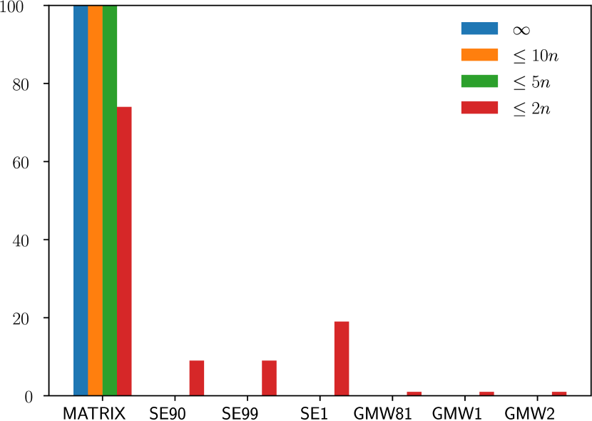
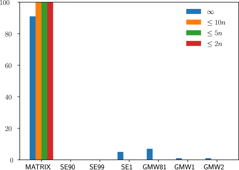
Figure 1: Frequency, how often the algorithm achieved the smallest approximation error for the four different bounds on the condition number of the approximation (different colors) and for each of the six test scenarios (different plots).

The last three scenarios are randomly generated symmetric matrices with eigenvalues uniformly distributed in $[-10^{4},10^{4}]$, $[-10^{4},1]$ or $[-1,10^{4}]$, depending on the scenario, which should be approximated by symmetric positive semidefinite matrices. Each of these random symmetric matrices has been generated by multiplying a random orthogonal matrix, generated with the algorithm described in Stewart1980 , with a diagonal matrix with the chosen eigenvalues as diagonal values and then multiplying this with the transposed random orthogonal matrix. The eigenvalues have been drawn from uniform distributions and were altered so that each matrix has at least one negative and one positive eigenvalue.

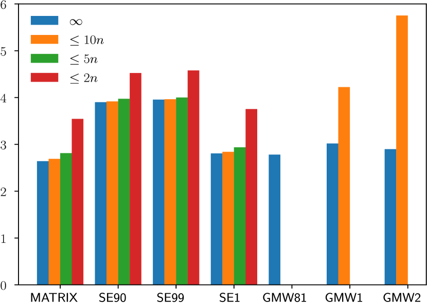
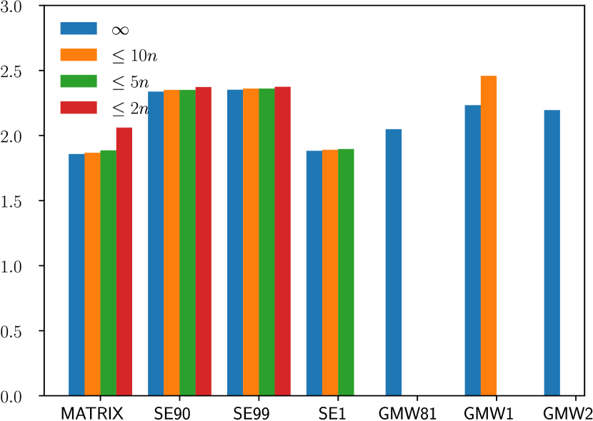
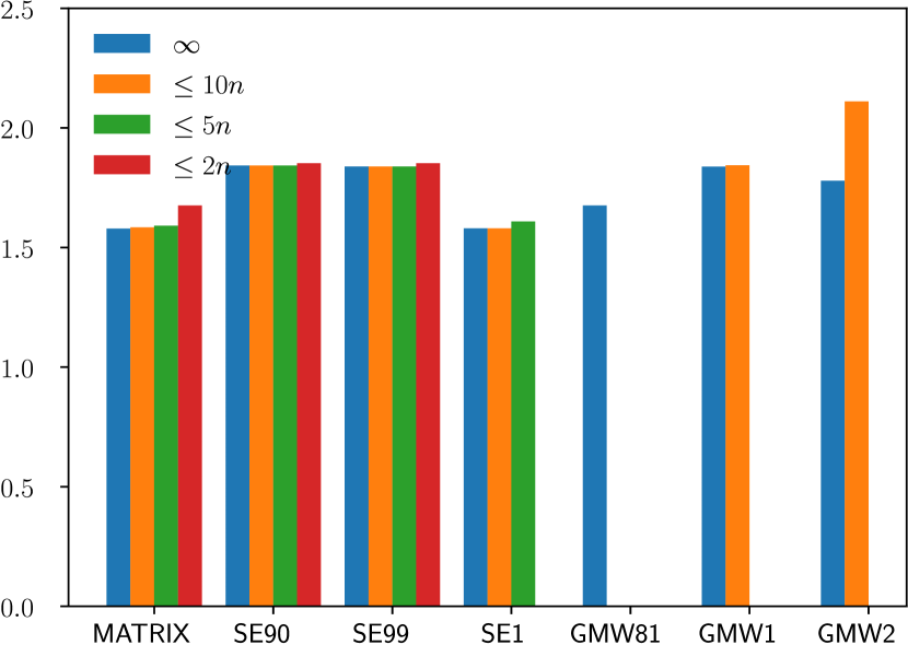
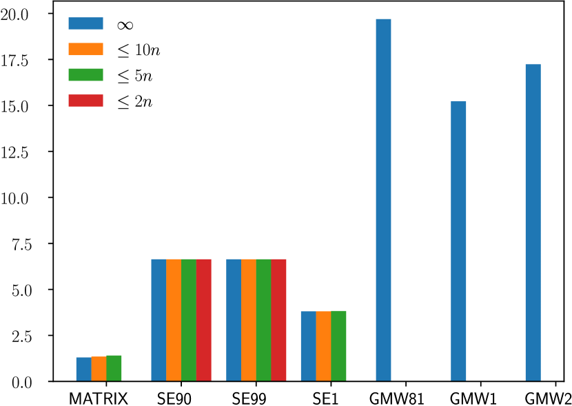
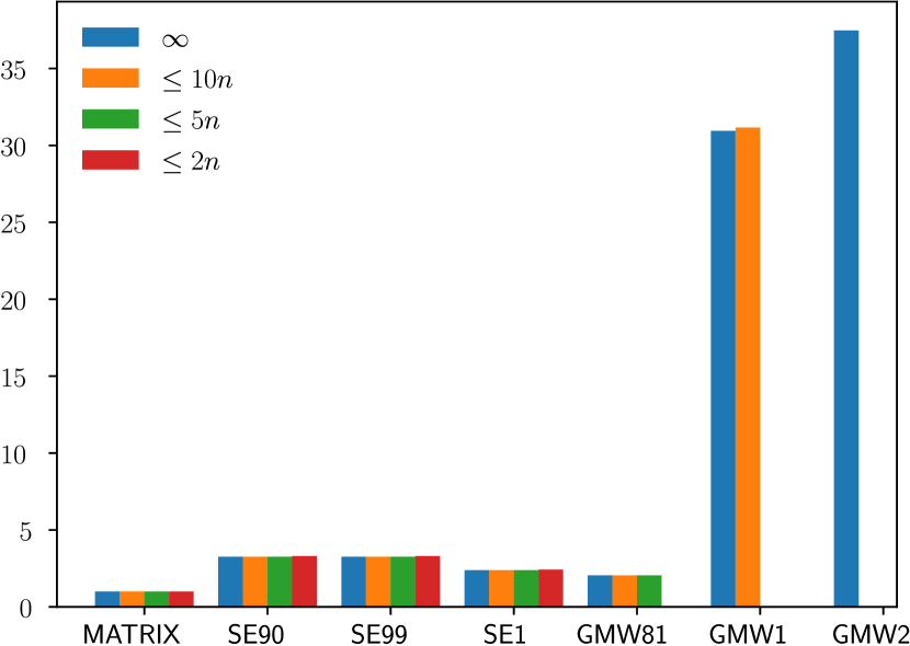
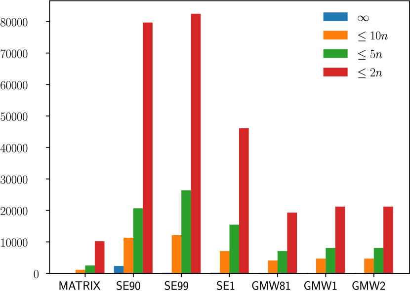
Figure 2: Median of the approximation errors for the four different bounds on the condition number of the approximation (different colors) and for each of the six test scenarios (different plots).

For each of the six scenarios, 100 matrices have been generated with dimensions evenly distributed between 10, 20, 30, 40 and 50 and each of them was approximated.

The approximations are assessed according to the approximation error and their condition number using different objectives. The first one is to minimize the approximation error without caring about the condition number. The other three are to minimize the approximation error while getting a condition number lower or equal to $10n$, $5n$ and $2n$, respectively, where $n$ is the dimension of the matrix. This corresponds to the requirement, that the condition number should be sufficiently small (but must not be minimal), which often occurs in application examples. Minimizing only the condition number without taking the approximation error into account is not useful.

Each of the algorithms has a parameter, representing a lower bound on the values of $D$, allowing to favor a low approximation error or a low condition number. Hence, each algorithm has been executed several times with different values for this parameter and for each of the four objectives only the approximation which best meets the objective was taken into account.

Figure 1 shows how many times each algorithm has computed the approximation with the smallest approximation error among all tested algorithms for the six scenarios and the four objectives. The MATRIX algorithm clearly outperforms all other tested algorithms in all scenarios.

Figure 2 shows the median of the approximation errors for each of the six scenarios and the four objectives. The approximation errors are relative to the minimal possible approximation errors which have been calculated using the methods described in Higham1988 and Higham2002a . No bar in Figure 2 indicates that the algorithm was not able to calculate an approximation with the restriction to the condition number for at least half of the test matrices.

The results show that MATRIX calculates approximations with approximation errors usually close to optimal and still sufficiently small condition numbers. In addition, it performs better, sometimes very considerably, than the other tested algorithms.

The numerical tests have also indicated that, for determining $d_{i}$, a varying lower bound $\hat{l}_{i}$, defined as

$$\hat{l}_{i}:=\begin{cases}l&\text{ if }\tfrac{1}{2}c_{p_{i}}<l\\ u&\text{ if }\tfrac{1}{2}c_{p_{i}}>u\\ \tfrac{1}{2}c_{p_{i}}&\text{ else}\end{cases}\text{ with }c_{i}:=\begin{cases}x_{i}&\text{ if }A_{ii}<x_{i}\\ y_{i}&\text{ if }A_{ii}>y_{i}\\ A_{ii}&\text{ else}\end{cases}$$

for each $i\in\{1\ldots,n\}$, is useful in order to achieve a low approximation error and a low condition number. This varying lower bound is also choosable in the matrix-decomposition library.

4 Conclusions

A new algorithm to approximate Hermitian matrices by positive semidefinite Hermitian matrices was presented. In contrast to existing algorithms, it allows to specify bounds on the diagonal values of the approximation.

It tries to minimize the approximation error in the Frobenius norm and the condition number of the approximation. Parameters of the algorithm can be used to select which of these two objectives is preferred if not both objectives can be meet equally well. Numerical tests have shown that the algorithms outperforms existing algorithms regarding the approximation error as well as the condition number.

The algorithm is suitable for very large matrices, since it needs only $\tfrac{1}{3}n^{3}+\mathcal{O}(n^{2})$ basic operations and storage for $n^{2}+\mathcal{O}(n)$ numbers in the real valued case. This is asymptotically the same number of basic operations as the computation of a Cholesky decomposition would need. Moreover the algorithm is also suitable for sparse matrices since it preserves the sparsity pattern of the original matrix.

The $LDL^{H}$ decomposition of the approximation is calculated as a byproduct. This allows to solve corresponding linear equations or to calculate the corresponding determinant very quickly. If such a decomposition should be calculated anyway, the algorithm has no significant overhead.

Two parts in the algorithm are realizable in many different ways. Various possibilities were presented, more are conceivable.

An open-source implementation of this algorithm is freely available. The implementation is fully documented and easy to install. Extensive numerical tests confirm the functionality of the algorithm and its implementation.

Numerical optimization and statistics are two fields of application in which the algorithm can be of particular interest.

Appendix A Appendix

Theorem A.1

Let $A\in\mathbb{C}^{n\times n}$ be a positive semidefinite matrix. $A$ has a $LDL^{H}$ decomposition. If $A$ is positive definite this decomposition is unique.

Proof

See (Householder1964, , p. 13).

Theorem A.2

Let $L\in\mathbb{C}^{n\times n}$ be a lower triangular matrix with ones on the diagonal and $D\in\mathbb{R}^{n\times n}$ a diagonal matrix. $LDL^{H}$ is

1. invertible if and only if $D_{ii}\neq 0$ for all $i\in\{1,\ldots,n\}$.

2. positive semidefinite if and only if $D_{ii}\geq 0$ for all $i\in\{1,\ldots,n\}$

3. positive definite if and only if $D_{ii}>0$ for all $i\in\{1,\ldots,n\}$.

Proof

Sylvester’s law of inertia Sylvester1852 extended to Hermitian matrices Ikramov2001 implies that $LDL^{H}$ and $D$ have the same number of negative, zero, and respectively positive eigenvalues. Since $D$ is a diagonal matrix, the eigenvalues of $D$ are its diagonal values. Hence $LDL^{H}$ is invertible, positive semidefinite or positive definite if and only if the diagonal values of $D$ are non-zero, non-negative or positive, respectively.

Theorem A.3

Let $A\in\mathbb{C}^{n\times n}$ be a positive definite matrix. Let $L$ and $D$ be the matrices of its $LDL^{H}$ decomposition. Then

$$\left(\frac{\operatorname{trace}(A)}{n\beta}\right)^{\frac{n}{2(n-1)}}\leq\kappa_{2}(L)\leq 2\left(\frac{\operatorname{trace}(A)}{n\alpha}\right)^{\frac{n}{2}},$$

$$\kappa_{2}(D)=\frac{\beta}{\alpha}\text{ and }\kappa_{2}(A)\leq 4\frac{\beta}{\alpha}\left(\frac{\operatorname{trace}(A)}{n\alpha}\right)^{n}$$

$$\text{with }\alpha:=\min_{i=1,\ldots,n}D_{ii}\text{ and }\beta:=\max_{i=1,\ldots,n}D_{ii}.$$

Proof

Define $B:=LL^{H}$. The definition of $B$ implies

$$\kappa_{2}(L)=\sqrt{\kappa_{2}(B)}$$

since $\kappa_{2}(B)=\kappa_{2}(LL^{H})=\kappa_{2}(L)^{2}$.

$L$ is a lower triangular matrix with ones on the diagonal. Hence, $\det(L)=1$ and

$$\det(B)=\det(L)\det(L^{H})=\det(L)^{2}=1.$$

Thus, Davis1961 state that

$$c^{-\frac{1}{n-1}}\leq\kappa_{2}(B)\leq\frac{1+\sqrt{1-c}}{1-\sqrt{1-c}}\text{ ~{}with~{} }c:=\left(\frac{n}{\operatorname{trace}(B)}\right)^{n}.$$ (14)

Besides,

$$\operatorname{trace}(B)=\operatorname{trace}(LL^{H})=\sum\limits_{i,j=1}^{n}L_{ij}\overline{L_{ij}}=\sum\limits_{i,j=1}^{n}|L_{ij}|^{2}=\|L\|_{F}^{2}.$$ (15)

and

$$\|L\|_{F}^{2}=\sum\limits_{i,j=1}^{n}|L_{ij}|^{2}\geq\sum\limits_{i=1}^{n}|L_{ii}|^{2}=n.$$

Hence $0\leq c\leq 1$, which implies

$$\frac{1+\sqrt{1-c}}{1-\sqrt{1-c}}=\frac{(1+\sqrt{1-c})^{2}}{(1-\sqrt{1-c})(1+\sqrt{1-c})}=\frac{(1+\sqrt{1-c})^{2}}{c}\leq\frac{2^{2}}{c}.$$ (16)

Equation (14), (15) and (16) result in

$$\left(\frac{\|L\|_{F}^{2}}{n}\right)^{\frac{n}{n-1}}\leq\kappa_{2}(B)\leq 4\left(\frac{\|L\|_{F}^{2}}{n}\right)^{n}$$

and thus

$$\left(\frac{\|L\|_{F}^{2}}{n}\right)^{\frac{n}{2(n-1)}}\leq\kappa_{2}(L)\leq 2\left(\frac{\|L\|_{F}^{2}}{n}\right)^{\frac{n}{2}}.$$ (17)

Theorem A.2 implies $0<\alpha$ because $A$ is positive definite. Moreover, $\alpha\leq D_{ii}\leq\beta$ for all $i\in\{1,\ldots,n\}$ by definition of $\alpha$ and $\beta$. Thus

$$\frac{\operatorname{trace}(A)}{\beta} =\frac{1}{\beta}\sum\limits_{i=1}^{n}A_{ii}=\frac{1}{\beta}\sum\limits_{i=1}^{n}\sum\limits_{j=1}^{n}L_{ij}D_{jj}\overline{L}_{ij}=\sum\limits_{i=1}^{n}\sum\limits_{j=1}^{n}|L_{ij}|^{2}\frac{D_{jj}}{\beta}$$

$$\leq\sum\limits_{i=1}^{n}\sum\limits_{j=1}^{n}|L_{ij}|^{2}=\|L\|_{F}^{2}=\sum\limits_{i=1}^{n}\sum\limits_{j=1}^{n}|L_{ij}|^{2}$$

$$\leq\sum\limits_{i=1}^{n}\sum\limits_{j=1}^{n}|L_{ij}|^{2}\frac{D_{jj}}{\alpha}=\frac{1}{\alpha}\sum\limits_{i=1}^{n}\sum\limits_{j=1}^{n}L_{ij}D_{jj}\overline{L}_{ij}=\frac{1}{\alpha}\sum\limits_{i=1}^{n}A_{ii}=\frac{\operatorname{trace}(A)}{\alpha}.$$

Hence

$$\left(\frac{\operatorname{trace}(A)}{n\beta}\right)^{\frac{n}{2(n-1)}}\leq\kappa_{2}(L)\leq 2\left(\frac{\operatorname{trace}(A)}{n\alpha}\right)^{\frac{n}{2}}$$

with (17).

Furthermore

$$\kappa_{2}(D)=\frac{\max\limits_{i=1,\ldots,n}|D_{ii}|}{\min\limits_{i=1,\ldots,n}|D_{ii}|}=\frac{\beta}{\alpha}$$

since $D$ is a diagonal matrix. Thus

$$\kappa_{2}(A) =\kappa_{2}(LDL^{H})\leq\kappa_{2}(L)\kappa_{2}(D)\kappa_{2}(L^{H})$$

$$=\kappa_{2}(L)^{2}\kappa_{2}(D)\leq 4\frac{\beta}{\alpha}\left(\frac{\|L\|_{F}^{2}}{n}\right)^{n},$$

because $\kappa_{2}(AB)\leq\kappa_{2}(A)\kappa_{2}(B)$ and $\kappa_{2}(A)=\kappa_{2}(A^{H})$ for every invertible matrices $A,B\in\mathbb{C}^{n\times n}$.

References

• (1) Amestoy, P.R., Davis, T.A., Duff, I.S.: An Approximate Minimum Degree Ordering Algorithm. SIAM Journal on Matrix Analysis and Applications 17(4), 886–905 (1996). DOI 10.1137/S0895479894278952
• (2) Anaconda, I.: Conda Package Manager. URL https://conda.io/docs/index.html
• (3) Borsdorf, R., Higham, N.J.: A Preconditioned Newton Algorithm for the Nearest Correlation Matrix. IMA J. Numer. Anal. 30(1), 94–107 (2010). DOI 10.1093/imanum/drn085
• (4) Borsdorf, R., Higham, N.J., Raydan, M.: Computing a Nearest Correlation Matrix with Factor Structure. SIAM J. Matrix Anal. Appl. 31(5), 2603–2622 (2010). DOI 10.1137/090776718
• (5) Brandl, G., et al.: Sphinx: Python documentation generator (2019). URL www.sphinx-doc.org. Version 2.0.1
• (6) Chen, Y., Wiesel, A., Eldar, Y.C., Hero, A.O.: Shrinkage Algorithms for MMSE Covariance Estimation. IEEE Transactions on Signal Processing 58(10), 5016–5029 (2010). DOI 10.1109/TSP.2010.2053029
• (7) Cheng, S., Higham, N.: A Modified Cholesky Algorithm Based on a Symmetric Indefinite Factorization. SIAM Journal on Matrix Analysis and Applications 19(4), 1097–1110 (1998). DOI 10.1137/S0895479896302898
• (8) Chong, E., Zak, S.: An Introduction to Optimization, 4th edn. Wiley Series in Discrete Mathematics and Optimization. Wiley (2013)
• (9) Cuthill, E., McKee, J.: Reducing the Bandwidth of Sparse Symmetric Matrices. In: Proceedings of the 1969 24th National Conference, ACM ’69, pp. 157–172. ACM, New York, NY, USA (1969). DOI 10.1145/800195.805928
• (10) Davies, P.I., Higham, N.J.: Numerically Stable Generation of Correlation Matrices and Their Factors. BIT Numerical Mathematics 40(4), 640–651 (2000). DOI 10.1023/A:1022384216930. URL https://doi.org/10.1023/A:1022384216930
• (11) Davis, P.J., Haynsworth, E.V., Marcus, M.: Bound for the P-condition number of matrices with positive roots. J. Res. Natl. Bur. Stand. B 65, 13–14 (1961)
• (12) Davis, T.: Direct Methods for Sparse Linear Systems. Society for Industrial and Applied Mathematics (2006). DOI 10.1137/1.9780898718881
• (13) Davis, T.A., Rajamanickam, S., Sid-Lakhdar, W.M.: A survey of direct methods for sparse linear systems. Acta Numerica 25, 383–566 (2016). DOI 10.1017/S0962492916000076
• (14) Devlin, S.J., Gnanadesikan, R., Kettenring, J.R.: Robust estimation and outlier detection with correlation coefficients. Biometrika 62(3), 531–545 (1975)
• (15) Fang, H.r., O’Leary, D.P.: Modified Cholesky algorithms: a catalog with new approaches. Mathematical Programming 115(2), 319–349 (2008). DOI 10.1007/s10107-007-0177-6
• (16) Fisher, T.J., Sun, X.: Improved Stein-type shrinkage estimators for the high-dimensional multivariate normal covariance matrix. Computational Statistics & Data Analysis 55(5), 1909–1918 (2011). DOI 10.1016/j.csda.2010.12.006. URL http://www.sciencedirect.com/science/article/pii/S0167947310004743
• (17) George, A., Liu, J.W.: Computer Solution of Large Sparse Positive Definite. Prentice Hall Professional Technical Reference (1981)
• (18) George, A., Liu, J.W.: The Evolution of the Minimum Degree Ordering Algorithm. SIAM Review 31(1), 1–19 (1989). DOI 10.1137/1031001
• (19) Gill, P.E., Murray, W.: Newton-type methods for unconstrained and linearly constrained optimization. Mathematical Programming 7(1), 311–350 (1974). DOI 10.1007/BF01585529
• (20) Gill, P.E., Murray, W., Wright, M.H.: Practical optimization. Academic press (1981)
• (21) Goldfeld, S.M., Quandt, R.E., Trotter, H.F.: Maximization by Quadratic Hill-Climbing. Econometrica 34(3), 541–551 (1966)
• (22) Golub, G.H., Van Loan, C.F.: Matrix Computations, third edn. The Johns Hopkins University Press, Baltimore, MD, USA (1996)
• (23) Higham, N., Strabić, N., Šego, V.: Restoring Definiteness via Shrinking, with an Application to Correlation Matrices with a Fixed Block. SIAM Review 58(2), 245–263 (2016). DOI 10.1137/140996112. URL https://doi.org/10.1137/140996112
• (24) Higham, N.J.: Computing a nearest symmetric positive semidefinite matrix. Linear Algebra and its Applications 103, 103–118 (1988). DOI 10.1016/0024-3795(88)90223-6. URL http://www.sciencedirect.com/science/article/pii/0024379588902236
• (25) Higham, N.J.: Matrix Nearness Problems and Applications. In: M.J.C. Gover, S. Barnett (eds.) Applications of Matrix Theory, pp. 1–27. Oxford University Press (1989)
• (26) Higham, N.J.: Accuracy and Stability of Numerical Algorithms, 2nd edn. Society for Industrial and Applied Mathematics, Philadelphia, PA, USA (2002). DOI 10.1137/1.9780898718027
• (27) Higham, N.J.: Computing the Nearest Correlation Matrix - A Problem from Finance. IMA J. Numer. Anal. 22(3), 329–343 (2002). DOI 10.1093/imanum/22.3.329
• (28) Higham, N.J., Strabić, N.: Anderson Acceleration of the Alternating Projections Method for Computing the Nearest Correlation Matrix. Numerical Algorithms 72(4), 1021–1042 (2016). DOI 10.1007/s11075-015-0078-3. URL https://doi.org/10.1007/s11075-015-0078-3
• (29) Householder, A.S.: The theory of matrices in numerical analysis. Blaisdell Publishing Company (1964)
• (30) Ikeda, Y., Kubokawa, T., Srivastava, M.S.: Comparison of linear shrinkage estimators of a large covariance matrix in normal and non-normal distributions. Computational Statistics & Data Analysis 95, 95–108 (2016). DOI 10.1016/j.csda.2015.09.011. URL http://www.sciencedirect.com/science/article/pii/S0167947315002388
• (31) Ikramov, K.D.: On the inertia law for normal matrices. In: Doklady Mathematics C/C of Doklady Akademii Nauk, vol. 64, pp. 141–142 (2001)
• (32) Iman, R., Davenport, J.: An iterative algorithm to produce a positive definite correlation matrix from an approximate correlation matrix (with a program user’s guide). Tech. rep., Sandia National Labs., Albuquerque, NM (USA) (1982). DOI 10.2172/5152227. URL https://doi.org/10.2172/5152227
• (33) Jones, E., Oliphant, T., Peterson, P., et al.: SciPy: library for scientific computing with Python (2019). URL http://www.scipy.org. Version 1.3
• (34) Krekel, H., et al.: pytest: helps you write better programs (2019). URL https://docs.pytest.or. Version 4.4.1
• (35) Ledoit, O., Wolf, M.: Improved estimation of the covariance matrix of stock returns with an application to portfolio selection. Journal of Empirical Finance 10(5), 603–621 (2003). DOI 10.1016/S0927-5398(03)00007-0. URL http://www.sciencedirect.com/science/article/pii/S0927539803000070
• (36) Ledoit, O., Wolf, M.: A well-conditioned estimator for large-dimensional covariance matrices. Journal of Multivariate Analysis 88(2), 365–411 (2004). DOI 10.1016/S0047-259X(03)00096-4. URL http://www.sciencedirect.com/science/article/pii/S0047259X03000964
• (37) Levenberg, K.: A method for the solution of certain problems in least squares. Quarterly of applied mathematics 2(2), 164–168 (1944)
• (38) Marquardt, D.W.: An Algorithm for Least-Squares Estimation of Nonlinear Parameters. Journal of the Society for Industrial and Applied Mathematics 11(2), 431–441 (1963). URL http://www.jstor.org/stable/2098941
• (39) Moré, J.J., Sorensen, D.C.: On the use of directions of negative curvature in a modified newton method. Mathematical Programming 16(1), 1–20 (1979). DOI 10.1007/BF01582091. URL https://doi.org/10.1007/BF01582091
• (40) Nocedal, J., Wright, S.: Numerical Optimization, second edn. Springer series in operations research and financial engineering. Springer, New York (2006)
• (41) Oliphant, T.E., et al.: NumPy: N-dimensional array package for Python (2019). URL http://www.numpy.org. Version 1.17
• (42) PyPA: The Python Package Installer. URL https://pip.pypa.io
• (43) Python Software Foundation: Python (2018). URL http://www.python.org. Version 3.7
• (44) Qi, H., Sun, D.: Correlation stress testing for value-at-risk: an unconstrained convex optimization approach. Computational Optimization and Applications 45(2), 427–462 (2010). DOI 10.1007/s10589-008-9231-4. URL https://doi.org/10.1007/s10589-008-9231-4
• (45) Reimer, J.: Conda package for matrix-decomposition: a library for decompose (factorize) dense and sparse matrices in Python. URL https://anaconda.org/jore/matrix-decomposition
• (46) Reimer, J.: GitHub repository for matrix-decomposition: a library for decompose (factorize) dense and sparse matrices in Python. https://github.com/jor-/matrix-decomposition. URL https://github.com/jor-/matrix-decomposition
• (47) Reimer, J.: Python package for matrix-decomposition: a library for decompose (factorize) dense and sparse matrices in Python. URL https://pypi.org/project/matrix-decomposition/
• (48) Reimer, J.: matrix-decomposition: a library for decompose (factorize) dense and sparse matrices in Python (2019). DOI 10.5281/zenodo.3558540. URL https://doi.org/10.5281/zenodo.3558540. Version 1.2
• (49) Reimer, J., Grigorievskiy, A., Lee, A., Yuri, Barrett, L., Seljebotn, D.S., Smith, N., Cournapeau, D.: scikit-sparse: a library for sparse matrix manipulation in Python (2018). URL https://github.com/scikit-sparse/scikit-sparse. Version 0.4.4
• (50) Rousseeuw, P.J., Molenberghs, G.: Transformation of non positive semidefinite correlation matrices. Communications in Statistics–Theory and Methods 22(4), 965–984 (1993)
• (51) Rudin, W.: Principles of Mathematical Analysis. International series in pure and applied mathematics. McGraw-Hill (1976)
• (52) Schäfer, J., Strimmer, K.: A Shrinkage Approach to Large-Scale Covariance Matrix Estimation and Implications for Functional Genomics. Statistical Applications in Genetics and Molecular Biology 4(1), 1–32 (2005)
• (53) Schnabel, R., Eskow, E.: A New Modified Cholesky Factorization. SIAM Journal on Scientific and Statistical Computing 11(6), 1136–1158 (1990). DOI 10.1137/0911064
• (54) Schnabel, R., Eskow, E.: A Revised Modified Cholesky Factorization Algorithm. SIAM Journal on Optimization 9(4), 1135–1148 (1999). DOI 10.1137/S105262349833266X
• (55) Stein, C.: Inadmissibility of the Usual Estimator for the Mean of a Multivariate Normal Distribution. In: Proceedings of the Third Berkeley Symposium on Mathematical Statistics and Probability, Volume 1: Contributions to the Theory of Statistics, pp. 197–206. University of California Press, Berkeley, Calif. (1956)
• (56) Stewart, G.: The Efficient Generation of Random Orthogonal Matrices with an Application to Condition Estimators. SIAM Journal on Numerical Analysis 17(3), 403–409 (1980). DOI 10.1137/0717034. URL https://doi.org/10.1137/0717034
• (57) Sylvester, J.J.: A demonstration of the theorem that every homogeneous quadratic polynomial is reducible by real orthogonal substitutions to the form of a sum of positive and negative squares. The London, Edinburgh, and Dublin Philosophical Magazine and Journal of Science 4(23), 138–142 (1852)
• (58) Touloumis, A.: Nonparametric Stein-type shrinkage covariance matrix estimators in high-dimensional settings. Computational Statistics & Data Analysis 83, 251–261 (2015). DOI 10.1016/j.csda.2014.10.018. URL http://www.sciencedirect.com/science/article/pii/S0167947314003107
• (59) Virtanen, P., Gommers, R., Oliphant, T.E., Haberland, M., Reddy, T., Cournapeau, D., Burovski, E., Peterson, P., Weckesser, W., Bright, J., van der Walt, S., Brett, M., Wilson, J., Millman, K.J., Mayorov, N., Nelson, A.R.J., Jones, E., Kern, R., Larson, E., Carey, C.J., Polat, I., Feng, Y., Moore, E.W., VanderPlas, J., Laxalde, D., Perktold, J., Cimrman, R., Henriksen, I., Quintero, E.A., Harris, C.R., Archibald, A.M., Ribeiro, A.H., Pedregosa, F., van Mulbregt, P., SciPy: SciPy 1.0-Fundamental Algorithms for Scientific Computing in Python. CoRR abs/1907.10121 (2019). URL http://arxiv.org/abs/1907.10121
• (60) Yannakakis, M.: Computing the Minimum Fill-In is NP-Complete. SIAM Journal on Algebraic Discrete Methods 2(1), 77–79 (1981). DOI 10.1137/0602010