Thermal conductance of zero modes on the surface boundary of a Weyl semimetal

Abstract

Thermoelectric conductance of Dirac materials and in particular zero modes reveals the effect of topology .Weyl semimetals with a boundary at $z=0$ give rise to chiral zero modes without backscattering resulting in a significant contribution to thermal conductivity. By doping the surface with paramagnetic impurities backscattering is allowed, and the thermal conductivity is controlled by the decrease of the transmission function $|t|^{2}<1$ . We attach a thermal reservoir at the edge of the sample and study the thermal and electrical conductance. For the ballistic and mesoscopic situations, quantum fluctuations causes oscillations of the thermal and electric conductance. The thermoelectric conductance varies periodically with the voltage bias. We compare the thermal conductance with and without impurity scattering and observe the effects of topology. An experimental set-up is proposed to test this theory.

I. INTRODUCTION

Thermal conductance is the flow of heat that results from a temperature gradientMahan . Thermoelectrics are used in cooler refrigerators based on the Peltier Goldsmith effect which predicts the appearance of a heat current when an electric current passes through a material. Alternatively, the Seebeck effect generates an electric current from a temperature gradient Kamran . According to Mahan , the presence of a disorder can might enhance the figure of merit Kamran . These results have been obtained within the semiclassical Boltzmann theory. Recent experiment performed by Pepper suggest that interference effects are important and may invalidate the Boltzmann theory. It was shown that edge states affect the thermal cconductance Banerjee .

Another situation where edge modes contribute to the thermal conductance are surface zero modes of Weyl semimetals David .The Weyl semimetals are topological materials that are protected against localization. The disordered Weyl semimetals resemble a three dimensional Anderson metal Altland . In agreement with this we find that the boundary surface support zero modes . As a function of the surface width in the $x$ direction we find $2N$ chiral modes which propagate in the $y$ direction. Due to topology the chiral modes are protected against backscattering and the thermal conductance is given by $\kappa=2N\frac{\pi^{2}K^{2}_{B}T}{3h}$ with the value of $N$ being determinate by the temperatur. Doping the Weyl surface with paramagnetic impurities generates a system of $2N$ chiral backscattering pairs. The computation is done by the applying Landau Buttiker theory Buttiker ; Flensberg to Dirac materials with particles and anti-particles. We obtain a system of $N$ one dimensional zero modes where the Landau Buttiker theory Butcher will be applied. We investigate the thermal effects in the temperature range where the electronic systems obey the ballistic or the mesoscopic conditions. We find that the thermoelectric conductance fluctuates strongly with the change of the chemical potential . This result is in agreement with the fluctuations controlled by density change observed by Pepper .

The plan of this paper is outlined as follows:In chapter II we will consider a Weyl semimetal crystal with a boundary at $z=0$. As a result, zero modes lie on the two dimensional boundary at $z=0$.In section III we show that if we restrict the crystal to a width of $D_{x}$ perpendicular to the line which connects the monopole and the anti- monopole we obtain N pairs of chiral zero modes . In chapter IV we consider the Landauer Buttiker formulation for Dirac fermions with the perfect transmission $|t|^{2}=1$ and compute the electric conductance $G$,thermoelectric conductance $L$ and thermal conductance $\kappa$ at finite temperatures for the ballistic condition. In chapter V, we include magnetic impurities which give rise to backscattering with non perfect transmission, $|t|^{2}<1$ allowing to investigate the mesoscopic conditions In chapter VI, we propose an experimental set-up for testing th theory. In section VII we present our conclusion.

II. The Weyl Hamiltonian with a boundary at $z=0$, confined to the crystal region $-L\leq z\leq 0$

The bulk of the Weyl semimetals ( $WSMs$) is dominated by Weyl points and linear, low energy excitation. The Weyl points come in pairs with opposite chirality Ninomya . The surface state of the $WSMs$ is characterized by ${}^{{}^{\prime\prime}}$Fermi arcs${}^{{}^{\prime\prime}}$ that link the projection of the bulk Weyl points in the Brillouine zone. The $WSMs$ exist in materials where time-reversal symmetry or inversion are broken. Recently, the non-centrosymmetric and non-crystal magnetic transition-metal monoarsenide/posphides $TaAs$ ,$TaP$, $NbAs$ and $NbP$ have been predicted to be $WSMs$ with $12$ pairs of Weyl points Science . We consider a $WSM$ Hamiltonian which describes fermions with opposite chirality and two singularities at $k_{x}=\pm M$. A $WSM$ model without a boundary and two nodes $\vec{M}=[\pm M,0,0]$ is given by the Hamiltonian:

$$\tilde{H}=\int\,d^{3}x\hbar v\Big{[}\hat{\Psi}^{\dagger}_{R}(\vec{x})\vec{\sigma}\cdot\Big{(}-i\vec{\partial}-\vec{M}\Big{)}\hat{\Psi}_{R}(\vec{x})-\hat{\Psi}^{\dagger}_{L}(\vec{x})\vec{\sigma}\cdot\Big{(}-i\vec{\partial}-(-\vec{M})\Big{)}\hat{\Psi}_{L}(\vec{x})\Big{]}$$ (1)

This model is oversimplified and does not include the band dispersion which connects the two nodes. In order to observe this connection, we need to study a model with two non-linearly dispersed bands. We are guided by the fact that the singularities at $k_{x}=\pm M$ describe a monopole and anti-monopole . To describe the crossing of the bands in momentum space, we will introduce a quadratic function of momentum $g(k^{2}_{x}-M^{2})$ which reproduces the nodes at $\pm M$ ( this polynomial is obtained by replacing $-cos(k_{x})+1\approx\frac{k^{2}_{x}}{2}$) for the two band Hamiltonian $\hat{h}(\vec{k},z)$: $\hat{h}(\vec{k},z)=\hbar v\Big{[}\sigma_{y}\tau_{3}k_{y}+\sigma_{z}\tau_{3}k_{z}+\sigma_{y}\tau_{2}g(k^{2}_{x}-M^{2})\Big{]}$. The Hamiltonian with the boundary at $z=0$ and potential energy $\hbar vk_{0}$ is given by:

$$H=\int\frac{d^{2}k}{(2\pi)^{2}}\int_{-L}^{0}\,dz\Big{[}\hbar v\hat{\Psi}^{\dagger}(\vec{k},z)h(\vec{k},z)\hat{\Psi}(\vec{k},z)\Big{]};h(\vec{k},z)=h^{(0)}(\vec{k},z)+h^{(1)};(\vec{k})$$

$$h^{(0)}(\vec{k},z)=\Big{(}\sigma_{z}\tau_{3}(-i\partial_{z})+\sigma_{y}\tau_{2}g(k^{2}_{x}-M^{2})\Big{)}\hskip 7.22743pt;h^{(1)}(\vec{k})=\Big{(}\sigma_{y}\tau_{3}k_{y}-k_{0}I\Big{)}$$

with the zero modes solution, $h^{(0)}(\vec{k},z)U_{i=1,2}(\vec{k},z)=EU_{i=1,2}(\vec{k},z)$.

$$U(\vec{k},z)=e^{\lambda z}V(\vec{k})=\sum_{s=\pm}\Big{[}\theta[k^{2}_{x}-M^{2}]e^{g(k^{2}_{x}-M^{2})z}\eta_{i,+;s}+\theta[-k^{2}_{x}+M^{2}]e^{-g(-k^{2}_{x}+M^{2})z}\eta_{i,-;s}(\vec{k})\Big{]};\vspace{0.05 in}k^{2}\neq M^{2}$$ (3)

We mention that in addition to the zero modes $E=0$ we have non-zero modes excitations. At low temperatures, we can neglect the nonzero modes. Therefore for temperatures $T<T_{M}$ we ignore the non zero modes. The probability for exciting non zero modes on the surface is $f_{f.D.n\neq 0}=(1+e^{\frac{\hbar v\sqrt{k^{2}_{y}+k^{2}_{x}}-\hbar vk_{0}}{K_{B}T}})^{-1}$ and the probablity for exciting zero modes is $f_{f.D.n=0}=(1+e^{\frac{\hbar v|k_{y}|-\hbar vk_{0}}{K_{B}T}})^{-1}$. At low temperatures we have , $f_{f.D.n\neq 0}<<f_{f.D.n=0}$.

According to Witten , we identify the zero modes with boundary surface states at $z=0$. The zero mode solutions $\eta_{i,\pm;s}$, $i=1,2$ with the index $\pm$ refering to the momentum region $k^{2}_{x}>M^{2}$ or $M^{2}>k^{2}_{x}$ while $s$ refers to $\pm k_{x}$ David .

$$\eta_{1,+;s}=\sqrt{\frac{1}{2}}\Big{[}i,0,0,1\Big{]}^{T},\hskip 3.61371pt\eta_{1,-;s}=\sqrt{\frac{1}{2}}\Big{[}-i,0,0,1\Big{]}^{T}$$

$$\eta_{2,+;s}=\sqrt{\frac{1}{2}}\Big{[}0,i,1,0\Big{]}^{T},\hskip 3.61371pt\eta_{2,-;s}=\sqrt{\frac{1}{2}}\Big{[}0,-i,1,0\Big{]}^{T}$$

Following David we diagonalyze $h^{(1)}(\vec{k})$ in terms of the zero modes operators $C_{1,-;s}$, $C_{2,-;s}$, $C_{1,+;s}$, $C_{2,+;s}$ .

$$H^{\perp}=\int\frac{dk_{y}}{(2\pi)}\sum_{k_{x}}\sum_{\pm}\Big{[}\hbar v\Big{[}k_{y}\Big{(}-iC^{\dagger}_{1,-;s}(\vec{k})C_{2-;s}(\vec{k})+iC^{\dagger}_{2-;s,}(\vec{k})C_{1-;,s}(\vec{k})\Big{)}$$

$$-k_{0}\Big{(}C^{\dagger}_{1,-;s}(\vec{k})C_{1,-;,s}(\vec{k})+C^{\dagger}_{2,-;s}(\vec{k})C_{2,-;s}(\vec{k})\Big{)}\Big{]}\theta[k^{2}_{x}-M^{2}]$$

$$+\hbar v\Big{[}k_{y}\Big{(}-iC^{\dagger}_{1,+;s}(\vec{k})C_{2,+;s}(\vec{k})+iC^{\dagger}_{2,+;s,}(\vec{k})C_{1,+;,s}(\vec{k})\Big{)}$$

$$-k_{0}\Big{(}C^{\dagger}_{1,+;s}(\vec{k})C_{1,+;,s}(\vec{k})+C^{\dagger}_{2,+;s}(\vec{k})C_{2,+;s}(\vec{k})\Big{)}\Big{]}\theta[-k^{2}_{x}+M^{2}]\Big{]}$$

We replace the operator $C_{1,-;s}$, $C_{2,-;s}$, $C_{1,+;s}$, $C_{2,+;s}$ with the eigenvalue operators, $C_{\pm,\pm;s}$. We have the transformation : $C_{1,-;s}=\frac{1}{\sqrt{2}}(C_{+,-;s}+C_{-,-;s})$ , $C_{1,+;s}=\frac{1}{\sqrt{2}}(C_{+,+;s}+C_{-,+;s})$ $C_{2,-;s}=\frac{i}{\sqrt{2}}(C_{+,-;s}-C_{-,-;s})$ ,$C_{2,+;s}=\frac{1}{\sqrt{2}}(C_{+,+;s}+C_{-,+;s})$. We replace the spinors $\eta_{i,+;s}$ ,$\eta_{i,-;s}$ $i=1,2$ with transformed spinors $\eta_{\pm,+;s}$, $\eta_{\pm,-;s}$:

$$\eta_{+,-;s}=\frac{1}{\sqrt{2}}[-i,1,i,1],\hskip 0.72229pt\eta_{-,-;s}=\frac{1}{\sqrt{2}}[-i,-1,-i,1];\eta_{+,+;s}=\frac{1}{\sqrt{2}}[i,-1,i,1],\hskip 0.72229pt\eta_{-,+;s}=\frac{1}{\sqrt{2}}[i,1,-i,1]$$ (6)

For a sample of width $D_{x}$, the momentum $k_{x}$ is discreet, $k_{x}=\frac{2\pi}{D_{x}}(n_{x}+\frac{1}{2})$, $n_{x}=\pm 1,\pm 2....$ (see Figure.1) with $n_{x,max.}$ given by $n_{x,max.}=\frac{M}{\frac{2\pi}{D_{x}}}-\frac{1}{2}$ . At finite temperature $T<T_{M}$, we can define $N$ as the number of excited modes in the $x$ direction, $\mathbf{N=\frac{K_{B}T}{\hbar v_{\perp}\frac{2\pi}{D_{x}}}}$ ($\hbar v_{\perp}\frac{2\pi}{D_{x}}$ the excitation energy in the $x$ direction which satisfies the conditions $v_{\perp}<v$) .When $n_{x,max.}$ is larger than the thermal mode excited $N$, we have the representation ( $n_{x,max.}>N$):

$$H^{\perp}=\sum_{s=\pm}\int\,\frac{dk_{y}}{2\pi}\Big{[}\hbar v(k_{y}-k_{0})\Big{(}C^{\dagger}_{+,-;s}(\vec{k})C_{+,-;s}(\vec{k})+C^{\dagger}_{-,-;s}(\vec{k})C_{-,-;s}(\vec{k})\Big{)}$$

$$+\sum_{n_{x}=1}^{N}\sum_{s=\pm}\int\,\frac{dk_{y}}{2\pi}\hbar v(k_{y}-k_{0})\Big{(}C^{\dagger}_{+,-;s,n_{x}}(\vec{k})C_{+,-;s,n_{x}}(\vec{k})+C^{\dagger}_{-,-;s,n_{x}}(\vec{k})C_{-,-;s,n_{x}}(\vec{k})\Big{)}$$

$$+\sum_{n_{x}=N}^{n_{x,max}}\sum_{s=\pm}\int\,\frac{dk_{y}}{2\pi}\hbar v(k_{y}-k_{0})\Big{(}C^{\dagger}_{+,-;s,n_{x}}(\vec{k})C_{+,-;s,n_{x}}(\vec{k})+C^{\dagger}_{-,-;s,n_{x}}(\vec{k})C_{-,-;s,n_{x}}(\vec{k})\Big{)}\Big{]}$$

For the case $n_{x,max.}>N$ we have only modes which obey $k^{2}_{x}>M^{2}$ with spinors $\eta_{+,-;s}$ and $\eta_{-,-;s}$.

In the opposite situation, $n_{x,max.}<N$, we have two type of modes : modes with $k^{2}_{x}>M^{2}$ and modes with $k^{2}_{x}<M^{2}$. For this case, we have both spinors $\eta_{+,+;s}$ , $\eta_{-,+;s}$ see Eq.$3$ and $\eta_{+,-;s}$ , $\eta_{-,-;s}$.

$$H^{\perp}=\sum_{n_{x}=1}^{n_{x,max.}}\sum_{s=\pm}\int\,\frac{dk_{y}}{2\pi}\hbar v(k_{y}-k_{0})\Big{(}C^{\dagger}_{+,-;s,n_{x}}(\vec{k})C_{+,-;s,n_{x}}(\vec{k})+C^{\dagger}_{-,-;s,n_{x}}(\vec{k})C_{-,-;s,n_{x}}(\vec{k})\Big{)}$$

$$+\sum_{n_{x}=n_{x,max.}}^{N}\sum_{s=\pm}\int\,\frac{dk_{y}}{2\pi}\hbar v(k_{y}-k_{0})\Big{(}C^{\dagger}_{+,+;s,n_{x}}(\vec{k})C_{+,+;s,n_{x}}(\vec{k})+C^{\dagger}_{-,+;s,n_{x}}(\vec{k})C_{-,+;s,n_{x}}(\vec{k})\Big{)}$$

For this case we use the spinors $\eta_{+,+;s}$ and $\eta_{-,+;s}$ (see Eq.$3$).

In Figure $1$, we show the one dimensional channels as a function of the discreete momentum $k_{x}$. We observe that for each value of $k_{x}$ , we have left and right fermions. This demonstrates that the surface of Weyl semimetal is equivalent to $N$ pair of chiral fermions (see Figure.1) .

III-The quasi one-dimension edge mode

For a narrow width, $D_{x}$, we can consider only the zero mode at fixed momentum $k_{x}=\pm\frac{\pi}{D_{x}}$ which propagates along the $y$ direction. We have a mode with two chiralities. The $y$ direction needs to be perpendicular to the line connecting the pair of monopole anti-monopole. Thus, we replace $H^{\perp}$ $\rightarrow$ $H^{edge}$. The Hamiltonian at the fixed momentum $k_{x}=\pm\frac{\pi}{D_{x}}$ takes the form:

$$H^{edge}=\sum_{s=\pm}\int\,\frac{dk_{y}}{2\pi}\Big{[}\hbar v(k_{y}-k_{0})C^{\dagger}_{+,-;s}(\vec{k})C_{+,-;s}(\vec{k})+\hbar v(-k_{y}-k_{0})C^{\dagger}_{-,-;s}(\vec{k})C_{-,-;s}(\vec{k})\Big{]}$$ (9)

We represent $C_{+,-;s}(k_{y})$ and $C_{-,-;s}(k_{y})$ in terms of the particle operators $a(k)$ and anti-particle $b^{\dagger}(k)$:The second minus stand for the case that $k^{2}_{x}<M^{2}$ .

$$C_{+,-;s}(k_{y})=a_{+,-;s}(k_{y})\theta[k_{y}]+b^{\dagger}_{+,-;s}(-k_{y})\theta[-k_{y}];\hskip 3.61371ptC_{-,-;s}(k_{y})=a_{-,-;s}(-k_{y})\theta[-k_{y}]+b^{\dagger}_{-,-;s}(k_{y})\theta[k_{y}]$$ (10)

For $0\leq k<\infty$, we introduce $k=q+k_{F}$, and for $-\infty<k\leq 0$, we introduce $k=q-k_{F}$ with $-2k_{F}\leq q\leq 2k_{F}$. We introduce an ultraviolet cut-off $\Lambda$ , $2k_{F}=\frac{\pi}{a}\approx\Lambda$. At half filling $k_{0}=0$, the fermion field is given in terms of the left and right movers : $C_{-,-;s}(y)=e^{-ik_{F}y}\psi_{-,-;s}(y)\eta_{-,-;s}$ , $C_{+,-;s}(y)=e^{ik_{F}y}\psi_{+,-;s}(y)\eta_{+,-;s}$ , where :

$$\psi_{+,-;s}(y)=\int_{-\Lambda}^{\Lambda}\frac{dq}{2\pi}\psi_{+,-;s}(q)\eta_{+,-;s}e^{iqy}\hskip 0.72229pt;\psi_{-,-;s}(y)=\int_{-\Lambda}^{\Lambda}\frac{dq}{2\pi}\psi_{-,-;s}(q)\eta_{-,-;s}e^{-iqy}$$

$$\psi_{+,-;s}(q)=\alpha_{+,-;s}(q)\theta[q]+\beta^{\dagger}_{+,-;s}(-q)\theta[-q]\hskip 0.72229pt;\psi_{--;s}(q)=\alpha_{-,-;s}(q)\theta[q]+\beta^{\dagger}_{-,-;s}(-q)\theta[-q]$$

$$\alpha_{+,-;s}(q)=a_{+,-;s}(q+k_{F}),\beta^{\dagger}_{+,-;s}(-q)=b^{\dagger}_{+,-;s}(-q-k_{F});\hskip 0.72229pt\alpha_{-,-;s}(q)=a_{-,-;s}(q+k_{F})$$

$$\beta^{\dagger}_{+,-;s}(-q)=b^{\dagger}_{+,-;s}(-q-k_{F})$$

For $k_{0}\neq 0$ we find following the representation for the Hamiltonian in Eq.$(4)$:

$$H^{edge}_{+}=\sum_{s=pm}\int_{-\infty}^{\infty}dyh^{edge}_{+;s}(y)=$$

$$\sum_{s=\pm}\int_{-\infty}^{\infty}\frac{dk_{y}}{2\pi}C^{\dagger}_{+,-;s}(k_{y})C_{+,-;s}(k_{y})\hbar v(k_{y}-k_{0})\approx\int_{0}^{\Lambda}\frac{dq}{2\pi}\Big{[}\hbar v(q-V)\alpha^{\dagger}_{+,-;s}(q)\alpha_{+,-;s}(q)$$

$$-\hbar v(q+V)\beta_{+,-;s}(q)\beta^{\dagger}_{+,-;s}(q)\Big{]}=\sum_{s=\pm}\int_{-\infty}^{\infty}dy\psi^{\dagger}_{+,-;s}(y)(\partial_{y}-V)\psi_{+.-;s}(y),\hskip 0.72229ptV=k_{0}-k_{F}$$

$$H^{edge}_{-}=\sum_{s=\pm}\int_{-\infty}^{\infty}dyh^{edge}_{-;s}(y)=$$

$$\int_{-\infty}^{\infty}\frac{dk_{y}}{2\pi}C^{\dagger}_{-,-;s}(k_{y})C_{-,-;s}(k_{y})\hbar v(-k_{y}-k_{0})\approx\sum_{s=\pm}\int_{0}^{\Lambda}\frac{dq}{2\pi}\Big{[}\hbar v(q-V)\alpha^{\dagger}_{-,-;s}(q)\alpha_{-,-;s}(q)$$

$$-\hbar v(q+V)\beta_{-,-;s}(q)\beta^{\dagger}_{-,-;s}(q)\Big{]}\ =\int_{-\infty}^{\infty}dy\psi^{\dagger}_{-,-;s}(y)(-i\partial_{y}-V)\psi_{-,-;s}(y),\hskip 0.72229ptV=k_{0}-k_{F}$$

We notice the negative sign for the anti-particle Hamiltonian and the effect of the voltage bias $V=k_{0}-k_{F}$ which represents the chemical potential shift .

Using the continuity equation for the left and right movers $\partial_{t}(e\psi^{\dagger}_{-,-:s}(y)\psi_{-,-;s}(y))+\partial_{y}J^{el}_{-;s}(y)=0$, $\partial_{t}(e\psi^{\dagger}_{+;s}(y)\psi_{+;s}(y))+\partial_{y}J^{el}_{+;s}(y)=0$, we obtain the electrical currents : $J^{el}_{-;s}(y)=ev\psi^{\dagger}_{-,-;s}(y)\psi_{-,-;s}(y)$ and $J^{el}_{+;s}(y)=-ev\psi^{\dagger}_{+,-;s}(y)\psi_{+,-;s}(y)$

Due to the fact that the energy is computed relative to the Fermi energy allows us to identify the thermal energy with the energy computed from the Hamiltonian with the subtracted ground state. As a result the heat current and the energy current are the same. The heat current is obtained from the continuity equation for the energy densities $h^{edge}_{+;s}(y)$ and $h^{edge}_{-;s}(y)$:

$$\frac{dh^{edge}_{-;s}}{dt}+\partial_{y}J^{heat}_{-;s}(y,t)=0;\frac{dh^{edge}_{+;s}}{dt}+\partial_{y}J^{heat}_{+;s}(y,t)=0$$

$$J^{heat}_{+;s}(y,t)=-\hbar v^{2}\psi^{\dagger}_{+,-;s}(y)(i\partial_{y}-V)\psi_{+,-;s}(y)\hskip 0.72229pt;J^{heat}_{-;s}(y,t)=\hbar v^{2}\psi^{\dagger}_{-,-;s}(y)(-i\partial_{y}-V)\psi_{-,-;s}(y)$$

The thermal current is given by the expectation value of the operator $J^{heat}_{\pm;s}(Q\rightarrow 0,\omega\rightarrow 0)$

$$\langle J^{heat;s}_{+;s}(Q\rightarrow 0,\omega\rightarrow 0)\rangle=-\hbar v^{2}\int_{0}^{\Lambda}\frac{dq}{2\pi}\Big{[}(q-V)\langle\alpha^{\dagger}_{+,-;s}(q))\alpha_{+,-;s}(q)\rangle-(q+V)\langle\beta_{+,-,-;s}(q)\beta^{\dagger}_{+,-;s}(q)\rangle\Big{]}$$

$$\langle J^{heat}_{-;s}(Q\rightarrow 0,\omega\rightarrow 0)\rangle=\hbar v^{2}\int_{0}^{\Lambda}\frac{dq}{2\pi}\Big{[}(q-V)\langle\alpha^{\dagger}_{-,-;s}(q))\alpha_{-,-;s}(q)\rangle-(q+V)\langle\beta_{-,-;s}(q)\beta^{\dagger}_{-,-;s}(q)\rangle\Big{]}$$

Where $\langle\alpha^{\dagger}_{\pm;s}(q))\alpha_{\pm,-;s}(q)\rangle=n_{F}(q-V)=\frac{1}{1+e^{\frac{\hbar vq-V}{K_{B}T}}}$, $\langle\beta_{\pm,-;s}(q)\beta^{\dagger}_{\pm,-;s}(q)\rangle=1-n_{F}(q+V)=1-\frac{1}{1+e^{\frac{\hbar vq+V}{K_{B}T}}}$.

IV-The electric and thermal conductivity: an application of the Landau Butikker approach to one- dimensional Dirac fermions

We will follow the Landau Buttiker approach based on the $\mathbf{S}$ matrix given by Buttiker ; Flensberg ; Weinberg using the modification introduced for particle and anti-particle formulation .

IVa-The perfect transmission at finite temperatures.

In the presence of a random potential $U(y)$, the spinor structure of the zero modes Eq.$(6)$ shows that backscattering is prohibited. As a result, the transmission function is $|t(\epsilon)|^{2}=1$.

We will first consider the electrical conductance. We attach the left reservoir to a source with a voltage $eV_{G}$ and the right reservoir to a source with zero voltage $V_{G}=0$. When we add the contribution from the two leads, we obtain Flensberg :

$$\sum_{s=\pm}\langle J^{el}_{+;s}(Q\rightarrow 0,\omega\rightarrow 0)\rangle+\langle J^{el}_{-;s}(Q\rightarrow 0,\omega\rightarrow 0)\rangle$$

$$=\sum_{s=\pm}\int_{0}^{\Lambda}\frac{dq}{2\pi}ev\Big{[}\Big{(}n_{F}(q-V+eV_{G})-(n_{F}(q-v)\Big{)}-\Big{(}n_{F}(q+V-eV_{G})-n_{F}(q+V)\Big{)}\Big{]}$$

$$\approx\frac{2e^{2}}{h}V_{G}\Big{[}\int_{\frac{-V}{K_{B}T}}^{\infty}dx\partial_{x}n_{F}(x)+\int_{\frac{V}{K_{B}T}}^{\infty}dx\partial_{x}n_{F}(x)\Big{]},\hskip 0.72229ptx=\frac{\hbar vq}{K_{B}T}$$

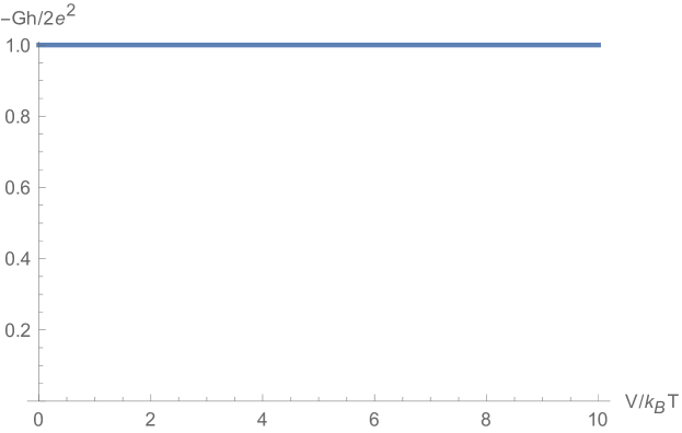
Figure 3: The conductance is given by $G=\frac{2e}{h}$.

The electrical conductance $G=\frac{2e^{2}}{h}$ is depicted in Fig. 3.

Next, we consider the thermoelectric effects . We attach a thermal reservoir at temperatures $T+\Delta T$ to the left and the reservoir at temperature $T$ to the right Mahan ; Butcher ; Bennakker . Considering the particle and anti-particle contributions, we find the following equation for the thermal conductivity:

$$\sum_{s=\pm}\langle J^{heat}_{+;s}(Q\rightarrow 0,\Omega\rightarrow 0)\rangle+\langle J^{heat}_{-;s}(Q\rightarrow 0,\Omega\rightarrow 0)\rangle=\hbar v^{2}\cdot$$

$$\int_{0}^{\Lambda}\frac{dq}{2\pi}\Big{[}(q-V)\Big{(}n_{F}(q-V)_{T+\Delta T}-n_{F}(q-V)_{T}\Big{)}+(q+V)\Big{(}(n_{F}(q+V)_{T+\Delta T}-n_{F}(q+V)_{T}\Big{)}\Big{]}$$

$$\approx 2\frac{K^{2}_{B}T}{h}(-\Delta T)\Big{[}\int_{\frac{-V}{K_{B}T}}^{\infty}x^{2}\partial_{x}n_{F}(x)dx+\int_{\frac{V}{K_{B}T}}^{\infty}x^{2}\partial_{x}n_{F}(x)dx\Big{]}$$

The finding is depicted in Figure $2$, $\kappa=\frac{2\pi^{2}K^{2}_{B}T}{3h}$.

The electric current generated by a thermal gradient is given by:

$$\sum_{s=\pm}\langle J^{el}_{+;s}(Q\rightarrow 0,\Omega\rightarrow 0)\rangle+\langle J^{el}_{-}(Q\rightarrow 0,\Omega\rightarrow 0)\rangle$$

$$=\int_{0}^{\Lambda}\frac{dq}{2\pi}ev|t|^{2}\Big{[}\Big{(}n_{F}(q-V)_{T+\Delta T}-n_{F}(q-V)_{T}-\Big{(}n_{F}(q+V)_{T+\Delta T}-n_{F}(q+V)_{T}\Big{)}\Big{]}$$

$$2\frac{eK_{B}}{h}(-\Delta T)\Big{[}\int_{-\frac{V}{K_{B}T}}^{\infty}x\partial_{x}n_{F}(x)dx+\int_{\frac{V}{K_{B}T}}^{\infty}x\partial_{x}n_{F}(x)dx\Big{]}$$

We observe that the thermoelectric conductance $L$ disappears, as shown in Figure $4$.

The temperature determins $N$, the number of excited transversal modes. As result the conductance $G$, the thermal conductance $kappa$, the thermoelectric conductance $L$ are replaced by:$G=N\frac{2e^{2}}{h}$, $\kappa=N\frac{2\pi^{2}}{3h}K^{2}_{B}T$ and $L=N\frac{2e}{h}K_{B}\cdot 0$.

IVb- The ballistic conductances for $|t|^{2}=1$

The thermal current for $|t(\epsilon)|^{2}=1$ for a finite size system of the size $L<1\mu$, and a temperature of $3K$. The energy in the lowest mode is $\epsilon_{0}=0.63\cdot 10^{-3}ev$ and the energies in the wire are $\epsilon_{n}=(n+\frac{1}{2})\epsilon_{0}$ . For a bandwidth of $0.1ev$ we will have $100$ modes. For a finite temperatures we have $N$ pair of channels.

The thermal conductance is given by :

$$I_{heat}=N\cdot\frac{v}{L}\sum_{n=1}^{n=160}$$

$$\Big{[}(\epsilon_{n}-V)\Big{(}n_{F}(\epsilon_{n}-V)_{T+\Delta T}-n_{F}(\epsilon_{n}-V)_{T}\Big{)}+(\epsilon_{n}+V)\Big{(}n_{F}(\epsilon_{n}+V)_{T+\Delta T}-n_{F}(\epsilon_{n}+V)_{T}\Big{)}\Big{]}$$

$$=N\cdot\frac{K_{B}Tv}{L}\sum_{n=1}^{n=200}$$

$$\Big{[}(\frac{\epsilon_{n}-V}{K_{B}T})\Big{(}n_{F}(\epsilon_{n}-V)_{T+\Delta T}-n_{F}(\epsilon_{n}-V)_{T}\Big{)}+(\frac{\epsilon_{n}+V}{K_{B}T})\Big{(}n_{F}(\epsilon_{n}+V)_{T+\Delta T}-n_{F}(\epsilon_{n}+V)_{T}\Big{)}\Big{]}$$

The heat current at $T=3K$ in Figure $5$ fluctuates as a function of the bias voltage $V$ measured in electron volts, $I_{heat}=NK_{B}T\frac{v}{L}[0.15-0.25]\frac{Joule}{sec}$.

The electrical conductance is shown in Figure $6$. The conductance oscillates as a function of the voltage bias $V$.

$$I_{el.}=N\cdot\frac{ev}{L}\cdot\sum_{n=1}^{n=160}\Big{[}\Big{(}n_{F}(\epsilon_{n}-V+eV_{G})_{T}-n_{F}(\epsilon_{n}-V)_{T}\Big{)}-\Big{(}n_{F}(\epsilon_{n}+V-eV_{G})_{T}-n_{F}(\epsilon_{n}+V)_{T}\Big{)}\Big{]}$$

The electrical current is $I_{el}=N\frac{ev}{L}[0.05-0.09]Ampere\approx N\cdot 10^{-7}[0.05-0.09]Ampere$.

The thermoelectric current is given by:

$$I_{el.}=N\cdot\frac{ev}{L}\cdot\sum_{n=1}^{n=160}\Big{[}\Big{(}n_{F}(\epsilon_{n}-V)_{T+\Delta T}-n_{F}(\epsilon_{n}-V)_{T}\Big{)}-\Big{(}n_{F}(\epsilon_{n}+V)_{T+\Delta T}-n_{F}(\epsilon_{n}+V)_{T}\Big{)}\Big{]}$$

The thermoelectric current in Figure $7$ shows strong oscillations as a function of the voltage bias $V$,$I_{el}=N\frac{ev}{L}[\pm 0.01]Ampere\approx N\cdot 10^{-7}[\pm 0.01]Ampere$ The results in Fiigure $7$ are in agreement with the experimental results Pepper in silicon where oscillations for the Seebeck coefficient have been reported as a function of the electronic density.

V-The conductances for the mesoscopic conditions

In order to have a finite scattering matrix element, we need to have backscattering. For this purpose, we use a model of a random magnetic field $(\sigma_{1}\otimes I)H_{x}(y)$ with the property : $\langle H_{x}(q)H_{x}(q^{\prime})\rangle=H_{sc}\delta[q+q^{\prime}]$. Such a model is obtained from a one dimensional configuration of paramagnetic impurities. Doping the Weyl semimetal surface with paramagnetic impurities in a narrow strip of width $d_{x}<D_{x}$ in the $x$ direction guarantees that the momentum scattering will be in the $y$ direction. Due to the spinor representation in Eq.(4) we find that the matrix elements $(\sigma_{x}\otimes I)$ are non-zero. For such a scattering potential we obtain:

$$\int_{-\infty}^{\infty}dy\psi^{\dagger}_{+,-;s}(y)(\eta_{+,-;s})^{\dagger}(\sigma_{x}\otimes I)\eta_{-,-;s}H_{x}(y))\psi_{-,-;s}(y)\neq 0$$

$$\int_{-\infty}^{\infty}dy\psi^{\dagger}_{-,-;s}(y)(\eta_{-,-;s})^{\dagger}(\sigma_{x}\otimes I))\eta_{+,-;s}H_{x}(y)\psi_{+,-;s}(y)\neq 0$$

$$\int_{-\infty}^{\infty}dy\psi^{\dagger}_{+,+;s}(y)(\eta_{+,+;s})^{\dagger}(\sigma_{x}\otimes I)\eta_{-,+;s}H_{x}(y))\psi_{-,+;s}(y)\neq 0$$

$$\int_{-\infty}^{\infty}dy\psi^{\dagger}_{-,+;s}(y)(\eta_{-,+;s})^{\dagger}(\sigma_{x}\otimes I))\eta_{+,+;s}H_{x}(y)\psi_{+,+;s}(y)\neq 0$$

Due to the spinor structure, $\eta_{\pm,+;s}$ and $\eta_{\pm,-;s}$ the scattering matrix elemets $(\sigma_{x}\otimes I)$ will occour between the pair with the same momentum $k_{x}$. The $\mathbf{S}$ matrix is identical for holes and particles and determin the transmission function $|t(\epsilon)|^{2}<1$. The transmission function is obtained from the $T$ matrix formula given in Eq. $5.40$ page $88$ Flensberg . For many channels, for the case $n_{xmax.}>N$ we have :

$$\Psi(x,y)=\sum_{s=\pm}\Big{[}\Big{(}e^{ik_{F}y}\psi_{+,-;s,}(y)\eta_{+,-;s}+e^{-ik_{F}y}\psi_{-,-;s,}(y)\Big{)}\eta_{-,-;s}+$$

$$\sum_{n_{x}=1}^{N}\Big{(}e^{ik_{F}y}\psi_{+,-;s,n_{x}}(x,y))\eta_{+,-;s}+e^{-ik_{F}y}\psi_{-,-;s,n_{x}}(x,y))\eta_{-,-;s}\Big{)}]$$

The scattering matrix with for a strip of paramagnetic impurities is given by the field $H_{x}(y)$.This field will generate backscattering matrix elements. Since the scattering potential is only a function of $y$, the backscattering will occur at the same momentum $k_{x}$.

In the case of $n_{x,max}<N$, we have the representation:

$$\Psi(x,y)=\sum_{s=\pm}\Big{[}\Big{(}e^{ik_{F}y}\psi_{+,-;s,}(y)\eta_{+,-;s}+e^{-ik_{F}y}\psi_{-,-;s,}(y)\Big{)}\eta_{-,-;s}+$$

$$\sum_{n_{x}=n_{x,max}}^{\infty}\Big{(}e^{ik_{F}y}\psi_{+,-;s,n_{x}}(x,y)\eta_{+,-;s}+e^{-ik_{F}y}\psi_{-,-;s,n_{x}}(x,y))\eta_{-,-;s}\Big{)}$$

$$+\sum_{s=\pm}\sum_{n_{x}=n_{x,max}}^{N}\Big{(}e^{ik_{F}y}\psi_{+,+;s,n_{x}}(x,y)\eta_{+,+;s}+e^{-ik_{F}y}\psi_{-,+;s,n_{x}}(x,y))\eta_{-,+;s}\Big{)}$$ (23)

In order to apply the Landau Buttiker theory we need to be under conditions where the elastic scattering length $l_{e}$ , the length of the system $L$ and the thermal length $L_{T}$ obey the relations $l_{e}\leq L\leq L_{T}$. $l_{e}$ is determined by the disorder. The use of a random field in the $x$ direction (or to have magnetic impurities) will generate backscattering. As a result for low temperatures we will be able to satisfy the condition $l_{e}\leq L\leq L_{T}$. We will consider a finite size system of the size $L<1\mu m$, and a temperature of $3K$. Due to the $(\sigma_{1}\otimes I)H_{x}(y)$ scattering field $\langle H_{x}(q)H_{x}(q^{\prime})\rangle=H_{sc}\delta[q+q^{\prime}]$ we will have localized states in one dimension . According to Weinberg the $\mathbf{S}$ matrix and the transmission matrix are given in Eqs.$3.2.7$ $3.2.8$. Eq.$3.5.3$ Weinberg contains an explicit form of the transmssion function from which we can obtain the transmission function in the Lorentz approximation at finite temperature:

$$|t(\epsilon)|^{2}\approx\sum_{n}\frac{(\frac{\Gamma}{2})^{2}}{(\epsilon-\epsilon_{n})^{2}+(\frac{\Gamma}{2})^{2}}$$

Using this approximation we compute the thermoelectric current.

$$I_{el.}=N\frac{e}{h}\int_{0}^{\infty}d\epsilon|t(\epsilon)|^{2}\Big{[}\Big{(}n_{F}(\epsilon-V)_{T+\Delta T}-n_{F}(\epsilon-V)_{T}\Big{)}-\Big{(}n_{F}(\epsilon+V)_{T+\Delta T}-n_{F}(\epsilon+V)_{T}\Big{)}\Big{]}$$

$$=N\frac{e}{h}K_{B}T\int_{0}^{\infty}dx|t(xK_{B}T)|^{2}\Big{[}\Big{[}\Big{(}n_{F}(x-\frac{V}{K_{B}(T+\Delta T)}\Big{)}-\Big{(}n_{F}(x-\frac{V}{K_{B}T}\Big{)}\Big{]}$$

$$-\Big{[}\Big{(}n_{F}(x+\frac{V}{K_{B}(T+\Delta T)}\Big{)}-n_{F}\Big{(}x+\frac{V}{K_{B}T}\Big{)}\Big{]}\Big{]}$$

This result is presented in Figure 9. Comparing the thermoelectric current in Figure $7$ with Figure $9$, we observe that the reduction in the transmission function decreases the thermoelectric current. Figure $9$ also show that at small voltages bias the thermoelectric current is enhanced.

VI- Proposed experimental set up for testing thermoelectricity

We will chose a Weyl semimetal material with the surface at $z=0$ and width few millimeters in the $z$ direction.To be in the mesoscopic regime the temperature should be below $5k$ , the length in the $y$ direction $\approx 1\mu m$ and the width in the $x$ direction below $0.1\mu m$. On the left side of the sample we apply a heating device which will create a temperature $T+\Delta T$ The right side of the sample is held at temperature $T$. A random magnetic field or paramagnetic impurities on the surface are requiered in order to observe backscattering .The field is $y$ dependent. Backscattering will occur only when the right and left channel have the same momentum $k_{x}$. As result, we will observe a thermoelectric voltage between the left and right side of the sample. The sign of the voltage will depend on the value of the voltage $V$ bias. In the z direction we have a crystal of milimeter length. Our computation predicts that for perfect transmission $|t|^{2}=1$ (absence of backscattering) the thermoelectric cuurent is significantly higher than the thermoelectric current obtained when backscattering is allowed. This symmetry afects the value of the thermoelectric current and can be used as a detection signature. At low temperature we have only one channel , $N=1$. With the increases of the temperature the conductances will scale with the factor $N$, but the ratio between the conductances with and without backscattering will be $N$ independent.

VII-Conclusion

Quantum effects are predicted for thermoelectricity. The computation is performed for surface zero modes which are protected against backscattering. The effect of magnetic impurities allows to probe the thermal effect as function of the scattering length $l_{e}$ and confirm the oscillation of the thermoelectric conductance as a function of the voltage bias. An experimental set up was proposed to test our theory.

Figure 1: The one dimensional propagating channels as a function of the momentum $k_{x}=\pm\frac{2\pi}{D_{x}}(n_{x}+\frac{1}{2})$. The figure shows a finite number of channels. We observe that for each momentum $k_{x}$ we have two conducting channels.

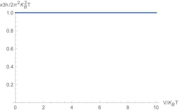
Figure 2: The thermal conductance is $\kappa=\frac{\pi^{2}K^{2}_{B}T}{3h}I[\frac{V}{K_{B}T}]$ where $I[\frac{V}{K_{B}T}]\approx 1$, $|t|^{2}=1$

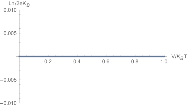
Figure 4: The thermoelectric conductance $L=\frac{2e}{h}K_{B}$ for the transmission $|t(\epsilon)|^{2}=1$

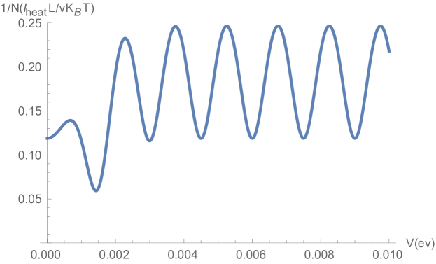
Figure 5: The thermal heat current plot is given for a temperature $T\approx 3$ (see figure $5$ ) as a function of the voltage bias $V=\hbar v(k_{0}-k_{F})$ ,the velocity was $10^{5}\frac{m}{sec}$ and the temperature difference was $0.1K$ .This figure includes ncludes particle and hole contributions . The heat current fluctuates as a function of the bias voltage $V$ measured in electron volt, $I_{heat}=NK_{B}T\frac{v}{L}[0.15-0.25]\frac{Joule}{sec}$

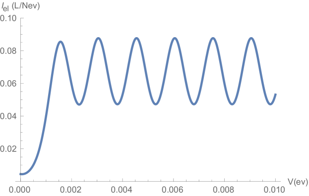
Figure 6: The electrical conductance at $3k$ for $eV_{G}=0.0001ev$. $I_{el.}=N\cdot\frac{ev}{L}[0.04-0.08]Ampere.$

Figure 7: The Thermoelectric current for the transmission $|t(\epsilon)|^{2}=1$. $I_{el.}=N\cdot\frac{ev}{L}...\pm 0.02Ampere$

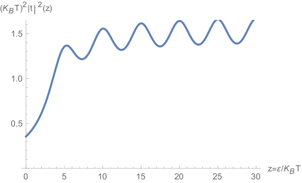
Figure 8: The transmission function $|t(\epsilon)|^{2}\approx\sum_{n}\frac{(\frac{\Gamma}{2})^{2}}{(\epsilon-\epsilon_{n})^{2}+(\frac{\Gamma}{2})^{2}}$ .We show results for the case that $\epsilon_{0}\approx\Gamma$.

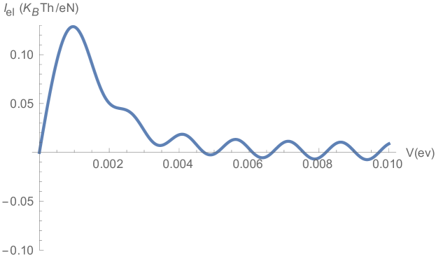
Figure 9: The thermoelectric current for the mesoscopic case is $I_{el.}=N\frac{eK_{B}T}{h}\pm 0.015....Ampere$ , $\delta T=0.1K$ at $T=3K$.

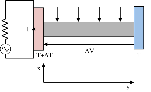
Figure 10: The proposed experiment.The effect of the paramagnetic impurities is showing by the arrow in the $x$ direction in the figure. We mention that the effect of the random paramagnetic impurities can be achived by applyng a magnetic field of $1milimeter$ wavelength.The left side of the sample is connected to a current$I$ to create a elevated temperature $T+\Delta T$ with trespect the right side. A voltage $\Delta V$ is induced by the temperature difference

References

• (1) H.J.Goldsmith ”Thermoelectric Refrigeration(Plenum,New York 1964) Introduction to thermoelectricity (Springer -Verlag,Berlin,Heidelberg,2010)
• (2) Kamran Behnia ”Fundamentals of Thermoelectricity”Oxford University Press 2015.
• (3) Vijay Narayan ,Michael Pepper, David A.Ritchie, Cond-Matt 1605.073741v1
• (4) Mitali Banerjee , Moty Heilblum ,Vladimir Umansky ,Dima Feldman,Yuval Oreg,and Ady Stern Cond-Matt.1710.00492
• (5) D.Schmeltzer ”The S matrix for surface boundary states :An application to photoemission for Weyl semimetals” https:// doi.org/1016/j. aop. 2018 .04.018, Annals of Physics
• (6) E. Witten, arXiv :cond-mat/1510.07698 and Reviews of Modern Physics 88,035001 (2016) see Eq.(3.12) on page 035001 -23.
• (7) Butcher J.Phys.Cond. Martter 2 4869 (1990)
• (8) H.Nielsen and M.Ninomiya,Phys.Lett. B 130, 389 (1983).
• (9) G.D.Mahan, and J.O. Sofo Proc. Nat.Acad. Sci. 93,7468 (1996)
• (10) Alexander Altland and Dmitry Bagreys Phys.Rev.Lett 114,257201 (2015)
• (11) Su-Yang Xu, Ilya Belopolski,Nasser Alidoust, Madhab Neupaine, Guang Bian, Chenglong Zhang, Raman Sankar, Guoqing Chang, Zhujun Yuan, Chi-Cheng Lee, Shin-Ming Huang, Hao Zheng, Jie Ma, Daniel S.Sanchez, BaoKai Wang, Arun Bansil, Fangcheng Chou, Pavel P.Shibayev, Hsin Lin, Shuang Jia, M.Zahid Hasan Science, vol. 349 ISSUE 6248 (2015)
• (12) H.van Houten, L.W. Molenkamp,C.W. Beenakker and C.T. Foxon Semiconductor Sience and Technology 7, B215-B221 (1992)
• (13) R. Shankar ”Quantum Field Theory and Condensed Matter”An Introduction Cambridge University Press (2017)
• (14) M Buttiker Phys.Rev.Lett.57,1761(1996)
• (15) Henrick Bruus and Karsten Flensberg ”Many-Body Quantum Theory in Condensed Matter Physics” An Introduction. Oxford University Press 2016,pages 102-111.
• (16) Steven Weinberg ”The Quantum Theory of Fields” Cambridge Press 1995.
Refer to caption