DMCNN: Dual-Domain Multi-scale Convolutional neural Network for Compression Artifacts Removal

Abstract

JPEG is one of the most commonly used standards among lossy image compression methods. However, JPEG compression inevitably introduces various kinds of artifacts, especially at high compression rates, which could greatly affect the Quality of Experience (QoE). Recently, convolutional neural network (CNN) based methods have shown excellent performance for removing the JPEG artifacts. Lots of efforts have been made to deepen the CNNs and extract deeper features, while relatively few works pay attention to the receptive field of the network. In this paper, we illustrate that the quality of output images can be significantly improved by enlarging the receptive fields in many cases. One step further, we propose a Dual-domain Multi-scale CNN (DMCNN) to take full advantage of redundancies on both the pixel and DCT domains. Experiments show that DMCNN sets a new state-of-the-art for the task of JPEG artifact removal.

Index Terms—  Compression Artifacts Removal, Image Restoration, JPEG, Convolutional Neural Network

1 Introduction

Nowadays, lossy image compression methods (e.g. JPEG, HEVC-MSP and WebP) have been used extensively for image storage and transmission. These methods typically shrink parts of image information by quantization and approximation, so that higher compression rates can be reached. These methods can usually reduce the bit-rate greatly but still maintain satisfactory visual quality by taking advantage of the limitation of the human visual system. But as the compression rate increases, these methods tend to introduce undesirable artifacts such as blocking, ringing, and banding. These artifacts severely degrade the user experience.

In this paper, we examine the degradation of JPEG-compressed images. Typically, a JPEG compressor converts an image of RGB color space into the YCbCr color space. The chroma channels (namely Cb and Cr) are downsampled by the factor of 2. Then, the image is partitioned into $8\times 8$ blocks and the block-wise 2D Discrete Cosine Transform (DCT) is performed. After DCT, the top left items in each $8\times 8$ block are low-frequency components, representing the overall features such as the average luminance. The bottom right items are high-frequency components, representing local features such as textures and details. Next, quantization is applied on each of 64 DCT coefficients. As human eyes are not so good at distinguishing high frequency brightness variation, quantization intervals are typically much larger on high-frequency components than low-frequency ones. Noting that the quantization step is the culprit for various kinds of artifacts such as the blocking artifacts within the boundaries of each $8\times 8$ DCT block, the ringing artifacts around sharp edges, and the noticable banding effects over the image. As a matter of fact, these kinds of artifacts can be commonly seen on other transform-based methods.

Many methods have been proposed to improve the quality of JPEG-compressed images. Traditional filter-based methods [1, 2] pay attention to general images denoising. Others apply the sparse coding (SC) to restore the compressed images [3, 4]. These methods generally produce sharper images given a compressed input, but they are usually too slow and their results are often accompanied with additional artifacts.

With the rapid development of deep neural networks, multiple CNN-based methods have been used in low-level image processing, including denoising [5, 6], super-resolution [7, 8, 9], video compression [10, 11], rain removal [12, 13, 14]. Specifically for compression artifacts removal, Dong et al. [15] first introduce a CNN-based method and the proposed ARCNN set a good practice for the following low-level CNN-based methods including DnCNN [5], CAS-CNN [16], and MemNet [17]. However, these methods usually work on pixel domain only and do not incorporate much JPEG prior knowledge. More recently, a dual-domain CNN-based model DDCN is proposed in [18]. The model sucessfully combines DCT-domain prior and the power of the CNN, thus achieves impressive performance.

However, a common weakness of all these CNN-based methods is that the receptive fields of their models are too small, and these models are usually trained on mini image patches (e.g. $35\times 35$ for ARCNN, $49\times 49$ for DnCNN, $55\times 55$ for DDCN), so that only a small range of information (i.e. neighbor pixels) are taken into consideration when performing the restoration. Noting that local information is sometimes not enough to remove all the artifacts, especially the banding effects, which can appear at a large scale on the image. As shown in Fig. 1, due to the quantization step of JPEG, the sky in the image is split into multiple bandings, and ARCNN fails to recover the bandings because of small receptive fields.

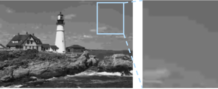
Fig. 1: The banding effects can still be clearly seen after the process of ARCNN (QF=10).

To eliminate the banding effects, three efforts have been made to enlarge the receptive fields and enable our model with the ability of extracting global features: (1) Auto-encoder style architecture; (2) Dilated convolutions; (3) Multi-scale loss. Moreover, as validated by DDCN, redundancies in the DCT domain can be effectively utilized. We also adopt a DCT domain branch to enhance the performance of the proposed model.

Our major contribution is to propose an end-to-end CNN with large receptive fields to exploit dual-domain multi-scale features. In order to train the proposed DMCNN more effectively, a modified version of residual learning as well as other training techniques have been utilized. The evaluations on the BSDS500 and the LIVE1 dataset have shown that our work is the current state-of-the-art among all CNN-based JPEG artifact removal networks.

2 Dual-Domain Multi-scale Convolutional Neural Network (DMCNN)

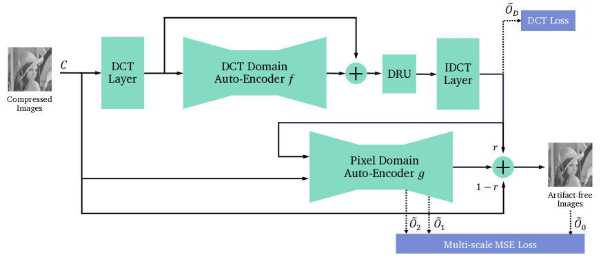
Fig. 2: The architecture of Dual-domain Multi-scale Convolutional Network (DMCNN).

The architecture of our proposed DMCNN is in Fig. 2. The model is mainly composed of two similar auto-encoder style networks working on pixel and DCT domains, respectively. The input image is processed by DCT branch first, then passed into the pixel domain branch. The final restoration result is the weighted sum of the input, the DCT branch estimation and the pixel branch estimation.

2.1 Auto-Encoder

The auto-encoder is an efficient way to learn a representation for given data, and typically used for the purpose of dimensionality reduction. An auto-encoder consists of two parts, the encoder $E$ and the decoder $D$, so that:

$$E :\mathcal{X}\rightarrow\mathcal{F},$$ (1)

$$D :\mathcal{F}\rightarrow\mathcal{X},$$

$$E,D= {\underset{E,D}{\operatorname{arg\,min}}}\,\|x-(D\circ E)x\|^{2},$$

where $\mathcal{X}$ denotes the set of the to-be-compressed data, $\mathcal{F}$ denotes the feature space and $\circ$ is the composition operator. Typically, an auto-encoder is trained with identical image pairs $(x,x)\in\mathcal{X}\times\mathcal{X}$, so that $E$ could learn to extract the best representation of the data in $\mathcal{F}$.

We adopt an auto-encoder style network here as a generative model. Given a compressed image, the encoder $E$ is expected to extract artifact-free features robustly, and then the image is restored from these clean features by decoder $D$.

In order to learn both local and global features, shortcuts are linked between symmetric layers. Also, residual learning strategy is employed. To stress the information learnt form the DCT domain, we add a shortcut with parameter $r$ from the DCT-branch into the final result. Given an input image $C$, the intermediate estimation of the DCT branch $\tilde{O}_{D}$ and the final output $\tilde{O}_{0}$ can be fomulated as:

$$\tilde{O}_{D} =\mathcal{D}^{-1}([f(\mathcal{D}(C))]_{\text{DRU}}),$$ (2)

$$\tilde{O}_{0} =g(C,\tilde{O}_{D})+r\tilde{O}_{D}+(1-r)C,$$

where $\mathcal{D}$ and $\mathcal{D}^{-1}$ stand for the process of $8\times 8$ block-wise DCT and inverse DCT (IDCT) respectively. $f(\cdot)$ and $g(\cdot)$ denote the processes of the DCT domain auto-encoder and the pixel domain auto-encoder, respectively. $[\cdot]_{\text{DRU}}$ denotes the DCT Rectify Unit stated later, and $r$ is a learnable parameter of the residual addition module.

2.2 Dilated Convolution

The dilated convolution is a kind of convolution with pre-defined gaps, it is first named in [19]. Consider an input image $I$ as a discrete function $I:\mathbb{Z}^{2}\rightarrow\mathbb{R}$ and a convolution kernel $k$ shaped $(2r+1)\times(2r+1)$ as a discrete function $k:\Omega_{r}\rightarrow\mathbb{R}$, where $\Omega_{r}=[-r,r]^{2}\cap\mathbb{Z}^{2}$. The discrete convolution operator $*_{d}$ with dilation factor $d$ can be defined as:

$$(I*_{d}k)(\mathbf{p})=\sum_{\mathbf{s}+d\mathbf{t}=\mathbf{p}}{I(\mathbf{s})k(\mathbf{t})},$$ (3)

where $\mathbf{p},\mathbf{s},\mathbf{t}\in\mathbb{Z}^{2}$ are 2D indices.

Unlike normal convolutions, the receptive field of $n$ combined dilated convolutions can reach $(2^{n-1}-1)\times(2^{n-1}-1)$ when dilation factors are set to $1,2,4,...,2^{n-1}$, respectively. The dilated convolution has been widely used in other vision tasks [20, 21] and shown considerable gain, but to the best of our knowledge, has not been used in the task of artifacts removal. In our model, the dilated convolutional layers with dilation factors 2, 4, 8 are used in the middle of the auto-encoder, which aim to enlarge the receptive field further.

With the combination of auto-encoder style architecture and dilated convolutions, the receptive field of our proposed DMCNN reaches $145\times 145$, which is about 58 times larger than the ARCNN ($19\times 19$), and 13 times larger than the DnCNN and the DDCN ($41\times 41$).

2.3 DCT Rectify Unit (DRU)

As stated earlier in the introduction, the main cause of the JPEG compression artifacts is the step of quantization. The quantization step in each of the $8\times 8$ compression blocks can be formulated as follows:

$$C^{\text{DCT}}(\mathbf{p})=\text{round}(O^{\text{DCT}}(\mathbf{p})/Q(\mathbf{p}))*Q(\mathbf{p}),$$ (4)

where $C^{\text{DCT}}$ is the quantized DCT block, $O^{\text{DCT}}$ is the original DCT block, $Q$ is the quantization table, and $\mathbf{p}\in\mathbb{Z}^{2}$ is a 2D index. $/$ here denotes the element-wise division.

From $(4)$, it can be easily seen that the estimated $\tilde{O}^{\text{DCT}}$ should meet the requirement:

$$C^{\text{DCT}}-Q/2\leq\tilde{O}^{\text{DCT}}\leq C^{\text{DCT}}+Q/2.$$ (5)

So like [18] we employ a DCT Rectify Unit (DRU) to constraint the value of DCT block elements, where values out of the range will be cropped. A slight difference is that we drop the leaky slope $\alpha$ in their proposed unit, as no gain can be observed with it. Our DRU can be formulated as:

$$[X]_{\text{DRU}}(\mathbf{p})=\begin{cases}C^{\text{DCT}}(\mathbf{p})-Q(\mathbf{p})/2,&X(\mathbf{p})<C^{\text{DCT}}(\mathbf{p})-Q(\mathbf{p})/2,\\ C^{\text{DCT}}(\mathbf{p})+Q(\mathbf{p})/2,&X(\mathbf{p})>C^{\text{DCT}}(\mathbf{p})+Q(\mathbf{p})/2,\\ X(\mathbf{p}),&\text{otherwise}.\end{cases}$$ (6)

2.4 Multi-scale DCT-Embedded Loss

As is pointed out by previous works [22] [15], “deeper is not better” in certain low-level tasks. The reason is that deeper neural networks are usually harder to train due to the gradient vanishing. We try to address this problem by redesigning the loss function of the model.

A multi-scale loss is adopted to extract features at different scales. More specifically, features are extracted from different deconvolutional layers of the pixel domain decoder, and scaled images are expected to be reconstructed from these features. By adopting the multi-scale loss, we explicitly guide our network to learn features at different scales.

We also add a DCT loss to train the DCT branch more effectively. Finally, our loss function can be stated as:

$$\mathcal{L}({\{\tilde{O}\}}_{i=0}^{2},\tilde{O}_{D},\{O\}_{i=0}^{2})$$ (7)

$$=\mathcal{L}_{\text{MMSE}}(\{\tilde{O}\}_{i=0}^{2},\{O\}_{i=0}^{2})+\lambda\mathcal{L}_{\text{DCT}}(\tilde{O}_{D},O_{0})$$

$$=\sum_{i=0}^{2}{\theta^{i}\text{MSE}(\tilde{O}_{i},O_{i})}+\lambda\text{MSE}(\tilde{O}_{D},O_{0}),$$

where ${\{\tilde{O}\}}_{i=0}^{2}$ are estimations from pixel domain auto-encoder at different scales, $\{O\}_{i=0}^{2}$ are original images at different scales, and $\tilde{O}_{D}$ is the intermeidate estimation of the DCT branch. Hyper-parameters $\lambda$ and $\theta$ are used to adjust the weights of each loss, they should typically be in the range of $[0,1]$. MSE($\cdot$,$\cdot$) denotes the mean squared error loss.

3 Experiments

3.1 Implement Details

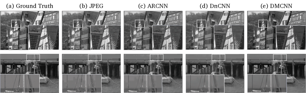
Fig. 3: Visual comparisons between different algorithms with QF=10. Zooming-in the figure will provide a better look at the restoration quality.

Datasets.  In all experiments, we employ the ImageNet [23] for training. The LIVE1 dataset and the testing set of BSDS500 are used for evaluation. All training and evaluation processes are done on gray-scale images (the Y channel of YCbCr space). The PIL module of python is applied to generate JPEG-compressed images. The module produces numerically identical images as the commonly used MATLAB JPEG encoder after setting the quantization tables manually.

Parameter Settings.  The hyper-parameters $\lambda$ and $\theta$ are set to $0.9$ and $0.618$, respectively. The parameter $r$ of final residual links is initialized to $0.5$. The DCT and IDCT layers are fixed and initialized with the corresponding DCT matrix coefficients. Leaky slopes are initialized to $0.1$ for PReLUs. The depth of the pixel and DCT domain auto-encoders are 15 and 9, respectively.

Training Details.  Adam optimizer with initial learning rate 0.001 is used for training. The learning rate is scaled down by the factor of 3 when the validation loss stops decreasing. The batch size is set to 80. Training pairs are dynamically generated from the training set. The sizes of training patches are not fixed. As an easy-to-hard transfer, we first train our model on pairs generated with quality factor (QF) of 20 and patch size of $56\times 56$. Then we gradually increase the patch size till $224\times 224$. After full convergence, the model dedicated to QF10 is trained based on the previous QF20 model.

3.2 Objective Comparisons

To have overall comparisons, we calculate the mean PSNR, SSIM [24], and PSNR-B [25] on the two datasets. We compare to recent state-of-the-arts including pixel domain methods – ARCNN and CAS-CNN, dual domain method – DDCN and general frameworks – TNRD [26] and DnCNN[5].

The quantitative results are shown in Table.1 and Table.2. Generally, our proposed model DMCNN outperforms all the other methods on all evaluated datasets, QFs and metrics. Specifically, our model far surpasses all pixel domain methods and general frameworks. Also, considerable gains can be observed compared to the dual domain method DDCN.

Table 1: The quantitative results on LIVE1.

QF	Method	PSNR(dB)	SSIM	PSNR-B(dB)
10	JPEG	27.77	0.791	25.33
	ARCNN [15]	29.13	0.823	28.74
	TNRD [26]	29.24	0.825	28.90
	DnCNN-3 [5]	29.27	0.825	28.98
	CAS-CNN [16]	29.44	0.833	29.19
	DMCNN	29.73	0.842	29.55
20	JPEG	30.07	0.868	27.57
	ARCNN [15]	31.40	0.890	30.69
	TNRD [26]	31.52	0.892	30.88
	DnCNN-3 [5]	31.62	0.894	30.89
	CAS-CNN [16]	31.70	0.895	30.88
	DMCNN	32.09	0.905	31.32

Table 2: The quantitative results on BSDS500 testing set.

QF	Method	PSNR(dB)	SSIM	PSNR-B(dB)
10	JPEG	27.80	0.788	25.10
	ARCNN [15]	29.10	0.820	28.73
	TNRD [26]	29.16	0.823	28.81
	DnCNN-3 [5]	29.17	0.823	28.91
	DDCN [18]	29.59	0.838	29.18
	DMCNN	29.67	0.840	29.33
20	JPEG	30.05	0.867	27.22
	ARCNN [15]	31.28	0.885	30.55
	TNRD [26]	31.41	0.889	30.83
	DnCNN-3 [5]	31.50	0.891	30.85
	DDCN [18]	31.88	0.900	31.10
	DMCNN	31.98	0.904	31.29

3.3 Subjective Comparisons

For subjective comparisons, some restored images of different approches on the LIVE1 dataset have been presented. As can be seen in Fig. 3, the results of DMCNN are more visually pleasing. Due to the large receptive fields, our model is able to handle quantization banding effects as well as recover lost details using regional patterns. More experiment results are available on our project page .

4 Conclusions

In this paper, we introduce a novel network based on dual-domain auto-encoders, named DMCNN. By applying dilated convolutional layers and multi-scale loss, our model is able to extract global information and eliminate JPEG compression artifacts effectively.

References

- [1] Alessandro Foi, Vladimir Katkovnik, and Karen Egiazarian, “Pointwise shape-adaptive dct for high-quality denoising and deblocking of grayscale and color images,” IEEE Transactions on Image Processing, vol. 16, no. 5, pp. 1395–1411, 2007.
- [2] Kostadin Dabov, Alessandro Foi, Vladimir Katkovnik, and Karen Egiazarian, “Image denoising by sparse 3-d transform-domain collaborative filtering,” IEEE Transactions on Image Processing, vol. 16, no. 8, pp. 2080–2095, 2007.
- [3] Huibin Chang, Michael K Ng, and Tieyong Zeng, “Reducing artifacts in jpeg decompression via a learned dictionary,” IEEE Transactions on Signal Processing, vol. 62, no. 3, pp. 718–728, 2014.
- [4] Xianming Liu, Xiaolin Wu, Jiantao Zhou, and Debin Zhao, “Data-driven sparsity-based restoration of jpeg-compressed images in dual transform-pixel domain.,” in Proceedings of the IEEE International Conference on Computer Vision and Pattern Recognition, 2015, vol. 1, p. 5.
- [5] Kai Zhang, Wangmeng Zuo, Yunjin Chen, Deyu Meng, and Lei Zhang, “Beyond a Gaussian denoiser: Residual learning of deep CNN for image denoising,” IEEE Transactions on Image Processing, vol. 26, no. 7, pp. 3142–3155, 2017.
- [6] Xiaoshuai Zhang, Yiping Lu, Jiaying Liu, and Bin Dong, “Dynamically unfolding recurrent restorer: A moving endpoint control method for image restoration,” arXiv preprint arXiv:1805.07709, 2018.
- [7] Chao Dong, Chen Change Loy, Kaiming He, and Xiaoou Tang, “Image super-resolution using deep convolutional networks,” IEEE Transactions on Pattern Analysis and Machine Intelligence, vol. 38, no. 2, pp. 295–307, Feb 2016.
- [8] Wenhan Yang, Sifeng Xia, Jiaying Liu, and Zongming Guo, “Reference guided deep super-resolution via manifold localized external compensation,” IEEE Transactions on Circuits and Systems for Video Technology, pp. 1–1, 2018.
- [9] Wenhan Yang, Jiashi Feng, Guosen Xie, Jiaying Liu, Zongming Guo, and Shuicheng Yan, “Video super-resolution based on spatial-temporal recurrent residual networks,” Computer Vision and Image Understanding, vol. 168, pp. 79 – 92, 2018.
- [10] Yueyu Hu, Wenhan Yang, Sifeng Xia, Wen-Huang Cheng, and Jiaying Liu, “Enhanced intra prediction with recurrent neural network in video coding,” in Proceedings of Data Compression Conference, March 2018.
- [11] Sifeng Xia, Wenhan Yang, Yueyu Hu, Siwei Ma, and Jiaying Liu, “A group variational transformation neural network for fractional interpolation of video coding,” in Proceedings of Data Compression Conference, March 2018.
- [12] Xueyang Fu, Jiabin Huang, Delu Zeng, Yue Huang, Xinghao Ding, and John Paisley, “Removing rain from single images via a deep detail network,” in Proceedings of the IEEE International Conference on Computer Vision and Pattern Recognition, July 2017.
- [13] Rui Qian, Robby T. Tan, Wenhan Yang, Jiajun Su, and Jiaying Liu, “Attentive generative adversarial network for raindrop removal from a single image,” in Proceedings of the IEEE International Conference on Computer Vision and Pattern Recognition, June 2018.
- [14] Jiaying Liu, Wenhan Yang, Shuai Yang, and Zongming Guo, “Erase or fill? deep joint recurrent rain removal and reconstruction in videos,” in Proceedings of the IEEE International Conference on Computer Vision and Pattern Recognition, June 2018.
- [15] Chao Dong, Yubin Deng, Chen Change Loy, and Xiaoou Tang, “Compression artifacts reduction by a deep convolutional network,” in Proceedings of the IEEE International Conference on Computer Vision, 2015, pp. 576–584.
- [16] Lukas Cavigelli, Pascal Hager, and Luca Benini, “Cas-cnn: A deep convolutional neural network for image compression artifact suppression,” in Proceedings of the International Joint Conference on Neural Networks (IJCNN). IEEE, 2017, pp. 752–759.
- [17] Ying Tai, Jian Yang, Xiaoming Liu, and Chunyan Xu, “Memnet: A persistent memory network for image restoration,” in Proceedings of the IEEE Conference on Computer Vision and Pattern Recognition, 2017, pp. 4539–4547.
- [18] Jun Guo and Hongyang Chao, “Building dual-domain representations for compression artifacts reduction,” in Proceedings of the European Conference on Computer Vision. Springer, 2016, pp. 628–644.
- [19] Fisher Yu and Vladlen Koltun, “Multi-scale context aggregation by dilated convolutions,” in Proceedings of the International Conference on Learning Representations, 2016.
- [20] Liang-Chieh Chen, George Papandreou, Iasonas Kokkinos, Kevin Murphy, and Alan L Yuille, “Deeplab: Semantic image segmentation with deep convolutional nets, atrous convolution, and fully connected crfs,” arXiv preprint arXiv:1606.00915, 2016.
- [21] Qiang Wang, Huijie Fan, Yang Cong, and Yandong Tang, “Large receptive field convolutional neural network for image super-resolution,” in Proceedings of 2017 IEEE International Conference on Image Processing. IEEE, 2017, pp. 958–962.
- [22] Chao Dong, Chen Change Loy, Kaiming He, and Xiaoou Tang, “Learning a deep convolutional network for image super-resolution,” in Proceedings of the European Conference on Computer Vision. Springer, 2014, pp. 184–199.
- [23] Olga Russakovsky, Jia Deng, Hao Su, Jonathan Krause, Sanjeev Satheesh, Sean Ma, Zhiheng Huang, Andrej Karpathy, Aditya Khosla, Michael Bernstein, Alexander C. Berg, and Li Fei-Fei, “ImageNet Large Scale Visual Recognition Challenge,” International Journal of Computer Vision (IJCV), vol. 115, no. 3, pp. 211–252, 2015.
- [24] Zhou Wang, Alan C Bovik, Hamid R Sheikh, and Eero P Simoncelli, “Image quality assessment: from error visibility to structural similarity,” IEEE Transactions on Image Processing, vol. 13, no. 4, pp. 600–612, 2004.
- [25] Changhoon Yim and Alan Conrad Bovik, “Quality assessment of deblocked images,” IEEE Transactions on Image Processing, vol. 20, no. 1, pp. 88–98, 2011.
- [26] Yunjin Chen and Thomas Pock, “Trainable nonlinear reaction diffusion: A flexible framework for fast and effective image restoration,” IEEE Transactions on Pattern Analysis and Machine Intelligence, vol. 39, no. 6, pp. 1256–1272, 2017.