ExoMol line lists XXVIII: The rovibronic spectrum of AlH

Abstract

A new line list for AlH is produced. The WYLLoT line list spans two electronic states $X\,{}^{1}\Sigma^{+}$ and $A\,{}^{1}\Pi$. A diabatic model is used to model the shallow potential energy curve of the $A\,{}^{1}\Pi$ state, which has a strong pre-dissociative character with only two bound vibrational states. Both potential energy curves are empirical and were obtained by fitting to experimentally derived energies of the $X\,{}^{1}\Sigma^{+}$ and $A\,{}^{1}\Pi$ electronic states using the diatomic nuclear motion codes Level and Duo. High temperature line lists plus partition functions and lifetimes for three isotopologues ²⁷AlH, ²⁷AlD and ²⁶AlH were generated using ab initio dipole moments. The line lists cover both the $X$–$X$ and $A$–$X$ systems and are made available in electronic form at the CDS and ExoMol databases.

1 Introduction

Aluminium is one of the commoner interstellar metallic elements, with a cosmic abundance of Al/H = $3\times 10^{-6}$ but AlH has only been rather sparingly observed. AlH was detected in the photospheres of $\chi$ Cygni, a Mira-variable S-star, by Herbig (1956) and much more recently around Mira-variable o Ceti by Kaminski et al. (2016). AlH was also detected in sunspots through lines in its $A\,{}^{1}\Pi$ – $X\,{}^{1}\Sigma^{+}$ electronic band, which lies in the blue region of the visible (Wallace et al., 2000); this spectrum was recently analysed for its rotational temperature by Karthikeyan et al. (2010).

AlH is difficult to detect in the interstellar medium because of its small reduced mass, which causes its rotational transitions to occur in the submillimetre region. This spectral region is typically filtered by terrestrial atmospheric effects, therefore making it difficult to detect from ground-based observations. So far searches for interstellar AlH have proved negative with, for example, only an upper limit set for the molecule rich IRC+10216 (Cernicharo et al., 2010) using the Herschel Space Observatory. Halfen & Ziurys (2010, 2014, 2016) have undertaken systematic improvement of the AlH submillimetre frequencies, including hyperfine splittings, to aid future detections. The work of Halfen & Ziurys is directly complementary to the work presented here which is aimed at providing ro-vibrational and rovibronic spectroscopic data. Other laboratory studies of AlH spectra, both experimental and theoretical, are discussed below.

Molecular spectra are useful for providing isotopic abundances. Aluminium has only one stable isotope, ²⁷Al, but ²⁶Al has a long half-life, in excess of 700 000 years. The mass fraction ratio of interstellar ²⁷Al to ²⁶Al can therefore provide important information on the formation of Al isotopes (Mahoney et al., 1984; Diehl et al., 2003; Lugaro et al., 2012); these could be probed using the spectrum of AlH. The AlH molecule is also thought to be an important constituent of the atmospheres of so-called Lava-planets (Tennyson & Yurchenko, 2017).

The $A$–$X$ band has also been considered as a possible means of producing ultra-cold AlH using laser cooling (Wells & Lane, 2011). Lifetimes of the $A\,{}^{1}\Pi$ state were measured by Baltayan & Nedelec (1979), while Tao et al. (2003) considered lifetimes for the triplet system $b$–$a$.

Bauschlicher & Langhoff (1988) used a full configuration interaction (FCI) ab initio method to produce ab initio potential energy and dipole moment curves of AlH, where they also estimated the dissociation energies of the $X\,{}^{1}\Sigma^{+}$ and $A\,{}^{1}\Pi$ states and lifetimes of the two bound vibrational sates of $A\,{}^{1}\Pi$. The heat of formation of AlH was estimated by Cobos (2002) using DFT methods. Cave et al. (1994) presented ab initio estimates for the dipole moments and transition dipole moments of AlH using a quasi-degenerate variational perturbation theory and averaged coupled-pair functional theory.

The ExoMol project (Tennyson & Yurchenko, 2012) aims to provide line lists of spectroscopic transitions for key molecular species which are likely to be important in the atmospheres of extrasolar planets and cool stars. Rajpurohit et al. (2013) analysed BT-Settl synthetic spectra (Allard, 2014) for M-dwarf stars and suggested that the CaOH band at 5570 Å, and AlH and NaH hydrides in the blue part of the spectra constituted the main species still missing in the models. An ExoMol line list for NaH was subsequently computed by Rivlin et al. (2015); here we construct the corresponding line lists for isotopologues ²⁷AlH, ²⁷AlD and ²⁶AlH of aluminium hydride.

We previously provided line lists for isotopologues of AlO (Patrascu et al., 2015); this work follows closely on the methodology developed for treating this open shell system (Patrascu et al., 2014). Here we consider transitions within the $X\,{}^{1}\Sigma^{+}$–$X\,{}^{1}\Sigma^{+}$ and electronic $A\,{}^{1}\Pi$ – $X\,{}^{1}\Sigma^{+}$ bands. The $A\,{}^{1}\Pi$ potential energy curve (PEC) is very shallow with a strong pre-dissociative character and can accommodate only two vibrational states (Holst & Hulthén, 1934) with a small barrier before the dissociation. Here we apply the Duo diatomic code (Yurchenko et al., 2016) to solve the nuclear motion problem for the $X\,{}^{1}\Sigma^{+}$ and $A\,{}^{1}\Pi$ coupled electronic states of AlH and to generate a line list for the $X$–$X$ and $A$–$X$ bands using empirical PECs and high level ab initio (transition) dipole moment curves (DMC). The centrifugal correction due to the Born-Oppenheimer breakdown effect is also considered along with an empirical electronic angular momentum coupling between $X\,{}^{1}\Sigma^{+}$ and $A\,{}^{1}\Pi$. The empirical PECs were obtained by fitting the corresponding analytical representations to the experimental energies of AlH derived from the measured line positions available in the literature using the MARVEL (measured active rotation-vibration energy levels) methodology (Furtenbacher et al., 2007). Special measures were taken to ensure that the unbound and quasi-bound states are not included in the line lists. Lifetimes and partition functions are also provided as part of the line lists supplementary material, which are available from the CDS and ExoMol databases. Comparisons with experimental spectra and lifetimes are presented.

The paper is structured as follows. Section 2 describes the methods used and includes a discussion of previous laboratory data, Section 3 presents our results and Section 4 offers some conclusions.

2 Method

Rotation-vibration resolved lists for the ground $X\,{}^{1}\Sigma^{+}$ and $A\,{}^{1}\Pi$ excited electronic states of AlH were obtained by direct solution of the nuclear-motion Schrödinger equation using the Duo program (Yurchenko et al., 2016) in conjunction with empirical PECs and ab initio (transition) DMCs. In principle the calculations could be performed using ab initio PECs and coupling curves (Tennyson et al., 2016a); however, in practice this does not give accurate enough transition frequencies or wavefunctions so the PECs was actually characterised by fitting to observed spectroscopic data. Conversely, experience (Tennyson, 2014) suggests that retaining ab initio diagonal and transition dipole moment curves gives the best predicted transition intensities; this approach is adopted here.

2.1 Experimental data

There has been considerable laboratory work on the spectrum of AlH and AlD. High resolution studies considered for this work are summarised in Table 1. In addition there have been a recent studies involving higher electronic states of AlH by Szajna et al. (2017a) and Szajna et al. (2017b).

Table 1: Summary of high resolution spectroscopic data for AlH. FT = Fourier Transform.

Reference	Bands	Method	range in $J$/$v$	Frequency range	Comments
Huron (1969)	$A\,{}^{1}\Pi$ – $X\,{}^{1}\Sigma^{+}$	Absorption spectroscopy	$v=0-1$
Rafi et al. (1978)	b ${}^{3}\Sigma^{+}$ – a ${}^{3}\Pi$	Emission spectroscopy	$J=3-16$	1-1 band at 3808 Å	3 P-branches, 3 R-branches, unresolved Q
Baltayan & Nedelec (1979)	$A\,{}^{1}\Pi$ – $X\,{}^{1}\Sigma^{+}$	Dye laser excitation	$v=0-1$,$J=6-26$
Deutsch et al. (1987)	$\Delta v=2$	Furnace emission	$v=0-8$, $J=1-34$
Zhang & Stuke (1988)	C ${}^{1}\Sigma^{+}$ – $X\,{}^{1}\Sigma^{+}$	Dye laser spectrocopy	$v=0-1$
	D ${}^{1}\Sigma^{+}$ – $X\,{}^{1}\Sigma^{+}$
Urban & Jones (1992)	vibrations	Infrared diode laser	$v=0-7$		AlD
Rice et al. (1992)	$A\,{}^{1}\Pi$ – $X\,{}^{1}\Sigma^{+}$	Emission spectra	$v=0,1$	13 – 30 nm	0-0, 0-1, 1-0, 1-1, 1-2 bands
Yamada & Hirota (1992)	vibrations	Infrared diode laser	$v=0-7$, $J=2-31$		AlH & AlD; 1-0, 2-1, 3-2, 4-3
Zhu et al. (1992)	C ${}^{1}\Sigma^{+}$ – $X\,{}^{1}\Sigma^{+}$	laser spectrocopy	$v=0-1$, $J=0-18$
	b ${}^{3}\Sigma^{-}$ – $X\,{}^{1}\Sigma^{+}$
White et al. (1993)	$\Delta v=1$	Infrared emission	$v=0-7$
Ito et al. (1994)	$\Delta v=1$	Infrared emission	$v=0-3$, $J=0-22$	1400 – 1800 cm-1
Goto & Saito (1995)	rotations	Submillimeter	$J=0-1$	387 GHz	hyperfine resolved
Ram & Bernath (1996)	$A\,{}^{1}\Pi$ – $X\,{}^{1}\Sigma^{+}$	FT emission	$v=0-1$, $J=0-18$
Yang & Dagdigian (1998)	$A\,{}^{1}\Pi$ – $X\,{}^{1}\Sigma^{+}$	Laser fluorescence	$v=0-4$
Nizamov & Dagdigian (2000)	$A\,{}^{1}\Pi$ – $X\,{}^{1}\Sigma^{+}$	Fluorescence emission	$v=0$, $J=4-14$		e & f doublets resolved.
Tao et al. (2003)	b ${}^{3}\Sigma^{-}$ – a ${}^{3}\Pi$	Laser fluorescence	$v=0-1$, $J=0-6$	26222 – 26400 cm-1	$J=1$ lifetime measured
Halfen & Ziurys (2004)	rotations	Microwave FT	$J=0-2$	377–393 GHz	hyperfine resolved
Szajna & Zachwieja (2009)	$A\,{}^{1}\Pi$ – $X\,{}^{1}\Sigma^{+}$		$v=0-3$	18 000 – 25 000 cm-1	$A\,{}^{1}\Pi$ $v=1$, $J=5$ state perturbed
Halfen & Ziurys (2010)	rotations	Direct absorption	$J=0-4$	393-590 GHz	AlD
Szajna & Zachwieja (2010)	C ${}^{1}\Sigma^{+}$ – $X\,{}^{1}\Sigma^{+}$		$v=0-5$, $J=0-28$	42000 – 45000 cm-1
Szajna & Zachwieja (2011)	C ${}^{1}\Sigma^{+}$ – $A\,{}^{1}\Pi$		$v=0-3$, $J=0-18$	20000 – 21500 cm-1
	$A\,{}^{1}\Pi$ – $X\,{}^{1}\Sigma^{+}$
Halfen & Ziurys (2014)	rotations	Direct absorption	$J=1-4$	755 – 787 GHz	AlH & AlD
Szajna et al. (2015)	$A\,{}^{1}\Pi$ – $X\,{}^{1}\Sigma^{+}$	Optical dispersion	$v=0,1$, $J=0-29$	22400 – 23,700 cm-1	AlD
Szajna et al. (2017b)	$A\,{}^{1}\Pi$ – $X\,{}^{1}\Sigma^{+}$,C ${}^{1}\Sigma^{+}$ – $A\,{}^{1}\Pi$	FT emission	$v=0,1$, $J=0-29$	22400 – 23,700 cm-1	AlD

Transition frequencies of AlH were collected from papers by Deutsch et al. (1987); Yamada & Hirota (1992); White et al. (1993); Ito et al. (1994); Ram & Bernath (1996); Szajna & Zachwieja (2009); Halfen & Ziurys (2004); Szajna et al. (2011); Halfen & Ziurys (2014) listed in Table 1 which concerned ²⁷AlH and ²⁷AlD and transitions within the ground electronic state or the $A\,{}^{1}\Pi$ – $X\,{}^{1}\Sigma^{+}$ band. The transitions were used as input for a MARVEL analysis (Furtenbacher et al., 2007; Furtenbacher & Császár, 2012). Much of the data (Yamada & Hirota, 1992; Ito et al., 1994; Ram & Bernath, 1996; Szajna & Zachwieja, 2009; Szajna et al., 2011) was validated by MARVEL requiring, at most, small uadjustments of the assigned uncertainties to make them consistent with each other.

The work of Halfen & Ziurys (2004, 2014) is hyperfine-resolved but hyperfine splittings are not present in the other studies and are not considered in this work.

The works of White et al. (1993) and Deutsch et al. (1987) are important as the source of high $v$ numbers (up to $v=5$ and $v=8$, respectively) in the $X\,{}^{1}\Sigma^{+}$ state.

Running MARVEL on this network of 917 validated transitions gave 331 empirical energy levels, 283 in the $X\,{}^{1}\Sigma^{+}$ state and 48 in the $A\,{}^{1}\Pi$ state of ²⁷AlH . For the $X\,{}^{1}\Sigma^{+}$ state, $J$ spanned the range 0 to 40 and $v$ went from 0 to 8. For the $A\,{}^{1}\Pi$ state, $J$ spanned the range 0 to 29 and $v$ only included 0 and 1. Note that the $A\,{}^{1}\Pi$ state state is very shallow and supports, at most, only these two vibrational states. This issue is discussed further below.

In the case of ²⁷AlD, 581 experimental transition frequencies $X$–$X$ were taken from Urban & Jones (1992); Yamada & Hirota (1992); Halfen & Ziurys (2004) and used in MARVEL to produce 301 term values of $X\,{}^{1}\Sigma^{+}$ covering $v=0$–7 and $J=0$…39. The $A$ state term values were taken directly from Szajna et al. (2015) ($v=0,1$, $J_{\rm max}=29$).

2.2 Potential energy and dipole moment curves

There are a number of previous studies of the $A\,{}^{1}\Pi$ and $X\,{}^{1}\Sigma^{+}$ curves of AlH, see Brown & Wasylishen (2013), Seck et al. (2014), and references therein. The ground electronic PEC has a nice Morse-like structure. Experimental data on the $X$ state cover vibrational excitations up to $v=8$; therefore we decided to obtain the $X$-state PEC fully empirically by fitting it to the experimental frequencies from Deutsch et al. (1987); White et al. (1993); Ito et al. (1994). The $X$-state PEC was represented using the Extended Morse Oscillator (EMO) potential (Lee et al., 1999) given by

$$V(r)=V_{\rm e}+(A_{\rm e}-V_{\rm e})\Bigg{[}1-\exp\Bigg{(}-\beta_{\rm EMO}(r)(r-r_{\rm e})\Bigg{)}\Bigg{]}^{2},$$ (1)

where $(A_{\rm e}-V_{\rm e})$ is the dissociation energy, $V_{\rm e}$ is the minimum of the PEC, which for the $X\,{}^{1}\Sigma^{+}$ state was set to zero, $N$ is the expansion order parameter, $r_{\rm e}$ is the equilibrium internuclear bond distance, $\beta_{\rm EMO}$ is the distance dependent exponent coefficient, defined as

$$\beta_{\rm EMO}(r)=\sum\limits_{i=0}^{N}B_{i}\xi_{p}(r)^{i}$$ (2)

and ${\xi_{p}}$ is the S̆urkus variable (Šurkus et al., 1984) given by

$$\xi_{p}(r)=\frac{r^{p}-r^{p}_{\rm ref}}{r^{p}+r^{p}_{\rm ref}}$$ (3)

with $p$ as a parameter. Use of the EMO has two advantages. First, it guarantees a correct dissociation limit and second, allows extra flexibility in the degree of the polynomial around a reference position $r_{\rm ref}$, which was defined as the equilibrium internuclear separation ($r_{\rm e}$) in this case. Figure 1 shows our empirical PEC of AlH in its $X$ state.

This closed shell $X\,{}^{1}\Sigma^{+}$ ground state was fitted to an EMO using Level (Le Roy, 2017). To allow for rotational Born-Oppenheimer breakdown (BOB) effects (Le Roy, 2007) which become important for $J>20$, the vibrational kinetic energy operator was extended by

$$-\frac{\hbar^{2}}{2\mu r^{2}}\to-\frac{\hbar^{2}}{2\mu r^{2}}\left(1+g^{\rm BOB}(r)\right),$$ (4)

where the unitless BOB functions $g^{\rm BOB}$ are represented by the polynomial

$$g^{\rm BOB}(r)=\left[(1-\xi_{p})\sum_{k\geq 0}^{N_{T}}A_{k}\xi_{p}^{k}+\xi_{p}A_{\rm\infty}\right]$$ (5)

where $\xi_{p}$ as the S̆urkus variable and $p$, $A_{k}$ and $A_{\rm\infty}$ are adjustable parameters.

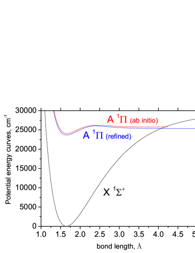
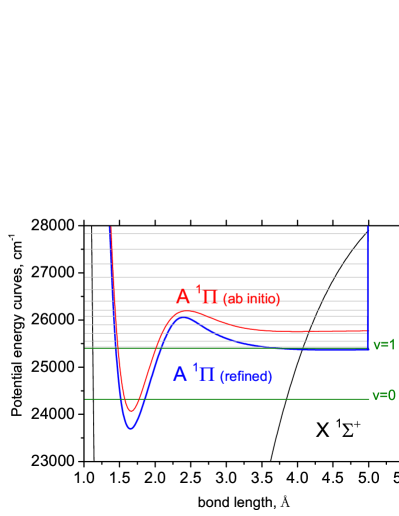
Figure 1: AlH $X\,{}^{1}\Sigma^{+}$ and $A\,{}^{1}\Pi$ state potential energy curves. The zoomed figure (left) also shows the AlH vibrational states and Duo vibrational basis functions, see text for details.

Given the shallow nature of the $A$ curve which also appears to undergo an avoided crossing we decided to perform our own calculations using a high level of electronic structure theory. Ab initio PECs and Dipole Moment Curves (DMCs) were computed using the MOLPRO electronic structure package (Werner et al., 2012) at the multi-reference configuration interaction (MRCI) level using an aug-cc-pV5Z Gaussian basis set. Calculations were performed at 120 bond lengths over the range of $r$ = 2 to 8 a₀. Figure 1 shows the ab initio PEC of $A\,{}^{1}\Pi$, which only supports two bound vibrational states. It also shows a maximum at about 4.5 $a_{0}$ which is probably associated with an avoided crossing. Figure 2 shows our ab initio DMCs, which agree well with the ab initio dipole moment values from Bauschlicher & Langhoff (1988), although, as discussed below, the magnitude of our transition dipole is slightly smaller. Our calculations give a permanent dipole moment of 0.158 D (absolute value) at $r=1.646$ Å at equilibrium, which is slightly higher than that by Bauschlicher & Langhoff (1988), 0.12 D. This is significantly less than the absolute value of 0.186 used by CDMS (Müller et al., 2005), which is taken from an old calculation by Meyer & Rosmus (1975). We also note that the $X$ dipole also changes sign close to equilibrium. We return to these issues below. Matos et al. (1988) in their ab initio work showed a strong variation of the dipole and obtain a value of 0.3 D for $\mu_{0}$ (i.e. a vibrational averaged in the ground vibrational state), while our value is 0.248 D. No experimental values exist. The $A\,{}^{1}\Pi$ – $X\,{}^{1}\Sigma^{+}$ transition dipole moment of AlH also undergoes a change in behaviour in the region around 4.5 $a_{0}$.

In order to represent the complex shape of the shallow $A\,{}^{1}\Pi$ potential energy curve (see Fig. 1), we used a diabatic-like scheme, where the effect of the avoided crossing is described by a $2\times 2$ matrix:

$$\underline{B}=\left(\begin{array}[]{cc}V_{1}(r)&W(r)\\ W(r)&V_{2}(r)\end{array}\right).$$ (6)

Here $V_{1}(r)$ is given by the EMO potential function in Eq. (1), while $V_{2}(r)$ is represented by a simple repulsive form

$$V_{2}(r)=\frac{w_{6}}{r^{6}}.$$

The coupling $W(r)$ is given by

$$W(r)=W_{0}+\frac{\sum_{i\geq 0}w_{i}(r-r_{\rm cr})^{i}}{\cosh[\beta(r-r_{\rm cr})]},$$ (7)

where $r_{\rm cr}$ is a crossing point. The two eigenvalues of $\underline{B}$ are given by

$$V_{\rm low}(r) = \frac{V_{1}(r)+V_{2}(r)}{2}-\frac{\sqrt{[V_{1}(r)-V_{2}(r)]^{2}+4\,W^{2}(r)}}{2},$$ (8)

$$V_{\rm upp}(r) = \frac{V_{1}(r)+V_{2}(r)}{2}+\frac{\sqrt{[V_{1}(r)-V_{2}(r)]^{2}+4\,W^{2}(r)}}{2},$$ (9)

where the lowest root $V_{\rm low}(r)$ corresponds to the $A\,{}^{1}\Pi$ adiabatic PEC.

Initially, the expansion parameters representing this form were obtained by fitting to the ab initio $A$-state PEC shown in Fig. 1 and then refined by fitting to the MARVEL energies. Currently Duo does not support quasi-bound or continuum solutions, see Yurchenko et al. (2016). Technically, by virtue of the sinc DVR (discrete variable representation) method used by Duo to solve the vibrational ($J=0$) Schrödinger equation, Duo uses infinite walls at each end of the integration grid (0.5 – 5.0 Å in our case) as boundary conditions, which is illustrated in Fig. 1. For the $A\,{}^{1}\Pi$ state, we selected 20 basis functions generated by solving the $J=0$ problem for the PEC of the $A\,{}^{1}\Pi$ state using the sinc DVR method (and 60 vibration basis functions for $X\,{}^{1}\Sigma^{+}$). All these basis set functions have zeros at the boundaries, $r=$0.5 and 5.0 Å, and thus represent bound wavefunctions. Therefore the solution of the coupled rovibronic Schrödinger equations with this basis set contains a mixture of real $A\,{}^{1}\Pi$ bound states ($v=0$ and $v=1$) and a large number of continuum states. The corresponding energies of these states for $J=0$ are shown in Fig. 1 as horizontal lines. From these solutions only the $v=0$ and $v=1$ states are actually bound and thus selected for the final line list. The bound states can be easily distinguished from the quasi- or unbound states using the $A$–$X$ transition probabilities or lifetimes, which differ by 3–4 orders of magnitude. It should be noted that the $A\,{}^{1}\Pi$ computed energies suffer from accidental resonances at higher values of $J$ between bound and unbound states, which affect the accuracy of the calculated $v=0$ and $v=1$ energies. As shown below, this is partly resolved by replacing the theoretical energies with the experimentally derived (MARVEL) values.

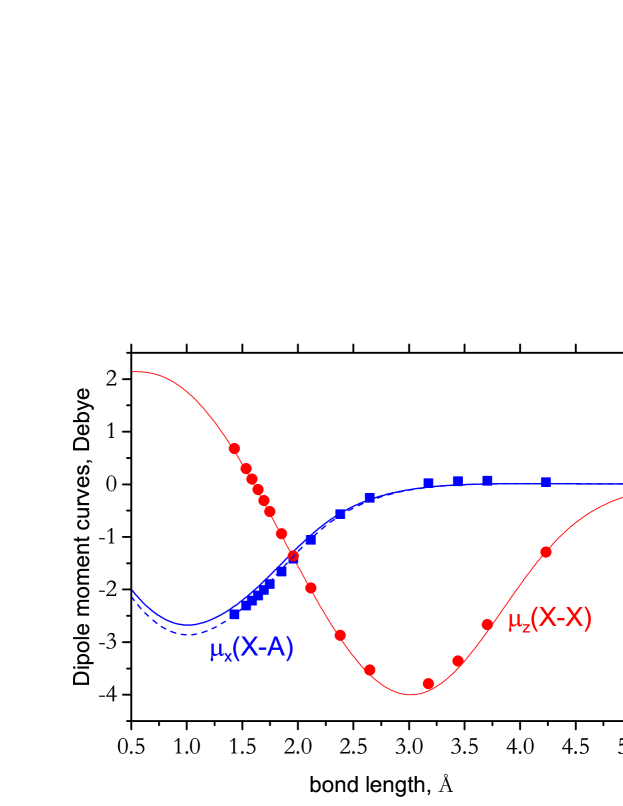
Figure 2: Ab initio (transition) dipole moment curves for AlH, $X$–$X$ and $A$ – $X$: The solid lines are from this work and the symbols represent the dipoles of Bauschlicher & Langhoff (1988); the dashed curve is a scaled version of our ab initio transtion dipole, see text for details.

The BOB-correction in the form given in Eq. (5) was used for the $A$-state as well. In these fits the $X$-state parameters were fixed to the values obtained using Level. The BOB-curves are shown in Fig. 3.

In order to account for the $\Lambda$-doubling effect, we also used an empirical electronic angular momentum (EAM) coupling between the $A\,{}^{1}\Pi$ and $X\,{}^{1}\Sigma^{+}$ states, which was represented by

$$H^{\rm EAM}(R)=(1-\xi)A_{0}^{\rm EAM},$$ (11)

which is nothing else than Eq. (5) truncated after the leading term. The final value of $A_{0}^{\rm EAM}$ is 0.1475 cm^-1 and the EAM curve is shown in Fig. 3.

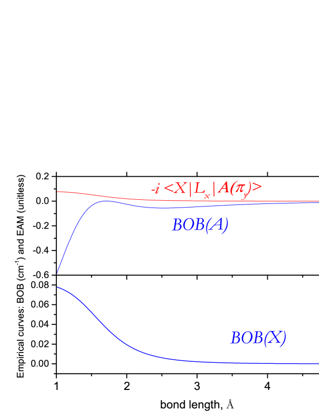
Figure 3: Empirical curves for AlH: Born-Openheimer Breakdown (BOB) for the $X\,{}^{1}\Sigma^{+}$ and $A\,{}^{1}\Pi$ states, plus the $L_{x}$ electronic angular momentum coupling between the two states.

The final fit gave an observed minus calculated root-mean-square (rms) error of 0.025 cm^-1, when compared to our MARVEL energy levels for the $X\,{}^{1}\Sigma^{+}$ state. The MARVEL energy levels of the $A\,{}^{1}\Pi$ state are reproduced with an rms error of 0.59 cm^-1.

Baltayan & Nedelec (1979) reported AlH dissociation energies measured using a hollow cathode discharge by dye laser excitation, 3.16 $\pm 0.01$ eV and 0.24 $\pm 0.01$ eV for the $X\,{}^{1}\Sigma^{+}$ and $A\,{}^{1}\Pi$ states, respectively. The dissociation energy ($D_{\rm e}$) of our empirical PEC of the $X\,{}^{1}\Sigma^{+}$ state is 3.644 eV which overestimates the experimental value. This should not be a problem for our line list since the contributions from the highly excited vibrational states of $X\,{}^{1}\Sigma^{+}$  is practically zero at such energies. For the $A\,{}^{1}\Pi$ PEC we obtained $D_{\rm e}$ = 0.209 eV (ab initio) and 0.210 eV (refined PEC), which compare well to the experimental value by Baltayan & Nedelec (1979). It should be noted that Bauschlicher & Langhoff (1988) also reported ab initio FCI dissociation energies which coincide with the experimental values by Baltayan & Nedelec (1979).

Since the current version of Duo does not account for the isotopic-effect explicitly and thus is not capable of treating a mass-independent model as, for example, in Level, we had to create independent models for different isotopologues. Therefore the same fitting procedure was repeated for AlD, where the model curves were fitted to the AlD experimentally derived energies (MARVEL). Fortunately, the experimental data set for AlD is almost as large as that for AlH.

Final parameters for all the curves representing our two spectroscopic models for AlH and AlD (PECs, DMCs, and other empirical curves) and used in Duo are given in the supplementary material in the form of the Duo input. The program Duo is freely available via the www.exomol.com web site. The actual curves can be extracted from the Duo outputs, which are also provided.

2.3 Lifetimes

The lifetimes of AlH in the $A\,{}^{1}\Pi$ state were measured by Baltayan & Nedelec (1979) using a hollow cathode discharge by dye laser excitation, who reported two values: 66$\pm 4$ ns ($v=0,J=7$) and 83$\pm 6$ ($v=1,J=5$). Using our Einstein coefficients and program ExoCross (Yurchenko et al., 2018a) we obtained 73.64  ns and 102.53 ns for these states, respectively. These lifetimes can also be compared to theoretical values given by Bauschlicher & Langhoff (1988) of 64.3 ns and 96.6 ns, respectively. Our lifetimes are about 1.12 times higher than experiment, which indicates that our transition dipole moment $A$–$X$ is about 1.07 times too strong. Considering that the $A$–$X$ curve by Bauschlicher & Langhoff (1988) is also the same factor larger, see in Fig. 2, we have decided to scale our ab initio transition dipole moment $A$–$X$ by 1.07 up. The resulted transition dipole moment is shown in Fig. 2, where it matches better the ab initio TDMC by Bauschlicher & Langhoff (1988). Using the scaled TDMC, we also obtain a better match for the lifetimes: 64.3 ns ($v=0,J=7$) and 89.6 ($v=1,J=5$). This transition DMC is put forward to produce the AlH line lists.

Figure 4 shows our lifetimes of the $v=0$ and $v=1$ ($A$) rovibronic states of AlH using the scaled DMC. The oscillations in the $v=1$ progression is probably due to accidental resonances with unbound states (see below).

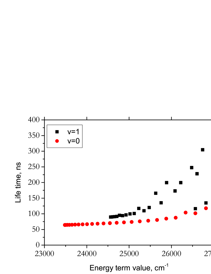
Figure 4: Lifetimes of AlH in the $A\,{}^{1}\Pi$ state.

2.4 Line list generation

Line lists for AlH and AlD were generated using the program Duo.

In order to reduce the numerical noise in the intensity calculations of high overtones characterized by small transition probabilities in the spectra of the $X\,{}^{1}\Sigma^{+}$ state (see recent recommendations by Medvedev et al. (2016)) the DMCs are represented analytically. We use the following expansion (Prajapat et al., 2017; Yurchenko et al., 2018b):

$$\mu(r)=\sum^{N}_{k=0}\mu_{k}\,z^{k}(1-\xi_{p}),$$ (12)

where $z$ is the damped-coordinate given by:

$$z=(r-r_{\rm ref})\,e^{-\beta_{2}(r-r_{\rm ref})^{2}-\beta_{4}(r-r_{\rm ref})^{4}}.$$ (13)

Here $r_{\rm ref}$ is a reference position equal to $r_{\rm e}$ by default and $\beta_{2}$ and $\beta_{4}$ are damping factors. The expansion parameters are given in the supplementary material. As an additional measure to reduce numerical noise in the overtone intensities, a dipole moment cutoff of $10^{-7}$ D was applied to the vibrational dipole moments: all transitions for which the vibrational dipole moments are smaller than $10^{-7}$ D were ignored.

The $A\,{}^{1}\Pi$ – $X\,{}^{1}\Sigma^{+}$ (bound) spectrum only contains transitions to/from the upper states $v^{\prime}=0$ and $v^{\prime}=1$, i.e. no overtones, and thus should not suffer from the numerical noise issue as much as the $X\,{}^{1}\Sigma^{+}$ – $X\,{}^{1}\Sigma^{+}$ band. Therefore the $A\,{}^{1}\Pi$–$X\,{}^{1}\Sigma^{+}$ transition dipole moment was given directly in the (scaled) ab initio grid representation of 120 points. The latter points are interpolated by Duo onto the sinc DVR grid using the cubic splines method (see Yurchenko et al. (2016) for details).

Only bound vibrational and rotational states were retained which meant for ²⁷AlH considering $J\leq 82$ for the $X\,{}^{1}\Sigma^{+}$ state and $J\leq 25$ for the $A\,{}^{1}\Pi$ state. For ²⁷AlD the range of $J$ was increased to $J_{\rm max}=$ 108 and $35$, respectively. Duo input files used to generate the line lists are included as part of the supplementary data. This procedure was then simply repeated for ²⁶AlH by changing the mass of Al and nuclear statistics factor from 12 to 22. All $A\,{}^{1}\Pi$  empirical energies in the .states file of ²⁷AlH were replaced by the MARVEL values, or by values generated using PGOPHER from the constants by Szajna et al. (2015) if the MARVEL energies were not available; for ²⁷AlD we used the experimentally derived term values by Szajna et al. (2015).

The line lists are stored in the standard ExoMol format (Tennyson et al., 2016b) which involves a states file listing all the levels and a transitions file giving the Einstein A coefficients for each transition. The ²⁷AlH line list contains 1,551 states and 39,483 transitions; the ²⁷AlD line list contains 2,930 states and 85,494 transitions; The ²⁶AlH line list contains 1,549 states and 35,910 transitions.

Tables 2 and 3 give samples of these files. Full versions can be found at CDS, via ftp://cdsarc.u-strasbg.fr/pub/cats/J/MNRAS/, or http://cdsarc.u-strasbg.fr/viz-bin/qcat?J/MNRAS/, or from www.exomol.com.

Table 2: Extract from the state file for ²⁷Al¹H. Full tables are available from http://cdsarc.u-strasbg.fr/cgi-bin/VizieR?-source=J/MNRAS/xxx/yy and www.exomol.com.

$n$	Energy (cm-1)	$g_{i}$	$J$	$\tau$	Parity	e/f	State	$v$	${\Lambda}$	${\Sigma}$	$\Omega$
1	0.000000	12	0	inf	+	e	X1Sigma+	0	0	0	0
2	1625.069321	12	0	4.9283E-03	+	e	X1Sigma+	1	0	0	0
3	3194.213685	12	0	2.6224E-03	+	e	X1Sigma+	2	0	0	0
4	4708.817022	12	0	1.8630E-03	+	e	X1Sigma+	3	0	0	0
5	6170.193041	12	0	1.4908E-03	+	e	X1Sigma+	4	0	0	0
6	7579.564189	12	0	1.2739E-03	+	e	X1Sigma+	5	0	0	0
7	8938.046805	12	0	1.1350E-03	+	e	X1Sigma+	6	0	0	0
8	10246.644027	12	0	1.0410E-03	+	e	X1Sigma+	7	0	0	0
9	11506.245734	12	0	9.7519E-04	+	e	X1Sigma+	8	0	0	0
10	12717.633797	12	0	9.2834E-04	+	e	X1Sigma+	9	0	0	0

$n$: State counting number.

$\tilde{E}$: State energy in cm^-1.

$g_{i}$: Total statistical weight, equal to ${g_{\rm ns}(2J+1)}$.

$J$: Total angular momentum.

$\tau$: Lifetime (s^-1).

$+/-$: Total parity.

$e/f$: Rotationless parity.

State: Electronic state.

$v$: State vibrational quantum number.

$\Lambda$: Projection of the electronic angular momentum.

$\Sigma$: Projection of the electronic spin.

$\Omega$: Projection of the total angular momentum, $\Omega=\Lambda+\Sigma$.

Table 3: Extracts from the transitions file for ²⁷AlH. Full tables are available from http://cdsarc.u-strasbg.fr/cgi-bin/VizieR?-source=J/MNRAS/xxx/yy and www.exomol.co.

$F$	$I$	$A_{FI}$	$\tilde{\nu}_{FI}$
1075	1087	0.5502E-09	47.949528
1529	1488	1.5634E-11	47.965895
561	520	6.1183E-02	47.984746
218	176	0.6544E-09	48.007351
1415	1384	1.4996E-11	48.171601
441	399	1.1015E-01	48.615068
198	156	0.8765E-09	48.846517
198	156	3.0699E-03	48.846517

$F$: Upper state counting number;

$I$: Lower state counting number;

$A_{FI}$: Einstein A coefficient in s^-1.

$\tilde{\nu}_{FI}$: Energy term value in cm^-1.

3 Results

3.1 Partition function

Partition functions were generated for each isotopologue by explicit summation of the energy levels. Comparison for ²⁷AlH with the recent results of Barklem & Collet (2016) and with the partition function generated using parameters from Sauval & Tatum (1984) shows excellent agreement for temperatures below 5000 K (see Fig. 5) once allowance is made for the fact that ExoMol adopts the HITRAN convention (Gamache et al., 2017) which includes the full nuclear spin degeneracy factor in the partition function (12 in case of ²⁷AlH, 18 in case of ²⁷AlD and 22 in case of ²⁶AlH).

It should be noted that AlH is unlikely to be important at temperatures above 5000 K.

Partition functions, $Q(T)$, on a 1 K grid up to 5000 K are given for each isotopologue in the supplementary material. For ease of use we also provide fits in the form proposed by Vidler & Tennyson (2000):

$$\log_{10}Q(T)=\sum_{n=0}^{6}a_{n}\left[\log T\right]^{n}$$ (14)

with the values given in Table 4.

Table 4: Fitting parameters used to represent the partition functions, see eq. (14). Fits are valid for temperatures up to 5000 K.

Parameter	27AlH	27AlD	26AlH
$a_{0}$	$1.07862304206$	$1.25534381874$	$1.34186025327$
$a_{1}$	$0.38191971276$	$0.22993489470$	$0.38228272653$
$a_{2}$	$-2.22562466705$	$-1.92470848538$	$-2.22605038250$
$a_{3}$	$4.34557816661$	$6.16172026680$	$4.34313450679$
$a_{4}$	$-3.62598781682$	$-7.66641279825$	$-3.62196458297$
$a_{5}$	$1.71637190159$	$5.35122144723$	$1.71374588820$
$a_{6}$	$-0.47932820561$	$-2.24207082067$	$-0.47845359880$
$a_{7}$	$0.07359563236$	$0.55715405704$	$0.07344763428$
$a_{8}$	$-0.00476226937$	$-0.07543604728$	$-0.00475215090$
$a_{9}$		$0.00427936817$

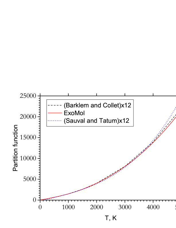
Figure 5: Temperature dependence of the partition function of AlH computed using our line lists and compared to those by Sauval & Tatum (1984) and Barklem & Collet (2016).

3.2 Spectra

In the following, we present different spectra of AlH computed using the new line lists and utilizing the program ExoCross (Yurchenko et al., 2018a). Figure 6 gives an overview of the AlH line list in the form of absorption cross sections for a range of temperatures from 300 to 3000 K.

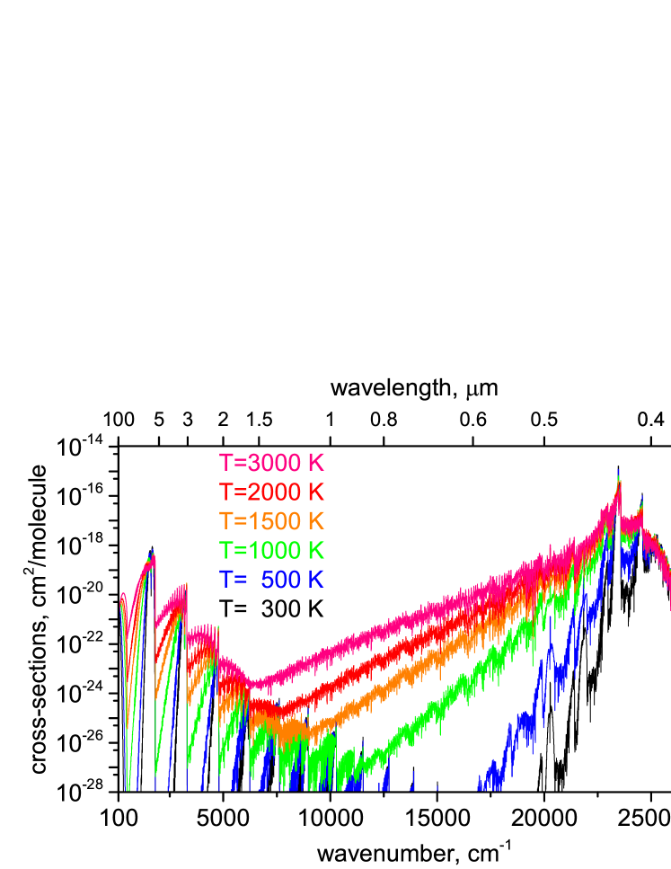
Figure 6: Temperature dependence of the AlH absorption spectrum using the Gaussian profile with HWHM=5 cm^-1. The absorption profile becomes flatter with increasing temperature.

Our line lists can be used to generate spectra for a variety of conditions. First we compare with available laboratory spectra. Figure 7 compares an emission infrared spectrum of AlH recorded by White et al. (1993) with that generated using our line list assuming a temperature of 1700 K. Although the experimental spectrum does not provide the absolute scale for the intensities, there is good agreement for the relative intensities of the hot bands in this region between the experiment and our predictions. Our R-branch appears to be slightly stronger relative to the P-branch than the observations of White et al. (1993), but given the variable baseline and presence of self-absorption in the observed spectrum this may not be significant.

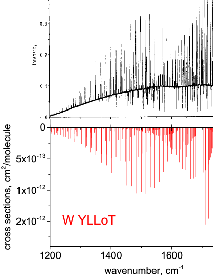
Figure 7: Infrared spectrum of AlH by White et al. (1993) (upper) compared to the emission spectrum computed using our line list assuming a temperature of 1700 K and a Gaussian profile with the HWHM of 0.01 cm^-1. Reproduced from White et al. (1993), with the permission of AIP Publishing.

Figure 8 shows a comparison with the emission 0–0 and 1–1 bands of the $A\,{}^{1}\Pi$ – $X\,{}^{1}\Sigma^{+}$ system of AlH and AlD by Szajna et al. (2015). The observed spectrum was produced from an electric discharge in an aluminium hollow-cathode lamp. Our spectrum has been synthesized assuming a vibrational temperature of 4500 K and rotational temperature of 900 K. Comparisons with the figure suggest that the experiments had an even lower effective rotational temperature and a higher effective vibrational temperature. Inspection of Fig. 8 suggests that our 1–1 band is blue-shifted relative to the experiment by about 7  cm^-1. Our actual numerical agrement is much better (within experimental uncertainly), which suggest some problems with the original figure from this paper.

Figure 9 illustrate a good agreement of the theoretical emission spectrum of the $A\,{}^{1}\Pi$ – $X\,{}^{1}\Sigma^{+}$  band $(1,0)$ at $T=600$ K of AlD with the experiment by Szajna et al. (2017a).

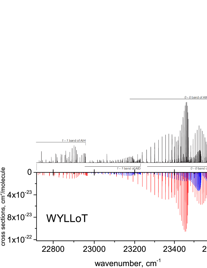
Figure 8: Comparison between the 0–0 and 1–1 bands of the $A\,{}^{1}\Pi$ – $X\,{}^{1}\Sigma^{+}$ emission spectrum of AlH and AlD measured by Szajna et al. (2015) (upper) and computed using our line list (lower) assuming a temperature of 4500 K (vibrational) and 900 K (rotational). The intensities of the AlD theoretical spectrum, given in blue and annotated in the experimental spectrum, are scaled by a factor 0.5. Reprinted from Szajna et al. (2015), Copyright (2015), with permission from Elsevier.

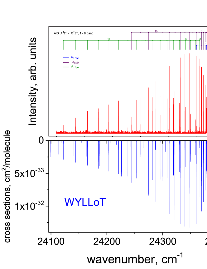
Figure 9: Comparison between the 1–0 band of the $A\,{}^{1}\Pi$ – $X\,{}^{1}\Sigma^{+}$ emission spectrum of AlD measured by Szajna et al. (2017a) (upper) and computed using our line list assuming a temperature of 600 K. Reprinted from Szajna et al. (2017a), Copyright (2017), with permission from Elsevier.

Rice et al. (1992) reported experimentally determined ratios of Einstein coefficients for a number of vibrational bands of $A\,{}^{1}\Pi$ – $X\,{}^{1}\Sigma^{+}$, which we use to assess our transition probabilities in Table 5. Our ratios are found to be in excellent agreement with experiment.

Table 5: $A\,{}^{1}\Pi$ – $X\,{}^{1}\Sigma^{+}$ Einstein coefficients $A_{v^{\prime}v^{\prime\prime}}$ (s^-1) compared to experimentally-derived ratios from Rice et al. (1992), where we used $J^{\prime}=1$ and $J^{\prime\prime}=0$.

	This work	Exp.
$A_{00}$	$9028000$
$A_{01}$	$3878$
$A_{10}$	$810100$
$A_{12}$	$165900$
$A_{11}$	$5407000$
$A_{01}/A_{00}$	$0.00043$	$0.0018\pm 0.0001$
$A_{12}/A_{11}$	$0.03068$	$0.029\pm 0.004$
$A_{10}/A_{11}$	$0.14982$	$0.15\pm 0.02$

Finally, Figure 10 gives a comparison with the long-wavelength, rotational spectrum taken from the CDMS database (Müller et al., 2005). The agreement between the line positions is excellent, although we recommend using the highly-accurate CDMS frequency directly for long-wavelength studies of cool sources. However, there is approximately a factor of two discrepancy in the predicted line intensities. This difference is almost exactly in line with the square of the ratio of our dipole to that of Meyer & Rosmus (1975) used by CDMS. Our vibrationally averaged value for the ground state of AlH is $0.248$ D, which is significantly different from the permanent $\mu_{\rm e}$ value 0.158 D. We would recommend that CDMS adopts our value in future and note that using this value will approximately double the upper limit for AlH in IRC+10216 determined by Cernicharo et al. (2010).

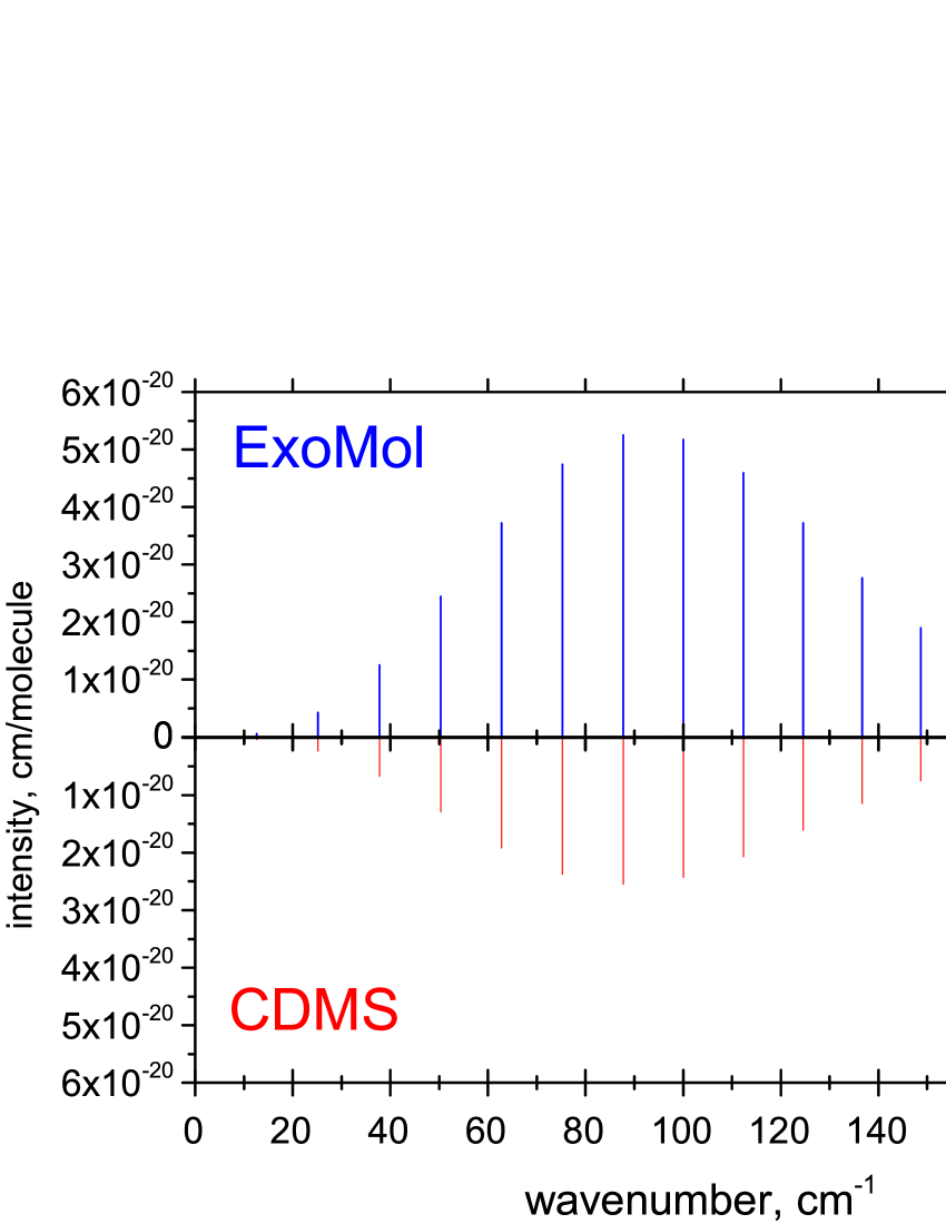
Figure 10: Comparison between pure rotational spectrum of ²⁷AlH at 298 K given by CDMS (Müller et al., 2005) (lower) and computed using our line list (upper).

4 Conclusions

Line lists for three AlH isotopologue species were computed using a mixture of empirical and ab initio curves representing our spectroscopic model. The programs Level (Le Roy, 2017) and Duo (Yurchenko et al., 2016) were used to obtain the empirical curves, while Duo was used for the line list production. The partition functions and lifetimes were computed using the program ExoCross (Yurchenko et al., 2018a).

We provide comprehensive line lists for AlH isotopologue species which can be downloaded from the CDS, via ftp://cdsarc.u-strasbg.fr/pub/cats/J/MNRAS/, or http://cdsarc.u-strasbg.fr/viz-bin/qcat?J/MNRAS/, or from www.exomol.com.

References

- Allard (2014) Allard F., 2014, in IAU Symposium, Vol. 299, IAU Symposium, Booth M., Matthews B. C., Graham J. R., eds., pp. 271–272
- Baltayan & Nedelec (1979) Baltayan P., Nedelec O., 1979, J. Chem. Phys., 70, 2399
- Barklem & Collet (2016) Barklem P. S., Collet R., 2016, A&A, 588, A96