Regression with Comparisons: Escaping the Curse of Dimensionality with Ordinal Information

Abstract

In supervised learning, we typically leverage a fully labeled dataset to design methods for function estimation or prediction. In many practical situations, we are able to obtain alternative feedback, possibly at a low cost. A broad goal is to understand the usefulness of, and to design algorithms to exploit, this alternative feedback. In this paper, we consider a semi-supervised regression setting, where we obtain additional ordinal (or comparison) information for the unlabeled samples. We consider ordinal feedback of varying qualities where we have either a perfect ordering of the samples, a noisy ordering of the samples or noisy pairwise comparisons between the samples. We provide a precise quantification of the usefulness of these types of ordinal feedback in both nonparametric and linear regression, showing that in many cases it is possible to accurately estimate an underlying function with a very small labeled set, effectively escaping the curse of dimensionality. We also present lower bounds, that establish fundamental limits for the task and show that our algorithms are optimal in a variety of settings. Finally, we present extensive experiments on new datasets that demonstrate the efficacy and practicality of our algorithms and investigate their robustness to various sources of noise and model misspecification.

Keywords: Pairwise Comparison, Ranking, Regression, Interactive Learning

1 Introduction

Classical regression is centered around the development and analysis of methods that use labeled observations, $\{(X_{1},y_{1}),\ldots,(X_{n},y_{n})\}$, where each $(X_{i},y_{i})\in\mathbb{R}^{d}\times\mathbb{R}$, in various tasks of estimation and inference. Nonparametric and high-dimensional methods are appealing in practice owing to their flexibility, and the relatively weak a-priori structural assumptions that they impose on the unknown regression function. However, the price we pay is that these methods typically require a large amount of labeled data to estimate complex target functions, scaling exponentially with the dimension for fully nonparametric methods and scaling linearly with the dimension for high-dimensional parametric methods – the so-called curse of dimensionality. This has motivated research on structural constraints – for instance, sparsity or manifold constraints – as well as research on active learning and semi-supervised learning where labeled samples are used judiciously.

We consider a complementary approach, motivated by applications in material science, crowdsourcing, and healthcare, where we are able to supplement a small labeled dataset with a potentially larger dataset of ordinal information. Such ordinal information is obtained either in the form of a (noisy) ranking of unlabeled points or in the form of (noisy) pairwise comparisons between function values at unlabeled points. Some illustrative applications of the methods we develop in this paper include:

Example 1: Crowdsourcing. In crowdsourcing we rely on human labeling effort, and in many cases humans are able to provide more accurate ordinal feedback with substantially less effort (see for instance Tsukida and Gupta (2011); Shah et al. (2016a, c)). When crowdsourced workers are asked to give numerical price estimates, they typically have difficulty giving a precise answer, resulting in a high variance between worker responses. On the other hand, when presented two products or listings side by side, workers may be more accurate at comparing them. We conduct experiments on the task of price estimation in Section 4.4.

Example 2: Material Synthesis. In material synthesis, the broad goal is to design complex new materials and machine learning approaches are gaining popularity (Xue et al., 2016; Faber et al., 2016). Typically, given a setting of input parameters (temperature, pressure etc.) we are able to perform a synthesis experiment and measure the quality of resulting synthesized material. Understanding this landscape of material quality is essentially a task of high-dimensional function estimation. Synthesis experiments can be costly and material scientists when presented with pairs of input parameters are often able to cheaply and reasonably accurately provide comparative assessments of quality.

Example 3: Patient Diagnosis. In clinical settings, precise assessment of each individual patient’s health status can be difficult, expensive, and risky but comparing the relative status of two patients may be relatively easy and accurate.

In each of these settings, it is important to develop methods for function estimation that combine standard supervision with (potentially) cheaper and abundant ordinal or comparative supervision.

1.1 Our Contributions

We consider both linear and nonparametric regression with both direct (cardinal) and comparison (ordinal) information. In both cases, we consider the standard statistical learning setup, where the samples $X$ are drawn i.i.d. from a distribution $\mathbb{P}_{X}$ on $\mathbb{R}^{d}$. The labels $y$ are related to the features $X$ as,

$$y=f(X)+\varepsilon,$$

where $f=\mathbb{E}[y|X]$ is the underlying regression function of interest, and $\varepsilon$ is the mean-zero label noise. Our goal is to construct an estimator $\widehat{f}$ of $f$ that has low risk or mean squared error (MSE),

$$R(\widehat{f},f)=\mathbb{E}(\widehat{f}(X)-f(X))^{2},$$

where the expectation is taken over the labeled and unlabeled training samples, as well as a new test point $X$. We also study the fundamental information-theoretic limits of estimation with classical and ordinal supervision by establishing lower (and upper) bounds on the minimax risk. Letting $\eta$ denote various problem dependent parameters, which we introduce more formally in the sequel, the minimax risk:

$$\mathfrak{M}(m,n;\eta)=\inf_{\widehat{f}}\sup_{f\in\mathcal{F}_{\eta}}R(\widehat{f},f),$$ (1)

provides an information-theoretic benchmark to assess the performance of an estimator.

First, focusing on nonparametric regression, we develop a novel Ranking-Regression (R²) algorithm for nonparametric regression that can leverage ordinal information, in addition to direct labels. We make the following contributions:

• To establish the usefulness of ordinal information in nonparametric regression, in Section 2.2 we consider the idealized setting where we obtain a perfect ordering of the unlabeled set. We show that the risk of the R² algorithm can be bounded with high-probability as $\widetilde{O}(m^{-2/3}+n^{-2/d})$, where $m$ denotes the number of labeled samples and $n$ the number of ranked samples. To achieve an MSE of $\varepsilon$, the number of labeled samples required by R² is independent of the dimensionality of the input features. This result establishes that sufficient ordinal information of high quality can allow us to effectively circumvent the curse of dimensionality.

• In Sections 2.3 and 2.4 we analyze the R² algorithm when using either a noisy ranking of the samples or noisy pairwise comparisons between them. For noisy ranking, we show that the MSE is bounded by $\widetilde{O}(m^{-2/3}+\sqrt{\nu}+n^{-2/d})$, where $\nu$ is the Kendall-Tau distance between the true and noisy ranking. As a corollary, we combine R² with algorithms for ranking from pairwise comparisons (Braverman and Mossel, 2009) to obtain an MSE of $\widetilde{O}(m^{-2/3}+n^{-2/d})$ when $d\geq 4$, when the comparison noise is bounded.

Turning our attention to the setting of linear regression with ordinal information, we develop an algorithm that uses active (or adaptive) comparison queries in order to reduce both the label complexity and total query complexity.

• In Section 3 we develop and analyze an interactive learning algorithm that estimates a linear predictor using both labels and comparison queries. Given a budget of $m$ label queries and $n$ comparison queries, we show that MSE of our algorithm decays at the rate of $\widetilde{O}\left(1/m+\exp(-n/d)\right)$. Once again we see that when sufficiently many comparisons are available, the label complexity of our algorithm is independent of the dimension $d$.

To complement these results we also give information-theoretic lower bounds to characterize the fundamental limits of combining ordinal and standard supervision.

• For nonparametric regression, we show that the R² algorithm is optimal up to log factors both when it has access to a perfect ranking, as well as when the comparisons have bounded noise. For linear regression, we show that the rate of $O(1/m)$, and the total number of queries, are not improvable up to log factors.

On the empirical side we comprehensively evaluate the algorithms we propose, on simulated and real datasets.

• We use simulated data, and study the performance of our algorithms as we vary the noise in the labels and in the ranking.

• Second, we consider a practical application of predicting people’s ages from photographs. For this dataset we obtain comparisons using people’s apparent ages (as opposed to their true biological age).

• Finally, we curate a new dataset using crowdsourced data obtained through Amazon’s Mechanical Turk. We provide workers AirBnB listings and attempt to estimate property asking prices. We obtain both direct and comparison queries for the listings, and also study the time taken by workers to provide these different types of feedback. We find that, our algorithms which combine direct and comparison queries are able to achieve significantly better accuracy than standard supervised regression methods, for a fixed time budget.

1.2 Related Work

As a classical way to reduce the labeling effort, active learning has been mostly focused on classification (Hanneke, 2009). For regression, it is known that, in many natural settings, the ability to make active queries does not lead to improved rates over passive baselines. For example, Chaudhuri et al. (2015) shows that when the underlying model is linear, the ability to make active queries can only improve the rate of convergence by a constant factor, and leads to no improvement when the feature distribution is spherical Gaussian. In Willett et al. (2006), the authors show a similar result that in nonparametric settings, active queries do not lead to a faster rate for smooth regression functions except when the regression function is piecewise smooth.

There is considerable work in supervised and unsupervised learning on incorporating additional types of feedback beyond labels. For instance, Zou et al. (2015); Poulis and Dasgupta (2017) study the benefits of different types of “feature feedback” in clustering and supervised learning respectively. Dasgupta and Luby (2017) consider learning with partial corrections, where the user provides corrective feedback to the algorithm when the algorithm makes an incorrect prediction. Ramaswamy et al. (2018) consider multiclass classification where the user can choose to abstain from making predictions at a cost.

There is also a vast literature on models and methods for analyzing pairwise comparison data (Tsukida and Gupta, 2011; Agarwal et al., 2017), like the classical Bradley-Terry (Bradley and Terry, 1952) and Thurstone (Thurstone, 1927) models. In these literature, the typical focus is on ranking or quality estimation for a fixed set of objects. In contrast, we focus on function estimation and the resulting models and methods are quite different. We build on the work on “noisy sorting” (Braverman and Mossel, 2009; Shah et al., 2016b) to extract a consensus ranking from noisy pairwise comparisons.

Perhaps the closest in spirit to this work are the two recent papers (Kane et al., 2017; Xu et al., 2017) that consider binary classification with ordinal information. These works differ from the proposed approach in their focus on classification, emphasis on active querying strategies and binary-search-based methods.

Given ordinal information of sufficient fidelity, the problem of nonparametric regression is related to the problem of regression with shape constraints, or more specifically isotonic regression (Barlow, 1972; Zhang, 2002). Accordingly, we leverage such algorithms in our work and we comment further on the connections in Section 2.2. Some salient differences between this literature and our work are that we design methods that work in a semisupervised setting, and further that our target is an unknown $d$-dimensional (smooth) regression function as opposed to a univariate shape-constrained function.

The rest of this paper is organized as follows. In Section 2, we consider the problem of combining direct and comparison-based labels for nonparametric regression, providing upper and lower bounds for both noiseless and noisy ordinal models. In Section 3, we consider the problem of combining adaptively chosen direct and comparison-based labels for linear regression. In Section 4, we turn our attention to an empirical evaluation of our proposed methods on real and synthetic data. Finally, we conclude in Section 5 with a number of additional results and open directions. In the Appendix we present detailed proofs for various technical results and a few additional supplementary experimental results.

2 Nonparametric Regression with Ordinal Information

We now provide analysis for nonparametric regression. First, in Section 2.1 we establish the problem setup and notations. Then, we introduce the R² algorithm in Section 2.2 and analyze it under perfect rankings. Next, we analyze its performance for noisy rankings and comparisons in Sections 2.3 and 2.4.

2.1 Background and Problem Setup

We consider a nonparametric regression model with random design, i.e. we suppose first that we are given access to an unlabeled set $\mathcal{U}=\{X_{1},\ldots,X_{n}\}$, where $X_{i}\in\mathcal{X}\subset[0,1]^{d}$, and $X_{i}$ are drawn i.i.d. from a distribution $\mathbb{P}_{X}$ and we assume that $\mathbb{P}_{X}$ has a density $p$ which is upper and lower bounded as $0<p_{\min}\leq p(x)\leq p_{\max}$ for $x\in\mathcal{X}$. Our goal is to estimate a function $f:\mathcal{X}\mapsto\mathbb{R}$, where following classical work (Györfi et al., 2006; Tsybakov, 2009) we assume that $f$ is bounded in $[-M,M]$ and belongs to a Hölder ball $\mathcal{F}_{s,L}$, with $0<s\leq 1$:

$$\mathcal{F}_{s,L}=\left\{f:|f(x)-f(y)|\leq L\|x-y\|_{2}^{s},\forall~{}x,y\in\mathcal{X}\right\}.$$

For $s=1$ this is the class of Lipschitz functions. We discuss the estimation of smoother functions (i.e. the case when $s>1$) in Section 5. We obtain two forms of supervision:

1. Classical supervision: For a (uniformly) randomly chosen subset $\mathcal{L}\subseteq\mathcal{U}$ of size $m$ (we assume throughout that $m\leq n$ and focus on settings where $m\ll n$) we make noisy observations of the form:

   $$y_{i}=f(X_{i})+\epsilon_{i},~{}~{}i\in\mathcal{L},$$

   $\text{where }\epsilon_{i}\text{ are i.i.d.}$ Gaussian with $\mathbb{E}[\epsilon_{i}]=0,\text{Var}[\epsilon_{i}]=1$. We denote the indices of the labeled samples as $\{t_{1},\ldots,t_{m}\}\subset\{1,\ldots,n\}$.

2. Ordinal supervision: For the given dataset $\{X_{1},\ldots,X_{n}\}$ we let $\pi$ denote the true ordering, i.e. $\pi$ is a permutation of $\{1,\ldots,n\}$ such that for $i,j\in\{1,\ldots,n\}$, with $\pi(i)\leq\pi(j)$ we have that $f(X_{i})\leq f(X_{j})$. We assume access to one of the following types of ordinal supervision:

   (1) We assume that we are given access to a noisy ranking $\widehat{\pi}$, i.e. for a parameter $\nu\in[0,1]$ we assume that the Kendall-Tau distance between $\widehat{\pi}$ and the true-ordering is upper-bounded as:

   $$\sum_{i,j\in[n]}\mathbb{I}[(\pi(i)-\pi(j))(\widehat{\pi}(i)-\widehat{\pi}(j))<0]\leq\nu n^{2}.$$ (2)

   (2) For each pair of samples $(X_{i},X_{j})$, with $i<j$ we obtain a comparison $Z_{ij}$ where for some constant $\lambda>0$:

   $$\mathbb{P}(Z_{ij}=\mathbb{I}(f(X_{i})>f(X_{j})))\geq\frac{1}{2}+\lambda.$$ (3)

   As we discuss in Section 2.4, it is straightforward to extend our results to a setting where only a randomly chosen subset of all pairwise comparisons are observed.

Although classic supervised learning learns a regression function with labels only and without ordinal supervision, we note that learning cannot happen in the opposite way: That is, we cannot consistently estimate the underlying function with only ordinal supervision and without labels: the underlying function is only identifiable up to certain monotonic transformations.

As discussed in Section 1.1, our goal is to design an estimator $\widehat{f}$ of $f$ that achieves the minimax mean squared error (1), when $f\in\mathcal{F}_{s,L}$. We conclude this section recalling a well-known fact: given access to only classical supervision the minimax risk $\mathfrak{M}(m;\eta)=\Theta(m^{-\frac{2s}{2s+d}}),$ suffers from an exponential curse of dimensionality.

2.2 Nonparametric Regression with Perfect Ranking

To ascertain the value of ordinal information we first consider an idealized setting, where we are given a perfect ranking $\pi$ of the unlabeled samples in $\mathcal{U}$. We present our Ranking-Regression (R²) algorithm with performance guarantees in Section 2.2.1, and a lower bound for it in Section 2.2.2 which shows that R² is optimal up to log factors.

2.2.1 Upper bounds for the R² Algorithm

Algorithm 1 R²: Ranking-Regression

0:  Unlabeled data $\mathcal{U}=\{X_{1},\ldots,X_{n}\}$, a labeled set of size $m$ and corresponding labels, i.e. samples $\{(X_{t_{1}},y_{t_{1}}),\ldots,(X_{t_{m}},y_{t_{m}})\},$ and a ranking $\widehat{\pi}$.

1:  Order elements in $\mathcal{U}$ as $(X_{\widehat{\pi}(1)},\ldots,X_{\widehat{\pi}(n)})$.

2:  Run isotonic regression (see (4)) on $\{y_{t_{1}},\ldots,y_{t_{m}}\}$. Denote the estimated values by $\{\widehat{y}_{t_{1}},\ldots,\widehat{y}_{t_{m}}\}$.

3:  For $i=1,2,\ldots,n$, let $\widetilde{i}=t_{k}$, where $\widehat{\pi}(t_{k})$ is the largest value such that $\widehat{\pi}(t_{k})\leq\widehat{\pi}(i),k=0,1,\ldots,m$, and $\widetilde{i}=\star$ if no such $t_{k}$ exists. Set

$$\widehat{y}_{i}=\begin{cases}\widehat{y}_{\widetilde{i}}~{}~{}&\text{if}~{}~{}\widetilde{i}\neq\star\\ 0~{}~{}&\text{otherwise}.\end{cases}$$

3:  Function $\widehat{f}=~{}$NearestNeighbor$(\{(X_{i},\widehat{y}_{i})\}_{i=1}^{n})$.

Our nonparametric regression estimator is described in Algorithm 1 and Figure 1. We first rank all the samples in $\mathcal{U}$ according to the (given or estimated) permutation $\widehat{\pi}$. We then run isotonic regression (Barlow, 1972) on the labeled samples in $\mathcal{L}$ to de-noise them and borrow statistical strength. In more detail, we solve the following program to de-noise the labeled samples:

$$\begin{split}&\min_{\{\widehat{y}_{\widehat{\pi}(t_{1})},\ldots,\widehat{y}_{\widehat{\pi}(t_{m})}\}}\sum_{k=1}^{m}(\widehat{y}_{\widehat{\pi}(t_{k})}-y_{\widehat{\pi}(t_{k})})^{2}\\ &~{}~{}~{}~{}~{}~{}\text{s.t. }~{}~{}~{}\widehat{y}_{t_{k}}\leq\widehat{y}_{t_{l}}~{}~{}\forall~{}(k,l)~{}~{}\text{such that}~{}~{}\widehat{\pi}(t_{k})<\widehat{\pi}(t_{l})\\ &~{}~{}~{}~{}~{}~{}~{}~{}~{}~{}~{}~{}~{}~{}-M\leq\{\hat{y}_{\widehat{\pi}(t_{1})},\ldots,\hat{y}_{\widehat{\pi}(t_{m})}\}\leq M.\end{split}$$ (4)

We introduce the bounds $\{M,-M\}$ in the above program to ease our analysis. In our experiments, we simply set $M$ to be a large positive value so that it has no influence on our estimator. We then leverage the ordinal information in $\widehat{\pi}$ to impute regression estimates for the unlabeled samples in $\mathcal{U}$, by assigning each unlabeled sample the value of the nearest (de-noised) labeled sample which has a smaller function value according to $\widehat{\pi}$. Finally, for a new test point, we use the imputed (or estimated) function value of the nearest neighbor in $\mathcal{U}$.

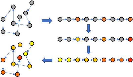
Figure 1: Top Left: A group of unlabeled points are ranked according to function values using ordinal information only. Top Right: We obtain function values of $m$ randomly chosen samples. Middle Right: The values are adjusted using isotonic regression. Bottom Right: Function values of other unlabeled points are inferred. Bottom Left: For a new point, the estimated value is given by the nearest neighbor in $\mathcal{U}$.

In the setting where we use a perfect ranking the following theorem characterizes the performance of R²:

Theorem 1

For constants $C_{1},C_{2}>0$ the MSE of $\widehat{f}$ is bounded by

$$\mathbb{E}(\widehat{f}(X)-f(X))^{2}\leq ~{}C_{1}m^{-2/3}\log^{2}n\log m+C_{2}n^{-2s/d}.$$

Before we turn our attention to the proof of this result, we examine some consequences.
Remarks: (1) Theorem 1 shows a surprising dependency on the sizes of the labeled and unlabeled sets ($m$ and $n$). The MSE of nonparametric regression using only the labeled samples is $\Theta(m^{-\frac{2s}{2s+d}})$ which is exponential in $d$ and makes nonparametric regression impractical in high-dimensions. Focusing on the dependence on $m$, Theorem 1 improves the rate to $m^{-2/3}\text{polylog}(m,n)$, which is no longer exponential. By using enough ordinal information we can avoid the curse of dimensionality.
(2) On the other hand, the dependence on $n$ (which dictates the amount of ordinal information needed) is still exponential. This illustrates that ordinal information is most beneficial when it is copious. We show in Section 2.2.2 that this is unimprovable in an information-theoretic sense.
(3) Somewhat surprisingly, we also observe that the dependence on $n$ is faster than the $n^{-\frac{2s}{2s+d}}$ rate that would be obtained if all the samples were labeled. Intuitively, this is because of the noise in labels: Given the $m$ labels along with the (perfect) ranking, the difference between two neighboring labels is typically very small (around $1/m$). Therefore, any unlabeled points in $\mathcal{U}\setminus\mathcal{L}$ will be restricted to an interval much narrower than the constant noise in direct labels. In the case where all points are labeled (i.e., $m=n$), the MSE is of order $n^{-2/3}+n^{-2s/d}$, also slightly better rate than when no ordinal information is available. On the other hand, the improvement is stronger when $m\ll n$.
(4) Finally, we also note in passing that the above theorem provides an upper bound on the minimax risk in (1).

Proof Sketch We provide a brief outline and defer technical details to the Supplementary Material. For a randomly drawn point $X\in\mathcal{X}$, we denote by $X_{\alpha}$ the nearest neighbor of $X$ in $\mathcal{U}$. We decompose the MSE as

$$\mathbb{E}\left[(\widehat{f}(X)-f(X))^{2}\right]\leq 2\mathbb{E}\left[(\widehat{f}(X)-f(X_{\alpha}))^{2}\right]+2\mathbb{E}\left[(f(X_{\alpha})-f(X))^{2}\right].$$ (5)

The second term corresponds roughly to the finite-sample bias induced by the discrepancy between the function value at $X$ and the closest labeled sample. We use standard sample-spacing arguments (see Györfi et al. (2006)) to bound this term. This term contributes the $n^{-2s/d}$ rate to the final result. For the first term, we show a technical result in the Appendix (Lemma 13). Without loss of generality suppose $f\big{(}X_{t_{1}}\big{)}\leq\cdots f\big{(}X_{t_{m}}\big{)}$. By conditioning on a probable configuration of the points and enumerating over choices of the nearest neighbor we find that roughly (see Lemma 13 for a precise statement):

$$\mathbb{E}\left[(\widehat{f}(X)-f(X_{\alpha}))^{2}\right]\leq\Big{(}\frac{\log^{2}n\log m}{m}\Big{)}\times$$

$$\mathbb{E}\Big{(}\sum_{k=1}^{m}\Big{(}\big{(}\widehat{f}(X_{t_{k}})-f(X_{t_{k}})\big{)}^{2}+\big{(}f\big{(}X_{t_{k+1}}\big{)}-f\big{(}X_{t_{k}}\big{)}\big{)}^{2}\Big{)}\Big{)}.$$ (6)

Intuitively, these terms are related to the estimation error arising in isotonic regression (first term) and a term that captures the variance of the function values (second term). When the function $f$ is bounded, we show that the dominant term is the isotonic estimation error which is on the order of $m^{1/3}$. Putting these pieces together we obtain the theorem.  

2.2.2 Lower bounds with Ordinal Data

To understand the fundamental limits on the usefulness of ordinal information, as well as to study the optimality of the R² algorithm we now turn our attention to establishing lower bounds on the minimax risk. In our lower bounds we choose $\mathbb{P}_{\mathcal{X}}$ to be uniform on $[0,1]^{d}$. Our estimators $\widehat{f}$ are functions of the labeled samples: $\{(X_{t_{1}},y_{t_{1}}),\ldots,(X_{t_{m}},y_{t_{m}})\},$ the set $\mathcal{U}=\{X_{1},\ldots,X_{n}\}$ and the true ranking $\pi$. We have the following result:

Theorem 2

For any estimator $\widehat{f}$ we have that for a universal constant $C>0$,

$$\inf_{\widehat{f}}\sup_{f\in\mathcal{F}_{s,L}}\mathbb{E}\left[(f(X)-\widehat{f}(X))^{2}\right]\geq C(m^{-2/3}+n^{-2s/d}).$$

Comparing with the result in Theorem 1 we conclude that the R² algorithm is optimal up to log factors, when the ranking is noiseless.

Proof Sketch  We establish each term in the lower bound separately. Intuitively, for the $n^{-2s/d}$ lower bound we consider the case when all the $n$ points are labeled perfectly (in which case the ranking is redundant) and show that even in this setting the MSE of any estimator is at least $n^{-2s/d}$ due to the finite resolution of the sample.

To prove the $m^{-2/3}$ lower bound we construct a novel packing set of functions in the class $\mathcal{F}_{s,L}$, and use information-theoretic techniques (Fano’s inequality) to establish the lower bound. The functions we construct are all increasing functions, and as a result the ranking $\pi$ provides no additional information for these functions, easing the analysis. Figure 2 contrasts the classical construction for lower bounds in nonparametric regression (where tiny bumps are introduced to a reference function) with our construction where we additionally ensure the perturbed functions are all increasing. To complete the proof, we provide bounds on the cardinality of the packing set we create, as well as bounds on the Kullback-Leibler divergence between the induced distributions on the labeled samples. We provide the technical details in Section B.2.

 

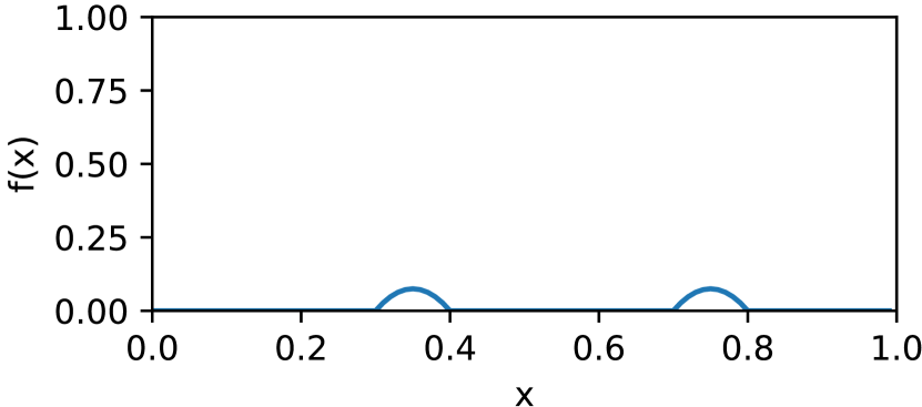
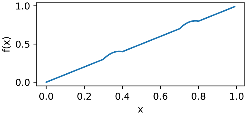
Figure 2: Original construction for nonparametric regression in 1-d (left), and our construction (right).

2.3 Nonparametric Regression using Noisy Ranking

In this section, we study the setting where the ordinal information is noisy. We focus here on the setting where as in equation (2) we obtain a ranking $\widehat{\pi}$ whose Kendall-Tau distance from the true ranking $\pi$ is at most $\nu n^{2}$. We show that the R² algorithm is quite robust to ranking errors and achieves an MSE of $\widetilde{O}(m^{-2/3}+\sqrt{\nu}+n^{-2s/d})$. We establish a complementary lower bound of $\widetilde{O}(m^{-2/3}+\nu^{2}+n^{-2s/d})$ in Section 2.3.2.

2.3.1 Upper Bounds for the R² Algorithm

We characterize the robustness of R² to ranking errors, i.e. when $\widehat{\pi}$ satisfies the condition in (2), in the following theorem:

Theorem 3

For constants $C_{1},C_{2}>0$, the MSE of the R² estimate $\widehat{f}$ is bounded by

$$\mathbb{E}[(\widehat{f}(X)-f(X))^{2}]\leq C_{1}\left(\log^{2}n\log m\left(m^{-2/3}+\sqrt{\nu}\right)\right)+C_{2}n^{-2s/d}.$$

Remarks: (1) Once again we observe that in the regime where sufficient ordinal information is available, i.e. when $n$ is large, the rate no longer has an exponential dependence on the dimension $d$.
(2) This result also shows that the R² algorithm is inherently robust to noise in the ranking, and the mean squared error degrades gracefully as a function of the noise parameter $\nu$. We investigate the optimality of the $\sqrt{\nu}$-dependence in the next section.

We now turn our attention to the proof of this result.

Proof Sketch  When using an estimated permutation $\widehat{\pi}$ the true function of interest $f$ is no longer an increasing (isotonic) function with respect to $\widehat{\pi}$, and this results in a model-misspecification bias. The core technical novelty of our proof is in relating the upper bound on the error in $\widehat{\pi}$ to an upper bound on this bias. Concretely, in the Appendix we show the following lemma:

Lemma 4

For any permutation $\widehat{\pi}$ satisfying the condition in (2)

$$\sum_{i=1}^{n}(f(X_{\pi^{-1}(i)})-f(X_{\widehat{\pi}^{-1}(i)}))^{2}\leq 8M^{2}\sqrt{2\nu}n.$$

Using this result we bound the minimal error of approximating an increasing sequence according to $\pi$ by an increasing sequence according to the estimated (and misspecified) ranking $\widehat{\pi}$. We denote this error on $m$ labeled points by $\Delta$, and using Lemma 4 we show that in expectation (over the random choice of the labeled set)

$$\mathbb{E}[\Delta]\leq 8M^{2}\sqrt{2\nu}m.$$

With this technical result in place we follow the same decomposition and subsequent steps before we arrive at the expression in equation (2.2.1). In this case, the first term for some constant $C>0$ is bounded as:

$$\mathbb{E}\Big{(}\sum_{k=1}^{m}\big{(}\widehat{f}(X_{t_{k}})-f(X_{t_{k}})\big{)}^{2}\Big{)}\leq 2\mathbb{E}[\Delta]+Cm^{1/3},$$

where the first term corresponds to the model-misspecification bias and the second corresponds to the usual isotonic regression rate. Putting these terms together in the decomposition in (2.2.1) we obtain the theorem.

 

In settings where $\nu$ is large R² can be led astray by the ordinal information, and a standard nonparametric regressor can achieve the (possibly faster) $O\big{(}m^{-\frac{2s}{2s+d}}\big{)}$ rate by ignoring the ordinal information. In this case, a simple and standard cross-validation procedure can combine the benefits of both methods: we estimate the regression function twice, once using R² and once using k nearest neighbors, and choose the regression function that performs better on a held-out validation set. The following theorem shows guarantees for this method and an upper bound for the minimax risk (1):

Theorem 5

Under the same assumptions as Theorem 3, there exists an estimator $\widehat{f}$ such that

$$\mathbb{E}[(\widehat{f}(X)-f(X))^{2}]=\widetilde{O}\left(m^{-2/3}+\min\{\sqrt{\nu},m^{-\frac{2s}{2s+d}}\}+n^{-2s/d}\right).$$

The main technical difficulty in analyzing the model-selection procedure we propose in this context is that a naïve analysis of the procedure, using classical tail bounds to control the deviation between the empirical risk and the population risk, results in an excess risk of $\widetilde{O}(1/\sqrt{m}).$ However, this rate would overwhelm the $\widetilde{O}(m^{-2/3})$ bound that arises from isotonic regression. We instead follow a more careful analysis outlined in the work of Barron (1991) which exploits properties of the squared-loss to obtain an excess risk bound of $\widetilde{O}(1/m).$ We provide a detailed proof in the Appendix for convenience and note that in our setting, the $y$ values are not assumed to be bounded and this necessitates some minor modifications to the original proof (Barron, 1991).

2.3.2 Lower bounds with Noisy Ordinal Data

In this section we turn our attention to lower bounds in the setting with noisy ordinal information. In particular, we construct a permutation $\widehat{\pi}$ such that for a pair $(X_{i},X_{j})$ of points randomly chosen from $\mathbb{P}_{\mathcal{X}}$:

$$\mathbb{P}[(\pi(i)-\pi(j))(\widehat{\pi}(i)-\widehat{\pi}(j))<0]\leq\nu.$$

We analyze the minimax risk of an estimator which has access to this noisy permutation $\widehat{\pi}$, in addition to the labeled and unlabeled sets (as in Section 2.2.2).

Theorem 6

There is a constant $C>0$ such that for any estimator $\widehat{f}$ taking input $X_{1},\ldots,X_{n},y_{1},\ldots,y_{m}$ and $\widehat{\pi}$,

$$\inf_{\widehat{f}}\sup_{f\in\mathcal{F}_{s,L}}\mathbb{E}\big{(}f(X)-\widehat{f}(X)\big{)}^{2}\geq C(m^{-\frac{2}{3}}+\min\{\nu^{2},m^{-\frac{2}{d+2}}\}+n^{-2s/d}).$$

Comparing this result with our result in Remark 3 following Theorem 3, our upper and lower bounds differ by the gap between $\sqrt{\nu}$ and $\nu^{2}$, in the case of Lipschitz functions ($s=1$).

Proof Sketch  We focus on the dependence on $\nu$, as the other parts are identical to Theorem 2. We construct a packing set of Lipschitz functions, and we subsequently construct a noisy comparison oracle $\widehat{\pi}$ which provides no additional information beyond the labeled samples. The construction of our packing set is inspired by the construction of standard lower bounds in nonparametric regression (see Figure 2), but we modify this construction to ensure that $\widehat{\pi}$ is uninformative. In the classical construction we divide $[0,1]^{d}$ into $u^{d}$ grid points, with $u=m^{1/(d+2)}$ and add a “bump” at a carefully chosen subset of the grid points. Here we instead divide $[0,t]^{d}$ into a grid with $u^{d}$ points, and add an increasing function along the first dimension, where $t$ is a parameter we choose in the sequel.

We now describe the ranking oracle which generates the permutation $\widehat{\pi}$: we simply rank sample points according to their first coordinate. This comparison oracle only makes an error when both $x,x^{\prime}$ lies in $[0,t]^{d}$, and both $x_{1},x_{1}^{\prime}$ lie in the same grid segment $[tk/u,t(k+1)/u]$ for some $k\in[u]$. So the Kendall-Tau error of the comparison oracle is $(t^{d})^{2}\times((1/u)^{2}\times u)=ut^{2d}$. We choose $t$ such that this value is less than $\nu$. Once again we complete the proof by lower bounding the cardinality of the packing-set for our stated choice of $t$, upper bounding the Kullback-Leibler divergence between the induced distributions and appealing to Fano’s inequality.  

2.4 Regression with Noisy Pairwise Comparisons

In this section we focus on the setting where the ordinal information is obtained in the form of noisy pairwise comparisons, following equation (3). We investigate a natural strategy of aggregating the pairwise comparisons to form a consensus ranking $\widehat{\pi}$ and then applying the R² algorithm with this estimated ranking. We build on results from theoretical computer science, where such aggregation algorithms are studied for their connections to sorting with noisy comparators. In particular, Braverman and Mossel (2009) study noisy sorting algorithms under the noise model described in (3) and establish the following result:

Theorem 7 (Braverman and Mossel (2009))

Let $\alpha>0$. There exists a polynomial-time algorithm using noisy pairwise comparisons between $n$ samples, that with probability $1-n^{-\alpha}$, returns a ranking $\widehat{\pi}$ such that for a constant $c(\alpha,\lambda)>0$ we have that:

$$\sum_{i,j\in[n]}\mathbb{I}[(\pi(i)-\pi(j))(\widehat{\pi}(i)-\widehat{\pi}(j))<0]\leq c(\alpha,\lambda)n.$$

Furthermore, if allowed a sequential (active) choice of comparisons, the algorithm queries at most $O(n\log n)$ pairs of samples.

Combining this result with our result on the robustness of R² we obtain an algorithm for nonparametric regression with access to noisy pairwise comparisons with the following guarantee on its performance:

Corollary 8

For constants $C_{1},C_{2}>0$, R² with $\widehat{\pi}$ estimated as described above produces an estimator $\widehat{f}$ with MSE

$$\mathbb{E}\big{(}\widehat{f}(X)-f(X)\big{)}^{2}\leq C_{1}m^{-2/3}\log^{2}n\log m+C_{2}\max\{n^{-2s/d},n^{-1/2}\log^{2}n\log m\}.$$

Remarks:

1. From a technical standpoint this result is an immediate corollary of Theorems 3 and 7, but the extension is important from a practical standpoint. The ranking error of $O(1/n)$ from the noisy sorting algorithm leads to an additional $\widetilde{O}(1/\sqrt{n})$ term in the MSE. This error is dominated by the $n^{-2s/d}$ term if $d\geq 4s$, and in this setting the result in Corollary 8 is also optimal up to log factors (following the lower bound in Section 2.2.2).
   

2. We also note that the analysis in Braverman and Mossel (2009) extends in a straightforward way to a setting where only a randomly chosen subset of the pairwise comparisons are obtained.

3 Linear Regression with Comparisons

In this section we investigate another popular setting for regression, that of fitting a linear predictor to data. We show that when we have enough comparisons, it is possible to estimate a linear function even when $m\ll d$, without making any sparsity or structural assumptions.

For linear regression we follow a different approach when compared to the nonparametric setting we have studied thus far. By exploiting the assumption of linearity, we see that each comparison now translates to a constraint on the parameters of the linear model, and as a consequence we are able to use comparisons to obtain a good initial estimate. However, the unknown linear regression parameters are not fully identified by comparison. For instance, we observe that the two regression vectors $w$ and $2\times w$ induce the same comparison results for any pairs $(X_{1},X_{2})$. This motivates using direct measurements to estimate a global scaling of the unknown regression parameters, i.e the norm of regression vector $w^{*}$. Essentially by using comparisons instead of direct measurements to estimate the weights, we convert the regression problem to a classification problem, and therefore can leverage existing algorithms and analyses from the passive/active classification literature.

We present our assumptions and notation for the linear setup in the next subsection. Then we give the algorithm along with its analysis in Section 3.2. We also present information-theoretic lower bounds on the minimax rate in Section 3.3.

3.1 Background and Problem Setup

Following some of the previous literature on estimating a linear classifier (Awasthi et al., 2014, 2016), we assume that the distribution $\mathbb{P}_{X}$ is isotropic and log-concave. In more detail, we assume that coordinates of $X$ are independent, centered around 0, have covariance $I_{d}$; and that the log of the density function of $X$ is concave. This assumption is satisfied by many standard distributions, for instance the uniform and Gaussian distributions (Lovász and Vempala, 2007). We let $B(v,r)$ denote the ball of radius $r$ around vector $v$. Our goal is to estimate a linear function $f(X)=\langle w^{*},\,X\rangle$, and for convenience we denote:

$$r^{*}=\|w^{*}\|_{2}~{}~{}~{}\text{and}~{}~{}~{}v^{*}=\frac{w^{*}}{\|w^{*}\|_{2}}.$$

Similar to the nonparametric case, we suppose that we have access to two kinds of supervision using labels and comparisons respectively. We represent these using the following two oracles:

• Label Oracle: We assume access to a label oracle $\mathcal{O}_{l}$, which takes a sample $X\in\mathbb{R}^{d}$ and outputs a label $y=\langle w^{*},\,X\rangle+\varepsilon$, with $\mathbb{E}[\varepsilon]=0$, $\text{Var}(\varepsilon)=\sigma^{2}$.

• Comparison Oracle: We also have access to a (potentially cheaper) comparison oracle $\mathcal{O}_{c}$. For each query, the oracle $\mathcal{O}_{c}$ receives a pair of samples $(X,X^{\prime})\sim\mathbb{P}_{X}\times\mathbb{P}_{X}$, and returns a random variable $Z\in\{-1,+1\}$, where $Z=1$ indicates that the oracle believes that $f(X)>f(X^{\prime})$, and $Z=-1$ otherwise. We assume that the oracle has agnostic noise $\nu$, i.e.:

  $$\mathbb{P}(Z\neq\text{sign}(\langle w^{*},\,X-X^{\prime}\rangle))\leq\nu.$$

  That is, for a randomly sampled triplet $(X,X^{\prime},Z)$ the oracle is wrong with probability at most $\nu$. Note that the error of the oracle for a particular example $(X,X^{\prime})=(x,x^{\prime})$ can be arbitrary.

Given a set of unlabeled instances $\mathcal{U}=\{X_{1},X_{2},\ldots\}$ drawn from $\mathbb{P}_{X}$, we aim to estimate $w^{*}$ by querying $\mathcal{O}_{l}$ and $\mathcal{O}_{c}$ with samples in $\mathcal{U}$, using a label and comparison budget of $m$ and $n$ respectively. Our algorithm can be either passive, active or semi-supervised; we denote the output of algorithm $\mathcal{A}$ by $\widehat{w}=\mathcal{A}(\mathcal{U},\mathcal{O}_{l},\mathcal{O}_{c})$. For an algorithm $\mathcal{A}$, we study the minimax risk (1), which in this case can be written as

$$\mathfrak{M}(m,n)=\inf_{\mathcal{A}}\sup_{w^{*}}\mathbb{E}\left[\langle w^{*}-\widehat{w},\,X\rangle^{2}\right].$$ (7)

Our algorithm relies on a linear classification algorithm $\mathcal{A}^{c}$, which we assume to be a proper classification algorithm (i.e. the output of $\mathcal{A}^{c}$ is a linear classifier which we denote by $\widehat{v}$). We let $\mathcal{A}^{c}(\mathcal{U},\mathcal{O},m)$ denote the output (linear) classifier of $\mathcal{A}^{c}$ when it uses the unlabeled data pool $\mathcal{U}$, the label oracle $\mathcal{O}$ and acquires $m$ labels. $\mathcal{A}^{c}$ can be either passive or active; in the former case the $m$ labels are randomly selected from $\mathcal{U}$, whereas in the latter case $\mathcal{A}^{c}$ decides which labels to query. We use $\varepsilon_{\mathcal{A}^{c}}(m,\delta)$ to denote (an upper bound on) the $0/1$ error of the algorithm $\mathcal{A}^{c}$ when using $m$ labels, with $1-\delta$ probability, i.e.:

$$\mathbb{P}[\text{err}(\mathcal{A}^{c}(\mathcal{U},m))\leq\varepsilon_{\mathcal{A}^{c}}(m,\delta)]\geq 1-\delta.$$

We note that by leveraging the log-concave assumption on $P_{X}$, it is straightforward to translate guarantees on the 0/1 error to corresponding guarantees on the $\ell_{2}$ error $\|\widehat{v}-v^{*}\|_{2}$.

We conclude this section by noting that the classical minimax rate for ordinary least squares (OLS) is of order $O(d/m)$, where $m$ is the number of label queries. This rate cannot be improved by active label queries (see for instance Chaudhuri et al. (2015)).

3.2 Algorithm and Analysis

Our algorithm, Comparison Linear Regression (CLR), is described in Algorithm 2. We first use the comparisons to construct a classification problem with samples $(X-X^{\prime})$ and oracle $\mathcal{O}_{c}$. Here we slightly overload the notation of $\mathcal{O}_{c}$ that $\mathcal{O}_{c}(X_{i}-X_{j})=\mathcal{O}_{c}(X_{i},X_{j})$. Given these samples we use an active linear classification algorithm to estimate a normalized weight vector $\widehat{v}$. After classification, we use the estimated $\widehat{v}$ along with actual label queries to estimate the norm of the weight vector $\widehat{r}$. Combining these results we obtain our final estimate $\widehat{w}=\widehat{r}\cdot\widehat{v}$.

Algorithm 2 Comparison Linear Regression (CLR)

0:  comparison budget $n$, label budget $m$, unlabeled data pool $\mathcal{U}$, algorithm $\mathcal{A}^{c}$

1:  Construct pairwise pool $\mathcal{U}^{\prime}=\{X_{1}-X_{2},X_{3}-X_{4},\ldots,X_{n-1}-X_{n}\}$

2:  Run $\mathcal{A}^{c}(\mathcal{U}^{\prime},\mathcal{O}_{c},n)$ and obtain a classifier with corresponding weight vector $\widehat{v}$

3:  Query random samples $\{(X_{i},y_{i})\}_{i=1}^{m}$

4:  Let $\displaystyle\widehat{r}=\frac{\sum_{i=1}^{m}\langle\widehat{v},\,X_{i}\rangle y_{i}}{\sum_{i=1}^{m}\langle\widehat{v},\,X_{i}\rangle^{2}}$.

4:  $\displaystyle\widehat{w}=\widehat{r}\cdot\widehat{v}$.

We have the following main result which relates the error of $\widehat{w}$ to the error of the classification algorithm $\mathcal{A}^{c}$.

Theorem 9

There exists some constants $C,M$ such that if $m>M$, the MSE of Algorithm 2 satisfies

$$\mathbb{E}[\langle w^{*}-\widehat{w},\,X\rangle^{2}]\leq\widehat{O}\left(\frac{1}{m}+\log^{2}m\cdot\varepsilon_{\mathcal{A}^{c}}\left(n,\frac{1}{m}\right)+\nu^{2}\right).$$

We defer a detailed proof to the Appendix and provide a concise proof sketch here.

Proof Sketch

We recall that, by leveraging properties of isotropic log-concave distributions, we can obtain an estimator $\widehat{v}$ such that $\|\widehat{v}-v^{*}\|_{2}\leq\varepsilon=O\left(\varepsilon_{\mathcal{A}^{c}}(n,\delta)\right)$. Now let $T_{i}=\langle\widehat{v},\,X_{i}\rangle$, and we have

$$\widehat{r}=\frac{\sum_{i=1}^{m}T_{i}y_{i}}{\sum_{i=1}^{m}T_{i}^{2}}=r^{*}+\frac{\sum_{i=1}^{m}T_{i}r^{*}\langle v^{*}-\widehat{v},\,X_{i}\rangle+\varepsilon_{i}}{\sum_{i=1}^{m}T_{i}^{2}}.$$

And thus

$$\langle w^{*},\,X\rangle-\langle\widehat{w},\,X\rangle=r^{*}\langle v^{*}-\widehat{v},\,X\rangle-\frac{\sum_{i=1}^{m}T_{i}r^{*}\langle v^{*}-\widehat{v},\,X_{i}\rangle}{\sum_{i=1}^{m}T_{i}^{2}}\langle\widehat{v},\,X\rangle+\frac{\sum_{i=1}^{m}T_{i}\varepsilon_{i}}{\sum_{i=1}^{m}T_{i}^{2}}\langle\widehat{v},\,X\rangle.$$

The first term can be bounded using $\|\widehat{v}-v^{*}\|_{2}\leq\varepsilon$; for the latter two terms, using Hoeffding bounds we show that $\sum_{i=1}^{m}T_{i}^{2}=O(m)$. Then by decomposing the sums in the latter two terms, we can bound the MSE.  

Leveraging this result we can now use existing results to derive concrete corollaries for particular instantiations of the classification algorithm $\mathcal{A}^{c}$. For example, when $\nu=0$ and we use passive learning, standard VC theory shows that the empirical risk minimizer has error $\varepsilon_{\text{ERM}}=O(d\log(1/\delta)/n)$. This leads to the following corollary:

Corollary 10

Suppose that $\nu=0$, and that we use the passive ERM classifier as $\mathcal{A}^{c}$ in Algorithm 2, then the output $\widehat{w}$ has MSE bounded as:

$$\mathbb{E}[\langle w^{*}-\widehat{w},\,X\rangle^{2}]\leq\widehat{O}\left(\frac{1}{m}+\frac{d\log^{3}m}{n}\right).$$

When $\nu>0$, we can use other existing algorithms for either the passive/active case. We give a summary of existing results in Table 1, and note that (as above) each of these results can be translated in a straightforward way to a guarantee on the MSE when combining direct and comparison queries. We also note that previous results using isotropic log-concave distribution can be directly exploited in our setting since $X-X^{\prime}$ follows isotropic log-concave distribution if $X$ does (Lovász and Vempala, 2007). Each of these results provide upper bounds on minimax risk (7) under certain restrictions.

Table 1: Summary of existing results for passive/active classification for isotropic log-concave $X$ distributions. $C$ denotes some fixed constant; $\varepsilon=\varepsilon_{\mathcal{A}^{c}}(m,\delta)$. The work of Yan and Zhang (2017) additionally requires that $X-X^{\prime}$ follow a uniform distribution.

Algorithm	Oracle	Requirement	Rate of $\varepsilon$	Efficient?
ERM (Hanneke, 2009)	Passive	None	$\widetilde{O}\left(d\sqrt{\frac{1}{m}}\right)$	No
		$\nu=O(\varepsilon)$	$\widetilde{O}\left(\frac{d}{m}\right)$
Awasthi et al. (2016)	Passive	$\nu=O(\varepsilon)$	$\widetilde{O}\left(\left(\frac{d}{m}\right)^{1/3}\right)$	Yes
Awasthi et al. (2014)	Active	$\nu=O(\varepsilon)$	$\exp\left(-\frac{Cm}{d+\log(m/\delta)}\right)$	Yes
Yan and Zhang (2017)	Passive	$\nu=O\left(\frac{\varepsilon}{\log d+\log\log\frac{1}{\varepsilon}}\right)$	$\widetilde{O}\left(\frac{d}{m}\right)$	Yes
	Active		$\exp\left(-\frac{Cm}{d+\log(m/\delta)}\right)$

3.3 Lower Bounds

Now we turn to information-theoretic lower bounds on the minimax risk (1). We consider any active estimator $\widehat{w}$ with access to the two oracles $\mathcal{O}_{c},\mathcal{O}_{l}$, using $n$ comparisons and $m$ labels. In this section, we show that the $1/m$ rate in Theorem 9 is optimal; we also show a lower bound in the active setting on the total number of queries in the appendix.

Theorem 11

Suppose that $X$ is uniform on $[-1,1]^{d}$, and $\varepsilon\sim\mathcal{N}(0,1)$. Then, for any (active) estimator $\widehat{w}$ with access to both label and comparison oracles, there is a universal constant $c>0$ such that,

$$\inf_{\widehat{w}}\sup_{w^{*}}\mathbb{E}\left[\langle w^{*}-\widehat{w},\,X\rangle^{2}\right]\geq\frac{c}{m}.$$

Theorem 11 shows that the $O(1/m)$ term in Theorem 9 is necessary. The proof uses classical information-theoretic techniques (Le Cam’s method) applied to two increasing functions with $d=1$, and is included in Appendix B.7.

We note that we cannot establish lower bounds that depend solely on number of comparisons $n$, since we can of course achieve $O(d/m)$ MSE without using any comparisons. Consequently, we show a lower bound on the total number of queries in Appendix B.8. This bound shows that when using the algorithm in the paper of Awasthi et al. (2014) as $\mathcal{A}^{c}$ in CLR, the total number of queries is optimal up to log factors.

4 Experiments

To verify our theoretical results and test our algorithms in practice, we perform three sets of experiments. First, we use simulated data, where the noise in the labels and ranking can be controlled separately. Second, we consider an application of predicting people’s ages from photographs, where we synthesize comparisons from data on people’s apparent ages (as opposed to their true biological ages). Finally, we crowdsource data using Amazon’s Mechanical Turk to obtain comparisons and direct measurements for the task of estimating rental property asking prices. We then evaluate various algorithms for predicting rental property prices, both in terms of their accuracy, as well as in terms of their time cost.

Baselines. In the nonparametric setting, we compare R² with $k$-NN algorithms in all experiments. We choose $k$-NN methods because they are near-optimal theoretically for Lipschitz functions, and are widely used in practice. Also, the R² method is a nonparametric method built on a nearest neighbor regressor. It may be possible to use the ranking-regression method in conjunction with other nonparametric regressors but we leave this for future work. We choose from a range of different constant values of $k$ in our experiments.

In the linear regression setting, for our CLR algorithm, we consider both a passive and an active setting for comparison queries. For the passive comparison query setting, we simply use a Support Vector Machine (SVM) as $\mathcal{A}$ in Algorithm 2. For the active comparison query setting, we use an algorithm minimizing hinge loss as described in Awasthi et al. (2014). We compare CLR to the LASSO and to Linear Support Vector Regression (LinearSVR), where the relevant hyperparameters are chosen based on validation set performance. We choose LASSO and LinearSVR as they are the most prevalent linear regression methods. Unless otherwise noted, we repeat each experiment 20 times and report the average MSE.

Cost Ratio. Our algorithms aim at reducing the overall cost of estimating a regression function when comparisons can be more easily available than direct labels. In practice, the cost of obtaining comparisons can vary greatly depending on the task, and we consider two practical setups:

1. In many applications, both direct labels and comparisons can be obtained, but labels cost more than comparisons. Our price estimation task corresponds to this case. The cost, in this case, depends on the ratio between the cost of comparisons and labels. We suppose that comparisons cost 1, and that labels cost $c$ for some constant $c>1$ and that we have a total budget of $C$. We call $c$ the cost ratio. Minimizing the risk of our algorithms requires minimizing $\mathfrak{M}(m,n;\eta)$ as defined in (1) subject to $cm+n\leq C$; for most cases, we need a small $m$ and large $n$. In experiments with a finite cost ratio, we fix the number of direct measurements to be a small constant $m$ and vary the number of comparisons that we use.

2. Direct labels might be substantially harder to acquire because of privacy issues or because of inherent restrictions in the data collection process, whereas comparisons are easier to obtain. Our age prediction task corresponds to this case, where it is conceivable that only some of the biological ages are available due to privacy issues. In this setting, the cost is dominated by the cost of the direct labels and we measure the cost of estimation by the number of labeled samples used.

4.1 Modifications to Our Algorithms

While R² and CLR are near optimal from a theoretical standpoint, we adopt the following techniques to improve their empirical performance:

R² with $k$-NN. Our analysis considers the case when we use 1-NN after isotonic regression. However, we empirically find that using more than 1 nearest neighbor can also improve the performance. So in our experiments, we use $k$-NN in the final step of R², where $k$ is a small fixed constant. We note in passing that our theoretical results remain valid in this slightly more general setting.

R² with comparisons. When R² uses passively collected comparisons, we would need $O(n^{2})$ pairs to have a ranking with $O(1/n)$ error in the Kendall-Tau metric if we use the algorithm from Braverman and Mossel (2009). We instead choose to take advantage of the feature space structure when we use R² with comparisons. Specifically, we build a nonparametric rankSVM (Joachims, 2002) to score each sample using pairwise comparisons. We then rank samples according to their scores given by the rankSVM. We discuss another potential method, which uses nearest neighbors based on Borda counts, in Appendix A.

CLR with feature augmentation. Using the directly labeled data only to estimate the norm of the weights corresponds to using linear regression with the direct labels with a single feature $\langle\widehat{v},\,x\rangle$ from Algorithm 2. Empirically, we find that using all the features together with the estimated $\langle\widehat{v},\,x\rangle$ results in better performance. Concretely, we use a linear SVR with input features $(x;\langle\widehat{v},\,x\rangle)$, and use the output as our prediction.

4.2 Simulated Data

We generate different synthetic datasets for nonparametric and linear regression settings in order to verify our theory.

4.2.1 Simulated Data for R²

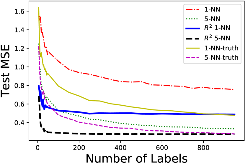
(a) Perfect ranking

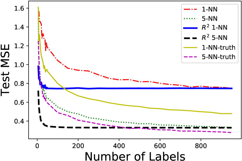
(b) Noisy ranking

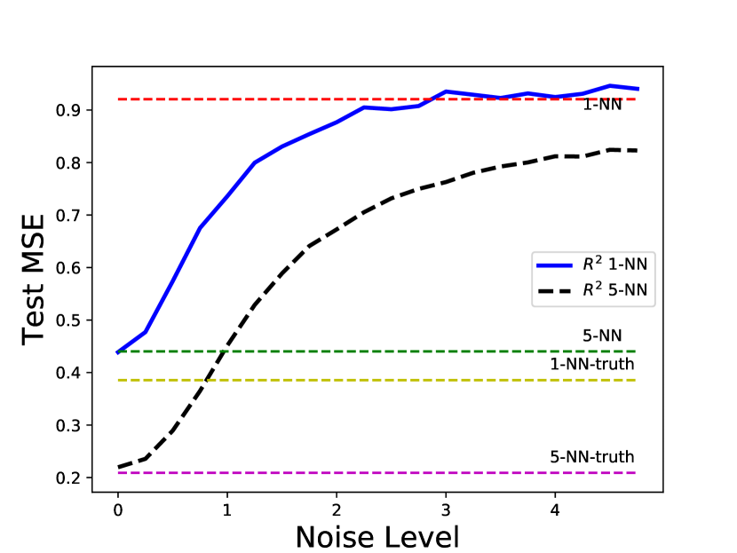
(c) Effect of ranking noise, $m=100$

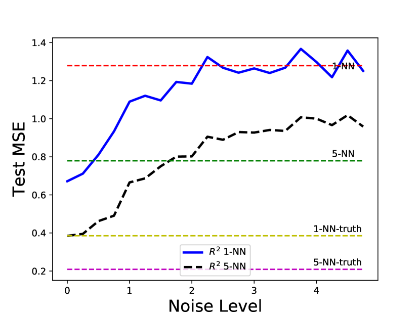
(d) Effect of ranking noise, $m=10$

Figure 3: Experiments on simulated data for R². 1-NN and 5-NN represent algorithms using noisy label data only; R² 1-NN and R² 5-NN use noisy labels as well as rankings; 1-NN-truth and 5-NN-truth use perfect label data only.

Data Generation. We generate simulated data following Härdle et al. (2012). We take $d=8$, and sample $X$ uniformly random from $[0,1]^{d}$. Our target function is $f(x)=\sum_{i=1}^{d}f^{(i\text{ mod }4)}(x_{i})$, where $x_{i}$ is $x$’s $i$-th dimension, and

$$f^{(1)}(x)=px-1/2,~{}~{}~{}~{} f^{(2)}(x)=px^{3}-1/3,$$

$$f^{(3)}(x)=-2\sin(-px),~{}~{}~{}~{}~{} f^{(4)}(x)=e^{-px}+e^{-1}-1$$

with $p$ sampled uniformly at random in $[0,10]$. We generate a training and a test set each of size $n=1000$ samples respectively. We rescale $f$ so that it has 0 mean and unit variance over the training set. This makes it easy to control the noise that we add relative to the function value. For training data, we generate the labels as $y_{i}=f(X_{i})+\varepsilon$ where $\varepsilon\sim\mathcal{N}(0,0.5^{2})$, for the training data $\{X_{1},\ldots,X_{n}\}$. At test time, we compute the MSE $\frac{1}{n}\sum_{i=1}^{n}(f(X^{\text{test}}_{i})-\widehat{f}(X^{\text{test}}_{i}))^{2}$ for the test data $\{X^{\text{test}}_{1},\ldots,X^{\text{test}}_{n}\}$.

Setup and Baselines. We test R² with either 1-NN or 5-NN for our simulated data, denoted as R² 1-NN and R² 5-NN respectively. We compare them with the following baselines: i) 1-NN and 5-NN using noisy labels $(X,y)$ only. Since R² uses ordinal data in addition to labels, it should have lower MSE than 1-NN and 5-NN. ii) 1-NN and 5-NN using perfect labels $(X,f(X))$. Since these algorithms use perfect labels, when all sample points are labeled they serve as a benchmark for our algorithms.

R² with rankings. Our first set of experiments suppose that R² has access to the ranking over all 1000 training samples, while the $k$-NN baseline algorithms only have access to the labeled samples. We measure the cost as the number of labels in this case. Figure 3(a) compares R² with baselines when the ranking is perfect. R² 1-NN and R² 5-NN exhibited better performance than their counterparts using only labels, whether using noisy or perfect labels; in fact, we find that R² 1-NN and R² 5-NN perform nearly as well as 1-NN or 5-NN using all 1000 perfect labels, while only requiring around 50 labeled samples.

In Figure 3(b), R² uses an input ranking obtained from noisy labels $\{y_{1},...,y_{n}\}$. In this case, the noise in the ranking is dependent on the label noise, since the ranking is directly derived from the noisy labels. This makes the obtained labels consistent with the ranking, and thus eliminates the need for isotonic regression in Algorithm 1. Nevertheless, we find that the ranking still provides useful information for the unlabeled samples. In this setting, R² outperformed its 1-NN and 5-NN counterparts using noisy labels. However, R² was outperformed by algorithms using perfect labels when $n=m$. As expected, R² and $k$-NN with noisy labels achieved identical MSE when $n=m$, as ranking noise is derived from noise in labels.

We consider the effect of independent ranking noise in Figure 3(c). We fixed the number of labeled/ranked samples to 100/1000 and varied the noise level of ranking. For a noise level of $\sigma$, the ranking is generated from

$$y^{\prime}=f(X)+\varepsilon^{\prime}$$ (8)

where $\varepsilon^{\prime}\sim\mathcal{N}(0,\sigma^{2})$. We also plot the performance of 1-NN and 5-NN using 100 noisy labels and 1,000 perfect labels for comparison. We varied $\sigma$ from 0 to 5 and plotted the MSE. We repeat these experiments 50 times.

For both R² 1-NN and 5-NN – despite the fact that they use noisy labels – their performance is close to the NN methods using noiseless labels. As $\sigma^{\prime}$ increases, both methods start to deteriorate, with R² 5-NN hitting the naive 5-NN method at around $\sigma^{\prime}=1$ and R² 1-NN at around $\sigma^{\prime}=2.5$. This shows that R² is robust to ranking noise of comparable magnitude to the label noise. We show in Figure 3(d) the curve when we use 10 labels and 1000 ranked samples, where a larger amount of ranking noise can be tolerated.

R² with comparisons. We also investigate the performance of R² when we have pairwise comparisons instead of a total ranking. We train a rankSVM with an RBF kernel with a bandwidth of 1, i.e. $k(x,x^{\prime})=\exp(-\|x-x^{\prime}\|_{2}^{2})$, as described in Section 4.1. Our rankSVM has a ranking error of $\nu=11.8\%$ on the training set and $\nu=13.8\%$ on the validation set. For simplicity, we only compare with 5-NN here since it gives best performance amongst the label-only algorithms. The results are depicted in Figure 4. When comparisons are perfect, we first investigate the effect of the cost ratio in Figure 4(a). We fixed the budget to equal to $C=500c$ (i.e., we would have 500 labels available if we only used labels), and each curve corresponds to a value of $m\in\{50,100,200\}$ and a varied $n$ such that the total cost is $C=500c$. We can see for almost all choices of $m$ and cost ratio, R² provides a performance boost. In Figure 4(b) we fix $c=5$, and vary the total budget $C$ from 500 to 4,000. We find that R² outperforms the label-only algorithms in most setups.

In Figures 4(c) and 4(d), we consider the same setup of experiments, but with comparisons generated from (8), where $\varepsilon^{\prime}\sim\mathcal{N}(0,0.5^{2})$. Note that here the noise $\varepsilon^{\prime}$ is of the same magnitude but independent from the label noise. Although R² gave a less significant performance boost in this case, it still outperformed label-only algorithms when $c\geq 2$.

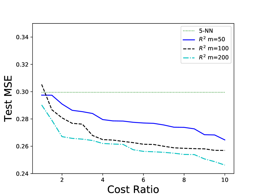
(a) Perfect comparisons, $C=500c$

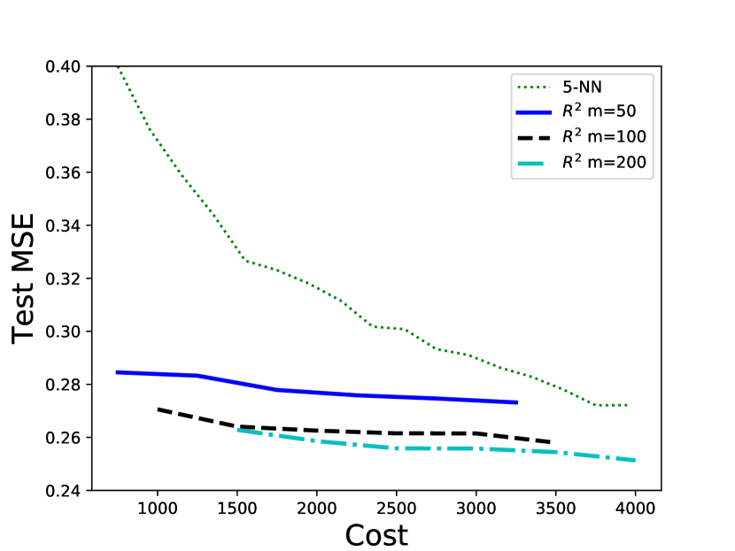
(b) Perfect comparisons, $c=5$

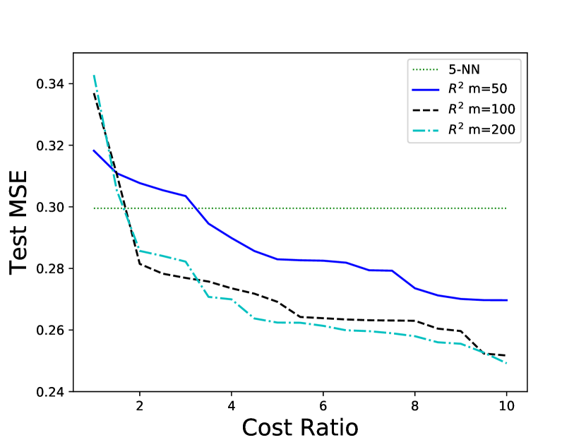
(c) Noisy comparisons, $C=500c$

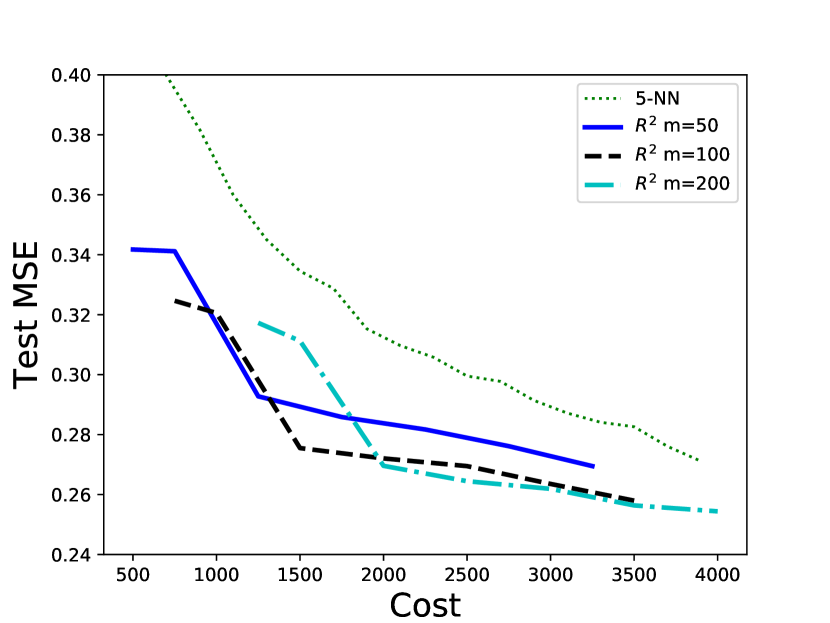
(d) Noisy comparisons, $c=5$

Figure 4: Experimental results on synthetic dataset for R² with comparisons. Each curve corresponds to a fixed $m$, and we vary $n$ as the cost ratios or total budget change. Note that curves start at different locations because of different $m$ values.

4.2.2 Simulated Data for CLR

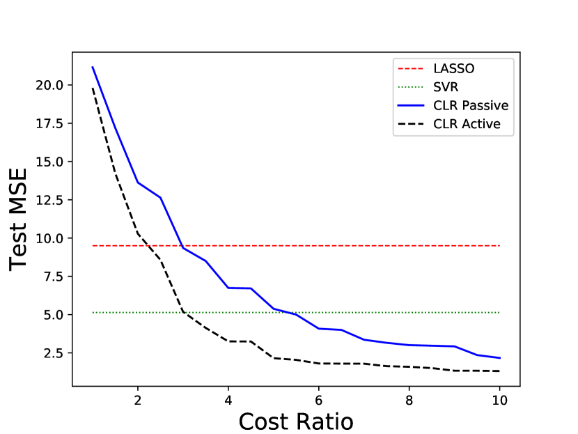
(a) Varying cost ratio $c$ with $C=50c$

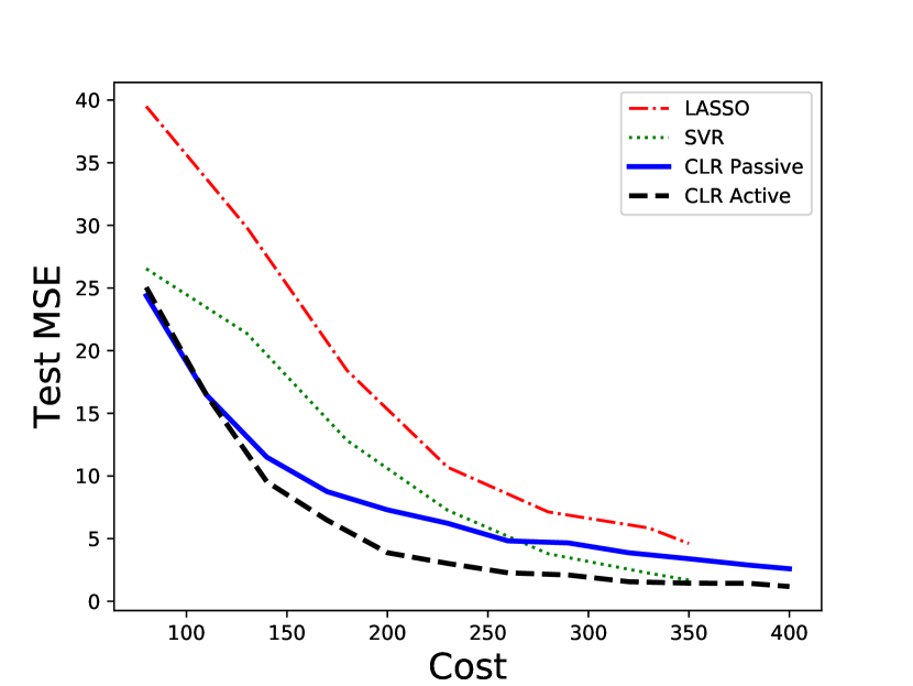
(b) Varying budget $C$ with $c=5$

Figure 5: Experimental results on synthetic dataset for CLR.

For CLR we only consider the case with a cost ratio, because we find that a small number of comparisons already suffice to obtain a low error. We set $d=50$ and generate both $X$ and $w^{*}$ from the standard normal distribution $\mathcal{N}(0,I_{d})$. We generate noisy labels with distribution $\varepsilon\sim\mathcal{N}(0,0.5^{2})$. The comparison oracle generates response using the same noise model: $Z=\text{sign}((\langle w^{*},\,x_{1}\rangle+\varepsilon_{1})-(\langle w^{*},\,x_{2}\rangle-\varepsilon_{2}))$ for input $(x_{1},x_{2})$, with $\varepsilon_{1},\varepsilon_{2}\sim\mathcal{N}(0,0.5^{2})$ independent of the label noise.

Model performances are compared in Figure 5. We first investigate the effect of cost ratio in Figure 5(a), where we fixed the budget to $C=50c$, i.e. if we only used labels we would have a budget of 50 labels. The passive comparison query version of CLR requires roughly $c>5$ to outperform baselines, and the active comparison query version requires $c>3$. We also experiment with a fixed cost ratio $c=5$ and varying budget $C$ in Figure 5(b). The active version outperformed all baselines in most scenarios, whereas the passive version gave a performance boost when the budget was less than 250 (i.e. number of labels is restricted to less than 250 in label only setting). We note that the active and passive versions of CLR only differ in their collection of comparisons; both algorithms (along with the baselines) are given a random set of labeled samples, making it a fair competition.

4.3 Predicting Ages from Photographs

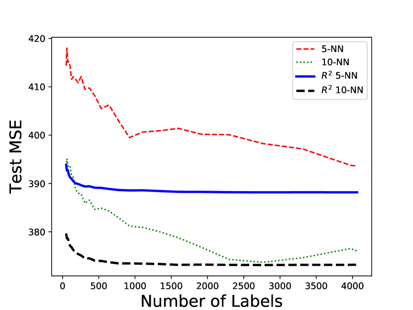
(a) R²

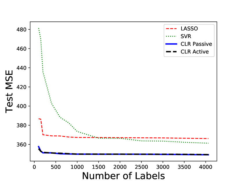
(b) Linear Regression

Figure 6: Experimental results on age prediction.

To further validate R² in practice, we consider the task of estimating people’s ages from photographs. We use the APPA-REAL dataset (Agustsson et al., 2017), which contains 7,591 images, and each image is associated with a biological age and an apparent age. The biological age is the person’s actual age, whereas the apparent ages are collected by asking crowdsourced workers to estimate their apparent ages. Estimates from (on average 38 different) labelers are averaged to obtain the apparent age. APPA-REAL also provides the standard deviation of the apparent age estimates. The images are divided into 4,063 train, 1,488 validation and 1,962 test samples, and we choose the best hyperparameters using the validation samples.

Task. We consider the task of predicting biological age. Direct labels come from biological age, whereas the ranking is based on apparent ages. This is motivated by the collection process of many modern datasets: for example, we may have the truthful biological age only for a fraction of samples, but wish to collect more through crowdsourcing. In crowdsourcing, people give comparisons based on apparent age instead of biological age. As a consequence, in our experiments we assume additional access to a ranking that comes from the apparent ages. Since collecting crowdsourced data can be much easier than collecting the real biological ages, as discussed earlier, we define the cost as the number of direct labels used in this experiment.

Features and Models. We extract a 128-dimensional feature vector for each image using the last layer of FaceNet (Schroff et al., 2015). We rescale the features so that every $X\in[0,1]^{d}$ for R², or we centralize the feature to have zero mean and unit variance for CLR. We use 5-NN and 10-NN to compare with R² in this experiment. Utilizing extra ordinal information, R² has additional access to the ranking of apparent ages; since CLR does not use a ranking directly we provide it access to 4,063 comparisons (the same size as the training set) based on apparent ages.

Our results are depicted in Figure 6. The 10-NN version of R² gave the best overall performance amongst nonparametric methods. R² 5-NN and R² 10-NN both outperformed other algorithms when the number of labeled samples was less than 500. Interestingly, we observe that there is a gap between R² and its nearest neighbor counterparts even when $n=m$, i.e. the ordinal information continues to be useful even when all samples are labeled; this might be because the biological ages are “noisy” in the sense that they are also determined by factors not present in image (e.g., lifestyle). Similarly, for linear regression methods, our method also gets the lowest overall error for any budget of direct labels. In this case, we notice that active comparisons only have a small advantage over passive comparisons, since the comparison classifiers both converge with a sufficient number of comparisons.

4.4 Estimating AirBnB Listing Prices

In our third set of experiments, we consider the cost of both comparisons and direct labels. We use data of AirBnB listings and ask Amazon Mechanical Turk (AMT) workers to estimate their price. To measure the cost, we collect not only the labels and comparisons but also the time taken to answer the question. We use the time as an estimate of the cost.

Data Collection. Our data comes from Kaggle and contains information about AirBnB postings in Seattle. We use 357 listings as the training set and 93 as the test set. We additionally pick 50 listings from the training set as validation data to select hyperparameters. We use the following features for our experiments:

(1) Host response rate,	(2) Host acceptance rate,	(3) Host listings count,
(4) Number of reviews per month,	(5) Number of bathrooms,	(6) Number of bedrooms,
(7) Number of beds,	(8) Number of reviews,	(9) Review scores rating,
(10) Number of people the house accommodates.

Each worker from AMT is asked to do either of the following two tasks: i) given the description of an AirBnB listing, estimate the per-night price on a regular day in 2018; ii) given the description of two AirBnB listings, select the listing that has a higher price. We collect 5 direct labels for each data point in the training set and 9 labels for each data point in the test set. For comparisons, we randomly draw 1,841 pairs from the training set and ask 2 workers to compare their prices.

Tasks. We consider two tasks, motivated by real-world applications.

1. In the first task, the goal is to predict the real listing price. This is motivated by the case where collecting the real price might be difficult to obtain or involves privacy issues. We assume that our training data, including both labels and comparisons, comes from AMT workers.

2. In the second task, the goal is to predict the user-estimated price. This can be of particular interest to AirBnB company and house-owners, for deciding the best price of the listing. We do not use the real prices in this case; we use the average of 10 worker estimated prices for each listing in the test set as the ground truth label, and the training data also comes from our AMT results.

Raw Data Analysis. Before we proceed to the regression task, we analyze the workers’ performance for both tasks based on raw data in Table 2. Our first goal is to compare a pairwise comparison to an induced comparison, where the induced comparison is obtained by making two consecutive direct label queries and subtracting them. Similar to Shah et al. (2016a), we observe that comparisons are more accurate than the induced comparisons.

We first convert labels into pairwise comparisons by comparing individual direct labels: namely, for each obtained labeled sample pair $(x_{1},y_{1}),(x_{2},y_{2})$ where $y_{1},y_{2}$ are the raw labels from workers, we create a pairwise comparison that corresponds to comparing $(x_{1},x_{2})$ with label being sign$(y_{1}-y_{2})$. We then compute the error rate of raw and label-induced comparisons for both Task 1 and 2. For Task 1, we directly compute the error rate w.r.t. the true listing price. For Task 2, we do not have the ground truth user prices; we instead follow the approach of Shah et al. (2016a) to compute the fraction of disagreement between comparisons. Namely, in either the raw or label-induced setting, for every pair of samples $(x_{i},x_{j})$ we compute the majority of labels $z_{ij}$ based on all comparisons on $(x_{i},x_{j})$. The disagreement on $(x_{i},x_{j})$ is computed as the fraction of comparisons that disagrees with $z_{ij}$, and we compute the overall disagreement by averaging over all possible $(x_{i},x_{j})$ pairs.

If an ordinal query is equivalent to two consecutive direct queries and subtracting the labels, we would expect a similar accuracy/disagreement for the two kinds of comparisons. However our results in Table 2 show that this is not the case: direct comparison queries have better accuracy for Task 1, as well as a lower disagreement within collected labels. This shows that a comparison query cannot be replaced by two consecutive direct queries. We do not observe a large difference in the average time to complete a query in Table 2; however the utility of comparisons in predicting price can be higher since they yield information about two labels. Further analysis of the raw data is given in Appendix A.

Performance	Comparisons	Labels
Task 1 Error	31.3%	41.3%
Task 2 Disagreement	16.4%	29.5%
Average Time	64s	63s

Table 2: Performance of comparisons versus labels for both tasks.

Results. We plot the experimental results in Figure 7. For nonparametric regression, R² had a significant performance boost over the best nearest neighbor regressor under the same total worker time, especially for Task 1. For Task 2, we observe a smaller improvement, but R² is still better than pure NN methods for all total time costs.

For linear regression, we find that the performance of CLR varies greatly with $m$ (number of labels), whereas its performance does not vary as significantly with the number of comparisons. In fact, the errors of both CLR passive and active already plateau with a mere 50 comparisons, since the dimension of data is small ($d=10$). So deviating from our previous experiments, in this setting, we vary the number of labels in Figure 7(c) and 7(d). As in the nonparametric case, CLR also outperforms the baselines in both tasks. For Task 1, the active and passive versions of CLR perform similarly, whereas active queries lead to a moderate performance boost on Task 2. This is probably because the error on Task 2 is much lower than that on Task 1 (see Table 2), and active learning typically has an advantage over passive learning when the noise is not too high.

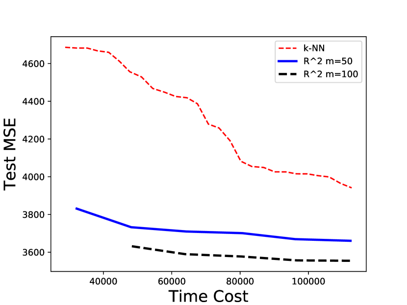
(a) Nonparametric, Task 1

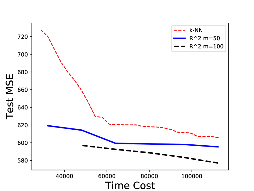
(b) Nonparametric, Task 2

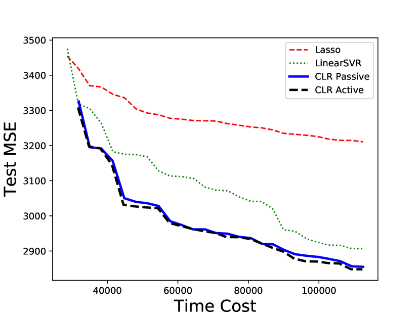
(c) Linear, Task 1

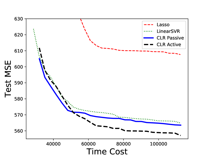
(d) Linear, Task 2

Figure 7: Results for AirBnB price estimation. In (a)(b), each curve has a fixed $m$ with varied $n$; for (c)(d), each curve uses only 50 comparisons with a varied number of labels. For Figure (d), LASSO performs much worse than a LinearSVR and we only show part of the curve.

5 Discussion

We design (near) minimax-optimal algorithms for nonparametric and linear regression using additional ordinal information. In settings where large amounts of ordinal information are available, we find that limited direct supervision suffices to obtain accurate estimates. We provide complementary minimax lower bounds, and illustrate our proposed algorithms on real and simulated datasets. Since ordinal information is typically easier to obtain than direct labels, one might expect in these favorable settings the R² algorithm to have lower effective cost than an algorithm based purely on direct supervision.

Several directions exist for future work. On nonparametric regression side, it remains to extend our results to the case where the Hölder exponent $s>1$. In this setting the optimal rate $O\left(m^{-\frac{-2s}{2s+d}}\right)$ can be faster than the convergence rate of isotonic regression, which can make our algorithm sub-optimal. It is also important to address the setting where both direct and ordinal supervision are actively acquired. For linear regression, an open problem is to consider the bounded noise model for comparisons. Our results can be easily extended to the bounded noise case using the algorithm in Hanneke (2009), however that algorithm is computationally inefficient. The best efficient active learning algorithm in this bounded noise setting (Awasthi et al., 2016) requires $m\geq O\left(d^{O(\frac{1}{(1-2\lambda)^{4}})}\right)$ comparisons, and a large gap remains between what can be achieved in the presence and absence of computational constraints.

Motivated by practical applications in crowdsourcing, we list some further extensions to our results:

Partial orders: In this paper, we focus on ordinal information either in the form of a total ranking or pairwise comparisons. In practice, ordinal information might come in the form of partial orders, where we have several subsets of unlabeled data ranked, but the relation between these subsets is unknown. A straightforward extension of our results in the nonparametric case leads to the following result: if we have $k$ (partial) orderings, each with $n_{1},\ldots,n_{k}$ samples, and $m_{1},\ldots,m_{k}$ samples in each ordering are labeled, we can show an upper bound on the MSE of $m_{1}^{-2/3}+\cdots+m_{k}^{-2/3}+(n_{1}+\cdots+n_{k})^{-2s/d}$. It would be interesting to study the optimal rate, as well as to consider other smaller partial orders.

Other models for ordinal information: Beyond the bounded noise model for comparison, we can consider other pairwise comparison models, like Plackett-Luce (Plackett, 1975; Luce, 2005) and Thurstone (Thurstone, 1927). These parametric models can be quite restrictive and can lead to unnatural results that we can recover the function values even without querying any direct labels (see for example Shah et al. (2016a)). One might also consider pairwise comparisons with Tsybakov-like noise Tsybakov (2004) which have been studied in the classification setting Xu et al. (2017); the main obstacle here is the lack of computationally-efficient algorithms that aggregate pairwise comparisons into a complete ranking under this noise model.

Other classes of functions: Several recent papers (Chatterjee et al., 2015; Bellec and Tsybakov, 2015; Bellec, 2018; Han et al., 2017) demonstrate the adaptivity (to “complexity” of the unknown parameter) of the MLE in shape-constrained problems. Understanding precise assumptions on the underlying smooth function which induces a low-complexity isotonic regression problem is interesting future work.

A Additional Experimental Results

Relation between true and user estimated price. Figure 8 shows a scatter plot of the true listing prices of AirBnB data with respect to the user estimated prices. Although the true prices is linearly correlated with the user prices (with $p$-value $6e-20$), the user price is still very different from true price even if we take the average of 5 labelers. The average of all listings’ true price is higher than the average of all user prices by 25 dollars, partially explaining the much higher error when we use user prices to estimate true prices.

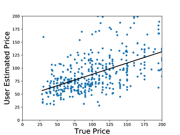
Figure 8: Scatter plot of true prices w.r.t average user estimated prices, along with the ordinary least square result. We only show prices smaller than 200 to make the relation clearer.

An alternative to using RankSVM. As an alternative to training RankSVM, we can also use nearest neighbors on Borda counts to take into account the structure of feature space: for each sample $x$, we use the score $s(x)=\frac{1}{k}\sum_{x^{\prime}\in k\text{-NN}(x)}\text{Borda}(x^{\prime})$, where $k$-NN$(x)$ is the $k$-th nearest neighbor of $x$ in the feature space, including $x$ itself. The scores are then used to produce a ranking. When $c$ is large, this method does provide an improvement over the label-only baselines, but generally does not perform as well as our rankSVM method. The results when cost ratio $c=10$ and comparisons are perfect are depicted in Figure 9. We use $k=25$ for deciding the nearest neighbors for Borda counts, and 5-NN as the final prediction step. While using R² with Borda counts do provide a gain over label-only methods, the improvement is less prominent than using rankSVM.

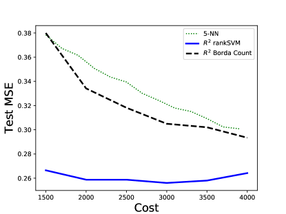
Figure 9: Experimental results on synthetic dataset for R² with comparisons, using nearest neighbor with Borda counts. Both R² algorithms uses 5-NN as the final prediction step.

For estimating AirBnB price the results are shown in Figure 10. For task 1, NN of Borda counts introduces an improvement similar to (or less than) RankSVM, but for task 2 it is worse than nearest neighbors. We note that for task 1, the best number of nearest neighbors of Borda counts is 50, whereas for task 2 it is 5 (close to raw Borda counts). We suspect this is due to the larger noise in estimating true price, however a close examination for this observation remains as future work.

(a) Task 1

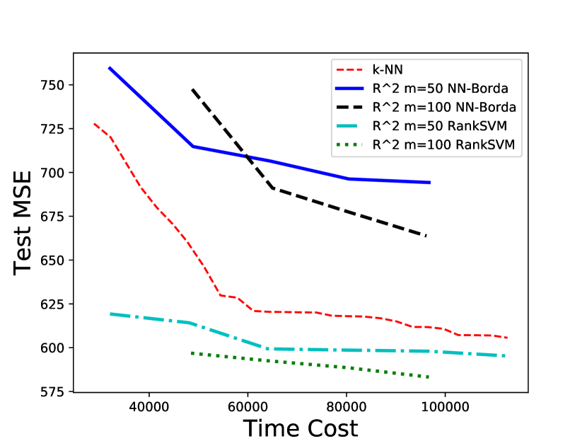
(b) Task 2

Figure 10: Experiments on AirBnB price estimation for nonparametric methods, using nearest neighbors of Borda count. Figure (a) uses 50-NN for averaging Borda counts, while Figure (b) uses 5-NN.

B Detailed Proofs

B.1 Proof of Theorem 1

Without loss of generality we assume throughout the proof that we re-arrange the samples so that the true ranking of the samples $\pi$ is the identity permutation, i.e. that $f(X_{1})\leq f(X_{2})\leq\ldots\leq f(X_{n})$. We let $C,c,C_{1},c_{1},\ldots$ denote universal positive constants. As is standard in nonparametric regression these constants may depend on the dimension $d$ but we suppress this dependence.

For a random point $X\in\mathcal{X}$, let $X_{\alpha}$ be the nearest neighbor of $X$ in the labeled set $\mathcal{L}$. We decompose the MSE as

$$\mathbb{E}\left[(\widehat{f}(X)-f(X))^{2}\right] \leq 2\mathbb{E}\left[(\widehat{f}(X)-f(X_{\alpha}))^{2}\right]+2\mathbb{E}\left[(f(X_{\alpha})-f(X))^{2}\right].$$

Under the assumptions of the theorem we have the following two results which provide bounds on the two terms in the above decomposition.

Lemma 12

For a constant $C>0$ we have that,

$$\mathbb{E}\left[(f(X_{\alpha})-f(X))^{2}\right]\leq Cn^{-2s/d}.$$

Lemma 13

For any $0<\delta\leq 1/2$ we have that there is a constant $C>0$ such that:

$$\mathbb{E}\left[(\widehat{f}(X)-f(X_{\alpha}))^{2}\right]\leq 4\delta M^{2}+$$

$$\frac{C\log(m/\delta)\log n\log(1/\delta)}{m}\left[\sum_{k=1}^{m}\left(\mathbb{E}\left[(\widehat{y}_{t_{k}}-f(X_{t_{k}}))^{2}\right]\right)+\sum_{k=0}^{m}\left(\mathbb{E}\left[(f(X_{t_{k+1}})-f(X_{t_{k}}))^{2}\right]\right)\right].$$

Taking these results as given we can now complete the proof of the theorem. We first note that the first term in the upper bound in Lemma 13 is simply the MSE in an isotonic regression problem, and using standard risk bounds for isotonic regression (see for instance, Theorem 2.2 in Zhang (2002)) we obtain that for a constant $C>0$:

$$\sum_{k=1}^{m}\mathbb{E}\left[(\widehat{y}_{t_{k}}-f(X_{t_{k}}))^{2}\right]\leq Cm^{2/3}.$$

Furthermore, since $f(X_{t_{m+1}})-f(X_{t_{0}})\leq 2M$, and the function values are increasing we obtain that:

$$\sum_{k=0}^{m}\left(\mathbb{E}\left[(f(X_{t_{k+1}})-f(X_{t_{k}}))^{2}\right]\right)\leq 4M^{2}.$$

Now, choosing $\delta=\max\{n^{-2s/d},1/m\}$ we obtain:

$$\mathbb{E}\left[(\widehat{f}(X)-f(X))^{2}\right] \leq C_{1}m^{-2/3}\log^{2}n\log m+C_{2}n^{-2s/d},$$

as desired. We now prove the two technical lemmas to complete the proof.

B.1.1 Proof of Lemma 12

The proof of this result is an almost immediate consequence of the following result from Györfi et al. (2006).

Lemma 14 (Györfi et al. (2006), Lemma 6.4 and Exercise 6.7)

Suppose that there exist positive constants $p_{\min}$ and $p_{max}$ such that $p_{\min}\leq p(x)\leq p_{\max}$. Then, there is a constant $c>0$, such that

$$\mathbb{E}[\|X_{\alpha}-X\|_{2}^{2}]\leq cn^{-2/d}.$$

Using this result and the Hölder condition we have

$$\mathbb{E}\left[(f(X_{\alpha})-f(X))^{2}\right] \leq L\mathbb{E}\left[\|X_{\alpha}-X\|_{2}^{2s}\right]$$

$$\stackrel{{\scriptstyle\text{(i)}}}{{\leq}}L\left(\mathbb{E}\left[\|X_{\alpha}-X\|_{2}^{2}\right]\right)^{s}$$

$$\leq cn^{-2s/d},$$

where (i) uses Jensen’s inequality. We now turn our attention to the remaining technical lemma.

B.1.2 Proof of Lemma 13

We condition on a certain favorable configuration of the samples that holds with high-probability. For a sample $\{X_{1},\ldots,X_{n}\}$ let us denote by

$$q_{i}:=\mathbb{P}(X_{\alpha}=X_{i}),$$

where $X_{\alpha}$ is the nearest neighbor of $X$. Furthermore, for each $k$ we recall that since we have re-arranged the samples so that $\pi$ is the identity permutation we can measure the distance between adjacent labeled samples in the ranking by $t_{k}-t_{k+1}.$ The following result shows that the labeled samples are roughly uniformly spaced (up to a logarithmic factor) in the ranked sequence, and that each point $X_{i}$ is roughly equally likely (up to a logarithmic factor) to be the nearest neighbor of a randomly chosen point.

Lemma 15

There is a constant $C>0$ such that with probability at least $1-\delta$ we have that the following two results hold:

1. We have that,

   $$\max_{1\leq j\leq n}q_{i}\leq\frac{Cd\log(1/\delta)\log n}{n}.$$ (9)

2. Let us take $t_{m+1}:=n+1$, then

   $$\max_{k\in[m+1]}t_{k}-t_{k-1}\leq\frac{Cn\log(m/\delta)}{m}.$$ (10)

Denote the event, which holds with probability at least $1-\delta$ in the above Lemma by $\mathcal{E}_{0}$. By conditioning on $\mathcal{E}_{0}$ we obtain the following decomposition:

$$\mathbb{E}\left[(\widehat{f}(X)-f(X_{\alpha}))^{2}\right] \leq~{}\mathbb{E}\left[(\widehat{f}(X)-f(X_{\alpha}))^{2}|\mathcal{E}_{0}\right]+\delta\cdot 4M^{2}$$

because both $f$ and $\widehat{f}$ are bounded in $[-M,M]$. We condition all calculations below on $\mathcal{E}_{0}$. Now we have

$$\mathbb{E}\left[(\widehat{f}(X)-f(X_{\alpha}))^{2}|\mathcal{E}_{0}\right] =\sum_{i=1}^{n}\mathbb{P}[X_{\alpha}=X_{i}|\mathcal{E}_{0}]\mathbb{E}\left[(\widehat{f}(X_{i})-f(X_{i}))^{2}|\mathcal{E}_{0}\right]$$

$$\leq\sum_{i=1}^{n}\max_{1\leq j\leq n}\mathbb{P}[X_{\alpha}=X_{j}|\mathcal{E}_{0}]\mathbb{E}\left[(\widehat{y}_{i}-f(X_{i}))^{2}|\mathcal{E}_{0}\right]$$

$$\leq\frac{Cd\log(1/\delta)\log n}{n}\sum_{i=1}^{n}\mathbb{E}\left[(\widehat{y}_{\widetilde{i}}-f(X_{i}))^{2}|\mathcal{E}_{0}\right],$$ (11)

where we recall that $\widehat{y}_{\widetilde{i}}$ (defined in Algorithm 1) denotes the de-noised (by isotonic regression) $y$ value at the nearest labeled left-neighbor of the point $X_{i}$.

For convenience we define $f(X_{t_{0}})=0$ (equivalently as in Algorithm 1 we are assigning a 0 value to any point with no labeled point with a smaller function value according to the permutation $\widehat{\pi}$). With this definition in place we have that,

$$\sum_{i=1}^{n}\mathbb{E}\left[(\widehat{y}_{\widetilde{i}}-f(X_{i}))^{2}|\mathcal{E}_{0}\right]$$

$$\leq \sum_{i=1}^{n}\left(2\mathbb{E}\left[(\widehat{y}_{\widetilde{i}}-f(X_{\widetilde{i}}))^{2}|\mathcal{E}_{0}\right]+2\mathbb{E}\left[(f(X_{i})-f(X_{\widetilde{i}}))^{2}|\mathcal{E}_{0}\right]\right)$$

$$= \sum_{i=1}^{n}\sum_{k=0}^{m}\mathbb{I}[\widetilde{i}=t_{k}]\left(2\mathbb{E}\left[(\widehat{y}_{t_{k}}-f(X_{t_{k}}))^{2}|\mathcal{E}_{0}\right]\mathbb{I}[k\neq 0]+2\mathbb{E}\left[(f(X_{i})-f(X_{t_{k}}))^{2}|\mathcal{E}_{0}\right]\right)$$

$$\stackrel{{\scriptstyle\text{(i)}}}{{\leq}} \sum_{i=1}^{n}\sum_{k=0}^{m}\mathbb{I}[\widetilde{i}=t_{k}]\left(2\mathbb{E}\left[(\widehat{y}_{t_{k}}-f(X_{t_{k}}))^{2}|\mathcal{E}_{0}\right]\mathbb{I}[k\neq 0]+2\mathbb{E}\left[(f(X_{t_{k+1}})-f(X_{t_{k}}))^{2}|\mathcal{E}_{0}\right]\right)$$

$$\stackrel{{\scriptstyle\text{(ii)}}}{{=}} \sum_{k=0}^{m}\left(2\mathbb{E}\left[(\widehat{y}_{t_{k}}-f(X_{t_{k}}))^{2}|\mathcal{E}_{0}\right]\mathbb{I}[k\neq 0]+2\mathbb{E}\left[(f(X_{t_{k+1}})-f(X_{t_{k}}))^{2}|\mathcal{E}_{0}\right]\right)\sum_{i=1}^{n}\mathbb{I}[\widetilde{i}=t_{k}]$$

$$\stackrel{{\scriptstyle\text{(iii)}}}{{\leq}} \frac{Cn\log(m/\delta)}{m}\sum_{k=1}^{m}\left(2\mathbb{E}\left[(\widehat{y}_{t_{k}}-f(X_{t_{k}}))^{2}|\mathcal{E}_{0}\right]\right)+\frac{Cn\log(m/\delta)}{m}\sum_{k=0}^{m}\left(2\mathbb{E}\left[(f(X_{t_{k+1}})-f(X_{t_{k}}))^{2}|\mathcal{E}_{0}\right]\right)$$

$$\leq \frac{2Cn\log(m/\delta)}{m}\left[\sum_{k=1}^{m}\left(\mathbb{E}\left[(\widehat{y}_{t_{k}}-f(X_{t_{k}}))^{2}|\mathcal{E}_{0}\right]\right)+\sum_{k=0}^{m}\left(\mathbb{E}\left[(f(X_{t_{k+1}})-f(X_{t_{k}}))^{2}|\mathcal{E}_{0}\right]\right)\right].$$

The inequality (i) follows by noticing that if $\widetilde{i}=t_{k}$, $f(X_{i})-f(X_{\widetilde{i}})$ is upper bounded by $f(X_{t_{k+1}})-f(X_{t_{k}})$. We interchange the order of summations to obtain the inequality (ii). The inequality in (iii) uses Lemma 15. We note that,

$$\mathbb{E}\left[(\widehat{y}_{t_{k}}-f(X_{t_{k}}))^{2}|\mathcal{E}_{0}\right]\leq\frac{\mathbb{E}\left[(\widehat{y}_{t_{k}}-f(X_{t_{k}}))^{2}\right]}{\mathbb{P}(\mathcal{E}_{0})}\leq 2\mathbb{E}\left[(\widehat{y}_{t_{k}}-f(X_{t_{k}}))^{2}\right],$$

since $\delta\leq 1/2$, and a similar manipulation for the second term yields that,

$$\sum_{i=1}^{n}\mathbb{E}\left[(\widehat{y}_{\widetilde{i}}-f(X_{i}))^{2}|\mathcal{E}_{0}\right]\leq \frac{4Cn\log(m/\delta)}{m}\left[\sum_{k=1}^{m}\mathbb{E}\left[(\widehat{y}_{t_{k}}-f(X_{t_{k}}))^{2}\right]+\sum_{k=0}^{m}\mathbb{E}\left[(f(X_{t_{k+1}})-f(X_{t_{k}}))^{2}\right]\right].$$

Plugging this expression back in to (11) we obtain the Lemma. Thus, to complete the proof it only remains to establish the result in Lemma 15.

B.1.3 Proof of Lemma 15

We prove each of the two results in turn.

Proof of Inequality (9): As a preliminary, we need the following Vapnik-Cervonenkis result from Chaudhuri and Dasgupta (2010):

Lemma 16

Suppose we draw a sample $\{X_{1},\ldots,X_{n}\}$, from a distribution $\mathbb{P}$, then there exists a universal constant $C^{\prime}$ such that with probability $1-\delta$, every ball $B$ with probability:

$$\mathbb{P}(B)\geq\frac{C^{\prime}\log(1/\delta)d\log n}{n},$$

contains at least one of the sample points.

We now show that under this event we have

$$\max_{i}q_{i}\leq\frac{C^{\prime}p_{\max}\log(1/\delta)d\log n}{p_{\min}n}.$$

Fix any point $X_{i}\in T$, and for a new point $X$, let $r=\|X_{i}-X\|_{2}$. If $X_{i}$ is $X$’s nearest neighbor in $T$, there is no point in the ball $B(X,r)$. Comparing this with the event in Lemma 16 we have

$$p_{\min}v_{d}r^{d}\leq\frac{C^{\prime}\log(1/\delta)d\log n}{n},$$

where $v_{d}$ is the volume of the unit ball in $d$ dimension.

Hence we obtain an upper bound on $r$. Now since $p(x)$ is upper and lower bounded we can bound the largest $q_{i}$ as

$$\max_{i}q_{i}\leq p_{\max}v_{d}r^{d}\leq\frac{C^{\prime}p_{\max}\log(1/\delta)d\log n}{p_{\min}n}.$$

Thus we obtain the inequality (9).

Proof of Inequality (10): Recall that we define $t_{m+1}:=n+1.$ Notice that $t_{1},\ldots,t_{m}$ are randomly chosen from $[n]$. So for each $k\in[m]$ we have

$$\mathbb{P}[t_{k}-t_{k-1}\geq t]\leq\frac{n-t+1}{n}\left(\frac{n-t}{n}\right)^{m-1}\leq\left(\frac{n-t}{n}\right)^{m-1},$$

since we must randomly choose $t_{k}$ in $X_{t},X_{t+1},\ldots,X_{n}$, and choose the other $m-1$ samples in $X_{1},\ldots,X_{t_{k}-t},X_{t_{k}+1},\ldots,X_{n}$. Similarly we also have

$$\mathbb{P}[t_{m+1}-t_{m}\geq t]\leq\left(\frac{n-t}{n}\right)^{m-1}.$$

So

$$\mathbb{P}[\max_{k\in[m+1]}t_{k}-t_{k-1}\geq t] \leq\sum_{k=1}^{m+1}\mathbb{P}[\max_{k\in[m+1]}t_{k}-t_{k-1}\geq t]$$

$$\leq(m+1)\left(\frac{n-t}{n}\right)^{m-1}.$$

Setting this to be less than or equal to $\delta$, we have

$$\frac{t}{n}\geq{1-\left(\frac{\delta}{m+1}\right)^{\frac{1}{m-1}}}.$$

Let $u=\log\left(1-\left(\frac{\delta}{m+1}\right)^{\frac{1}{m-1}}\right)=-C\frac{\log(m/\delta)}{m}$, we have $1-e^{u}=O(-u)$ since $u$ is small and bounded. So it suffices for $t\geq C\frac{n\log(m/\delta)}{m}$ such that

$$\mathbb{P}[\max_{k\in[m+1]}t_{k}-t_{k-1}\geq t]\leq\delta.$$

B.2 Proof of Theorem 2

To prove the result we separately establish lower bounds on the size of the labeled set of samples $m$ and the size of the ordered set of samples $n$. Concretely, we show the following pair of claims, for a positive constant $C>0$,

$$\inf_{\widehat{f}}\sup_{f\in\mathcal{F}_{s,L}}\mathbb{E}\left[(f(X)-\widehat{f}(X))^{2}\right]\geq Cm^{-2/3}$$ (12)

$$\inf_{\widehat{f}}\sup_{f\in\mathcal{F}_{s,L}}\mathbb{E}\left[(f(X)-\widehat{f}(X))^{2}\right]\geq Cn^{-2s/d}.$$ (13)

We prove each of these claims in turn and note that together they establish Theorem 2.

Proof of Claim (12): We establish the lower bound in this case by constructing a suitable packing set of functions, and using Fano’s inequality. The main technical novelty, that allows us to deal with the setting where both direct and ordinal information is available, is that we construct functions that are all increasing functions of the first covariate $x_{1}$, and for these functions the ordinal measurements provide no additional information.

Without loss of generality we consider the case when $d=1$, and note that the claim follows in general by simply extending our construction using functions for which $f(x)=f(x_{1})$. We take the covariate distribution $\mathbb{P}_{\mathcal{X}}$ to be uniform on $[0,1]$. For a kernel function $K$ that is $1$-Lipschitz on $\mathbb{R}$, bounded and supported on $[-1/2,1/2]$, with

$$\int_{-1/2}^{1/2}K^{2}(x)dx>0$$

we define:

$$u =\lceil m^{\frac{1}{3}}\rceil,~{}~{}~{}h=1/u,$$

$$x_{k} =\frac{k-1/2}{u},~{}~{}~{}\phi_{k}(x)=\frac{Lh}{2}K\left(\frac{x-x_{k}}{h}\right),~{}~{}~{}\text{for}~{}~{}~{}k=\{1,2,\ldots,u\},$$

$$\Omega =\{\omega:\omega\in\{0,1\}^{u}\}.$$

With these definitions in place we consider the following class of functions:

$$\mathcal{G}=\left\{f_{\omega}:[0,1]\mapsto\mathbb{R}:f_{\omega}(x)=\frac{Lx}{2}+\sum_{i=1}^{k}\omega_{i}\phi_{i}(x),~{}\text{for}~{}x\in[0,1]\right\}.$$

We note that the functions in $\mathcal{G}$ are $L$-Lipschitz, and thus satisfy the Hölder constraint (for any $0<s\leq 1$).

We note that these functions are all increasing so the permutation $\pi$ contains no additional information and can be obtained simply by sorting the samples (according to their first coordinate). Furthermore, in this case the unlabeled samples contribute no additional information as their distribution $\mathbb{P}_{\mathcal{X}}$ is known (since we take it to be uniform). Concretely, for any estimator in our setup which uses $\{(X_{1},y_{1}),\ldots,(X_{m},y_{m}),X_{m+1},\ldots,X_{n},\pi\}$ with

$$\sup_{f\in\mathcal{G}}\mathbb{E}\left[(f(X)-\widehat{f}(X))^{2}\right]<Cm^{-2/3},$$

we can construct an equivalent estimator that uses only $\{(X_{1},y_{1}),\ldots,(X_{m},y_{m})\}$. In particular, we can simply augment the sample by sampling $X_{m+1},\ldots,X_{n}$ uniformly on $[0,1]$ and generating $\pi$ by ranking $X$ in increasing order.

In light of this observation, in order to complete the proof of Claim (12) it sufficies to show that $Cm^{-2/3}$ is a lower bound for estimating functions in $\mathcal{G}$ with access to only noisy labels. For any pair $\omega,\omega^{\prime}\in\Omega$ we have that,

$$\mathbb{E}[(f_{\omega}(X)-f_{\omega^{\prime}}(X))^{2}] =\sum_{k=1}^{u}(\omega_{k}-\omega_{k}^{\prime})^{2}\int\phi^{2}_{k}(x)dx$$

$$=L^{2}h^{3}\|K\|^{2}_{2}\rho(\omega,\omega^{\prime}),$$

where $\rho(\omega,\omega^{\prime})$ denotes the hamming distance between $x$ and $x^{\prime}$.

Denote by $P_{0}$ the distribution induced by the function $f_{0}$ with $\omega=(0,\ldots,0)$, with the covariate distribution being uniform on $[0,1].$ We can upper bound the KL divergence between the distribution induced by any function in $\mathcal{G}$ and $P_{0}$ as:

$$\text{KL}(P_{j}^{m},P_{0}^{m}) =m\int_{\mathcal{X}}p(x)\int_{\mathbb{R}}p_{j}(y|x)\log\frac{p_{0}(y|x)}{p_{j}(y|x)}dydx$$

$$=m\int_{\mathcal{X}}p(x)\sum_{i=1}^{u}\omega^{j}_{i}\phi^{2}_{i}(x)dx$$

$$\leq mL^{2}h^{3}\|K\|^{2}_{2}u.$$

Now, the Gilbert-Varshamov bound (Varshamov, 1957; Gilbert, 1952), ensures that if $u>8$, then there is a subset $\Omega^{\prime}\subseteq\Omega$ of cardinality $2^{u/8}$, such that the Hamming distance between each pair of elements $\omega,\omega^{\prime}\in\Omega^{\prime}$ is at least $u/8$. A straightforward application of Fano’s inequality (see for instance Theorem 2.5 in Tsybakov (2009)) shows that for small constants $c,c^{\prime}>0$, if:

$$mL^{2}h^{3}\|K\|^{2}_{2}u\leq cu,$$

then the error of any estimator is lower bounded as:

$$\sup_{f\in\mathcal{G}}\mathbb{E}[(\widehat{f}(X)-f(X))^{2}] \geq c^{\prime}L^{2}h^{3}\|K\|^{2}_{2}u\geq c^{\prime}m^{-2/3},$$

establishing the desired claim.

Proof of Claim (13): We show this claim by reducing to the case where we have $n$ points with noiseless evaluations, i.e., we observe $\{(X_{1},f(X_{1})),(X_{2},f(X_{2})),\ldots,(X_{n},f(X_{n}))\}$. We notice that the ranking $\pi$ provides no additional information when all the points are labeled without noise. Formally, if we have an estimator $\widehat{f}$ which when provided $\{(X_{1},y_{1}),\ldots,(X_{m},y_{m}),X_{m+1},\ldots,X_{n},\pi\}$ obtains an error less than $cn^{-2s/d}$ (for some sufficiently small constant $c>0$) then we can also use this estimator in setting where all $n$ samples are labeled without noise, by generating $\pi$ according to the noiseless labels, adding Gaussian noise to the labels of $m$ points, and eliminating the remaining labels before using the estimator $\widehat{f}$ on this modified sample.

It remains to show that, $cn^{-2s/d}$ is a lower bound on the MSE of any estimator that receives $n$ noiseless labels. To simplify our notation we will assume that $(2n)^{1/d}$ is an integer (if not we can establish the lower bound for a larger sample-size for which this condition is true, and conclude the desired lower bound with an adjustment of various constants). For a given sample size $n$, we choose

$$h =(2n)^{-1/d},$$

and consider the grid with $2n$ cubes with side-length $h$. Denote the centers of the cubes as $\{x_{1},\ldots,x_{2n}\}$. For a kernel function $K$ supported on $[-1/2,1/2]^{d}$, which is 1-Lipschitz on $\mathbb{R}^{d}$, bounded and satisfies:

$$\int_{[-1/2,1/2]^{d}}K^{2}(x)dx>0$$

we consider a class of functions:

$$\mathcal{G}=\left\{f_{\omega}:f_{\omega}(x)=Lh^{s}\sum_{i=1}^{2n}\omega_{i}K\left(\frac{x-x_{i}}{h}\right),\text{for}~{}\omega\in\{0,1\}^{2n}\right\}.$$

We note that these functions are all in the desired Hölder class with exponent $s$. Given $n$ samples (these may be arbitrarily distributed) $\{(X_{1},f(X_{1})),\ldots,(X_{n},f(X_{n}))\}$, we notice that we are only able to identify at most $n$ of the $\omega_{i}$ (while leaving at least $n$ of the $\omega_{i}$ completely unconstrained) and thus any estimator $\widehat{f}$ must incur a large error on at least one of the functions $f_{\omega}$ consistent with the obtained samples. Formally, we have that

$$\sup_{f\in\mathcal{G}}\mathbb{E}(\widehat{f}(X)-f(X))^{2}\geq\frac{nL^{2}h^{2s+d}\|K\|_{2}^{2}}{4}\geq cn^{-2s/d},$$

as desired. This completes the proof of Claim (13).

B.3 Proof of Theorem 3

Throughout this proof without loss of generality we re-arrange the samples so that the estimated permutation $\widehat{\pi}$ is the identity permutation. To simplify the notation further, we let $X_{(i)}=X_{\pi^{-1}(i)}$ be the $i$-th element according to true permutation $\pi$. This leads to $f(X_{(1)})\leq f(X_{(2)})\leq\cdots\leq f(X_{(n)})$.

We begin with a technical result that bounds the error of using $\widehat{\pi}$ instead of the true permutation $\pi$ in the R² algorithm.

The first part of the proof is the same as that of Theorem 1. We have

$$\mathbb{E}\left[(\widehat{f}(X)-f(X))^{2}\right] \leq 2\mathbb{E}\left[(\widehat{f}(X)-f(X_{\alpha}))^{2}\right]+2\mathbb{E}\left[(f(X_{\alpha})-f(X))^{2}\right]$$

$$\leq 2\mathbb{E}\left[(\widehat{f}(X)-f(X_{\alpha}))^{2}\right]+Cn^{-2s/d}.$$

And for event $\mathcal{E}_{0}$ we have (note that $\widetilde{i}$ is the nearest neighbor index defined in Algorithm 1)

$$\mathbb{E}\left[(\widehat{f}(X)-f(X_{\alpha}))^{2}\right] \leq C\frac{d\log(1/\delta)\log n}{n}\sum_{i=1}^{n}\mathbb{E}\left[(\widehat{y}_{\widetilde{i}}-f(X_{i}))^{2}|\mathcal{E}_{0}\right]+\delta$$

$$\leq C\left(\frac{\log^{2}n}{n}\sum_{i=1}^{n}\mathbb{E}\left[(\widehat{y}_{\widetilde{i}}-f(X_{i}))^{2}|\mathcal{E}_{0}\right]+n^{-2s/d}\right).$$ (14)

The second inequality is obtained by letting $\delta=n^{-2s/d}$. To bound the sum of expectations above, we first prove a lemma bounding the difference between $X_{1},\ldots,X_{n}$ and $X_{(1)},\ldots,X_{(n)}$:

Lemma 4(Restated). Suppose the ranking $(X_{1},\ldots,X_{n})$ is of at most $\nu$ error with respect to the true permutation. Then

$$\sum_{i=1}^{n}(f(X_{i})-f(X_{(i)})^{2}\leq 8M^{2}\sqrt{2\nu}n.$$

Proof  Let $\theta_{i}=f(X_{i})$ and $\theta_{(i)}=f(X_{(i)})$, and let $g(\theta_{1},\ldots,\theta_{n})=\sum_{i=1}^{n}(\theta_{i}-\theta_{(i)})^{2}$. Consider $g$ as a function of $\theta_{i}$; $\theta_{i}$ appears twice in $g$, one as $(\theta_{i}-\theta_{(i)})^{2}$, and the other as $(\theta_{\pi(i)}-\theta_{(\pi(i))})^{2}=(\theta_{\pi(i)}-\theta_{i})^{2}$. If $\pi(i)=i$, then $\theta_{i}$ does not influence value of $g$; otherwise, $g$ is a quadratic function of $\theta_{i}$, and it achieves maximum either when $\theta_{i}=M$ or $\theta_{i}=-M$. So when $g$ achieves maximum it must be $\theta_{i}\in\{-M,M\}$. Now notice that $\theta_{(1)}\leq\cdots\leq\theta_{(n)}$, so the maximum is achieved when for some $0\leq k\leq n$ that $\theta_{(i)}=-M$ for $i\leq k$, and $\theta_{(i)}=M$ for $i>k$.

Note that $\sum_{i=1}^{n}(\theta_{i}-\theta_{(i)})^{2}=\sum_{i=1}^{n}(\theta_{\pi^{-1}(i)}-\theta_{(\pi^{-1}(i))})^{2}=\sum_{i=1}^{n}(\theta_{(i)}-\theta_{(\pi^{-1}(i))})^{2}$. From the discussion above, in the maximum case $(\theta_{(i)}-\theta_{(\pi^{-1}(i))})^{2}=4M^{2}$ iff $i$ and $\pi^{-1}(i)$ lies on different sides of $k$, and otherwise it is 0. To further bound the sum, we use the Spearman Footrule distance between $\pi$ and $(1,2,\ldots,n)$, which Diaconis and Graham (1977) shows that it can be bounded as

$$\sum_{i=1}|\pi(i)-i|\leq 2\sum_{1\leq i,j\leq n}I\left[(\pi(i)-\pi(j))(i-j)<0\right].$$

And the RHS can be bounded by $2\nu n^{2}$ since the agnostic error of ranking is at most $\nu$. We also have that

$$\sum_{i=1}|\pi(i)-i|=\sum_{i=1}|\pi(\pi^{-1}(i))-\pi^{-1}(i)|=\sum_{i=1}|i-\pi^{-1}(i)|.$$

Let $U_{1}=\{i:\pi^{-1}(i)\leq k,i>k\}$ and $U_{2}=\{\pi^{-1}(i)>k,i\leq k\}$. So in the maximum case we have

$$\sum_{i=1}^{n}(\theta_{\pi(i)}-\theta_{i})^{2}=4M^{2}(|U_{1}|+|U_{2}|).$$

Now notice that for $i\in U_{1}$, we have $|\pi^{-1}(i)-i|\geq i-k$; and for $i\in U_{2}$ we have$|\pi^{-1}(i)-i|\geq k-i+1$. Considering the range of $i$ we have

$$\sum_{j=1}^{|U_{1}|}j+\sum_{j=1}^{|U_{2}|}j\leq\sum_{i=1}^{n}|\pi^{-1}(i)-i|\leq 2\nu n^{2}.$$

So $|U_{1}|+|U_{2}|\leq 2\sqrt{2\nu}n$. And

$$\sum_{i=1}^{n}(f(X_{i})-f(X_{(i)})^{2}=\sum_{i=1}^{n}(\theta_{\pi(i)}-\theta_{i})^{2}\leq 4M^{2}(|U_{1}|+|U_{2}|)\leq 8M^{2}\sqrt{2\nu}n.$$

Thus we prove the lemma.  

Now back to the original proof. Under event $\mathcal{E}_{0}$ we have

$$\sum_{i=1}^{n}E[(\widehat{y}_{i}-f(X_{i}))^{2}|\mathcal{E}_{0}]$$

$$= \sum_{i=1}^{n}E[(\widehat{y}_{\widetilde{i}}-f(X_{i}))^{2}|\mathcal{E}_{0}]$$

$$\leq \sum_{i=1}^{n}\mathbb{E}\left[2(\widehat{y}_{\widetilde{i}}-f(X_{\widetilde{i}}))^{2}+2(f(X_{\widetilde{i}})-f(X_{i}))^{2}|\mathcal{E}_{0}\right]$$

$$\leq \frac{Cn\log(m/\delta)}{m}\sum_{k=1}^{m}\mathbb{E}\left[(\widehat{y}_{t_{k}}-f(X_{t_{k}}))^{2}|\mathcal{E}_{0}\right]+2\sum_{i=1}^{n}\mathbb{E}\left[(f(X_{\widetilde{i}})-f(X_{i}))^{2}|\mathcal{E}_{0}\right].$$ (15)

We omit the condition $\mathcal{E}_{0}$ in discussion below. We bound the two terms separately. For the first term, we use the following theorem adapted from Zhang (2002):

Theorem 17 (Zhang (2002), adapted from Theorem 2.3 and Remark 4.2)

Suppose $X_{t_{k}},y_{t_{k}}$ are fixed for $k\in[m]$, and $f(X_{t_{k}})$ is arbitrary in order. Let

$$S=\min_{u}\sum_{k=1}^{m}(u_{k}-f(X_{t_{k}}))^{2},$$

where the minimum is taken over all sequence of $u\in\mathbb{R}^{m}$ that is non-decreasing. The risk of isotonic regression satisfies

$$\frac{1}{m^{2/3}M^{1/3}}\left(\mathbb{E}\left[\sum_{k=1}^{m}(\widehat{y}_{t_{k}}-f(X_{t_{k}}))^{2}\right]-S\right)\leq C$$

for some universal constant $C$.

So from Theorem 17 we know that

$$\mathbb{E}\left[(\widehat{y}_{t_{k}}-f(X_{t_{k}}))^{2}\right]\leq\mathbb{E}[S]+Cm^{1/3},$$

where the expectation in $E[S]$ is taken w.r.t. the randomness in $t_{k}$. From Lemma 4 we know that

$$\sum_{i=1}^{n}(f(X_{i})-f(X_{(i)}))^{2}\leq C\sqrt{\nu}n.$$

Note that since $t_{k}$ is taken at random, each element $X_{i}$ has equal probability $\frac{m}{n}$ to be picked; so

$$\mathbb{E}[S]\leq\mathbb{E}\left[\sum_{i=1}^{m}(f(X_{(t_{k})})-f(X_{t_{k}}))^{2}\right]\leq C\sqrt{\nu}m.$$

Now we bound the second term in (15). We have

$$\sum_{i=1}^{n}\mathbb{E}\left[(f(X_{\widetilde{i}})-f(X_{i}))^{2}\right]$$

$$\leq \;3\sum_{i=1}^{n}\mathbb{E}\left[(f(X_{\widetilde{i}})-f(X_{(\widetilde{i})}))^{2}\right]+3\sum_{i=1}^{n}\mathbb{E}\left[(f(X_{(\widetilde{i})})-f(X_{(i)}))^{2}\right]+3\sum_{i=1}^{n}\mathbb{E}\left[(f(X_{(i)})-f(X_{i}))^{2}\right]$$

$$\leq \;\frac{Cn\log m}{m}\sum_{k=1}^{m}\mathbb{E}\left[(f(X_{t_{k}})-f(X_{(t_{k})}))^{2}\right]+\frac{Cn\log m}{m}\sum_{k=1}^{m}\mathbb{E}\left[(f(X_{(t_{k+1})})-f(X_{(t_{k})}))^{2}\right]$$

$$\;~{}~{}~{}~{}~{}~{}~{}~{}~{}~{}~{}~{}~{}~{}+3\sum_{i=1}^{n}\mathbb{E}\left[(f(X_{(i)})-f(X_{i}))^{2}\right]$$

$$\leq ~{}\frac{Cn\log m}{m}\sqrt{\nu}m+\frac{Cn\log m}{m}\cdot 1+C\sqrt{\nu}n$$

$$= ~{}C\sqrt{\nu}n\log m.$$

The first inequality is by noticing $(x+y+z)^{2}\leq 3x^{2}+3y^{2}+3z^{2}$ for any number $x,y,z\in\mathbb{R}$; the second inequality is by grouping values of $\widetilde{i}$, and the choice of $t_{k}$; the third inequality comes from analysis of the first term on $\sum_{k=1}^{m}\mathbb{E}\left[(f(X_{t_{k}})-f(X_{(t_{k})}))^{2}\right]$, the fact that $f(X_{(t_{m})})-f(X_{(t_{1})})\leq 1$, and Lemma 4.

Summarizing the two terms we have

$$\mathbb{E}\left[(\widehat{y}_{\widetilde{i}}-f(X_{i}))^{2}|\mathcal{E}_{0}\right]\leq C(\sqrt{\nu}n+m^{-2/3}n)\log m.$$

Take this back to (14) we prove the theorem.

B.4 Proof of Theorem 5

To simplify notation, we suppose that we have $m$ labeled samples $T=\{(X_{i},y_{i})\}_{i=1}^{m}$ for training and another $m$ labeled samples $V=\{(X_{i},y_{i})\}_{i=m+1}^{2m}$ for validation. We consider the following models:

1. R² using both the ordinal data and the labeled samples in $T$, and we denote by $\widehat{f}_{0}$,

2. $k$-NN regression using only the labeled samples in $T$ for $k\in[m]$ which we denote by $\{\widehat{f}_{1},\ldots,\widehat{f}_{m}\}$.

We select the best model according to performance on validation set. We further restrict all estimators to be bounded in $[-M,M]$; i.e., when $\widehat{f}_{j}(x)<-M$ for some $x$ and $j$, we clip its value by setting $\widehat{f}_{j}(x)=-M$ and we analogously clip the function when it exceeds $M$. We note in passing that this only reduces the MSE since the true function $f$ is bounded between $[-M,M]$. Throughout the remainder of the proof we condition on the training set $T$ but suppress this in our notation. We define the empirical validation risk of a function $\widehat{f}$ to be:

$$\widehat{R}^{V}\big{(}\widehat{f}\big{)}=\frac{1}{m}\sum_{i=m+1}^{2m}\big{(}y_{i}-\widehat{f}(X_{i})\big{)}^{2},$$

and the population MSE of a function $\widehat{f}$ to be

$$\text{err}(\widehat{f})=\mathbb{E}\big{[}\big{(}\widehat{f}(X)-f(X)\big{)}^{2}\big{]},$$

where $\epsilon\sim N(0,1)$ denotes the noise in the direct measurements. Now let

$$\widehat{f}^{*}=\operatorname*{arg\,min}_{j=0,\ldots,m}\widehat{R}^{V}(\widehat{f}_{j}),$$

be the best model selected using cross validation and

$$f^{*}=\operatorname*{arg\,min}_{j=0,\ldots,m}\text{err}(\widehat{f}_{j}),$$

be the estimate with lowest MSE in $\widehat{f}_{0},\ldots,\widehat{f}_{m}$. Let us denote:

$$\mathcal{G}=\{\widehat{f}_{0},\ldots,\widehat{f}_{m}\}.$$

Recall that $f$ denotes the true unknown regression function. Then in the sequel we show the following result:

Lemma 18

With probability at least $1-\delta$, for any $\widehat{f}\in\mathcal{G}$ we have that the following hold for some constant $C>0$,

$$\text{err}(\widehat{f})\leq 2\left[\widehat{R}^{V}(\widehat{f})-\widehat{R}^{V}(f)\right]+\frac{C\log(m/\delta)}{m},$$ (16)

$$\left[\widehat{R}^{V}(\widehat{f})-\widehat{R}^{V}(f)\right]\leq 2\text{err}(\widehat{f})+\frac{C\log(m/\delta)}{m}.$$ (17)

Since $\widehat{R}^{V}(\widehat{f}^{*})\leq\widehat{R}^{V}(f^{*})$ we obtain using (16) that with probability at least $1-\delta$,

$$\text{err}(\widehat{f}^{*})\leq 2\left[\widehat{R}^{V}(f^{*})-\widehat{R}^{V}(f)\right]+\frac{C\log(m/\delta)}{m}.$$

Since $f^{*}\in\mathcal{G}$, we can use (17) to obtain that with probability $1-\delta$,

$$\text{err}(\widehat{f}^{*})\leq 4\text{err}(f^{*})+\frac{2C\log(m/\delta)}{m}.$$

Since $\text{err}(\widehat{f}^{*})$ is a positive random variable, integrating this bound we obtain that,

$$\mathbb{E}[\text{err}(\widehat{f}^{*})] =\int_{0}^{\infty}\mathbb{P}(\text{err}(\widehat{f}^{*})\geq t)dt,$$

$$\leq 4\text{err}(f^{*})+\frac{6C\log(m)}{m}.$$

So far we have implicitly conditioned throughout on the training set $T$. Taking an expectation over the training set yields:

$$\mathbb{E}[\text{err}(\widehat{f}^{*})]\leq 4\mathbb{E}[\text{err}(f^{*})]+\frac{6C\log(m)}{m}.$$

We now note that,

$$\mathbb{E}[\text{err}(f^{*})]]\leq\min_{j\in\{0,\ldots,m\}}\mathbb{E}[\text{err}(\widehat{f}_{j})].$$

Standard results on $k$-NN regression (for instance, a straightforward modification of Theorem 6.2 in Györfi et al. (2006) to deal with $0<s\leq 1$ in the Hölder class) yield that for a constant $C>0$,

$$\min_{j\in\{1,\ldots,m\}}\mathbb{E}[\text{err}(\widehat{f}_{j})]\leq Cm^{-2s/(2s+d)}.$$

Theorem 3 yields that,

$$\mathbb{E}[\text{err}(\widehat{f}_{0})]\leq C_{1}\left(\log^{2}n\log m\left(m^{-2/3}+\sqrt{\nu}\right)\right)+C_{2}n^{-2s/d},$$

and putting these together we obtain that,

$$\mathbb{E}[\text{err}(f^{*})]\leq\widetilde{O}\left(m^{-2/3}+\min\{\sqrt{\nu},m^{-\frac{2s}{2s+d}}\}+n^{-2s/d}\right),$$

and thus it only remains to prove Lemma 18 to complete the proof of the theorem.

B.4.1 Proof of Lemma 18

For a fixed classifier $\widehat{f}$ and for samples in the validation set $i\in\{m+1,\ldots,2m\}$ we define the random variables:

$$Z_{i}=(y_{i}-\widehat{f}(X_{i}))^{2}-(y_{i}-f(X_{i}))^{2}=(\widehat{f}(X_{i})-f(X_{i}))^{2}+2\epsilon_{i}(f(X_{i})-\widehat{f}(X_{i})),$$

and note that $\mathbb{E}[Z_{i}]=\text{err}(\widehat{f}).$ In order to obtain tail bounds on the average of the $Z_{i}$ let us bound the absolute central moments of $Z_{i}$. Using the inequality that $(x+y)^{k}\leq 2^{k-1}(x^{k}+y^{k})$, for $k>2$ we obtain that,

$$\mathbb{E}|Z_{i}-\mathbb{E}[Z_{i}]|^{k} =\mathbb{E}|(\widehat{f}(X_{i})-f(X_{i}))^{2}+2\epsilon_{i}(f(X_{i})-\widehat{f}(X_{i}))-\text{err}(\widehat{f})|^{k}$$

$$\leq 2^{k-1}\mathbb{E}|(\widehat{f}(X_{i})-f(X_{i}))^{2}-\text{err}(\widehat{f})|^{k}+2^{k-1}\mathbb{E}|\epsilon_{i}(f(X_{i})-\widehat{f}(X_{i}))|^{k}.$$ (18)

We bound each of these terms in turn. Since $(\widehat{f}(X_{i})-f(X_{i}))^{2}\in[0,4M^{2}]$, we obtain that,

$$\mathbb{E}|(\widehat{f}(X_{i})-f(X_{i}))^{2}-\text{err}(\widehat{f})|^{k}\leq\text{var}((\widehat{f}(X_{i})-f(X_{i}))^{2})(4M^{2})^{k-2},$$

and using the fact that $\epsilon_{i}$ are Gaussian we obtain that,

$$\mathbb{E}|\epsilon_{i}(f(X_{i})-\widehat{f}(X_{i}))|^{k} \leq\mathbb{E}|\epsilon_{i}|^{k-2}\mathbb{E}(f(X_{i})-\widehat{f}(X_{i}))^{2}(2M)^{k-2}$$

$$\leq\text{var}(\epsilon_{i}(f(X_{i})-\widehat{f}(X_{i})))k!\times(2M)^{k-2}.$$

Since $\epsilon_{i}$ is independent of the other terms in $Z_{i}$ we have that,

$$\text{var}(Z_{i})=\text{var}(\epsilon_{i}(f(X_{i})-\widehat{f}(X_{i})))+\text{var}((\widehat{f}(X_{i})-f(X_{i}))^{2}).$$

Putting these pieces together with (18) we obtain,

$$\mathbb{E}|Z_{i}-\mathbb{E}[Z_{i}]|^{k} \leq 2^{k-1}\text{var}(Z_{i})\left[k!\times(2M)^{k-2}+(4M^{2})^{k-2}\right]$$

$$\leq\frac{\text{var}(Z_{i})}{2}k!(16M+32M^{2})^{k-2}.$$

Let us denote $r:=16M+32M^{2}$. It remains to bound the variance. We have that,

$$\text{var}(Z_{i})\leq\mathbb{E}[Z_{i}^{2}]\leq 2\mathbb{E}((\widehat{f}(X_{i})-f(X_{i}))^{4})+8\mathbb{E}(f(X_{i})-\widehat{f}(X_{i}))^{2},$$

and using the fact that the functions are bounded in $[-M,M]$ we obtain that,

$$\text{var}(Z_{i})\leq(8M^{2}+8)\text{err}(\widehat{f}).$$ (19)

Now, applying the inequality in Lemma 23, we obtain that for any $c<1$ and for any $t\leq c/r$ that,

$$\text{err}(\widehat{f})\leq\frac{1}{m}\sum_{i=m+1}^{2m}Z_{i}+\frac{\log(1/\delta)}{mt}+\frac{8t(M^{2}+1)\text{err}(\widehat{f})}{2(1-c)},$$

we choose $c=1/2$ and $t=\min\{1/(2r),1/(16(M^{2}+1))\}$, and rearrange to obtain that,

$$\text{err}(\widehat{f})\leq\frac{2}{m}\sum_{i=m+1}^{2m}Z_{i}+\frac{2\log(1/\delta)}{m}\max\{2r,16(M^{2}+1)\}, \leq\frac{2}{m}\sum_{i=m+1}^{2m}Z_{i}+\frac{C\log(1/\delta)}{m},$$

and using a union bound over the $m+1$ functions $\widehat{f}\in\mathcal{G}$ we obtain (16). Repeating this argument with the random variables $-Z_{i}$ we obtain (17) completing the proof of the Lemma.

B.5 Proof of Theorem 6

We prove a slightly stronger result, and show Theorem 6 as a corollary.

Theorem 19

Assume the same modeling assumptions for $X_{1},\ldots,X_{n},y_{1},\ldots,y_{m}$ as in Theorem 2. Also permutation $\widehat{\pi}$ satisfies $\mathbb{P}[(f(X_{i})-f(X_{j}))(\pi(i)-\pi(j))<0]\leq\nu$. Then for any estimator $\widehat{f}$ taking input $X_{1},\ldots,X_{n},y_{1},\ldots,y_{m}$ and $\widehat{\pi}$, we have

$$\inf_{\widehat{f}}\sup_{f\in\mathcal{F}_{s,L}}\mathbb{E}\big{(}f(X)-\widehat{f}(X)\big{)}^{2}\geq C(m^{-\frac{2}{3}}+\min\{\nu^{\frac{d+2}{2d}}m^{\frac{1}{2d}},1\}m^{-\frac{2}{d+2}}+n^{-2s/d}).$$

Proof of Theorem 19  In this proof, we use $x_{i}$ to represent $i$-th dimension of $x$, and upper script for different vectors $x^{(1)},x^{(2)},\ldots$. Let $u=\lceil m^{\frac{1}{2+d}}\rceil,h=1/u$, and $t=\min\left\{\left(\nu m^{\frac{1}{2+d}}\right)^{\frac{1}{2d}},1\right\}$. Let $\Gamma=\{(\gamma_{1},\ldots,\gamma_{d}),\gamma_{i}\in\{1,2,\ldots,u\}\}$. Choose an arbitrary order on $\Gamma$ to be $\Gamma=\{\gamma^{(1)},\ldots,\gamma^{(u^{d})}\}$. Let $x^{(k)}=\frac{\gamma^{(k)}-1/2}{u}$, and $\phi_{k}(x)=\frac{L}{2}thK(\frac{x-tx^{(k)}}{th}),k=1,2,\ldots,u^{d}$, where $K$ is a kernel function in $d$ dimension supported on $[-1/2,1/2]^{d}$, i.e., $\int K(x)dx$ and $\max_{x}K(x)$ are both bounded, $K$ is 1-Lipschitz. So $\phi_{k}(x)$ is supported on $[thx^{(k)}-1/2th,thx^{(k)}+1/2th]$. Let $\Omega=\{\omega=(\omega_{1},\ldots,\omega_{u^{d}}),\omega_{i}\in\{0,1\}\}$, and

$$\mathcal{E}=\left\{f_{\omega}(x)=\frac{L}{2}x_{1}+\sum_{i=1}^{k}\omega_{i}\phi_{k}(x),x\in[0,1]^{d}\right\}.$$

Functions in $\mathcal{E}$ are $L$-Lipschitz. The function value is linear in $x_{1}$ for $x\not\in[0,t]^{d}$ in all functions in $\mathcal{E}$. Consider the comparison function $Z(x,x^{\prime})=I(x_{1}<x_{1}^{\prime})$ that ranks $x$ according to the first dimension. Since $K$ is 1-Lipschitz, it only makes an error when both $x,x^{\prime}$ lies in $[0,t]^{d}$, and both $x_{1},x_{1}^{\prime}$ lie in the same grid segment $[tk/u,t(k+1)/u]$ for some $k\in[u]$. So the error is at most $t^{2d}(1/u)^{2}\cdot u\leq\nu$ for any function $f\in\mathcal{E}$. Thus, if there exists one estimator with $\sup_{f}\mathbb{E}[(f-\widehat{f})^{2}]<C\min\{\nu^{\frac{d+2}{2d}}m^{\frac{1}{2d}},1\}m^{-\frac{2}{d+2}}$, then we can obtain one estimator for functions in $\mathcal{E}$ by using $\widehat{f}$ on $\mathcal{E}$, and responding to all comparisons and rankings as $Z(x,x^{\prime})=I(x_{1}<x_{1}^{\prime})$. So a lower bound on learning $\mathcal{E}$ is also a lower bound on learning any $f\in\mathcal{F}_{s,L}$ with $\nu$-agnostic comparisons.

Now we show that $Ct^{d+2}h^{2}=C\min\{\nu^{\frac{d+2}{2d}}m^{\frac{1}{2d}},1\}m^{-\frac{2}{d+2}}$ is a lower bound to approximate functions in $\mathcal{E}$. For all $\omega,\omega^{\prime}\in\Omega$ we have

$$\mathbb{E}[(f_{\omega}-f_{\omega^{\prime}})^{2}]^{1/2} =\left(\sum_{k=1}^{p^{d}}(\omega_{k}-\omega_{k}^{\prime})^{2}\int\phi^{2}_{k}(x)dx\right)^{1/2}$$

$$=\left(\rho(\omega,\omega^{\prime})L^{2}t^{d+2}h^{d+2}\right)^{1/2}$$

$$=L(th)^{\frac{d+2}{2}}\|K\|_{2}\sqrt{\rho(\omega,\omega^{\prime})},$$

where $\rho(\omega,\omega^{\prime})$ denotes the Hamming distance between $x$ and $x^{\prime}$.

By the Varshamov-Gilbert lemma, we can have a $M=O(2^{u^{d}/8})$ subset $\Omega^{\prime}=\{\omega^{(0)},\omega^{(1)},\ldots,$
$\omega^{(M)}\}$ of $\Omega$ such that the distance between each element $\omega^{(i)},\omega^{(j)}$ is at least $u^{d}/8$. So $d(\theta_{i},\theta_{j})\geq h^{s}t^{(d+2)/2}$. Now for $P_{j},P_{0}$ ($P_{0}$ corresponds to $f_{\omega}$ when $\omega=(0,0,\ldots,0)$) we have

$$KL(P_{j},P_{0}) =m\int_{\mathcal{X}}p(x)\int_{\mathcal{y}}p_{j}(y|x)\log\frac{p_{0}(y|x)}{p_{j}(y|x)}dydx$$

$$=m\int_{\mathcal{X}}p(x)\sum_{i=1}^{u^{d}}\omega^{(j)}_{i}\phi^{2}_{\omega^{(j)}}(x)$$

$$\leq m\cdot Ch^{d+2}t^{d+2}u^{d}=Cu^{d}t^{d+2}.$$

We have $Cu^{d}t^{d+2}\leq cu^{d}\leq\alpha\log M$ (since $t\leq 1$), so again using Theorem 2.5 in Tsybakov (2009) we obtain a lower bound of $d(\theta_{i},\theta_{j})^{2}=Ch^{2}t^{d+2}=\min\{\nu^{\frac{d+2}{2d}}m^{\frac{1}{2d}},1\}m^{-\frac{2}{d+2}}$.  
Now we can prove Theorem 6.

Proof [Proof of Theorem 6] We only need to show

$$\min\{\nu^{\frac{d+2}{2d}}m^{\frac{1}{2d}},1\}m^{-\frac{2}{d+2}}\geq\min\{\nu^{2},m^{-\frac{2}{d+2}}\}.$$ (20)

If $\nu^{\frac{d+2}{2d}}m^{\frac{1}{2d}}\geq 1$, we have $\nu^{2}\geq m^{-\frac{2}{d+2}}$. In this case both sides of (20) equals $m^{-\frac{2}{d+2}}$. If $\nu^{\frac{d+2}{2d}}m^{\frac{1}{2d}}\leq 1$, we have $m\leq\nu^{-(d+2)}$, and thus LHS of (20) have term $\nu^{\frac{d+2}{2d}}m^{\frac{1}{2d}}m^{-\frac{2}{d+2}}\geq\nu^{2}$, which equals RHS.  

B.6 Proof of Theorem 9

Proof  We first list properties of log-concave distributions:

Theorem 20 (Lovász and Vempala (2007); Awasthi et al. (2014))

The following statements hold for an isotropic log-concave distribution $\mathbb{P}_{X}$:

1. Projections of $\mathbb{P}_{X}$ onto subspaces of $\mathbb{R}^{d}$ are isotropic log-concave.

2. $\mathbb{P}[\|X\|_{2}\geq\alpha\sqrt{d}]\leq e^{1-\alpha}$.

3. There is an absolute constant $C$ such that for any two unit vectors $u$ and $v$ in $\mathbb{R}^{d}$ we have $C\|v-u\|_{2}\leq\mathbb{P}(\text{sign}(u\cdot X)\neq\text{sign}(v\cdot X))$.

From property of $\mathcal{A}^{c}$ and point 3 in Theorem 20 we can get $\|\widehat{v}-v^{*}\|_{2}\leq C\varepsilon_{\mathcal{A}^{c}}(n,\delta/4)$ using $n$ comparisons, with probability $1-\delta/4$. We use a shorthand notion $\varepsilon=C\varepsilon_{\mathcal{A}^{c}}(n,\delta/4)$ for this error. Now consider estimating $r^{*}$. The following discussion is conditioned on a fixed $\widehat{v}$ that satisfies $\|\widehat{v}-v^{*}\|_{2}\leq\varepsilon$. For simplicity let $T_{i}=\langle\widehat{v},\,X\rangle_{i}$. We have

$$\widehat{r} =\frac{\sum_{i=1}^{m}T_{i}y_{i}}{\sum_{i=1}^{m}T_{i}^{2}}$$

$$=\frac{\sum_{i=1}^{m}T_{i}r^{*}\langle v^{*},\,X_{i}\rangle+T_{i}\varepsilon_{i}}{\sum_{i=1}^{m}T_{i}^{2}}$$

$$=r^{*}+\frac{\sum_{i=1}^{m}T_{i}r^{*}\langle v^{*}-\widehat{v},\,X_{i}\rangle+T_{i}\varepsilon_{i}}{\sum_{i=1}^{m}T_{i}^{2}}.$$

Now we have

$$\langle w^{*}-\widehat{w},\,X\rangle= \;r^{*}\langle v^{*},\,X\rangle-\widehat{r}\langle\widehat{v},\,X\rangle$$

$$= \;r^{*}\langle v^{*}-\widehat{v},\,X\rangle-\frac{\sum_{i=1}^{m}T_{i}r^{*}\langle v^{*}-\widehat{v},\,X_{i}\rangle+T_{i}\varepsilon_{i}}{\sum_{i=1}^{m}T_{i}^{2}}\langle\widehat{v},\,X\rangle.$$

So

$$\mathbb{E}\left[\langle w^{*}-\widehat{w},\,X\rangle^{2}\right]$$

$$\leq \;3\mathbb{E}\left[\left(r^{*}\langle v^{*}-\widehat{v},\,X\rangle\right)^{2}\right]+3\mathbb{E}\left[\left(\frac{\sum_{i=1}^{m}T_{i}r^{*}\langle v^{*}-\widehat{v},\,X_{i}\rangle}{\sum_{i=1}^{m}T_{i}^{2}}\langle\widehat{v},\,X\rangle\right)^{2}\right]+3\left[\left(\frac{\sum_{i=1}^{m}T_{i}\varepsilon_{i}}{\sum_{i=1}^{m}T_{i}^{2}}\langle\widehat{v},\,X\rangle\right)^{2}\right]$$ (21)

The first term can be bounded by

$$(r^{*})^{2}\mathbb{E}[\langle\widehat{v}-v^{*},\,X\rangle^{2}]=(r^{*})^{2}\|\widehat{v}-v^{*}\|^{2}_{2}\leq(r^{*})^{2}\varepsilon^{2}.$$

For the latter two terms, we first bound the denominator $\sum_{i=1}^{m}T_{i}^{2}$ using Hoeffding’s inequality. Firstly since $\|\widehat{v}\|_{2}=1$, from point 1 in Theorem 20, each $T_{i}$ is also isotropic log-concave. Now using point 2 in Theorem 20 with $\alpha=1-\log(\delta/(4em))$ we get that with probability $1-\delta/4$, $T_{i}\leq\log(4em/\delta)$ for all $i\in\{1,2,\ldots,m\}$. Let $E^{T}_{\delta}$ denote this event, and $\mathbb{P}_{X}^{\prime}$ is the distribution of $X$ such that $T_{i}\leq\log(4em/\delta)$. Now using Hoeffding’s inequality, under $E^{T}_{\delta}$ for any $t>0$

$$\mathbb{P}\left[\left|\frac{1}{m}\sum_{i=1}^{m}T_{i}^{2}-\mathbb{E}_{\mathbb{P}_{X}^{\prime}}[\langle\widehat{v},\,X\rangle^{2}]\right|\geq t\right]\leq\exp\left(-\frac{2mt^{2}}{\log^{2}(4em/\delta)}\right).$$

Note that $\mathbb{E}_{\mathbb{P}_{X}^{\prime}}[\langle\widehat{v},\,X\rangle^{2}]\leq\mathbb{E}_{\mathbb{P}_{X}}[\langle\widehat{v},\,X\rangle^{2}]=1$. Also we have

$$1=\mathbb{E}[T_{i}^{2}] \leq\mathbb{E}_{\mathbb{P}_{X}^{\prime}}[T_{i}^{2}]+\int_{\log^{2}(4em/\delta)}^{+\infty}t\mathbb{P}[T_{i}^{2}\geq t]dt$$

$$\leq\mathbb{E}_{\mathbb{P}_{X}^{\prime}}[T_{i}^{2}]+\int_{\log^{2}(4em/\delta)}^{+\infty}te^{-\sqrt{t}+1}dt$$

$$\leq\mathbb{E}_{\mathbb{P}_{X}^{\prime}}[T_{i}^{2}]+\frac{3\delta}{2m}$$

Let $t=\frac{1}{4}\mathbb{E}_{\mathbb{P}_{X}^{\prime}}[\langle\widehat{v},\,X\rangle^{2}]$, we have

$$\sum_{i=1}^{m}T_{i}^{2}\leq\left[\frac{3m}{4}\mathbb{E}_{\mathbb{P}_{X}^{\prime}}[\langle\widehat{v},\,X\rangle^{2}],\frac{5m}{4}\mathbb{E}_{\mathbb{P}_{X}^{\prime}}[\langle\widehat{v},\,X\rangle^{2}]\right]\subseteq[m/2,2m].$$ (22)

with probability $1-\delta/4$, when $m=\Omega(\log^{3}(1/\delta))$.

Let $E_{\delta}$ denote the event when $m/2\leq\sum_{i=1}^{m}T_{i}^{2}\leq 2m$ and $T_{i}$ are bounded by $\log(4em/\delta)$ for all $i$ . Condition on $E_{\delta}$ for the second term in (21) we have

$$\mathbb{E}\left[\left(\frac{\sum_{i=1}^{m}T_{i}r^{*}\langle v^{*}-\widehat{v},\,X_{i}\rangle}{\sum_{i=1}^{m}T_{i}^{2}}\langle\widehat{v},\,X\rangle\right)^{2}\right]\leq \;\frac{\mathbb{E}\left[\left(\sum_{i=1}^{m}T_{i}r^{*}\langle v^{*}-\widehat{v},\,X_{i}\rangle\right)^{2}\right]}{\frac{m^{2}}{4}}\mathbb{E}[(\langle\widehat{v},\,X\rangle)^{2}]$$

$$= \;\frac{4\mathbb{E}\left[\left(\sum_{i=1}^{m}T_{i}r^{*}\langle v^{*}-\widehat{v},\,X_{i}\rangle\right)^{2}\right]}{m^{2}}$$

Now notice that $\frac{\widehat{v}-v^{*}}{\|\widehat{v}-v^{*}\|_{2}}X$ is also isotropic log-concave; using point 2 in Theorem 20 we have with probability $1-\delta/4$, $(\widehat{v}-v^{*})^{T}X_{i}\leq\|\widehat{v}-v^{*}\|_{2}\log(4em/\delta)$ for all $i\in\{1,2,\ldots,m\}$. So

$$\mathbb{E}\left[\left(\sum_{i=1}^{m}T_{i}r^{*}\langle v^{*}-\widehat{v},\,X_{i}\rangle\right)^{2}\right]\leq \;(r^{*})^{2}\varepsilon^{2}\log^{2}(4em/\delta)\mathbb{E}\left[\left(\sum_{i=1}^{m}\left|T_{i}\right|\right)^{2}\right]$$

$$\leq \;(r^{*})^{2}\varepsilon^{2}\log^{2}(4em/\delta)\mathbb{E}\left[m\sum_{i=1}^{m}T^{2}_{i}\right]$$

$$= \;(r^{*})^{2}\varepsilon^{2}\log^{2}(4em/\delta)m^{2}$$

For the third term in (21), also conditioning on $E_{\delta}$ we have

$$\mathbb{E}\left[\left(\frac{\sum_{i=1}^{m}T_{i}\varepsilon_{i}}{\sum_{i=1}^{m}T_{i}^{2}}\langle\widehat{v},\,X\rangle\right)^{2}\right]= \;\mathbb{E}\left[\left(\frac{\sum_{i=1}^{m}T_{i}\varepsilon_{i}}{\sum_{i=1}^{m}T_{i}^{2}}\right)^{2}\right]\mathbb{E}\left[\langle\widehat{v},\,X\rangle^{2}\right]$$

$$\leq \;\frac{\mathbb{E}\left[\left(\sum_{i=1}^{m}T_{i}\varepsilon_{i}\right)^{2}\right]}{\frac{m^{2}}{4}}$$

$$\leq \;\frac{4\mathbb{E}\left[\sum_{i=1}^{m}T^{2}_{i}\sigma^{2}\right]}{m^{2}}=\frac{4\sigma^{2}}{m}.$$

Combining the three terms and considering all the conditioned events, we have

$$\mathbb{E}\left[\left(\langle w^{*},\,X\rangle-\langle\widehat{w},\,X\rangle\right)^{2}\right]\leq 4(r^{*})^{2}\varepsilon^{2}+(r^{*})^{2}\varepsilon^{2}\log^{2}(4em/\delta)+\frac{4\sigma^{2}}{m}+C^{\prime}\delta$$

$$\leq O\left(\frac{1}{m}+\log^{2}(m/\delta)\varepsilon_{\mathcal{A}^{c}}(n,\delta/4)+\nu^{2}+\delta\right)$$

Taking $\delta=\frac{4}{m}$ obtain our desired result.

 

B.7 Proof of Theorem 11

Our proof ideas come from Castro and Nowak (2008). We use Le Cam’s method, explained in the lemma below:

Lemma 21 (Theorem 2.2, Tsybakov (2009))

Suppose $\mathcal{P}$ is a set of distributions parametrized by $\theta\in\Theta$. $P_{0},P_{1}\in\mathcal{P}$ are two distributions, parametrized by $\theta_{0},\theta_{1}$ respectively, and $\text{KL}(P_{1},P_{2})\leq\alpha\leq\infty$. Let $d$ be a semi-distance on $\Theta$, and $d(\theta_{0},\theta_{1})=2a$. Then for any estimator $\widehat{\theta}$ we have

$$\inf_{\widehat{\theta}}\sup_{\theta\in\Theta}\mathbb{P}[d(\widehat{\theta},\theta)\geq a]\geq \;\inf_{\widehat{\theta}}\sup_{j\in\{0,1\}}\mathbb{P}[d(\widehat{\theta},\theta_{j})\geq a]$$

$$\geq \;\max\left(\frac{1}{4}\exp(-\alpha),-\frac{1-\sqrt{\alpha/2}}{2}\right)$$

We consider two functions: $w^{*}_{0}=(\xi,0,0,\ldots,0)^{T}$ and $w^{*}_{1}=(\frac{1}{\sqrt{m}},0,0,\ldots,0)^{T}$, where $\xi$ is a very small constant. Note that for these two functions comparisons provide no information about the weights (comparisons can be carried out directly by comparing $x^{(1)}$, the first dimension of $x$). So differentiating $w^{*}_{0}$ and $w^{*}_{1}$ using two oracles is the same as that using only active labels. We have $d(w^{*}_{0},w^{*}_{1})=E\left[\left((w^{*}_{0}-w^{*}_{1})^{T}X\right)^{2}\right]=\left(\frac{1}{\sqrt{m}}-\xi\right)^{2}$. For any estimator $\widehat{w}$, let $\{(X_{i},y_{i})\}_{i=1}^{m}$ be the set of samples and labels obtained by $\widehat{w}$. Note that $X_{j+1}$ might depend on $\{(X_{i},y_{i})\}_{i=1}^{j}$. Now for KL-divergence we have

$$\text{KL}(P_{1},P_{0})= \;\mathbb{E}_{P_{1}}\left[\log\frac{P_{1}\left(\{(X_{i},y_{i})\}_{i=1}^{m}\right)}{P_{0}\left(\{(X_{i},y_{i})\}_{i=1}^{m}\right)}\right]$$

$$= \;\mathbb{E}_{P_{1}}\left[\log\frac{\prod_{j=1}^{m}P_{1}(Y_{j}|X_{j})P(X_{j}|\{(X_{i},y_{i})\}_{i=1}^{j})}{\prod_{j=1}^{m}P_{1}(Y_{j}|X_{j})P(X_{j}|\{(X_{i},y_{i})\}_{i=1}^{j})}\right]$$

$$= \;\mathbb{E}_{P_{1}}\left[\log\frac{\prod_{j=1}^{m}P_{1}(y_{j}|X_{j})}{\prod_{j=1}^{m}P_{0}(y_{j}|X_{j})}\right]$$

$$= \;\sum_{i=1}^{m}\mathbb{E}_{P_{1}}\left[\mathbb{E}_{P_{1}}\left[\log\left.\frac{\prod_{j=1}^{m}P_{1}(y_{j}|X_{j})}{\prod_{j=1}^{m}P_{0}(y_{j}|X_{j})}\right|X_{1},\ldots,X_{m}\right]\right]$$

$$\leq \;n\max_{x}\mathbb{E}_{P_{1}}\left[\log\left.\frac{\prod_{j=1}^{m}P_{1}(y_{j}|X_{j})}{\prod_{j=1}^{m}P_{0}(y_{j}|X_{j})}\right|X_{1}=x\right].$$

The third equality is because decision of $X_{j}$ is independent of the underlying function giving previous samples. Note that given $X=x$, $y$ is normally distributed; by basic properties of Gaussian we have

$$\mathbb{E}_{P_{1}}\left[\log\left.\frac{\prod_{j=1}^{m}P_{1}(y_{j}|X_{j})}{\prod_{j=1}^{m}P_{0}(y_{j}|X_{j})}\right|X_{1}=x\right]=\frac{(\frac{1}{\sqrt{m}-\xi})^{2}}{2\sigma^{2}}.$$

Now by taking $\xi$ sufficiently small we have for some constants $C_{1},C_{2}$,

$$\text{KL}(P_{1},P_{0})\leq C_{1},d(\theta_{0},\theta_{1})\geq\frac{C_{2}}{m}.$$

Combining with Lemma 21 we obtain the lower bound.

B.8 Lower Bounds for Total Number of Queries under Active Case

Theorem 22

For any (active) estimator $\widehat{w}$ with access to $m$ labels and $n$ comparisons, there exists a ground truth weight $\widetilde{w}$ and a global constant $C$, such that when $w^{*}=\widetilde{w}$ and $2n+m<d$,

$$\mathbb{E}\left[\langle\widehat{w}-w^{*},\,X\rangle^{2}\right]\geq C.$$

Theorem 22 shows a lower bound on the total number of queries in order to get low error. Combining with Theorem 11, in order to get a MSE of $\gamma$ for some $\gamma<C$, we need to make at least $O(1/\gamma+d)$ queries (i.e., labels+comparisons). Note that for the upper bound in Theorem 9, we need $m+n=\widehat{O}(1/\gamma+d\log(d/\gamma))$ for Algorithm 2 to reach $\gamma$ MSE, when using Awasthi et al. (2014) as $\mathcal{A}^{c}$ (see Table 1). So Algorithm 2 is optimal in terms of total queries, up to log factors.

The proof of Theorem 22 is done by considering an estimator with access to $m+2n$ noiseless labels $\{(x_{i},w^{*}\cdot x_{i})\}_{i=1}^{m+2n}$, which can be used to generate $n$ comparisons and $m$ labels. We sample $w^{*}$ from a prior distribution in $B(0,1)$, and show that the expectation of MSE in this case is at least a constant. Thus there exists a weight vector $\widetilde{w}$ that leads to constant error.

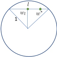
Figure 11: Graphic illustration about the sampling process in the proof of Theorem 22.

Proof  We just prove the theorem for $2n+m=d-1$. Note that this case can be simulated by considering an estimator with access to $2n+m$ truthful samples; that is, $Y_{i}=w^{*}\cdot X_{i}$ for $i=1,2,\ldots,2n+m$. In this way truthful comparisons can be simulated by query two labels. We now prove a lower bound for this new case with $2n+m=d-1$ truthful samples.

We randomly sample $w^{*}$ as below: first uniformly sample $v^{*}$ on the surface of $B(0,1)$, and then uniformly sample $r^{*}\in[0,1]$. Let this distribution be $\mathcal{P}_{w^{*}}$. Since we only have $d-1$ labels, for any set of samples $x_{1},\ldots,x_{d-1}$ there exists a line $l\in B(0,1)$ such that every $w\in l$ produces the same labels on all the samples. Not losing generality, suppose such $l$ is unique (if not, we can augment $\widehat{w}$ such that it always queries until $l$ is unique). Now for any active estimator $\widehat{w}$, let $X_{1},\ldots,X_{d-1}$ denote the sequence of queried points when $w^{*}$ is randomly picked as above. Now note that for every $w$,

$$\mathbb{P}[w^{*}=w|\{X_{i},y_{i}\}_{i=1}^{d-1},l]=\mathbb{P}[w^{*}=w|\{X_{i},y_{i}\}_{i=1}^{d-1}]\propto\mathbb{P}[w^{*}=w]I(w\in l).$$

The first equality is because $l$ is a function of $\{X_{i},y_{i}\}_{i=1}^{d-1}$; the second statement is because all $w\in l$ produces the same dataset on $X_{1},\ldots,X_{d-1}$, and every $w\not\in l$ is impossible given the dataset. Notice that $r^{*}$ is uniform on $[0,1]$; so with probability at least a half, the resulting $l$ has distance less than $1/2$ to the origin (since $l$ contains $w^{*}$, and $\|w^{*}\|$ is uniform on $[0,1]$). Denote by $w_{l}$ the middle point of $l$ (see Figure 11). For any such line $l$, the error is minimized by predicting the middle point of $l$: Actually we have

$$\mathbb{E}\left[\langle w^{*}-\widehat{w},\,X\rangle^{2}|\text{$l$ has distance less than 1/2}\right]\geq\int_{u=0}^{|l|/2}u^{2}dP(\|w^{*}-\widehat{w}\|_{2}\geq u|w^{*}\in l)$$ (23)

.

$$\geq\int_{u=0}^{|l|/2}u^{2}dP(\|w^{*}-w_{l}\|_{2}\geq u|w^{*}\in l)$$ (24)

Note that the distribution of $w^{*}\in l$ is equivalent to that we sample from the circle containing $l$ and centered at origin, and then condition on $w^{*}\in l$ (see Figure 11). Notice that this sampling process is the same as when $d=2$; and with some routine calculation we can show that (24) is a constant $C$. So overall we have

$$\mathbb{E}\left[\langle w^{*}-\widehat{w},\,X\rangle^{2}\right]\geq\frac{1}{2}C,$$

where the expectation is taken over randomness of $w^{*}$ and randomness of $\widehat{w}$. Now since the expectation is a constant, there must exists some $w$ such that

$$\mathbb{E}\left[\left.\langle w^{*}-\widehat{w},\,X\rangle^{2}\right|w^{*}=w\right]\geq\frac{1}{2}C,$$

which proves the theorem.  

C Auxiliary Technical Results

We use some well-known technical results in our proofs and collect them here to improve readability. We use the Craig-Bernstein inequality (Craig, 1933):

Lemma 23

Suppose we have $\{X_{1},\ldots,X_{n}\}$ be independent random variables and suppose that for $k\geq 2$, for some $r>0$,

$$\mathbb{E}[\left|X_{i}-\mathbb{E}[X_{i}]\right|^{k}]\leq\frac{\text{var}(X_{i})}{2}k!r^{k-2}.$$

Then with probability at least $1-\delta$, for any $c<1$ and for any $t\leq c/r$ we have that:

$$\frac{1}{n}\sum_{i=1}^{n}\left(\mathbb{E}[X_{i}]-X_{i}\right)\leq\frac{\log(1/\delta)}{nt}+\frac{t~{}\text{var}(X_{i})}{2(1-c)}.$$

References

- Agarwal et al. (2017) A. Agarwal, S. Agarwal, S. Assadi, and S. Khanna. Learning with limited rounds of adaptivity: Coin tossing, multi-armed bandits, and ranking from pairwise comparisons. In Conference on Learning Theory, pages 39–75, 2017.
- Agustsson et al. (2017) E. Agustsson, R. Timofte, S. Escalera, X. Baro, I. Guyon, and R. Rothe. Apparent and real age estimation in still images with deep residual regressors on appa-real database. In 12th IEEE International Conference and Workshops on Automatic Face and Gesture Recognition (FG), 2017. IEEE, 2017.
- Awasthi et al. (2014) P. Awasthi, M. F. Balcan, and P. M. Long. The power of localization for efficiently learning linear separators with noise. In Proceedings of the forty-sixth annual ACM symposium on Theory of computing, pages 449–458. ACM, 2014.
- Awasthi et al. (2016) P. Awasthi, M.-F. Balcan, N. Haghtalab, and H. Zhang. Learning and 1-bit compressed sensing under asymmetric noise. In Conference on Learning Theory, pages 152–192, 2016.
- Barlow (1972) R. Barlow. Statistical Inference Under Order Restrictions: The Theory and Application of Isotonic Regression. J. Wiley, 1972.
- Barron (1991) A. R. Barron. Complexity Regularization with Application to Artificial Neural Networks, chapter 7, pages 561–576. Springer Netherlands, 1991.
- Bellec (2018) P. C. Bellec. Sharp oracle inequalities for least squares estimators in shape restricted regression. The Annals of Statistics, 46(2):745–780, 2018.
- Bellec and Tsybakov (2015) P. C. Bellec and A. B. Tsybakov. Sharp oracle bounds for monotone and convex regression through aggregation. Journal of Machine Learning Research, 16:1879–1892, 2015.
- Bradley and Terry (1952) R. A. Bradley and M. E. Terry. Rank analysis of incomplete block designs: I. the method of paired comparisons. Biometrika, 39(3/4):324–345, 1952.
- Braverman and Mossel (2009) M. Braverman and E. Mossel. Sorting from noisy information. arXiv preprint arXiv:0910.1191, 2009.
- Castro and Nowak (2008) R. M. Castro and R. D. Nowak. Minimax bounds for active learning. IEEE Transactions on Information Theory, 54(5):2339–2353, 2008.
- Chatterjee et al. (2015) S. Chatterjee, A. Guntuboyina, and B. Sen. On risk bounds in isotonic and other shape restricted regression problems. Ann. Statist., 43(4):1774–1800, 08 2015.
- Chaudhuri and Dasgupta (2010) K. Chaudhuri and S. Dasgupta. Rates of convergence for the cluster tree. In Advances in Neural Information Processing Systems, pages 343–351, 2010.
- Chaudhuri et al. (2015) K. Chaudhuri, S. M. Kakade, P. Netrapalli, and S. Sanghavi. Convergence rates of active learning for maximum likelihood estimation. In Advances in Neural Information Processing Systems, pages 1090–1098, 2015.
- Craig (1933) C. C. Craig. On the Tchebychef inequality of Bernstein. The Annals of Mathematical Statistics, 4(2):94–102, 1933.
- Dasgupta and Luby (2017) S. Dasgupta and M. Luby. Learning from partial correction. arXiv preprint arXiv:1705.08076, 2017.
- Diaconis and Graham (1977) P. Diaconis and R. L. Graham. Spearman’s footrule as a measure of disarray. Journal of the Royal Statistical Society. Series B (Methodological), pages 262–268, 1977.
- Faber et al. (2016) F. A. Faber, A. Lindmaa, O. A. von Lilienfeld, and R. Armiento. Machine learning energies of 2 million Elpasolite(ABC2D6)crystals. Physical Review Letters, 117(13), 2016.
- Gilbert (1952) E. N. Gilbert. A comparison of signalling alphabets. Bell System Technical Journal, 31(3):504–522, 1952.
- Györfi et al. (2006) L. Györfi, M. Kohler, A. Krzyzak, and H. Walk. A distribution-free theory of nonparametric regression. Springer Science & Business Media, 2006.
- Han et al. (2017) Q. Han, T. Wang, S. Chatterjee, and R. J. Samworth. Isotonic regression in general dimensions. arXiv preprint arXiv:1708.09468, 2017.
- Hanneke (2009) S. Hanneke. Theoretical foundations of active learning. ProQuest, 2009.
- Härdle et al. (2012) W. K. Härdle, M. Müller, S. Sperlich, and A. Werwatz. Nonparametric and semiparametric models. Springer Science & Business Media, 2012.
- Joachims (2002) T. Joachims. Optimizing search engines using clickthrough data. In Proceedings of the eighth ACM SIGKDD international conference on Knowledge discovery and data mining, pages 133–142. ACM, 2002.
- Kane et al. (2017) D. M. Kane, S. Lovett, S. Moran, and J. Zhang. Active classification with comparison queries. arXiv preprint arXiv:1704.03564, 2017.
- Lovász and Vempala (2007) L. Lovász and S. Vempala. The geometry of logconcave functions and sampling algorithms. Random Structures & Algorithms, 30(3):307–358, 2007.
- Luce (2005) R. D. Luce. Individual choice behavior: A theoretical analysis. Courier Corporation, 2005.
- Plackett (1975) R. L. Plackett. The analysis of permutations. Applied Statistics, pages 193–202, 1975.
- Poulis and Dasgupta (2017) S. Poulis and S. Dasgupta. Learning with Feature Feedback: from Theory to Practice. In Proceedings of the 20th International Conference on Artificial Intelligence and Statistics, 2017.
- Ramaswamy et al. (2018) H. G. Ramaswamy, A. Tewari, S. Agarwal, et al. Consistent algorithms for multiclass classification with an abstain option. Electronic Journal of Statistics, 12(1):530–554, 2018.
- Schroff et al. (2015) F. Schroff, D. Kalenichenko, and J. Philbin. Facenet: A unified embedding for face recognition and clustering. In Proceedings of the IEEE conference on computer vision and pattern recognition, pages 815–823, 2015.
- Shah et al. (2016a) N. Shah, S. Balakrishnan, J. Bradley, A. Parekh, K. Ramchandran, and M. Wainwright. Estimation from pairwise comparisons: Sharp minimax bounds with topology dependence. Journal of Machine Learning Research, 2016a.
- Shah et al. (2016b) N. Shah, S. Balakrishnan, A. Guntuboyina, and M. Wainwright. Stochastically transitive models for pairwise comparisons: Statistical and computational issues. IEEE Transactions on Information Theory, 2016b.
- Shah et al. (2016c) N. B. Shah, S. Balakrishnan, and M. J. Wainwright. A permutation-based model for crowd labeling: Optimal estimation and robustness, 2016c.
- Thurstone (1927) L. L. Thurstone. A law of comparative judgment. Psychological review, 34(4):273, 1927.
- Tsukida and Gupta (2011) K. Tsukida and M. R. Gupta. How to analyze paired comparison data. Technical report, DTIC Document, 2011.
- Tsybakov (2004) A. B. Tsybakov. Optimal aggregation of classifiers in statistical learning. The Annals of Statistics, 32(1):135–166, 2004.
- Tsybakov (2009) A. B. Tsybakov. Introduction to nonparametric estimation. revised and extended from the 2004 french original. translated by vladimir zaiats, 2009.
- Varshamov (1957) R. Varshamov. Estimate of the number of signals in error correcting codes. In Dokl. Akad. Nauk SSSR, 1957.
- Willett et al. (2006) R. Willett, R. Nowak, and R. M. Castro. Faster rates in regression via active learning. In Advances in Neural Information Processing Systems, pages 179–186, 2006.
- Xu et al. (2017) Y. Xu, H. Zhang, K. Miller, A. Singh, and A. Dubrawski. Noise-tolerant interactive learning from pairwise comparisons with near-minimal label complexity. arXiv preprint arXiv:1704.05820, 2017.
- Xue et al. (2016) D. Xue, P. V. Balachandran, J. Hogden, J. Theiler, D. Xue, and T. Lookman. Accelerated search for materials with targeted properties by adaptive design. Nature Communications, 7, 2016.
- Yan and Zhang (2017) S. Yan and C. Zhang. Revisiting perceptron: Efficient and label-optimal learning of halfspaces. In Advances in Neural Information Processing Systems, pages 1056–1066, 2017.
- Zhang (2002) C.-H. Zhang. Risk bounds in isotonic regression. The Annals of Statistics, 30(2):528–555, 2002.
- Zou et al. (2015) J. Y. Zou, K. Chaudhuri, and A. T. Kalai. Crowdsourcing feature discovery via adaptively chosen comparisons. In Proceedings of the Third AAAI Conference on Human Computation and Crowdsourcing, HCOMP 2015, November 8-11, 2015, San Diego, California., page 198, 2015.