Applications of Gaussian Process Latent Variable Models in Finance

Abstract

Estimating covariances between financial assets plays an important role in risk management. In practice, when the sample size is small compared to the number of variables, the empirical estimate is known to be very unstable. Here, we propose a novel covariance estimator based on the Gaussian Process Latent Variable Model (GP-LVM). Our estimator can be considered as a non-linear extension of standard factor models with readily interpretable parameters reminiscent of market betas. Furthermore, our Bayesian treatment naturally shrinks the sample covariance matrix towards a more structured matrix given by the prior and thereby systematically reduces estimation errors. Finally, we discuss some financial applications of the GP-LVM.

1 Introduction

Many financial problems require the estimation of covariance matrices between given assets. This may be useful to optimize one’s portfolio, i.e.: maximize the portfolio returns $\bm{w}^{T}\bm{r}$ and/or minimize the volatility $\sqrt{\bm{w}^{T}\bm{K}\bm{w}}$. Indeed, Markowitz received a Noble Price in economics for his treatment of modern portfolio theory [1]. In practice, estimating historical returns and high-dimensional covariance matrices is challenging and often times equally weighted portfolio outperforms the portfolio constructed from sample estimates [2]. The estimation of covariance matrices is especially hard, when the number of assets is large compared to the number of observations. Sample estimations in those cases are very unstable or can even become singular. To cope with this problem, a wide range of estimators, e.g. factor models such as the single-index model [3] or shrinkage estimators [4], have been developed and employed in portfolio optimization.

With todays machine learning techniques we can even further improve those estimates. Machine learning has already arrived in finance. Nevmyvaka et al. [5] trained an agent via reinforcement learning to optimally execute trades. Gately [6] forecast asset prices with neural networks and Chapados et al. [7] with Gaussian Processes. Recently, Heaton et al. [8] made an ansatz to optimally allocate portfolios using deep autoencoders. Wu et al. [9] used Gaussian Processes to build volatility models and Wilson et al. [10] to estimate time varying covariance matrices. Bayesian machine learning methods are used more and more in this domain. The fact, that in a Bayesian framework parameters are not treated as true values, but as random variables, accounts for estimation uncertainties and can even alleviate the unwanted impacts of outliers. Furthermore, one can easily incorporate additional information and/or personal views by selecting suitable priors.

In this paper, we propose a Bayesian covariance estimator based on the Gaussian Process Latent Variable Models (GP-LVMs) [11], which can be considered as a non-linear extension of standard factor models with readily interpretable parameters reminiscent of market betas. Our Bayesian treatment naturally shrinks the sample covariance matrix (which maximizes the likelihood function) towards a more structured matrix given by the prior and thereby systematically reduces estimation errors. We evaluated our model on the stocks of S&P500 and found significant improvements in terms of model fit compared to classical linear models. Furthermore we suggest some financial applications, where Gaussian Processes can be used as well. That includes portfolio allocation, price prediction for less frequently traded stocks and non-linear clustering of stocks into their sub-sectors.

In section 2 we begin with an introduction to the Bayesian non-parametric Gaussian Processes and discuss the associated requirements for learning. Section 3 introduces the financial background needed for portfolio optimization and how to relate it to Gaussian Processes. In section 4 we conduct experiments on covariance matrix estimations and discuss the results. We conclude in section 5.

2 Background

In this paper, we utilize a Bayesian non-parametric machine learning approach based on Gaussian Processes (GPs). Combining those with latent variable models leads to Gaussian Process Latent Variable Models (GP-LVMs), that we use to estimate the covariance between different assets. These approaches have been described in detail in [11, 12]. We provide a brief review here. Subsequently, we show, how to relate those machine learning approaches to the known models in finance, e.g. the single-index model [3].

2.1 Gaussian Processes

A Gaussian Process (GP) is a generalization of the Gaussian distribution. Using a GP, we can define a distribution over functions $f(\bm{x})$, where $\bm{x}\in\mathbb{R}^{Q}$ and $f(\cdot)\in\mathbb{R}$. Like a Gaussian distribution, the GP is specified by a mean and a covariance. In the GP case, however, the mean is a function of the input variable $m(\bm{x})$ and the covariance is a function of two variables $k(\bm{x},\bm{x}^{\prime})$, which contains information about how the GP evaluated at $\bm{x}$ and $\bm{x}^{\prime}$ covary

$$m(\bm{x}) =\mathbb{E}[f(\bm{x})],$$ (1)

$$k(\bm{x},\bm{x}^{\prime}) =\text{cov}(f(\bm{x}),f(\bm{x}^{\prime})).$$ (2)

We write $f\sim\text{GP}(m(\cdot),k(\cdot,\cdot))$. Any finite collection of function values, at $\bm{x}_{1},\ldots,\bm{x}_{N}$, is jointly Gaussian distributed

$$p(f(\bm{x}_{1}),f(\bm{x}_{2}),...,f(\bm{x}_{N}))=\mathcal{N}(\bm{\mu},\bm{K}),$$ (3)

where $\bm{\mu}=(m(\bm{x}_{1}),...,m(\bm{x}_{N}))^{T}$ is the mean vector and $\bm{K}\in\mathbb{R}^{N\times N}$ is the Gram matrix with entries $\bm{K}_{ij}=k(\bm{x}_{i},\bm{x}_{j})$. We refer to the covariance function as kernel function. The properties of the function $f$ (i.e. smoothness, periodicity) are determined by the choice of this kernel function. For example, sampled functions from a GP with an exponentiated quadratic covariance function $k_{\text{SE}}(\bm{x},\bm{x}^{\prime})=\sigma^{2}\exp(-0.5||\bm{x}-\bm{x}^{\prime}||^{2}_{2}/l^{2})$ smoothly vary with lengthscale $l$ and are infinitely often differentiable.

Given a dataset $\mathcal{D}$ of $N$ input points $\bm{X}=(\bm{x_{1}},...,\bm{x_{N}})^{T}$ and $N$ corresponding targets $\bm{y}=(y_{1},...,y_{N})^{T}$, the predictive distribution for a zero mean GP at $N_{*}$ new locations $\bm{X}_{*}$ reads [12]

$$\bm{y}_{*}|\bm{X}_{*},\bm{y},\bm{X}\sim\mathcal{N}(\bm{f}_{*},\bm{K}_{*}),$$ (4)

where

$$\bm{f}_{*} =\bm{K}_{\bm{X}_{*}\bm{X}}\bm{K}_{\bm{XX}}^{-1}\bm{y},$$ (5)

$$\bm{K}_{*} =\bm{K}_{\bm{X}_{*}\bm{X}_{*}}-\bm{K}_{\bm{X}_{*}\bm{X}}\bm{K}_{\bm{XX}}^{-1}\bm{K}_{\bm{X}\bm{X}_{*}}.$$ (6)

$\bm{K}_{\bm{X}_{*}\bm{X}}\in\mathbb{R}^{N_{*}\times N}$ is the covariance matrix between the GP evaluated at $\bm{X}_{*}$ and $\bm{X}$, $\bm{K}_{\bm{XX}}\in\mathbb{R}^{N\times N}$ is the covariance matrix of the GP evaluated at $\bm{X}$. As we can see in equations (5) and (6), the kernel function plays a very important role in the GP framework and will be important for our financial model as well.

2.2 Gaussian Process Latent Variable Model

Often times we are just given a data matrix $\bm{Y}\in\mathbb{R}^{N\times D}$ and the goal is to find a lower dimensional representation $\bm{X}\in\mathbb{R}^{N\times Q}$, without losing too much information. Principal component analysis (PCA) is one of the most used techniques for reducing the dimensions of the data, which has also been motivated as the maximum likelihood solution to a particular form of Gaussian Latent Variable Model [13]. PCA embeds $\bm{Y}$ via a linear mapping into the latent space $\bm{X}$. Lawrence [11] introduced the Gaussian Process Latent Variable Model (GP-LVM) as a non-linear extension of probabilistic PCA. The generative procedure takes the form

$${\bm{Y}}_{{n},:}=\bm{f}({\bm{X}}_{{n},:})+\bm{\epsilon}_{n},$$ (7)

where $\bm{f}=(f_{1},...,f_{D})^{T}$ is a group of $D$ independent samples from a GP, i.e. $f_{d}\sim\text{GP}(0,k(\cdot,\cdot))$. By this, we assume the rows of $\bm{Y}$ to be jointly Gaussian distributed and the columns to be independent, i.e. each sample ${\bm{Y}}_{:,{d}}\sim\mathcal{N}({\bm{Y}}_{:,{d}}|\bm{0},\bm{K})$ where $\bm{K}=k(\bm{X},\bm{X})+\sigma^{2}\mathbf{I}$ and $\sigma^{2}$ denotes the variance of the random noise $\bm{\epsilon}$. The marginal likelihood of $\bm{Y}$ becomes [11]

$$p(\bm{Y}|\bm{X})=\prod_{d=1}^{D}\mathcal{N}({\bm{Y}}_{:,{d}}|\bm{0},\bm{K})=\frac{1}{(2\pi)^{ND/2}|\bm{K}|^{D/2}}\exp\left(-\frac{1}{2}\text{tr}(\bm{K}^{-1}\bm{YY}^{T})\right).$$ (8)

The dependency on the latent positions $\bm{X}$ and the kernel hyperparameters is given through the kernel matrix $\bm{K}$. As suggested by Lawrence [11], we can optimize the log marginal likelihood $\log p(\bm{Y}|\bm{X})$ with respect to the latent positions and the hyperparameters.

2.3 Variational Inference

Optimization can easily lead to overfitting. Therefore, a fully Bayesian treatment of the model would be preferable but is intractable. Bishop [14] explains the variational inference framework, which not only handles the problem of overfitting but also allows to automatically select the dimensionality of the latent space. Instead of optimizing equation (8), we want to calculate the posterior using Bayes rule $p(\bm{X}|\bm{Y})=p(\bm{Y}|\bm{X})p(\bm{X})/p(\bm{Y})$, which is intractable. The idea behind variational Bayes is to approximate the true posterior $p(\bm{X}|\bm{Y})$ by another distribution $q(\bm{X})$, selected from a tractable family. The goal is to select the one distribution $q(\bm{X})$, that is closest to the true posterior $p(\bm{X}|\bm{Y})$ in some sense. A natural choice to quantify the closeness is given by the Kullback-Leibler divergence [15]

$$\text{KL}[q(\bm{X})||p(\bm{X}|\bm{Y})]=\int q(\bm{X})\log\frac{q(\bm{X})}{p(\bm{X}|\bm{Y})}\mathrm{d}\bm{X}.$$ (9)

By defining $\tilde{p}(\bm{X}|\bm{Y})=p(\bm{Y}|\bm{X})p(\bm{X})$ as the unnormalized posterior, equation (9) becomes

$$\text{KL}[q(\bm{X})||p(\bm{X}|\bm{Y})] =\int q(\bm{X})\log\frac{q(\bm{X})}{\tilde{p}(\bm{X}|\bm{Y})}\mathrm{d}\bm{X}+\log p(\bm{Y})$$

$$=-\underbrace{\mathbb{E}_{q(\bm{X})}\left[\log\frac{\tilde{p}(\bm{X}|\bm{Y})}{q(\bm{X})}\right]}_{\text{ELBO}}+\log p(\bm{Y})$$ (10)

with the first term on the right hand side being known as the evidence lower bound (ELBO). Equation (10) is the objective function we want to minimize with respect to $q(\bm{X})$ to get a good approximation to the true posterior. Note that on the left hand side only the ELBO is $q$ dependent. So, in order to minimize (10), we can just as well maximize the ELBO. Because the Kullback-Leibler divergence is non-negative, the ELBO is a lower bound on the evidence $\log p(\bm{Y})$. Therefore, this procedure not only gives the best approximation to the posterior within the variational family under the KL ceriterion, but it also bounds the evidence, which serves as a measure of the goodness of our fit. The number of latent dimensions $Q$ can be chosen to be the one, which maximizes the ELBO.

So, GP-LVM is a model, which reduces the dimensions of our data-matrix $\bm{Y}\in\mathbb{R}^{N\times D}$ from $D$ to $Q$ in a non-linear way and at the same time estimates the covariance matrix between the $N$ points. The estimated covariance matrix can then be used for further analysis.

3 Finance

Now we have a procedure to estimate the covariance matrix between different datapoints. This section discusses how we can relate this to financial models.

3.1 CAPM

The Capital Asset Pricing Model (CAPM) describes the relationship between the expected returns of an asset $\bm{r}_{n}\in\mathbb{R}^{D}$ for D days and its risk $\beta_{n}$

$$\mathbb{E}[\bm{r}_{n}]=\bm{r}_{f}+\beta_{n}\mathbb{E}[\bm{r}_{m}-\bm{r}_{f}],$$ (11)

where $\bm{r}_{f}\in\mathbb{R}^{D}$ is the risk free return on $D$ different days and $\bm{r}_{m}$ is the market return on D different days. The main idea behind CAPM is, that an investor needs to be compensated for the risk of his holdings. For a risk free asset with $\beta_{n}=0$, the expected return $\mathbb{E}[\bm{r}_{n}]$ is just the risk free rate $\bm{r}_{f}$. If an asset is risky with a risk $\beta_{n}\neq 0$, the expected return $\mathbb{E}[\bm{r}_{n}]$ is increased by $\beta_{n}\mathbb{E}[\tilde{\bm{r}}_{m}]$, where $\tilde{\bm{r}}_{m}$ is the excess return of the market $\tilde{\bm{r}}_{m}=\bm{r}_{m}-\bm{r}_{f}$.

We can write down equation (11) in terms of the excess return $\tilde{\bm{r}}=\bm{r}-\bm{r}_{f}$ and get

$$\mathbb{E}[\tilde{\bm{r}}_{n}]=\beta_{n}\mathbb{E}[\tilde{\bm{r}}_{m}],$$ (12)

where $\tilde{\bm{r}}_{n}$ is the excess return of a given asset and $\tilde{\bm{r}}_{m}$ is the excess return of the market (also called a risk factor). Arbitrage pricing theory [16] generalizes the above model by allowing multiple risk factors $\bm{F}$ beside the market $\tilde{\bm{r}}_{m}$. In particular, it assumes that asset returns follow a factor structure

$$\bm{r}_{n}=\alpha_{n}+\bm{F}\bm{\beta}_{n}+\bm{\epsilon}_{n},$$ (13)

with $\bm{\epsilon}_{n}$ denoting some independent zero mean noise with variance $\sigma^{2}_{n}$. Here, $\bm{F}\in\mathbb{R}^{D\times Q}$ is the matrix of Q factor returns on D days and $\bm{\beta}_{n}\in\mathbb{R}^{Q}$ is the loading of stock $n$ to the Q factors. Arbitrage pricing theory [17] then shows that the expected excess returns adhere to

$$\mathbb{E}[\tilde{\bm{r}}_{n}]=\mathbb{E}[\tilde{\bm{F}}]\bm{\beta}_{n},$$ (14)

i.e. the CAPM is derived as special case when assuming a single risk factor (single-index model).

To match the form of the GP-LVM (see equation (7)), we rewrite equation (13) as

$${\bm{r}}_{{n},:}=\bm{f}({\bm{B}}_{{n},:})+\bm{\epsilon}_{n},$$ (15)

where $\bm{r}\in\mathbb{R}^{N\times D}$ is the return matrix. Note that assuming latent factors distributed as $\bm{F}\sim\mathcal{N}(0,1)$ and marginalizing over them, equation (13) is a special case of equation (15) with $\bm{f}$ drawn from a GP mapping $\bm{\beta}_{n}$ to $\bm{r}_{n}$ with a linear kernel. Interestingly, this provides an exact correspondence with factor models by considering the matrix of couplings $\bm{B}=(\bm{\beta_{1}},...,\bm{\beta_{N}})^{T}$ as the latent space positions. In this perspective the factor model can be seen as a linear dimensionality reduction, where we reduce the $N\times D$ matrix $\bm{r}$ to a low rank matrix $\bm{B}$ of size $N\times Q$. By chosing a non-linear kernel $k(\cdot,\cdot)$ the GP-LVM formulation readily allows for non-linear dimensionality reductions. Since, it is generally known, that different assets have different volatilities, we further generalize the model. In particular, we assume the noise $\bm{\epsilon}$ to be a zero mean Gaussian, but allow for different variances $\sigma^{2}_{n}$ for different stocks. For this reason, we also have to parameterize the kernel (covariance) matrix in a different way than usual. Section 4.1 explains how to deal with that. The model is then approximated using variational inference as described in section 2.3. After inferring $\bm{B}$ and the hyperparameters of the kernel, we can calculate the covariance matrix $\bm{K}$ and use it for further analysis.

3.2 Modern Portfolio Theory

Markowitz [1] provided the foundation for modern portfolio theory, for which he received a Nobel Prize in economics. The method analyses how good a given portfolio is, based on the mean and the variance of the returns of the assets contained in the portfolio. This can also be formulated as an optimization problem for selecting an optimal portfolio, given the covariance between the assets and the risk tolerance $q$ of the investor.

Given the covariance matrix $\bm{K}\in\mathbb{R}^{N\times N}$, we can calculate the optimal portfolio weights $\bm{w}$ by

$$\bm{w}_{\text{opt}}=\min_{\bm{w}}(\bm{w}^{T}\bm{K}\bm{w}-q\bar{\bm{r}}^{T}\bm{w}),$$ (16)

where $\bar{\bm{r}}$ is the mean return vector. Risk friendly investors have a higher $q$ than risk averse investors. The model is constrained by $\sum_{\bm{w}}=1$. Since $\bar{\bm{r}}$ is very hard to estimate in general and we are primarily interested in the estimation of the covariance matrix $\bm{K}$, we set $q$ to zero and get

$$\bm{w}_{\text{opt}}=\min_{\bm{w}}(\bm{w}^{T}\bm{K}\bm{w}).$$ (17)

This portfolio is called the minimal risk portfolio, i.e. the solution to equation (17) provides the weights for the portfolio, which minimizes the overall risk, assuming the estimated $\bm{K}$ is the true covariance matrix.

4 Experiments

In this section, we discuss the performance of the GP-LVM on financial data. After describing the data collection and modeling procedure, we evaluate the model on the daily return series of the S&P500 stocks. Subsequently, we discuss further financial applications. In particular, we show how to build a minimal risk portfolio (this can easily be extended to maximizing returns as well), how to fill-in prices for assets which are not traded frequently and how to visualize sector relations between different stocks (latent space embedding).

4.1 Data Collection and Modeling

For a given time period, we take all the stocks from the S&P500, whose daily close prices were available for the whole period. The data were downloaded from Yahoo Finance. After having the close prices in a matrix $\bm{p}\in\mathbb{R}^{N\times(D+1)}$, we calculate the return matrix $\bm{r}\in\mathbb{R}^{N\times D}$, where $\bm{r}_{nd}=(\bm{p}_{n,d}-\bm{p}_{n,d-1})/\bm{p}_{n,d-1}$. $\bm{r}$ builds the basis of our analysis.

We can feed $\bm{r}$ into the GP-LVM. The GP-LVM procedure, as described in section 2, assumes the likelihood to be Gaussian with the covariance given by the kernel function for each day and assumes independency over different days. We use the following kernel functions

$$k_{\text{noise}}(\bm{\beta}_{i},\bm{\beta}_{j})=\sigma_{\text{noise},i}^{2}\delta_{i,j},$$

$$k_{\text{linear}}(\bm{\beta}_{i},\bm{\beta}_{j})=\sigma^{2}\bm{\beta}_{i}^{T}\bm{\beta}_{j},$$ (18)

and the stationary kernels

$$k_{\text{se}}(\bm{\beta}_{i},\bm{\beta}_{j})=k_{\text{se}}(d_{ij})=\exp\left(-\frac{1}{2l^{2}}d_{ij}^{2}\right),$$

$$k_{\text{exp}}(\bm{\beta}_{i},\bm{\beta}_{j})=k_{\text{exp}}(d_{ij})=\exp\left(-\frac{1}{2l}d_{ij}\right),$$

$$k_{\text{m32}}(\bm{\beta}_{i},\bm{\beta}_{j})=k_{\text{m32}}(d_{ij})=\left(1+\frac{\sqrt{3}d_{ij}}{l}\right)\exp\left(-\frac{\sqrt{3}}{2l}d_{ij}\right),$$ (19)

where $d_{ij}=||\bm{\beta}_{i}-\bm{\beta}_{j}||_{2}$ is the Euclidean distance between $\bm{\beta}_{i}$ and $\bm{\beta}_{j}$. $\sigma^{2}$ is the kernel variance and $l$ kernel lengthscale. Note that since the diagonal elements of stationary kernels are the same, they are not well suited for an estimation of a covariance matrix between different financial assets. Therefore, in the case of stationary kernel we decompose our covariance matrix $\bm{K}_{\text{cov}}$ into a vector of coefficient scales $\bm{\sigma}$ and a correlation matrix $\bm{K}_{\text{corr}}$, such that $\bm{K}_{\text{cov}}=\bm{\Sigma}\bm{K}_{\text{corr}}\bm{\Sigma}$, where $\bm{\Sigma}$ is a diagonal matrix with $\bm{\sigma}$ on the diagonal. The full kernel function $k(\cdot,\cdot)$ at the end is the sum of the noise kernel $k_{\text{noise}}$ and one of the other kernels. In matrix form we get

$$\bm{K}_{\text{linear}}=k_{\text{linear}}(\bm{B},\bm{B})+k_{\text{noise}}(\bm{B},\bm{B}),$$

$$\bm{K}_{\text{se}}=\bm{\Sigma}\ k_{\text{se}}(\bm{B},\bm{B})\ \bm{\Sigma}+k_{\text{noise}}(\bm{B},\bm{B}),$$

$$\bm{K}_{\text{exp}}=\bm{\Sigma}\ k_{\text{exp}}(\bm{B},\bm{B})\ \bm{\Sigma}+k_{\text{noise}}(\bm{B},\bm{B}),$$

$$\bm{K}_{\text{m32}}=\bm{\Sigma}\ k_{\text{m32}}(\bm{B},\bm{B})\ \bm{\Sigma}+k_{\text{noise}}(\bm{B},\bm{B}),$$ (20)

where $\bm{B}=(\bm{\beta}_{1},...,\bm{\beta}_{N})^{T}$. We chose the following priors

$$\bm{B}\sim\mathcal{N}(0,1)\qquad\quad l,\sigma\sim\text{InvGamma}(3,1)\qquad\quad\bm{\sigma},\sigma_{noise}\sim\mathcal{N}(0,0.5).$$ (21)

The prior on $\bm{B}$ determines how much space is allocated to the points in the latent space. The volume of this space expands with higher latent space dimension, which make the model prone to overfitting. To cope with that, we assign an inverse gamma prior to the lengthscale $l$ and $\sigma$ ($\sigma$ in the linear kernel has a similar functionality as $l$ in the stationary kernels). It allows larger values for higher latent space dimension, thereby shrinking the effective latent space volume and exponentially suppresses very small values, which deters overfitting as well. The parameters of the priors are chosen such that they allow for enough volume in the latent space for roughly 100-150 datapoints, which we use in our analysis. If the number of points is drastically different, one should adjust the parameters accordingly. The kernel standard deviations $\sigma_{\text{noise}}$ and $\bm{\sigma}$ are assigned a half Gaussian prior with variance 0.5, which is essentially a flat prior, since the returns are rarely above 0.1 for a day.

Model inference under these specifications (GP-LVM likelihood for the data and prior for $\bm{B}$ and all kernel hyperparameters $\sigma,\sigma_{\text{noise}},l$ and $\bm{\sigma}$, which we denote by $\bm{\theta}$) was carried out by variational inference as described in section 2.3. To this end, we implemented all models in the probabilistic programming language Stan [18], which supports variational inference out of the box. We approximate the posterior by independent Gaussians. The source code is available on Github. We tested different initializations for the parameter (random, PCA solution and Isomap solution), but there were no significant differences in the ELBO. So, we started the inference 50 times with random initializations and took the result with highest ELBO for each kernel function and $Q$.

4.2 Model Comparison

The GP-LVM can be evaluated in many different ways. Since, it projects the data from a $D$-dimensional space to a $Q$-dimensional latent space, we can look at the reconstruction error. A suitable measure of the reconstruction error is the R-squared ($R^{2}$) score, which is equal to one if there is no reconstruction error and decreases if the reconstruction error increases. It is defined by

$$R^{2}=1-\frac{\sum_{i}(y_{i}-f_{i})^{2}}{\sum_{i}(y_{i}-\bar{y})^{2}},$$ (22)

where $y=(y_{1},...,y_{N})^{T}$ are the true values, $f=(f_{1},...f_{N})^{T}$ are the predicted values and $\bar{y}$ is the mean of $y$. In the following, we look at the $R^{2}$ as a function of the latent dimension $Q$ for different kernels. Figure 1 (left plot) shows the results for three non-linear kernels and the linear kernel. Only a single dimension in the non-linear case can already capture almost 50% of the structure, whereas the linear kernel is at 15%. As one would expect, the higher $Q$, the more structure can be learned. But at some point the model will also start learning the noise and overfit.

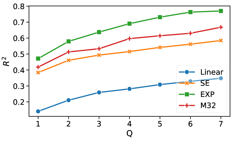
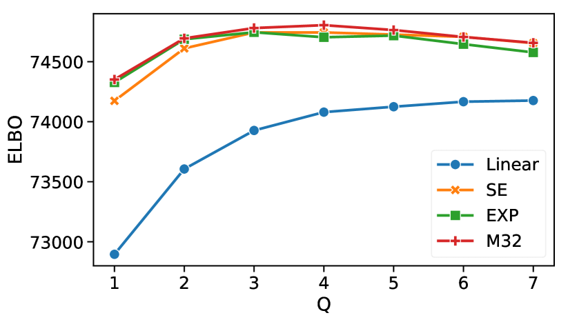
Figure 1: Left: $R^{2}$-score as a function of the latent dimension $Q$ for different kernel functions. Right: ELBO as a function of the latent dimension $Q$. We randomly chose 120 stocks from the S&P500 and made the analysis on returns from Jan 2017 to Dec 2017.

As introduced in section 2.3, the ELBO is a good measure to evaluate different models and already incorporates models complexity (overfitting). Figure 1 (right plot) shows the ELBO as a function of the latent dimension $Q$. Here we see, that the model selects just a few latent dimensions. Depending on the used kernel, latent dimensions from three to five are already enough to capture the structure. If we increase the dimensions further, the ELBO starts dropping, which is a sign of overfitting. As can be seen from Figure 1, we do not need to go to higher dimensions. $Q$ between two and five is already good enough and captures the structure that can be captured by the model.

4.3 Applications

The GP-LVM provides us the covariance matrix $\bm{K}$ and the latent space representation $\bm{B}$ of the data. We can build a lot of nice applications upon that, some of which are discussed in this section.

4.3.1 Portfolio Allocation

After inferring $\bm{B}$ and $\bm{\theta}$, we can reconstruct the covariance matrix $\bm{K}$ using equation (20). Thereafter, we only need to minimize equation (17), which provides the weights $\bm{w}$ for our portfolio in the future. Minimization of (17) is done under the constraints: $\sum_{n}\bm{w}_{n}=1$ and $0<\bm{w}_{n}<0.1,\forall n$. These constraints are commonly employed in practice and ensure that we are fully invested, take on long positions only and prohibit too much weight for a single asset.

For our tests, we proceed as follows: First, we get data for 60 randomly selected stocks from the S&P500 from Jan 2008 to Jan 2018. Then, we learn $\bm{w}$ from the past year and buy accordingly for the next six months. Starting from Jan 2008, this procedure is repeated every six months. We calculate the average return, standard deviation and the Sharpe ratio. [19] suggested the Sharpe ratio as a measure for a portfolio‘s performance, which is the average return earned per unit of volatility and can be calculated by dividing the mean return of a series by its standard deviation. Table 1 shows the performance of the portfolio for different kernels for $Q=3$. For the GP-LVM we chose the linear, SE, EXP and M32 kernels and included the performance given by the sample covariance matrix, i.e. $\bm{K}=\frac{1}{D}(\bm{r}-\hat{\bm{\mu}})(\bm{r}-\hat{\bm{\mu}})^{T}$, where $\hat{\bm{\mu}}_{n}=\frac{1}{D}\sum_{d=1}^{D}\bm{r}_{nd}$, the shrunk Ledoit-Wolf covariance matrix [4] and the equally weighted portfolio, where $\bm{w}=(1,1,...,1)/N$.

Table 1: Mean returns, standard deviation and the Sharpe ratio of different models on a yearly basis.

Model	Linear	SE	EXP	M32	Sample Cov	Ledoit Wolf	Eq. Weighted
Mean	0.142	0.151	0.155	0.158	0.149	0.148	0.182
Std	0.158	0.156	0.154	0.153	0.159	0.159	0.232
Sharpe ratio	0.901	0.969	1.008	1.029	0.934	0.931	0.786

Non-linear kernels have the minimal variance and at the same time the best Sharpe ratio values. Note that we are building a minimal variance portfolio and therefore not maximizing the mean returns as explained in section 3.2. For finite $q$ in equation (16) one can also build portfolios, which not only minimize risk but also maximize the returns. Another requirement for that would be to have a good estimator for the expected return as well.

4.3.2 Fill in Missing Values

Regulation requires fair value assessment of all assets [21], including illiquid and infrequently traded ones. Here, we demonstrate how the GP-LVM could be used to fill-in missing prices, e.g. if no trading took place. For illustration purposes, we continue working with our daily close prices of stocks from the S&P500, but the procedure can be applied to any other asset class and time resolution.

First, we split our data $\bm{r}$ into training and test set. The test set contains days where the returns of assets are missing and our goal is to accurately predict the return. In our case, we use stock data from Jan 2017 to Oct 2017 for training and Nov 2017 to Dez 2017 to test. The latent space $\bm{B}$ and the hyperparameters $\bm{\theta}$ are learned from the training set. Given $\bm{B}$ and $\bm{\theta}$, we can use the standard GP equations (eq. (5) and (6)) to get the posterior return distribution. A suggestion for the value of the return at a particular day can be made by the mean of this distribution. Given $N$ stocks for a particular day $d$, we fit a GP to $N-1$ stocks and predict the value of the remaining stock. We repeat the process $N$ times, each time leaving out a different stock (Leave-one-out cross-validation). Figure 2 shows the $R^{2}$-score (eq. (22)) and the average absolute deviation $\frac{1}{ND}\sum_{nd}|\bm{r}_{nd}-\bm{r}^{\text{pred}}_{nd}|$ of the suggested return to the real return. The average is build over all stocks and all days in the test set.

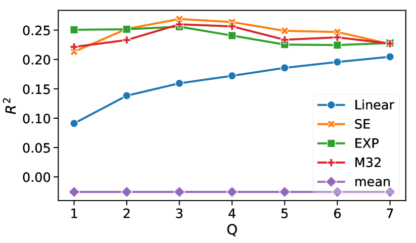
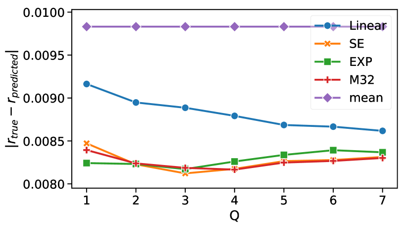
Figure 2: Left: $R^{2}$-score of the predicted values as a function of the latent dimension $Q$. Right: The average absolute deviation of suggested return to the real return evaluated by Leaving-one-out cross-validation. Historical mean is indicated by “mean” and is Q-independent.

The predictions with just the historical mean have a negative $R^{2}$-score. The linear model is better than that. But if we switch to non-linear kernels, we can even further increase the prediction score. For $Q$ between 2 and 4 we obtain the best results. Note that to make a decent suggestion for the return of an asset, there must be some correlated assets in the data as well. Otherwise, the model has no information at all about the asset, we want to predict the returns for.

4.3.3 Interpretation of the Latent Space

The 2-dimensional latent space can be visualized as a scatter plot. For a stationary kernel function like the SE, the distance between the stocks is directly related to their correlation. In this case, the latent positions are even easier to interpret than market betas. As an example, Figure 3 shows the 2-D latent space from 60 randomly selected stocks from the S&P500 from Jan 2017 to Dec 2017. Visually stocks from the same sector tend to cluster together and we consider our method as an alternative to other methods for detecting structure in financial data [22].

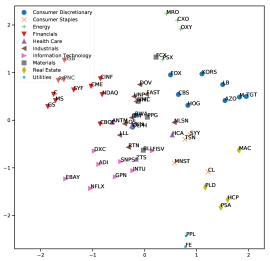
Figure 3: Stocks visualised in the 2-D latent space for the SE kernel.

5 Conclusion

We applied the Gaussian Process Latent Variable Model (GP-LVM) to estimate the covariance matrix between different assets, given their time series. We then showed how the GP-LVM can be seen as a non-linear extension to the CAPM with latent factors. Based on the $R^{2}$-score and the ELBO, we concluded, that for fixed latent space dimension $Q$, every non-linear kernel can capture more structure than the linear one.

The estimated covariance matrix helps us to build a minimal risk portfolio according to Markowitz Portfolio theory. We evaluated the performance of different models on the S&P500 from year 2008 to 2018. Again, non-linear kernels had lower risk in the suggested portfolio and higher Sharpe ratios than the linear kernel and the baseline measures. Furthermore, we showed how to use the GP-LVM to fill in missing prices of less frequently traded assets and we discussed the role of the latent positions of the assets. In the future, one could also put a Gaussian Process on the latent positions and allow them to vary in time, which would lead to a time-dependent covariance matrix.

Acknowledgments

The authors thank Dr. h.c. Maucher for funding their positions.

References

- [1] Harry Markowitz. Portfolio selection. The Journal of Finance, 7(1):77–91, 1952.
- [2] J. D. Jobson and Robert M Korkie. Putting markowitz theory to work. The Journal of Portfolio Management, 7(4):70–74, 1981.
- [3] William F. Sharpe. Capital asset prices with and without negative holdings. The Journal of Finance, 46(2):489–509, 1991.
- [4] Olivier Ledoit and Michael Wolf. Honey, I shrunk the sample covariance matrix. The Journal of Portfolio Management, 30(4):110–119, 2004.
- [5] Yuriy Nevmyvaka, Yi Feng, and Michael Kearns. Reinforcement learning for optimized trade execution. In Proceedings of the 23rd International Conference on Machine Learning, ICML ’06, pages 673–680, New York, NY, USA, 2006. ACM.
- [6] Edward Gately. Neural Networks for Financial Forecasting. John Wiley & Sons, Inc., New York, NY, USA, 1995.
- [7] Nicolas Chapados and Yoshua Bengio. Augmented functional time series representation and forecasting with gaussian processes. In J. C. Platt, D. Koller, Y. Singer, and S. T. Roweis, editors, Advances in Neural Information Processing Systems 20, pages 265–272. Curran Associates, Inc., 2008.
- [8] J. B. Heaton, N. G. Polson, and J. H. Witte. Deep Portfolio Theory. Papers 1605.07230, arXiv.org, May 2016.
- [9] Yue Wu, José Miguel Hernández-Lobato, and Zoubin Ghahramani. Gaussian process volatility model. In Z. Ghahramani, M. Welling, C. Cortes, N. D. Lawrence, and K. Q. Weinberger, editors, Advances in Neural Information Processing Systems 27, pages 1044–1052. Curran Associates, Inc., 2014.
- [10] Andrew Gordon Wilson and Zoubin Ghahramani. Generalised wishart processes. In Proceedings of the Twenty-Seventh Conference on Uncertainty in Artificial Intelligence, UAI’11, pages 736–744, Arlington, Virginia, United States, 2011. AUAI Press.
- [11] Neil Lawrence. Probabilistic non-linear principal component analysis with gaussian process latent variable models. J. Mach. Learn. Res., 6:1783–1816, December 2005.
- [12] Carl Edward Rasmussen. Gaussian processes for machine learning. MIT Press, 2006.
- [13] Michael E. Tipping and Chris M. Bishop. Probabilistic principal component analysis. Journal of the Royal Statistical Society, Series B, 61:611–622, 1999.
- [14] Christopher M. Bishop. Pattern Recognition and Machine Learning (Information Science and Statistics). Springer-Verlag, Berlin, Heidelberg, 2006.
- [15] Thomas M. Cover and Joy A. Thomas. Elements of Information Theory. Wiley-Interscience, New York, NY, USA, 1991.
- [16] Richard Roll and Stephen Ross. The arbitrage pricing theory approach to strategic portfolio planning. Financial Analysts Journal, 51:122–131, Jan 1995.
- [17] Stephen A Ross. The arbitrage theory of capital asset pricing. Journal of Economic Theory, 13(3):341 – 360, 1976.
- [18] Bob Carpenter, Andrew Gelman, Matthew Hoffman, Daniel Lee, Ben Goodrich, Michael Betancourt, Marcus Brubaker, Jiqiang Guo, Peter Li, and Allen Riddell. Stan: A probabilistic programming language. Journal of Statistical Software, Articles, 76(1):1–32, 2017.
- [19] William F. Sharpe. Mutual fund performance. The Journal of Business, 39(1):119–138, 1966.
- [20] F. Pedregosa, G. Varoquaux, A. Gramfort, V. Michel, B. Thirion, O. Grisel, M. Blondel, P. Prettenhofer, R. Weiss, V. Dubourg, J. Vanderplas, A. Passos, D. Cournapeau, M. Brucher, M. Perrot, and E. Duchesnay. Scikit-learn: Machine learning in Python. Journal of Machine Learning Research, 12:2825–2830, 2011.
- [21] Financial Accounting Standards Board. Statement of financial accounting standards no. 157 – fair value measurements, 2006. Norwalk, CT.
- [22] Michele Tumminello, Fabrizio Lillo, and Rosario N. Mantegna. Correlation, hierarchies, and networks in financial markets. Journal of Economic Behavior & Organization, 75:40–58, 2010.