A Physically Constrained Inversion for Super-resolved Passive Microwave Retrieval of Soil Moisture and Vegetation Water Content in L-band

Abstract

Remote sensing of soil moisture and vegetation water content from space often requires underdetermined inversion of a zeroth-order approximation of the forward radiative transfer equation in L-band, known as the $\tau$-$\omega$ model. This paper shows that the least-squares inversion of the model is not strictly convex and the widely used unconstrained damped least-squares (DLS) can lead to biased retrievals, chiefly due to the existing preferential solution spaces that are characterized by the eigenspace of the model’s Hessian. In particular, the numerical experiments show that for sparse (dense) vegetation with a shallow (deep) optical depth, the DLS tends to overestimate (underestimate) the soil moisture and vegetation water content for a dry (wet) soil. A new Constrained Multi-Channel Algorithm (CMCA) is proposed that bounds the retrievals with a priori information about the soil type and vegetation density and can account for slowly varying dynamics of the vegetation water content over croplands through a temporal smoothing-norm regularization in the derivative domain. It is demonstrated that depending on the resolution of the constraints, the algorithm can lead to super-resolved soil moisture retrievals beyond the spatial resolution of radiometric observations. Multiple Monte Carlo retrieval experiments are conducted and the results are validated against ground-based gauge observations.

1 Introduction

Soil moisture is only less than 5 percent of the Earth’s freshwater reservoirs [1] but plays a key role in regulating the water mass transport and energy exchange in the soil-plant-atmosphere continuum. The Earth’s vegetation, and thus the global food security, depends on the soil moisture climatology [2]. Trends in intensity, frequency and duration of the global precipitation [3], resulting from a changing climate, makes monitoring of soil moisture a key factor to extend forecast skill of land-atmosphere models [4, 5]; improve drought modeling and management [6, 7]; and further unravel processes that regulate evapotranspiration [8, 9], as well as carbon [10] and nitrogen cycles [11].

Emission of surface soil in microwave frequencies between 1 to 5 GHz is sensitive to soil moisture content. The upwelling electromagnetic waves penetrate well through the overlaying canopy with moderate water content (i.e., $<$ 5 kg m^-2) and reach to the top of the atmosphere with negligible interactions with the atmospheric constituents [12]. The L-band (1-2 GHz) radiometry has been central to soil moisture satellite missions [13, 14] including the NASA’s Soil Moisture Active Passive (SMAP, [15]) satellite.

In L-band, the surface soil emission and its interaction with vegetation biomass can be represented well through a zeroth-order nonlinear approximation of the radiative transfer equation [16, 17, 18, 12, and references there in]—known as the $\tau$-$\omega$ model. This forward model relates the surface temperature to the observed brightness temperatures at the top of the atmosphere as a function of rough surface soil reflectivity, vegetation transmissivity and single scattering albedo. Thus, inversion of this model could lead to the retrievals of not only the soil moisture but also the vegetation water content (VWC) [e.g., 19, 20, 21, 22]. Both of the soil reflectivity and vegetation transmissivity are polarization dependent; however, evidence suggests that the polarization dependence of the former is more pronounced than the latter in L-band. The single scattering albedo is the least dynamic parameter of the model and is often considered polarization independent and seasonally invariant [23, 24, 25].

Simultaneous retrieval of the soil moisture and the vegetation transmissivity from single L-band radiometry could lead to an ill-posed nonlinear inverse problem. To make the problem well-posed, a priori information can be provided in different ways. In particular, there are two major classes of inversion algorithms—namely single channel (SCA) and dual channel (DCA) algorithms. The SCA only uses horizontal or vertical polarization of the observed brightness temperatures [26]. To make the inversion well-posed, prior information is supplied through ancillary data. In particular, it is assumed that the single scattering albedo is a known constant over different land covers and the vegetation transmissivity can be estimated off-line from climatology of the normalized difference vegetation index (NDVI).

The DCA uses both polarization channels to compute the unknown parameters simultaneously, through a nonlinear least-squares (LS) inversion [21]. Due to the strong dependence of the observed brightness temperatures at different polarization channels, this inversion is often ill-conditioned, especially for the SMAP single band radiometer. To make the inversion possible, the DCA often relies on the Levenberg-Marquardt (LM) or the damped least-squares (DLS) optimization algorithm [27, 28]. This iterative algorithm can find a minimum solution of an ill-posed nonlinear LS problem using an adaptive Tikhonov regularization [29].

Other advanced DCA inversion approaches have also been proposed that rely on the DLS. Piles et al. [30] recast the retrieval as an overdetermined inverse problem by proposing to use the first guess of the free parameters as a-priori knowledge, assuming that the uncertainties follow a Gaussian distribution. More recently, Konings et al. [31] adopted a time series approach that retrieves the real component of the soil dielectric constant within a window of time—over which, it is assumed that the vegetation optical depth remains constant. A review of existing algorithms can be found in the SMAP handbook [32] and also in [33].

The contribution of this paper can be summarized as follows. First, we show that the LS inversion of the $\tau$-$\omega$ model is not strictly convex, which leads to a preferential solution space and biased DCA retrievals. Second, we propose to use a Tikhonov regularization to add box constraints to an LS inversion of the model that will lead to the retrievals that are physically consistent with the soil moisture capacity and climatology of vegetation phenology. Third, we extend the existing time-series retrieval algorithms [31] to account for the slow-varying changes in the vegetation water content, through a smoothing-norm regularization in a derivative domain. Fourth, we provide initial results that the algorithm can lead to higher resolution retrievals of soil moisture and vegetation water content than the native resolution of the SMAP radiometer, depending on the resolution of the constraints.

Section 2 presents introductory materials about the forward $\tau$-$\omega$ model and provides conceptual details about its LS inversion. This section sets the stage for discussing the convexity of the inversion (Section 2.1) and reasoning about potential biases in the DLS retrievals (Section 2.2). Section 3 proposes the new multi-frequency inversion formalism. Through Monte Carlo simulations, we demonstrate in Section 4.1 that this new approach leads to almost unbiased retrievals with reduced uncertainty compared to classic unconstrained DLS retrievals. In Section 4.2, we extend the inversion formalism for retrievals over a window of time. Section 4.3 discusses implementation of the algorithm for a super-resolved soil moisture retrieval using SMAP data and some initial validation results are presented in Section 4.4. Section 5 provides discussions, concludes and points out to future directions and the need for a thorough ground validation of the algorithm.

2 A review of the $\tau$-$\omega$ Model and its Least-squares Inversion

The $\tau$-$\omega$ model has been explained in numerous seminal publications [e.g., 17, 34, 12]. Here, we briefly discuss the model to set the stage for investigating its convexity and potential biases that may arise in its LS inversion.

The $\tau$-$\omega$ model treats the vegetation layer as a weakly scattering medium with a low single scattering albedo, typically less than 0.2 in frequencies from 1 to 5 GHz. The model has three components: (1) emission by the soil surface $(1-r_{p})\gamma_{p}T_{s}$, (2) upward emission by the slanted column of vegetation with a finite thickness $(1-\omega_{p})(1-\gamma_{p})T_{c}$, and (3) canopy downward emission followed by soil coherent reflection $r_{p}(1-\omega_{p})(1-\gamma_{p})\gamma_{p}T_{c}$. Therefore, the observed brightness $Tb_{p}$ can be expressed as follows:

$$Tb_{p}=(1-r_{pr})\gamma_{p}T_{s}+(1-\omega_{p})(1-\gamma_{p})T_{c}+r_{pr}(1-\omega_{p})(1-\gamma_{p})\gamma_{p}T_{c},$$ (1)

where $T_{s}$ and $T_{c}$ are the effective soil surface and canopy thermodynamic temperatures, $r_{pr}$ denotes the rough surface soil coherent reflectivity, $\gamma_{p}$ is the canopy one-way transmissivity, and $\omega_{p}$ refers to the vegetation single scattering albedo. Here, the subscript $p\in\left\{H,\,V\right\}$ denotes that the quantity can be horizontally (H) or vertically (V) polarized.

To make this inversion well-posed, the family of single channel algorithms (SCA) assumes that the $\omega_{p}$ is a known constant for different land surface types and the vegetation transmissivity is approximately unpolarized and can be estimated from the NDVI climatology [35]. This approach assumes that the vegetation optical depth $\tau$ is linearly related to the vegetation water content (VWC) as $\tau=b\,.\text{VWC}$, where $b$ typically varies between 0.05 to 6.0 m² kg ^-1, depending on the vegetation type [36]. The algorithm estimates the VWC from 10-day climatology of NDVI through some regression equations [35, 37, 38] and a-prior knowledge of the plant’s stem structure [39, 40]. Having the optical depth, the vegetation transmissivity can be calculated as $\gamma=\text{exp}\left(-\tau\,\sec\phi\right)$, where $\phi$ denotes the radiometer incident angle in radians. Then, the smooth surface soil reflectivity value $r_{p}$ is derived from their rough counterpart $r_{pr}$ using $r_{pr}=r_{p}\exp\left(-h\,\cos\phi\right)$, where $h$ is linearly related to the root-mean-squared variability of the surface height [41]. Finally, the soil moisture is estimated using the Fresnel equations and a soil dielectric model [e.g., 42, 43, 44]. As is evident, the SCA does not retrieve the vegetation parameters and can not capture short-term changes in VWC, which could be an important source of error over grass and croplands. For example, the field campaign Soil Moisture Experiment 2002 (SMEX02) shows that in a growing season, the VWC can increase from $\sim 0.75$ to 2 km m^-2 every 10 days in a corn field [22].

The class of dual channel algorithms (DCA) [21] often relies on nonlinear LS inversion of the $\tau$-$\omega$ model using the DLS optimization algorithm. To be more specific, let us assume that in equation (1) the microwave surface emissivity at polarization $p$ is $e_{p}=Tb_{p}/T_{s}=f(\theta_{p})+\epsilon$, where the canopy and soil temperature are assumed to be at equilibrium $T_{s}=T_{c}$, $\theta_{p}=(r_{pr},\,\gamma_{p},\,\omega_{p})^{T}$, and $\epsilon$ denotes an error term that can be approximated well by the Gaussian distribution. Then, the LS retrieval can be defined as follows:

$$\theta_{p}^{*} =\underset{\theta_{p}}{\text{argmin}}\,\mathcal{J}(\theta_{p})$$

$$=\underset{\theta_{p}}{\text{argmin}}\frac{1}{2}\left(e_{p}-f(\theta_{p})\right)^{2}.$$ (2)

Hereafter, we drop the polarization subscript for notational convenience.

The DLS optimization is a Newton-type algorithm that attempts to construct a sequence $\theta_{k+1}=\theta_{k}+\delta_{k}$ from an initial guess $\theta_{0}$ that converges to $\theta^{*}$, where $\delta_{k}$ denotes the search direction. In classic Newton’s method, the search direction is obtained by minimizing the following quadratic approximation of the cost function at each iteration:

$$\mathcal{Q}(\delta_{k})=\mathcal{J}(\theta_{k})+\delta_{k}^{T}\,g_{k}+\frac{1}{2}\delta_{k}^{T}H_{k}\delta_{k},$$ (3)

where $g_{k}\stackrel{{\scriptstyle\text{def}}}{{=}}\nabla\mathcal{J}\left(\theta_{k}\right)$ and $H_{k}$ is a symmetric approximation of the Hessian matrix $\nabla^{2}\mathcal{J}\left(\theta_{k}\right)$ at $k^{\text{th}}$ step. Thus, the search direction can be obtained by solving $H_{k}\delta_{k}=-g_{k}$ for $\delta_{k}$. This linear system of equations is underdetermined for inversion of the $\tau$-$\omega$ model for the SMAP single band radiometer.

The classic DLS algorithm approximates the Hessian as $H_{k}\simeq g_{k}\,g_{k}^{T}$ and solves a damped version of the linear system such that $\left(H_{k}+\lambda_{k}I\right)\delta_{k}=-g_{k}$, where the damping parameter $\lambda_{k}$ is selected adaptively. Thus, the DLS algorithm uses a Tikhonov regularization to solve for the search direction, which makes the problem well-posed, even if the system is underdetermined. Spectral decomposition of $H_{k}=Q_{k}\Lambda_{k}Q_{k}^{T}$ to its eigenvectors in column space of $Q_{k}$ and eigenvalues as diagonals of $\Lambda_{k}$ leads to $Q_{k}\left(\Lambda_{k}+\lambda_{k}I\right)Q_{k}^{T}\,\delta_{k}=-g_{k}$. We can see that the search direction depends not only on the gradient of the cost function but also on the direction and magnitude of the eigenvectors of the Hessian. This observation prompts us to pose the following key questions. Is the LS inversion of the $\tau$-$\omega$ model a convex problem? Are the solutions of the DLS algorithm physically consistent?

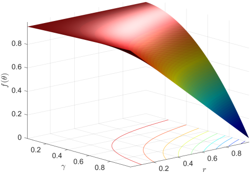
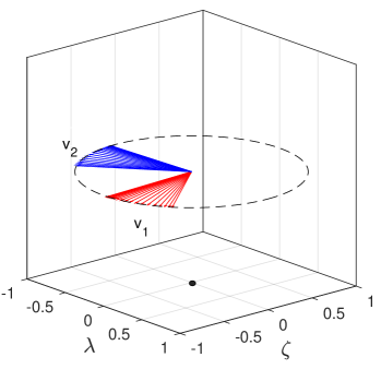
Figure 1: The $\tau$-$\omega$ model shows a saddle point behavior (left) for which the eigenvectors with positive ($\mathbf{v}_{1}$) and negative ($\mathbf{v}_{2}$) eigenvalues (right) characterize the directions of convexity and concavity of the model. The eigenvalues are calculated for rough soil surface reflectivity ranging from 0.4 to 1 and a vegetation optical depth that varies from 0.01 to 3 m.

2.1 Convexity of Inversion

The representation of the $\tau$-$\omega$ model through $f(\theta)$ is shown in Figure 1 for $\omega=0.05$. By visual inspection, we can see that the model does not produce a strictly convex or concave surface. In effect, assuming that $\omega$ is a constant, the Hessian is

$$H^{f}=\left[\begin{array}[]{cc}f_{\gamma\gamma}&f_{\gamma r}\\ f_{r\gamma}&f_{rr}\end{array}\right]=\left[\begin{array}[]{cc}2r\left(\omega-1\right)&\zeta\\ \zeta&0\end{array}\right],$$ (4)

where $\zeta=\gamma\left(\omega-1\right)+(\gamma-1)(\omega-1)-1$. Thus, the Hessian is a saddle point indefinite matrix with one positive ($\lambda_{1}$) and one negative ($\lambda_{2}$) eigenvalue such that $\lambda_{1,\,2}=r(\omega-1)\pm\sqrt{r^{2}\left(\omega-1\right)^{2}+\zeta^{2}}$ with the corresponding eigenvectors $\mathbf{v}_{1,\,2}=\left(\lambda_{1,\,2},\,\zeta\right)^{T}$. These eigenvectors determine two orthogonal directions along which the model shows convexity and concavity (Figure 1). Since $r(\omega-1)<0$, we have $\left|\lambda_{2}\right|\geq\left|\lambda_{1}\right|$ and thus the model is more concave than convex. Assuming that $\omega$ is constant, without loss of generality, we have

$$\mathcal{J}_{rr}=\frac{\partial^{2}\mathcal{J}}{\partial r^{2}}=\left[\gamma+\gamma(\gamma-1)\left(\omega-1\right)\right]^{2}>0.$$ (5)

Therefore, for characterizing the sub-region over which the problem is convex, it suffices to check where $\det\left(H^{\mathcal{J}}\right)=\mathcal{J}_{rr}\,\mathcal{J}_{\gamma\gamma}-\left(\mathcal{J}_{r\gamma}\right)^{2}$ is non-negative (Figure 2). Thus, underdetermined inversion of the $\tau$-$\omega$ model is not strictly convex all over the feasible domain of the problem. However, due to monotonic behavior of the model, the LS cost function exhibits quasi-convexity [45, p. 98]. Due to this non-convexity, the gradient-based approaches such as the DLS algorithm may not converge to the solution curve for those initial points that are outside of the convex domain of the problem.

   

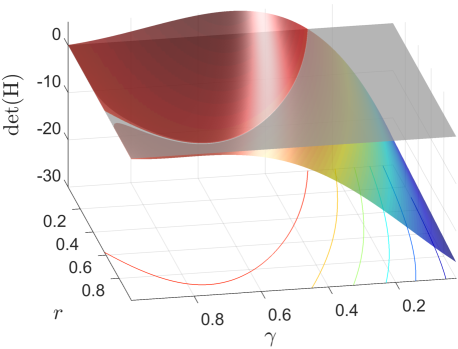
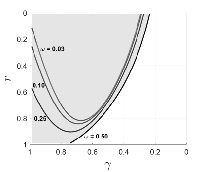
Figure 2: Delineating the convex sub-domain of the LS inversion of the $\tau$-$\omega$ model. The shown are the determinant of the Hessian of the LS cost function in problem 2 for $\omega=0.05$ (left) and the shaded regions over which the Hessian is positive semidefinite (right).

2.2 Physical Consistency of the Inversion

As discussed, the search direction of the DLS retrievals could follow preferential paths depending on the direction of the gradient and eigenvalues of the Hessian. The question is –how do these preferential search paths affect the solution space and physical consistency of the soil moisture retrievals? To answer this question, we conducted Monte Carlo retrieval experiments for two different scenarios. First, we conduced the retrievals for a few values of microwave surface emissivity ranging from 0.3 to 0.95, while the initial soil reflectivity and vegetation transmissivity are randomly drawn between 0 and 1 from a uniform distribution. Second, the input microwave emissivity values are also randomized by drawing samples from a uniform distribution between 0 and 1. To run the DLS in both cases, we consider $\lambda_{0}=0.01$ and $\lambda_{k+1}=0.1\,\lambda_{k}$, when the search direction reduces the cost function, otherwise $\lambda_{k+1}=10\,\lambda_{k}$. The density scatter plot of both experiments are shown in Figure 3.

      

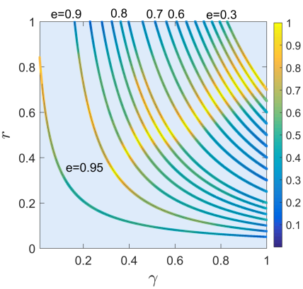
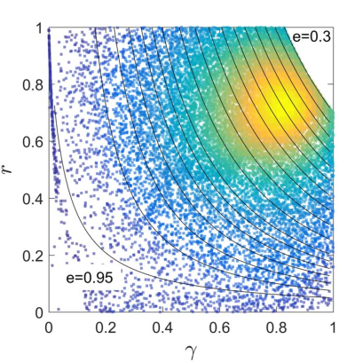
Figure 3: The density of retrievals showing preferential convergence pathways of the DLS solutions. The density of the retrievals is obtained through $2.5$e+4 random simulations, uniformly distributed over a few level sets (left) and the entire feasible space of the soil surface reflectivity and vegetation transmissivity values (right). The non-uniform distribution of solutions demonstrates that the simultaneous retrievals could systematically overestimate (underestimate) the soil moisture and VWC when the soil is dry (wet) under a sparse (dense) vegetation.

The results reveal a non-uniform solution space for the DLS algorithm. The retrievals are mostly concentrated on the upper right corner of the feasible solution space and mostly around the mid-point of the level sets. Concentration of the retrievals near the upper corner of the plot is not surprising because the feasible solution curves are shorter for higher values of $r$ and $\gamma$ and thus a discrete approximation of the solution space should be denser over that region. However, concentration of the solutions around the mid-point of the level sets shows the effects of preferential descending paths, which can lead to biased and physically inconsistent retrievals.

Overall, it seems that for sparse (dense) vegetation with a shallow (deep) optical depth, the DLS tends to underestimate (overestimate) the transmissivity and overestimate (underestimate) the surface reflectivity, which results in overestimation (underestimation) of both soil moisture and VWC. This pattern of biased retrievals is more pronounced when the microwave emissivity is below 0.9. For dry soil with higher microwave emissivity, it appears that the retrievals tend to systematically overestimate both of the variables.

3 Constrained Inversion of the $\tau$-$\omega$ Model

The systematic biases could be reduced by constraining the solution space using an a priori knowledge about the feasible range of the soil moisture and VWC [46]. In reality, the soil moisture and VWC are not unbounded physical parameters. In any retrieval scene, the soil moisture is bounded by soil porosity and often varies between the the permanent wilting (PWP) point and natural saturation. The VWC and its temporal dynamics also largely depend on the plants physiology and phenology. To avoid retrieval biases, we suggest the following constrained retrieval approach:

$$\theta^{*}=\underset{\theta}{\text{argmin}}\frac{1}{2}\left(e-f(\theta)\right)^{2}\,\,\,\,\text{subject to}\,\,\,\,\theta_{l}\preceq\theta\preceq\theta_{u},$$ (6)

where $\theta_{l}=(r_{l},\,\gamma_{l})^{T}$, $\preceq$ is an element-wise inequality and $\theta_{u}=(r_{u},\,\gamma_{u})^{T}$ denotes the lower and upper bounds of the input parameters. This problem is not tractable unless we provide additional a priori knowledge that turns it into an (over)determined problem.

The class of constrained nonlinear LS problems is often solved by a family of optimization techniques called the Trust Region (TR) algorithms [47, 48]. In this method the search direction at each iterate is obtained by minimizing a quadratic approximation of the objective function over a restricted ellipsoidal region centered on the current iterate. Therefore, at each step, the algorithm solves a constrained quadratic sub-problem, which makes it computationally more burdensome than the DLS approach. However, this construction prevents overshooting the local minima and thus could improve the convergence rate. The constrained sub-problem can be further equipped with computationally cheap projection operators to map the solution, at each iterate $\theta_{k+1}=\theta_{k}+\delta_{k}$, onto the convex set of $\theta_{l}\preceq\theta_{k}\preceq\theta_{u}$ [49].

To recast the inversion to an overdetermined problem, we suggest to add a Tikhonov regularization as follows:

$$\theta^{*}=\underset{\theta}{\text{argmin}\,}\left(e-f(\theta)\right)^{2}+\lambda\left\|\theta\right\|_{2}^{2}\,\,\,\,\text{subject to}\,\,\,\,\theta_{l}\preceq\theta\preceq\theta_{u}.$$ (7)

where $\lambda>0$ is a non-negative parameter and $\left\|\theta\right\|_{2}^{2}$ is the 2-norm or sum of the squares of the unknownparameters. The above problem can be recast to a standard form as follows:

$$\theta^{*}=\underset{\theta}{\text{argmin}}\,\left\|\left(\begin{array}[]{c}e-f(\theta)\\ \lambda^{1/2}\theta\end{array}\right)\right\|_{2}^{2}\,\,\,\,\text{subject to}\,\,\,\,\theta_{l}\preceq\theta\preceq\theta_{u}.$$ (8)

For ill-posed linear inverse problems, it is well documented that the Tikhonov regularization leads to a unique solution with reduced uncertainty. This reduced uncertainty often comes at the expense of a bias in the solution [50] that can be negligible for sufficiently small values of $\lambda$. Figure 4 shows the level sets of the cost function in problem 8 for $\lambda=0$ and 0.015, when $\omega=0.05$. When $\lambda\rightarrow 0$ , the problem approaches to the classic LS inversion with infinite number of solutions. For positive values of $\lambda$, a convex region is formed, which narrows down the solution space and reduces the retrieval uncertainties.

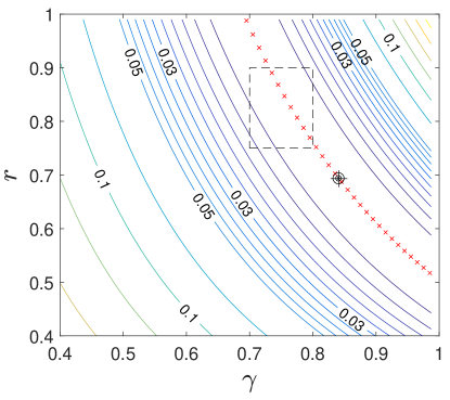
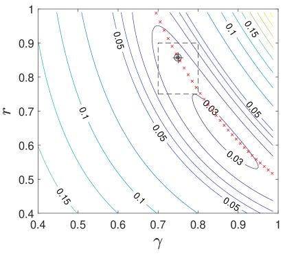
Figure 4: The level sets of the cost function in problem 8 for inversion of the $\tau$-$\omega$ model, with $\lambda=0.0$ (left) and $\lambda=0.015$ (right), in which $T_{s}=298$ K, $Tb=148$ K, and $\omega=0.05$. The solution curve for $\lambda=0$ is shown with red crosses. The black concentric circles with the plus sign at the center show the solution of unconstrained (left, equation 2) and constrained retrievals (right, equation 8). The constrained retrieval is obtained assuming that $\gamma\in\left[0.70\,0.80\right]$ and $r\in\left[0.75\,0.90\right]$—shown by a rectangle with dashed sides.

To expand the above inversion to a multi-channel algorithm, let us assume that $\mathbf{e}=\left(e_{1},\ldots,e_{q}\right)^{T}\in\mathbb{R}^{q}$ and $\boldsymbol{\theta}=\left(\theta_{1},\ldots,\theta_{q}\right)^{T}\in\mathbb{R}^{nq}$ denote the microwave emissivity and input parameters at $q$ frequencies, where $\theta_{q}\in\mathbb{R}^{1\times n}$ denotes a column vector with $n$ unknown free parameters. In addition, one may want to consider a $q$-by-$q$ error covariance $\mathbf{E}\in\mathbb{R}^{q\times q}$ to account for the precision of each channel. In this setting a multi-channel formulation of the above inversion scheme can be represented in the following standard form:

$$\boldsymbol{\theta}^{*}=\underset{\boldsymbol{\theta}}{\text{argmin}}\,\left\|\left(\begin{array}[]{c}\mathbf{E}^{-1/2}\left(\mathbf{e}-f(\boldsymbol{\theta})\right)\\ \lambda^{1/2}\boldsymbol{\theta}\end{array}\right)\right\|_{2}^{2}\,\,\,\,\text{subject to}\,\,\,\,\boldsymbol{\theta}_{l}\preceq\boldsymbol{\theta}\preceq\boldsymbol{\theta}_{u},$$ (9)

where $f(\boldsymbol{\theta}):\,\mathbb{R}^{nq}\rightarrow\mathbb{R}^{q}$ and there are $(n+1)q$ equations and $nq$ unknowns.

Additionally, extension to the retrievals over a window of time can be recast as follows:

$$\boldsymbol{\theta}_{\tau}^{*}=\underset{\boldsymbol{\theta}_{\tau}}{\text{argmin}}\left\|\left(\begin{array}[]{c}\mathbf{\mathbf{E}}_{\tau}^{-1/2}\left(\mathbf{e}_{\tau}-f(\boldsymbol{\theta}_{\tau})\right)\\ \Lambda^{1/2}\mathbf{D}\boldsymbol{\theta}_{\tau}\end{array}\right)\right\|_{2}^{2}\,\,\,\,\text{subject to}\,\,\,\,\boldsymbol{\theta}_{l\tau}\preceq\boldsymbol{\theta}_{\tau}\preceq\boldsymbol{\theta}_{u\tau},$$ (10)

where $f(\boldsymbol{\theta}_{\tau}):\,\mathbb{R}^{nqt}\rightarrow\mathbb{R}^{qt}$ , $\mathbf{e}_{\tau}=\left(\mathbf{e}_{1}^{T},\ldots,\mathbf{e}_{t}^{T}\right)^{T}\in\mathbb{R}^{qt}$ and $\boldsymbol{\theta}_{\tau}=\left(\mathbf{\boldsymbol{\theta}}_{1}^{T},\ldots,\mathbf{\boldsymbol{\theta}}_{t}^{T}\right)^{T}\in\mathbb{R}^{nqt}$ stack all the observed microwave emissivity values and free parameters in a vector form over a window of time with size $\tau=1,\ldots,t$. Here, $\mathfrak{\mathbf{E}}_{\tau}\in\mathbb{R}^{qt\times qt}$ is a block diagonal matrix in which, each block contains the channel error covariance matrix $\mathbf{E}\in\mathbb{R}^{q\times q}$ and $\mathbf{D}\in\mathbb{R}^{m\times nqt}$ ($m\leq nqt$) is a linear transformation that can impose an a priori information about the temporal variability of the free parameters. For example, instead of assuming that the vegetation water content remains constant over a window of time, one may assume that it is a slow varying process. One way to formalize this assumption is to impose a certain degree of smoothness by minimizing the variance of a temporal derivative of the vegetation transmissivity. As a result, to properly scale the problem, we might need different regularization parameters for the soil reflectivity and vegetation transmissivity, which are encoded by the diagonal matrix $\Lambda=\textrm{diag}\left(\lambda_{1},\ldots,\lambda_{m}\right)\in\mathbb{R}^{m\times m}$. Hereafter, we refer to the presented approach as the Constrained Multi-Channel Algorithm (CMCA).

4 Implementation, Results and Validation

In this section, we implement and validate the performance of the CMCA algorithm in three steps. In the first step, we examine the results using a Monte Carlo approach to compare the CMCA performance with unconstrained DLS inversion and evaluate its results under fully controlled boundary conditions. In the second step, we use soil moisture gauge data to evaluate the results of the CMCA algorithm for retrievals over a window of time. In the third step, we implement the algorithmic for the SMAP satellite observations and validate it against soil moisture gauge observations.

4.1 A Monte Carlo Validation

For conducting a controlled validation, we adopt a Monte Carlo approach. To that end, we generate a statistically representative number of random combinations of physically feasible free input parameters and simulate their brightness temperatures using the forward $\tau$-$\omega$ model at 1.4 GHz and incident angle 40^∘. These brightness temperatures are then used for retrievals of the known free parameters. In the experiments, we assume that the rough surface soil reflectivity values are polarization dependent while vegetation transmissivity is not.

Throughout, to confine the computational domain, we assume that $\omega=0.05$, the constant that relates VWC to its optical depth $b=0.10$, and the soil surface roughness parameter $h=0.12$ [see 41]. To understand the effects of vegetation density and soil types on the accuracy of retrievals, we conduct our experiments separately for three ranges of VWC between 0 and 1.5, 1.5 and 3.0, and 3.0 and 5.0 kg m^-2. The simulations are also stratified based on the National Resources Conservation Service (NRCS) soil texture classification. In the experiments, we assume that the soil moisture varies between the permanent wilting point (suction head -1500 kPa) and the field capacity (suction head -33 kPa). The bounds of the rough soil surface reflectivity values for the NRCS soil types are reported in Table 1.

Texture	PWP (%)	FC(%)	Clay content	$r_{Hr\ell}$	$r_{Hru}$	$r_{Vr\ell}$	$r_{Vru}$
Clay	30.0	42.0	40.0-100	0.27	0.50	0.11	0.30
Silty clay	27.0	41.0	40.0-60.0	0.32	0.48	0.15	0.30
Silty clay loam	22.0	38.0	27.5-40.0	0.32	0.48	0.15	0.30
Clay loam	22.0	36.0	27.5-40.0	0.32	0.48	0.15	0.30
Silt	6.00	30.0	0.00-12.5	0.16	0.45	0.05	0.27
Silt loam	11.0	31.0	0.00-27.5	0.20	0.46	0.07	0.28
Sandy clay	25.0	36.0	35.00-55.0	0.31	0.46	0.15	0.28
Loam	14.0	28.0	7.50-27.50	0.25	0.43	0.10	0.25
Sandy clay loam	17.0	27.0	20.0-35.0	0.27	0.40	0.11	0.23
Sandy loam	8.00	18.0	0.00-20.0	0.18	0.35	0.06	0.18
Loamy sand	5.00	12.0	0.00-15.0	0.15	0.28	0.04	0.12
Sand	5.00	10.0	0.00-10.0	0.16	0.25	0.04	0.10
All soil types	-	-	-	0.15	0.50	0.04	0.30

Table 1: The lower and upper bounds of the soil moisture and the rough soil surface reflectivity values at horizontal ($r_{Hr}$) and vertical polarization ($r_{Vr}$) for different NRCS soil types at incident angle 40^∘ and $f=1.4$ GHz, using the soil dielectric model by Mironov et al. [43]. The values of the permanent wilting point (PWP) and the field capacity (FC) are obtained from [51].

In Table 1, silt and sand show the widest and narrowest range of surface soil surface reflectivity, respectively—largely because of the range of their water capacity. It is important to note that, based on the chosen dielectric model, the variability range of $r_{Hr}$ is $\sim 50$% larger than its vertical counterpart—when the real part of the soil dielectric constant varies between 0 and 20. Generally speaking, a wider range of surface reflectivity may imply more sensitivity of the channel to the changes of soil moisture content. However, provided that the bounds are physically consistent, a narrower bound is a stronger prior, which could lead to reduced retrieval uncertainties. Certainly, this argument shall be interpreted independent of the observation noise and accuracy of the radiometer at different polarization channels.

To evaluate the result of the CMCA, we first need to determine an optimal value of the regularization parameter $\lambda$ in equation 8, for which there is no closed form expression.

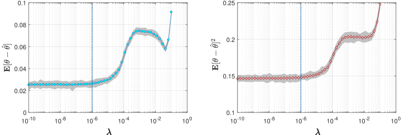
Figure 5: The bias (left) and the RMSE (right) of the CMCA retrievals for 60 retrieval ensembles (shaded region) as a function of the regularization parameter $\lambda$ ranging from 1e-10 to 1, where $\theta=\left(r_{Hr},\,r_{Vr},\,\gamma\right)^{T}$.

Figure 5 shows the bias and root mean squared error (RMSE) of CMCA retrievals as a function of $\lambda$, where $\theta=\left(r_{rH},\,r_{rV},\,\gamma\right)^{T}$. The shaded region shows the upper and lower bounds of 60 ensemble simulations. Specifically, we generated 2.5e+3 uniformly distributed random inputs of surface temperature 0–40^∘, soil moisture 0.05–0.42, VWC 0–5.0 kg m^-2, and soil clay content 0–99%. Based on these input parameters, we ran the $\tau$-$\omega$ model and corrupted the simulated brightness temperatures with a zero-mean white Gaussian noise with standard deviation 1.3 K to resemble the observed brightness temperatures by the SMAP radiometer. Then, the bias and RMSE of the CMCA retrievals are obtained as a function of $\lambda$. We repeated this process for 60 times to evaluate the sensitivity of the retrievals to the observation noise. As is evident, for $\lambda$ values $\leq$ 1e-6, the bias and RMSE are minimum and the solutions are fairly stable. Above this threshold the the quality metrics begin to grow rapidly. As the $\lambda$ becomes larger, the shaded areas begin to gradually shrink, which means the observation noise is further suppressed and the solutions become more stable. However, we can see that the bias is also growing.

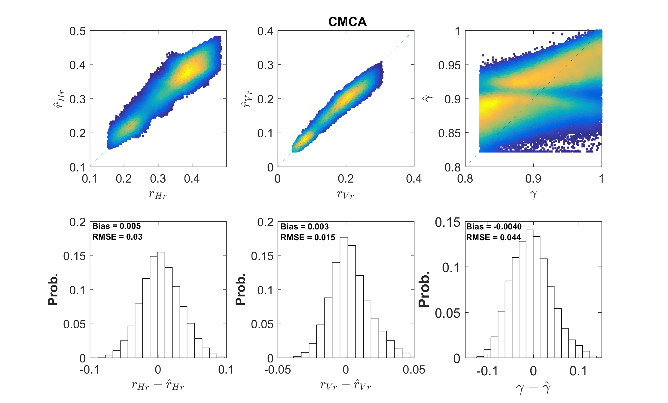
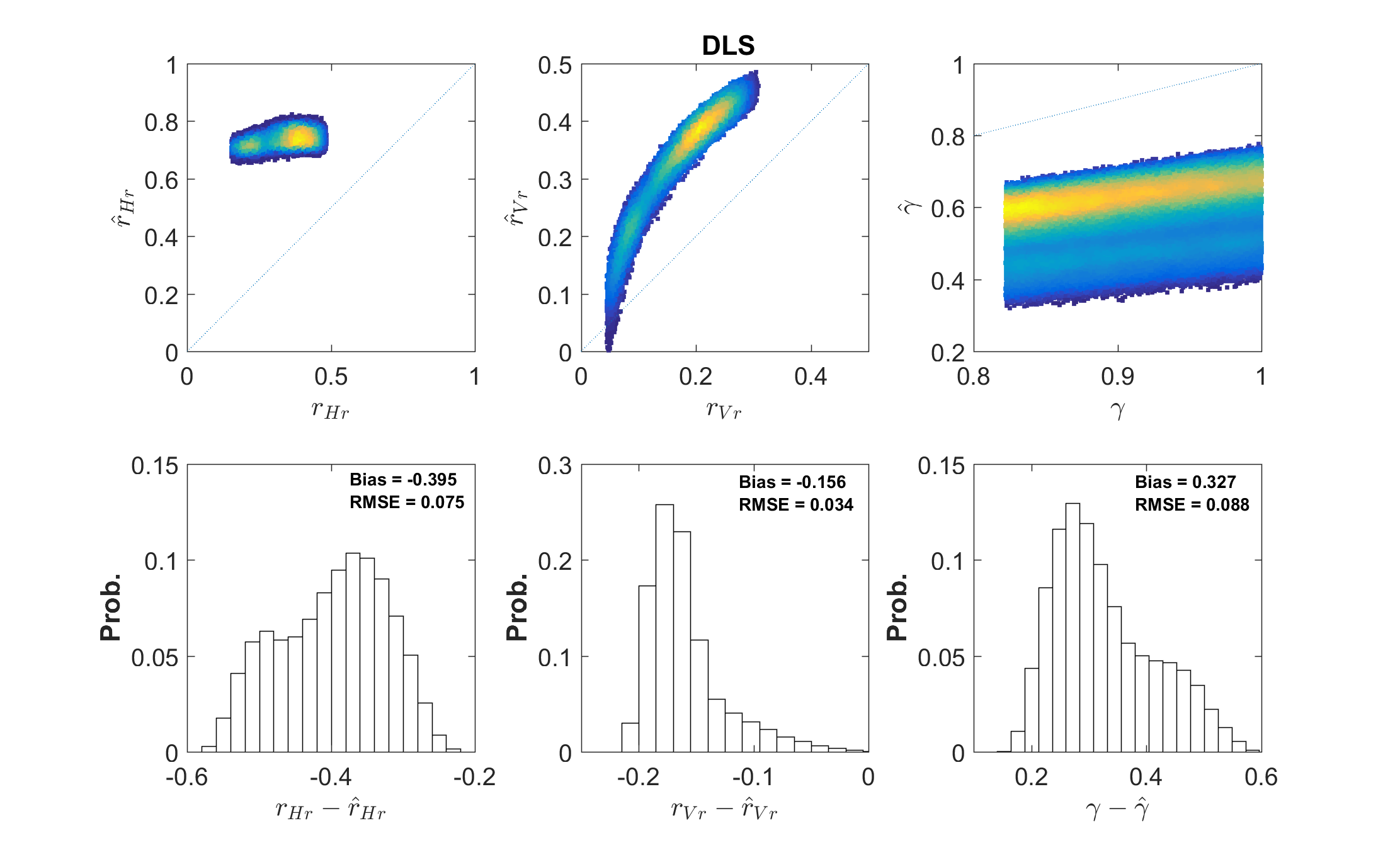
Figure 6: Results of CMCA (top two rows) versus unconstrained DLS (bottom two rows) retrievals of the rough soil reflectivity at horizontal ($r_{Hr}$) and vertical ($r_{Vr}$) polarization and the vegetation transmissivity $\gamma$, obtained via a controlled Monte Carlo experiment.

Figure 6 compares the results of CMCA with DLS solutions for $0<\text{VWC}<1.5$ kg m^-2 over all soil types for 5e+5 random inversion scenarios, where both channels are considered to be equally important. We first found that for the unconstrained DLS, involving both channels independently, may not necessarily decrease the retrieval error due to the ill-conditioning of the inversion, which often renders the information content of one channel ineffective. For example in Figure 6 (third row, first column), we can see that the retrieved $\hat{r}_{rH}$ through the DLS approach does not contain meaningful information. However, because of the used Tikhonov regularization in CMCA, the condition number of the problem is increased and the retrievals of the reflectivity values at both channels are correlated well with the reference.

The results in Figure 6 verify our earlier finding that the unconstrained underdetermined inversion of the $\tau$-$\omega$ model could lead to biased results. It is shown that for high values of vegetation transmissivity, the soil moisture and VWC are likely to be overestimated by DCA. We need to note that with a proper bias correction, the RMSE values are in an admissible range. For example, we can see that the bias and RMSE in DCA retrievals of $r_{Vr}$ are -0.16 and +0.034, respectively, which are around 50 and 11% of its feasible range of variability.

We extend the above analysis to different NRCS soil types (Figure 7). To that end, the biases and RMSE values are obtained for 5e+5 randomized retrievals for each soil type over three ranges of VWC. Overall, the results are almost unbiased and the RMSE is in a reasonable range. For almost all soil types, the bias (RMSE) remains below 5 and 1% (25 and 35%) in retrievals of the soil reflectivity and vegetation transmissivity, respectively.

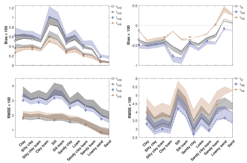
Figure 7: The normalized quality metrics by their feasible range for the CMCA retrievals over different soil types and VWC. The results are shown at horizontally ($H$) and vertically ($V)$ polarizations for the dual ($D$) and single ($S$) channel retrievals. The lines with markers show the results for VWC ranging from 1.5 to 3.0 kg m^-2, while the upper and lower bounds of the shaded areas show the results for higher (3.0–5.0 kg m^-2) and lower (0–1.5 kg m^-2) ranges of VWC.

In the first column of Figure 7, we can see that both bias and RMSE of the retrieved reflectivity values are improved as the soil clay content is decreased. This observation implies that the quality of the soil moisture retrievals highly depends on proper determination of the reflectivity bounds, which are tighter for sandy soils and wider for silty soils. We also observe that the retrievals normally tend to systematically overestimate the surface soil reflectivity, even though the biases are sufficiently small. The quality of both dual and single channel retrievals are also examined and it is found that the uncertainties are reduced when the vertical channel is involved, which can be due to its tighter bounds. We also found that the quality of the retrieved reflectivity values is not excessively sensitive to the VWC when it remains below 3 kg m^-2; however, the bias and RMSE decrease by 20% and 16%—when VWC increases from 3.0 to 5.0 kg m^-2, respectively.

In the second column of Figure 7, the quality metrics for retrievals of the vegetation transmissivity ($\gamma$) are shown, which do not exhibit any significant trend as a function of soil type. However, the metrics are slightly increased over silty soils–mainly because retrievals of $\gamma$ and soil reflectivity values are not independent. The retrievals are almost unbiased; however, tend to systemically underestimate $\gamma$, except for soils with high sand content. The retrievals in vertical polarization provide minimum biases but the horizontal channel leads to smaller RMSE values.

4.2 Windowed Retrievals

To examine the results of the algorithm for a windowed retrieval, we use surface soil moisture and temperature time series that are obtained from a gauge station (N 35^∘13^′, W92^∘55^′) of the Soil Climate Analysis Network (SCAN) in Arkansas, United States (Figure 8, first and second rows). We confine our consideration to 120 days of hourly surface soil moisture and temperature observations at depth 5 cm from 03/08/2017 to 07/06/2017. In this period, the volumetric soil moisture content changes from 0.194 to 0.435, which results in $0.60\leq r_{Hr}\leq 0.70$ and $0.44\leq r_{Vr}\leq 0.57$ using the dielectric model [43]. In the site, the first 20 cm of the soil is largely silty soil with clay content 4.1%.

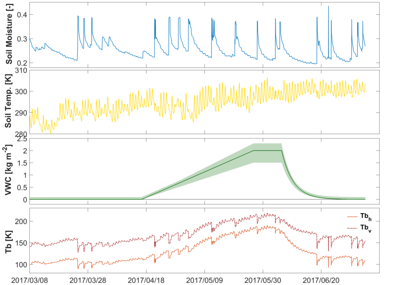
Figure 8: The hourly time series of surface soil moisture (first row), soil temperature (second row), vegetation water content (third row), and simulated brightness temperatures at 1.4 GHz for both horizontal (Tb_h) and vertical polarization (Tb_v) (fourth row). The data are from a SCAN gauge station in Arkansas, United States. The soil moisture and temperature are measured in depth 0.05 cm. The assumptions about the VWC and its uncertainties, shown in shaded area, are synthetic.

To construct an inversion scenario, we hypothetically assumed that the true VWC remains zero during the first 40 days and linearly increases to 2 kg m^-2 in the next 40 days. Then, the VWC remains constant for 10 days and decays exponentially in the last 30 days with a rate of 0.25 kg m^-2 d^-1. We consider 15% multiplicative uncertainty around the VWC (i.e., VWC_min=0.75 VWC, VWC_max=1.15 VWC) to define the box constraints for the vegetation transmissivity values. When the VWC is zero, we consider a non-symmetric bound from zero to 0.10 kg m^-2 (Figure 8, third row). Even though, the reconstructed problem might not be fully realistic as the signals of soil moisture and VWC are not actually coupled, the subsequent inversion experiment sheds light on how an a priori assumption about smoothness in temporal dynamics of the VWC can be used for improved soil moisture retrieval.

For windowed retrievals, the standard form of the CMCA in equation 10 can be expanded as follows:

$$\underset{\mathbf{r}_{pr},\,\mathbf{\gamma}}{\text{minimize}} \left\|\mathbf{e_{\tau}}-f(\mathbf{r}_{pr},\,\boldsymbol{\gamma})\right\|_{2}^{2}+\lambda_{1}\left\|\mathbf{r}_{pr}\right\|_{2}^{2}+\lambda_{2}\left\|\mathbf{D}\boldsymbol{\gamma}\right\|_{2}^{2}$$ (11)

subject to $$\boldsymbol{r}_{pl}\preceq\mathbf{r}_{pr}\preceq\boldsymbol{r}_{pu}\,\,,\,\,\boldsymbol{\gamma}_{l}\preceq\boldsymbol{\gamma}\preceq\boldsymbol{\gamma}_{u}.$$

where $\mathbf{e}_{\tau}=\left(e_{1},\,\ldots,e_{t}\right)^{T}\in\mathbb{R}^{t}$, $\mathbf{r}_{pr}=\left(r_{Hr1},\ldots,r_{Hrt},r_{Vr1},\ldots,r_{Vrt}\right)^{T}\in\mathbb{R}^{2t}$, $\boldsymbol{\gamma}=\left(\gamma_{1},\,\ldots,\gamma_{t}\right)^{T}\in\mathbb{R}^{t}$, and

$$\mathbf{D}=\begin{bmatrix}1&-2&1&\cdots&0\\ \vdots&\ddots&\ddots&\ddots&\vdots\\ 0&\cdots&1&-2&1\end{bmatrix}\in\mathbb{R}^{(t-2)\times t}.$$ (12)

Here, we chose a second order derivative operator for $\mathbf{D}$ to account for the smoothness in temporal variability of the VWC. This choice enables to project a large body of the time series of the VWC to zero and results in a smaller 2-norm than a first-order derivative. Choosing the first-order derivative often results in a piece-wise linear retrievals between the soil moisture jumps (not shown here). Note that the above formulation allows for the use of two different regularization parameters, which is necessary as the 2-norm of $\mathbf{r}_{rp}$ and $\mathbf{D}\gamma$ are significantly different and need to be scaled properly. Through a trial and error, we chose $\lambda_{1}$=1e-7 and $\lambda_{2}$=5e+2. To make the retrieval experiment computationally tractable, we solved problem 11 for non-overlapping windows of 10 days.

The results show minor bias of less than 6% in retrievals of reflectivity and transmissivity values (Figure 9). We observe that the peaks are captured well. However, when the soil moisture decaying limb is relatively long, the retrievals often overestimate the low values of soil moisture at the end of the limb, which is consistent with our previous finding about the effects of the preferential solution space in LS inversion of the $\tau$-$\omega$ model. As previously noted, we also observe that the retrievals of soil reflectivity values in vertical polarization are less biased.

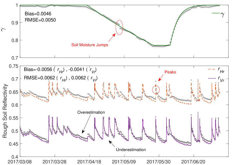
Figure 9: The CMCA windowed retrievals of the vegetation transmissivity ($\gamma$, top row) and the rough surface soil reflectivity values ($r_{Hr}$ and $r_{Vr}$, bottom row) for the shown boundary conditions in Figure 9. Retrievals of $\gamma$ are sensitive to the jumps in soil moisture content–especially when the VWC is relatively high. The results indicate that the peaks of the soil reflectivity values are well retrieved, while the the reflectivity values are slightly overestimated at the end of the soil moisture recession limbs.

The relative RMSE in retrievals of transmissivity and reflectivity values is around 3 and 6% of their variability range. Overall, the experiment reaffirms that the quality of the retrievals depends on accurate characterization of the bounds and magnitude of the VWC. For example, the RMSE for retrieval of $r_{Vr}$ reduces from 0.011 to 0.0034 (70%), when the mean of the VWC decreases from 2.5 to 0.1 kg m^-2. When the multiplicative uncertainty factor is increased from 5 to 30%, the RMSE of $r_{Vr}$ is also increased by $\sim 70$% from 0.0042 to 0.007. We need to note that, even though this relative increase seems to be large, it is only about 3% of the bound width of $r_{Vr}\in\left[0.44,\,0.57\right]$. The largest errors in retrieval of VWC often occur, when soil moisture suddenly jumps due to a precipitation event over vegetative surfaces (Figure 9, first row).

4.3 Implementation for the SMAP Retrievals

In this subsection, we elaborate on implementation of the proposed algorithm for retrieval of surface soil moisture and VWC using the SMAP observations. We confine our consideration to the SMAP observations over CONUS, where we can use multi-layer soil characteristics at a resolution of 1 km.

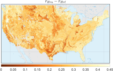
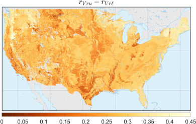
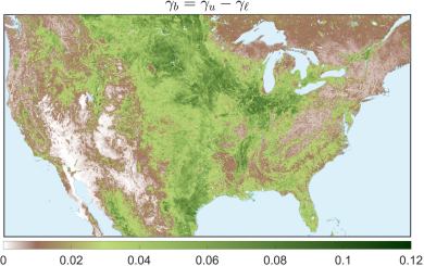
Figure 10: The static bounds of the rough surface soil reflectivity at $f=1.4$ GHz for horizontal ($r_{Hru}-r_{Hr\ell}$) and vertical ($r_{Vru}-r_{Vr\ell}$) polarization channels over the CONUS at 1-km grid, where we assumed that the soil moisture varies between the permanent wilting point and the soil porosity. The monthly climatology of the vegetation transmissivity bound ($\gamma_{b}=\gamma_{u}-\gamma_{\ell}$, second row) in month of June at resolution 0.05^∘.

We use the soil dataset by Miller and White [52] that contains compiled information from the State Soil Geographic (STATSGO) data by the Natural Resources Conservation Service (NRCS) of the United States Department of Agriculture. This dataset contains information about soil texture classes, clay fraction, and porosity at grid resolution 1 km for 11 layers from surface to the depth of 2 m. The first layer represents the top soil from 0 to 5 cm depth. To compute the reflectivity bounds, we consider that the soil moisture varies between the permanent wilting point and the soil porosity. Clearly, this bound could be tightened in the future, for example by assuming that the soil moisture varies between irreducible water content and natural saturation.

Figure 10 (first row) shows the static bounds of the vertically and horizontally polarized rough surface soil reflectivity values at frequency 1.4 GHz. Over the CONUS, the most abundant surface soil types are the loam (25.6%), silt loam (25.0%) and sandy loam (23.0%). The areal percentage of other surface soil types remain below 6%. The used soil data report almost zero percentage of silt and sandy clay soils. Figure 11 shows the box plot of the computed reflectivity bounds for the existing soil types. As is evident, the median and width of the reflectivity bounds reduce when the clay content increases. It appears that there is not any significant difference between the width of the bounds for the horizontal and vertical polarization. The widest bounds belong to the sandy loam, loamy sand, and loam—largely due to the dynamic range of their soil moisture and clay content. The distribution of the bounds is often asymmetric with negative skewness.

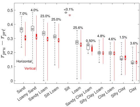
Figure 11: Reflectivity bounds for soil types over the CONUS at horizontal (black dashed lines, $r_{Hru}-r_{Hr\ell}$) and vertical (solid red lines, $r_{Vru}-r_{Vr\ell}$) polarization. The central point is the median, the boxes span between the first and third quartiles, and the whiskers are the min and max values. The numerics are the areal percentage of the surface soil types.

Unlike the static nature of the soil reflectivity bounds, the bounds on vegetation transmissivity can be defined dynamically. To that end, we use 16-day NDVI data at resolution 0.05^∘ from the Moderate Resolution Imaging Spectroradiometer (MODIS) sensor on board the Terra satellite [MOD13C1-V6, 53]. The pixel-level monthly maximum and minimum values are computed using all available data from 2002 to 2017. The monthly timescale is chosen to address slow changes in VWC while providing sufficiently tight bounds for the retrievals. We used the relationships by Jackson et al. [35] and Hunt et al. [39] to convert the NDVI to foliage and stem water content respectively. Then the VWC is transformed to the vegetation transmissivity by assuming $b=0.1$, where $\tau=b\text{\,VWC}$, $\gamma=\exp\left(-\tau\,\sec\phi\right)$ and $\phi=40^{\circ}$. The bound on climatology of the vegetation transmissivity ($\gamma_{max}-\gamma_{min}$) in the month of June is shown in Figure 10 (bottom row). It is clear that the cultivated croplands and natural grasslands show maximum amount of monthly variability during a growing month, while the bound width is minimal for example over the deciduous broadleaf forest of the Appalachian Mountains.

   

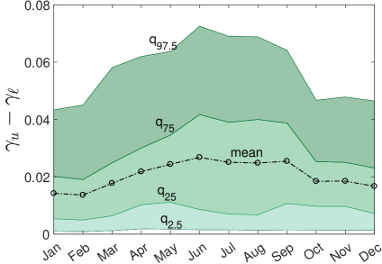
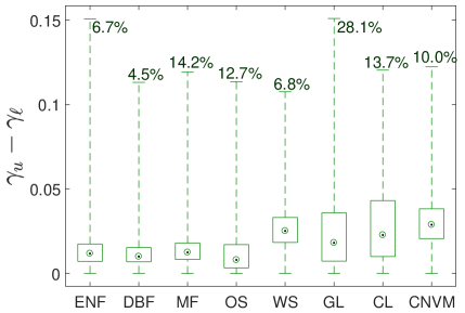
Figure 12: climatology of the vegetation transmissivity bounds ($\gamma_{b}=\gamma_{u}-\gamma_{\ell}$) for different months of the year (left) and dominant IGBP land cover types (right) over the CONUS. The land cover types include the evergreen needleleaf forest (ENF), deciduous broadleaf forest (DBF), mixed forest (MF), open shrublands (OS), woody savannas (WS), grasslands (GL), croplands (CL), and cropland/natural vegetation mosaic (CNVM), where the numerical values denote the areal percentage of each land cover type.

For improved understanding of the spatiotemporal dynamics of the bounds of the vegetation transmissivity, Figure 12 (left) shows monthly changes in the spatial mean of $\gamma_{b}=\gamma_{u}-\gamma_{l}$ over the CONUS. The bounds are relatively tight as the width is smaller than 0.10. We can see that the difference between percentile 97.5 and 2.5 increases from $\sim 0.04$ to 0.08 from dormant to growing months and reaches to its maximum around June and July.

We also study the distribution of $\gamma_{b}$ over dominant land cover types (Figure 12, right). To that end, the classification by the International Geosphere-Biosphere Programme (IGBP) is adopted. This classification over the CONUS is obtained from the MODIS combined product MCD12C1 provided by the NASA’s Land Processes Distributed Active Archive Center. The maximum values of $\gamma_{b}$ reaches to 0.15 over the evergreen needless forests and grasslands. The grasslands and croplands cover more than 40% of the CONUS and have the widest interquartile range of $\gamma_{b}$; even though, the extremum values are not significantly different than the other surface types.

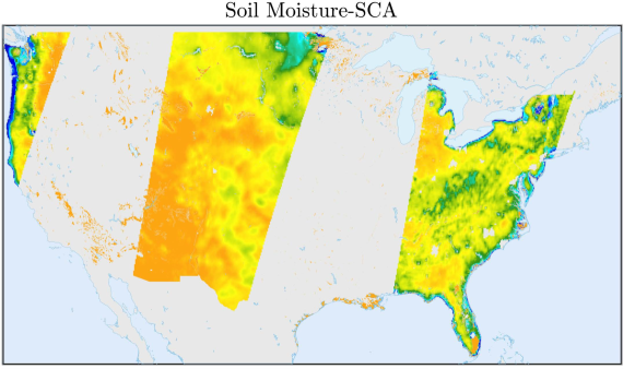
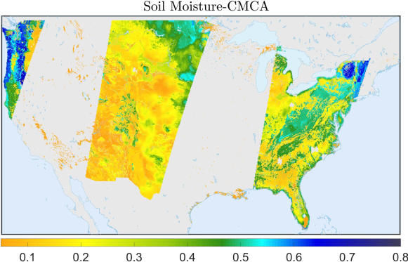
Figure 13: The enhanced SMAP (first row) and CMCA (second row) soil moisture retrievals on 06/01/2016, at nominal resolution 9 and 1 km, respectively.

We examined the initial results of the algorithm for a retrieval experiment using SMAP observations over the CONUS. We focused on the enhanced level-III SMAP radiometric data and soil moisture retrievals [54] with nominal grid resolution of 9 km on 06/01/2016 (Figure 13, first row), which are derived by interpolating the values from the nearest 6 instantaneous fields of view (IFOV) of the SMAP radiometer footprints. As previously explained, the VWC content in the SMAP data (Figure 15, first row) is a 10-day climatology from MODIS data that is averaged to match the soil moisture resolution at 9 km. One advantage of the CMCA approach is that the resolution of the retrievals is not only a function of the native resolution of radiometer but also the resolution of constraints. For the case of the SMAP retrieval over the CONUS, we have static constraints for the soil reflectivity values at resolution 1 km and dynamic constraints of vegetation transmissivity at resolution 1 to 5 km. Here, we map the SMAP radiometric observations and vegetation transmissivity bounds onto a 1 km grid using the nearest neighbor interpolation to conduct retrievals at this nominal resolution.

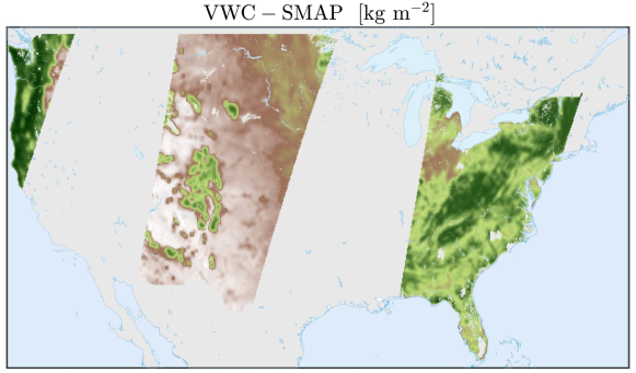
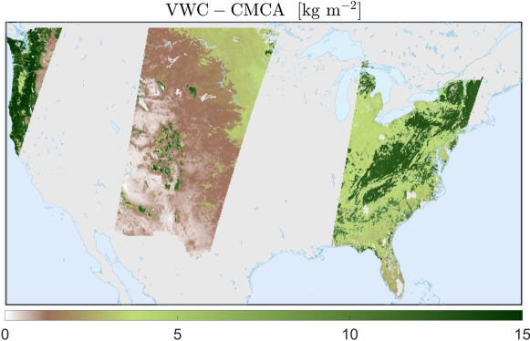
Figure 14: The ancillary VWC data (first row) at resolution of 9 km reported in enhanced SMAP products and the results of CMCA retrievals of the VWC (second row) at 1 km resolution on 06/01/2016.

The CMCA retrievals of soil moisture and VWC retrievals at 1 km grid resolution are shown in Figure 13 and 14 (second rows). The CMCA retrievals provide a high-resolution representation of both soil moisture and VWC, due to the high-resolution constraints. To quantify the retrieved extra high-resolution soil moisture details, Figure 15 shows the local variability of the retrievals at different scales, ranging from 2 to 64 km. The retrieved soil moisture fields are basically broken down into non-overlapping neighborhoods of size 2 to 64 km and then the expected values of the standard deviation are computed within those neighborhoods.

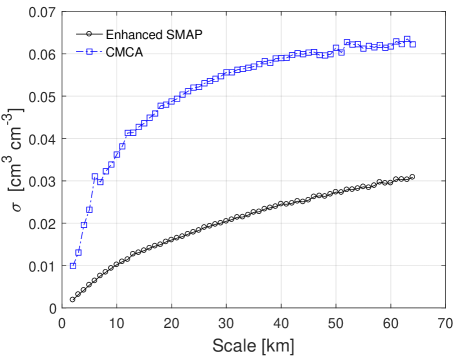
Figure 15: Standard deviations ($\sigma$) of the soil moisture local fluctuations in Figure 14 at different scales.

The computed standard deviations are measures of the variability of the soil moisture fluctuations around its local mean at different scales. As expected, the standard deviation increases as a function of scales and reaches to a plateau, when the analysis scale becomes greater than the largest dominant mode of the soil moisture spatial variability. In the presented retrieval experiment, the calculated standard deviations of the CMCA retrievals are 2 to 3 times larger than their counterparts for the enhanced product. The difference increases from 0.01 to 0.03 [cm³ cm^-3] as the analysis scale increases. This difference is an indication that some extra high-resolution details can be recovered by the CMCA. However, understanding the signal to noise ratio of this high-resolution details requires a thorough comparison of the retrievals against ground-based observations.

An important observation is that the CMCA slightly overestimates the SMAP product. This overestimation is pronounced over the evergreen needleleaf forests of the Pacific coast ranges, Colorado forests, and the deciduous broadleaf forests of the Appalachians, where the VWC is generally above 5 kg m^-2 and thus the $\tau$-$\omega$ model cannot fully explain the radiometric signature of the soil moisture. However, there are also overestimations in croplands of the Northern Minnesota and North Dakota, where the VWC is less than 5 kg m^-2.

4.4 SMAP Validation Experiments

To validate the retrieved soil moisture, we used the soil moisture gauge data from the International Soil Moisture Network (ISMN) database [55, 56]. Screening that data, we identified 206 gauges with good quality flags that provide soil moisture observations within the SMAP swath width on 06/01/2016 (Figure 16). These gauges are from U.S. Climate Reference Network (USCRN), Soil Climate Analysis Network (SCAN), Snow Telemetry (SNOWTEL), Interactive Roaring Fork Observation Network (iRON), and Cosmic-ray Soil Moisture Observing System (COSMOS). The gauge observations, reported at Coordinated Universal Time, are interpolated linearly onto the SMAP scanning times.

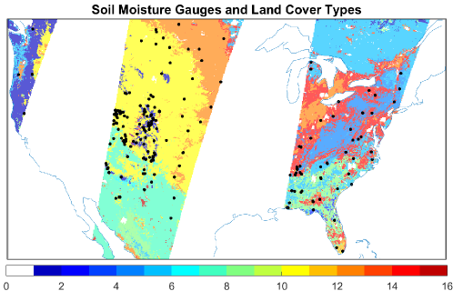
Figure 16: Location of the soil moisture gauge stations from the ISMN database and the IGPB land cover types, where labels 10, 12 and 14 denote grasslands, croplands, and cropland/natural vegetation mosaic, respectively.

Among these gauges, 110 gauges are over grasslands and croplands where the VWC is less than 5 kg m^-2. Comparing these gauge data with the nearest pixels of soil moisture retrievals in Figure 13 indicates that the bias in CMCA is around +0.02, while it is around -0.025 in the SMAP retrievals and the standard deviation of both retrievals is around 0.14 (Figure 16).

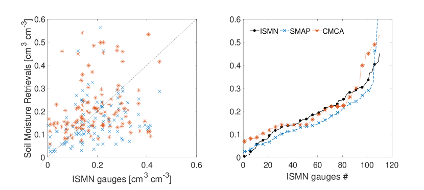
Figure 17: ISMN soil moisture gauge data versus CMCA and SMAP retrievals over grass and croplands (left) and sorted data (right) showing the pattern of over and underestimations.

The results show that CMCA overestimates (underestimate) the soil moisture when the gauge measurements are below 0.15 (above 0.3). The overestimation could be due to the fact that the lower bound of the soil moisture retrievals is set to the soil permanent wilting point, which is 0.05 and 0.30 [cm³ cm^-3] in sandy and clayey soils (Table 1). We also confined the upper bound of soil moisture retrievals to the soil porosity, which is generally higher than the soil natural saturation. Table 2 reports the sensitivity of the error statistics to the lower and upper bounds of soil moisture retrievals, which are shifted by two multiplicative parameters.

$c_{l}$-$c_{h}$	1-0.80	1-0.90	0-0.7	0-0.80	0-0.90	0.7-0.7	0.80-0.80	0.85-0.85	0.90-0.90
Bias	0.008	0.014	-0.029	-0.022	-0.015	-0.016	-0.004	0.002	0.007
RMSE	0.126	0.135	0.118	0.127	0.137	0.117	0.125	0.130	0.135

Table 2: Error statistics of the CMCA retrievals against the gauge data for different bounds, where the soil permanent wilting point and porosity are multiplied by $c_{l}$ and $c_{h}$ respectively.

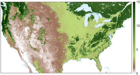
Figure 18: The derived VWC from 16-day MODIS NDVI data on 06/01/2016.

To validate the retrievals of the VWC we use as a reference the derived VWC from the 16-day NDVI data available on 05/24 and 06/09/2016 (Figure 18). To this end, we first obtained a temporal weighted average of the NDVI values and then derived the VWC at $0.05^{\circ}$-degree. We see that there are differences between the observations and the climatology of the VWC (Figure 14, first row). The climatology map underestimates the observed VWC, especially over grass and croplands, which leads to overestimation of the vegetation transmissivity and thus underestimation of soil moisture. This issue could be exacerbated due to coarse-graining of the NDVI data, knowing that the VWC is quadratically related to the NDVI [35]. Visual inspection shows that the retrieved vegetation transmissivity values by CMCA are consistent with the MODIS observations and capture well the VWC of croplands. The bias and RMSE values for the CMCA retrievals are 0.38 and 1.5 kg m^-2 over the pixels where the VWC is below 5 kg m^-2. These statistics for the climatology of VWC are -0.83 and 1.8 kg m^-2 for the bias and RMSE.

5 Discussion and Concluding Remarks

The existing single channel algorithms (SCA) for passive microwave soil moisture retrievals often rely on climatology of VWC as a priori knowledge, which is obtained through ancillary NDVI data. On the other hand, the double channel algorithms (DCA) retrieve both soil moisture and VWC simultaneously without using any a priori knowledge about the soil type and vegetation density, which could lead to biased results.

We presented a new constrained passive microwave soil moisture retrieval algorithm that closes the gaps between these two widely used algorithmic approaches. This algorithm conditions its retrievals to the static physical properties of surface soil and can account for uncertainties in climatology of the VWC. A smoothing norm regularization is proposed to extend the algorithm for soil moisture retrievals over a window of time to formally account for slow varying dynamics of VWC in grass and croplands. In this paper, we validated the outputs of the algorithm through a series of synthetic and an initial ground-validation experiments. Using the SMAP observations over the CONUS, we demonstrated that the algorithm can lead to super-resolved retrievals of soil moisture and VWC given high-resolution constraints.

Any operational application of CMCA requires a thorough calibration of the parameters based on validation against ground-based gauge observations. From an algorithmic stand point, the quality of the CMCA retrievals depends highly on the a priori bounds that characterize feasible range of the surface soil reflectivity and transmissivity of the overlying vegetation. Study of the climatology of the ground-based soil moisture data and use of much higher-resolution NDVI data (e.g., 250 m from the MODIS sensor) could lead to improved characterization of the constraints. Since we observed that the calculated bounds are not distributed uniformly, probabilistic consideration of the bounds could also lead to improved retrievals. Moreover, the accuracy of the inversion of the $\tau$-$\omega$ model is related multiplicatively to the accuracy of the surface soil temperature. Therefore, extension of the approach to a combined retrieval algorithm that optimally fuses multiple sources of reanalysis surface temperatures could be another line for future research.

References

References

- Gleick [1998] P. Gleick, Water in crisis: paths to sustainable water use, Ecol. Appl. 8 (1998) 571–579.
- Liu et al. [2015] Y. Liu, Z. Pan, Q. Zhuang, D. G. Miralles, A. J. Teuling, T. Zhang, P. An, Z. Dong, J. Zhang, D. He, L. Wang, X. Pan, W. Bai, D. Niyogi, Agriculture intensifies soil moisture decline in Northern China, Sci. Rep. 5 (2015) 11261.
- Trenberth [2011] K. Trenberth, Changes in precipitation with climate change, Clim. Res. 47 (2011) 123–138.
- Lin et al. [2016] L.-F. Lin, A. M. Ebtehaj, J. Wang, R. L. Bras, Soil Moisture Background Error Covariance and Data Assimilation in a Coupled Land-Atmosphere Model, Water Resour. Res Under revi (2016) 1309–1335.
- Lin et al. [2017] L.-F. Lin, A. M. Ebtehaj, A. N. Flores, S. Bastola, R. L. Bras, Combined Assimilation of Satellite Precipitation and Soil Moisture: A Case Study Using TRMM and SMOS Data, Mon. Weather Rev. 145 (2017) 4997–5014.
- Velpuri et al. [2016] N. M. Velpuri, G. B. Senay, J. T. Morisette, Evaluating New SMAP Soil Moisture for Drought Monitoring in the Rangelands of the US High Plains, Rangelands 38 (2016) 183–190.
- Nicolai-Shaw et al. [2017] N. Nicolai-Shaw, J. Zscheischler, M. Hirschi, L. Gudmundsson, S. I. Seneviratne, A drought event composite analysis using satellite remote-sensing based soil moisture, Remote Sens. Environ. 203 (2017) 216–225.
- Katul et al. [2012] G. G. Katul, R. Oren, S. Manzoni, C. Higgins, M. B. Parlange, Evapotranspiration: A process driving mass transport and energy exchange in the soil-plant-atmosphere-climate system, Rev. Geophys. 50 (2012).
- Schlesinger and Jasechko [2014] W. H. Schlesinger, S. Jasechko, Transpiration in the global water cycle, Agric. For. Meteorol. 189-190 (2014) 115–117.
- Falloon et al. [2011] P. Falloon, C. D. Jones, M. Ades, K. Paul, Direct soil moisture controls of future global soil carbon changes: An important source of uncertainty, Global Biogeochem. Cycles 25 (2011) n/a–n/a.
- Pastor and Post [1986] J. Pastor, W. M. Post, Influence of climate, soil moisture, and succession on forest carbon and nitrogen cycles, Biogeochemistry 2 (1986) 3–27.
- Njoku and Entekhabi [1996] E. G. Njoku, D. Entekhabi, Passive microwave remote sensing of soil moisture 184 (1996) 101–129.
- Le Vine et al. [2007] D. Le Vine, G. Lagerloef, F. Colomb, S. Yueh, F. Pellerano, Aquarius: An Instrument to Monitor Sea Surface Salinity From Space, IEEE Trans. Geosci. Remote Sens. 45 (2007) 2040–2050.
- Kerr et al. [2012] Y. H. Kerr, P. Waldteufel, P. Richaume, J. P. Wigneron, P. Ferrazzoli, A. Mahmoodi, A. A. Bitar, F. Cabot, C. Gruhier, S. E. Juglea, D. Leroux, A. Mialon, S. Delwart, A. Al Bitar, F. Cabot, C. Gruhier, S. E. Juglea, D. Leroux, A. Mialon, S. Delwart, The SMOS Soil Moisture Retrieval Algorithm, IEEE Trans. Geosci. Remote Sens. 50 (2012) 1384–1403.
- Entekhabi et al. [2010] D. Entekhabi, E. G. Njoku, P. E. O’Neill, K. H. Kellogg, W. T. Crow, W. N. Edelstein, J. K. Entin, S. D. Goodman, T. J. Jackson, J. Johnson, J. Kimball, J. R. Piepmeier, R. D. Koster, N. Martin, K. C. McDonald, M. Moghaddam, S. Moran, R. Reichle, J. C. Shi, M. W. Spencer, S. W. Thurman, L. Tsang, J. Van Zyl, The soil moisture active passive (SMAP) mission, Proc. IEEE 98 (2010) 704–716.
- Njoku and Kong [1977] E. G. Njoku, J.-A. Kong, Theory for passive microwave remote sensing of near-surface soil moisture, J. Geophys. Res. 82 (1977) 3108.
- Mo et al. [1982] T. Mo, B. J. Choudhury, T. J. Schmugge, J. R. Wang, T. J. Jackson, A model for microwave emission from vegetation-covered fields, J. Geophys. Res. 87 (1982) 11229–11237.
- Ulaby et al. [1982] F. T. Ulaby, R. K. Moore, A. K. Fung, Microwave Remote Sensing: Active and Passive Volume II: Radar Remote Sensing and Surface Scattering and Emission Theory, volume 2, 1982.
- Jackson and Schmugge [1991] T. J. Jackson, T. J. Schmugge, Vegetation effects on the microwave emission of soils, Remote Sens. Environ. 36 (1991) 203–212.
- Entekhabi and Njoku [1994] D. Entekhabi, E. G. Njoku, Solving the Inverse Problem for Soil Moisture and Temperature Profiles by Sequential Assimilation of Multifrequency Remotely Sensed Observations, IEEE Trans. Geosci. Remote Sens. 32 (1994) 438–448.
- Njoku and Li [1999] E. G. Njoku, L. Li, Retrieval of land surface parameters using passive microwave measurements at 6-18 GHz, Ieee Trans. Geosci. Remote Sens. 37 (1999) 79–93.
- Jackson et al. [2004] T. J. Jackson, D. Chen, M. Cosh, F. Li, M. Anderson, C. Walthall, P. Doriaswamy, E. R. Hunt, Vegetation water content mapping using Landsat data derived normalized difference water index for corn and soybeans 92 (2004) 475–482.
- van de Griend and Owe [1993] A. van de Griend, M. Owe, Determination of microwave vegetation optical depth and single scattering albedo from large scale soil moisture and Nimbus/SMMR satellite observations, Int. J. Remote Sens. 14 (1993) 1875–1886.
- Karam et al. [1992] M. A. Karam, A. K. Fung, R. H. Lang, N. S. Chauhan, Microwave Scattering Model for Layered Vegetation, IEEE Trans. Geosci. Remote Sens. 30 (1992) 767–784.
- van de Griend et al. [1996] A. van de Griend, M. Owe, J. de Ruiter, B. Gouweleeuw, Measurement and behavior of dual-polarization vegetation optical depth and single scattering albedo at 1.4- and 5-GHz microwave frequencies, IEEE Trans. Geosci. Remote Sens. 34 (1996) 957–965.
- Jackson [1993] T. J. Jackson, III. Measuring surface soil moisture using passive microwave remote sensing, Hydrol. Process. 7 (1993) 139–152.
- Levenberg [1944] K. Levenberg, A method for the solution of certain non-linear problems in least squares, Q. Appl. Math. 2 (1944) 164–168.
- Marquardt [1963] D. W. Marquardt, An Algorithm for Least-Squares Estimation of Nonlinear Parameters, J. Soc. Ind. Appl. Math. 11 (1963) 431–441.
- Tikhonov and Arsenin [1978] A. N. Tikhonov, V. Y. Arsenin, Solutions of Ill-Posed Problems, Math. Comput. 32 (1978) 1320–1322.
- Piles et al. [2010] M. Piles, M. Vall-llossera, A. Camps, M. Talone, A. Monerris, Analysis of a Least-Squares Soil Moisture Retrieval Algorithm from L-band Passive Observations, Remote Sens. 2 (2010) 352–374.
- Konings et al. [2016] A. G. Konings, M. Piles, K. Rötzer, K. A. McColl, S. K. Chan, D. Entekhabi, Vegetation optical depth and scattering albedo retrieval using time series of dual-polarized L-band radiometer observations, Remote Sens. Environ. 172 (2016) 178–189.
- Enr [2014] SMAP Handbook: Mapping Soil Moisture and Freezs/Thaw from Space, National Aeronautics and Space Administration, Jet Propulsion Laboratory, California Institute of Technology, 2014.
- Wigneron et al. [2017] J.-P. Wigneron, T. Jackson, P. O’Neill, G. D. Lannoy, P. de Rosnay, J. Walker, P. Ferrazzoli, V. Mironov, S. Bircher, J. Grant, M. Kurum, M. Schwank, J. Munoz-Sabater, N. Das, A. Royer, A. Al-Yaari, A. A. Bitar, R. Fernandez-Moran, H. Lawrence, A. Mialon, M. Parrens, P. Richaume, S. Delwart, Y. Kerr, Modelling the passive microwave signature from land surfaces: A review of recent results and application to the l-band smos & smap soil moisture retrieval algorithms, Remote Sensing of Environment 192 (2017) 238 – 262.
- Kerr and Njoku [1990] Y. Kerr, E. Njoku, A semiempirical model for interpreting microwave emission from semiarid land surfaces as seen from space, IEEE Trans. Geosci. Remote Sens. 28 (1990) 384–393.
- Jackson et al. [1999] T. J. Jackson, D. M. L. Vine, A. Y. Hsu, A. Oldak, P. J. Starks, C. T. Swift, J. D. Isham, M. Haken, Soil moisture mapping at regional scales using microwave radiometry: the southern great plains hydrology experiment, IEEE Transactions on Geoscience and Remote Sensing 37 (1999) 2136–2151.
- Van de Griend and Wigneron [2004] A. Van de Griend, J.-P. Wigneron, The b-factor as a function of frequency and canopy type at H-polarization, IEEE Trans. Geosci. Remote Sens. 42 (2004) 786–794.
- Crow et al. [2005] W. T. Crow, S. Chant, D. Entekhabi, A. Hsu, T. J. Jackson, E. Njoku, P. O’Neill, J. Shi, An observing system simulation experiment for hydros radiometer-only soil moisture and freeze-thaw products 4 (2005) 2737–2740.
- Jackson et al. [2010] T. J. Jackson, M. H. Cosh, R. Bindlish, P. J. Starks, D. D. Bosch, M. Seyfried, D. C. Goodrich, M. S. Moran, J. Du, Validation of Advanced Microwave Scanning Radiometer Soil Moisture Products, IEEE Trans. Geosci. Remote Sens. 48 (2010) 4256–4272.
- Hunt et al. [1996] E. R. Hunt, S. C. Piper, R. Nemani, C. D. Keeling, R. D. Otto, S. W. Running, Global net carbon exchange and intra-annual atmospheric CO 2 concentrations predicted by an ecosystem process model and three-dimensional atmospheric transport model, Global Biogeochem. Cycles 10 (1996) 431–456.
- Calvo-Alvarado et al. [2008] J. C. Calvo-Alvarado, N. G. McDowell, R. H. Waring, Allometric relationships predicting foliar biomass and leaf area:sapwood area ratio from tree height in five Costa Rican rain forest species, Tree Physiol. 28 (2008) 1601–1608.
- Choudhury et al. [1979] B. J. Choudhury, T. J. Schmugge, A. Chang, R. W. Newton, Effect of surface roughness on the microwave emission from soils, J. Geophys. Res. 84 (1979) 5699.
- Dobson et al. [1985] M. C. Dobson, F. T. Ulaby, M. T. Hallikainen, M. A. El-Rayes, Microwave Dielectric Behavior of Wet Soil-Part II: Dielectric Mixing Models, IEEE Trans. Geosci. Remote Sens. GE-23 (1985) 35–46.
- Mironov et al. [2009] V. L. Mironov, L. G. L. Kosolapova, S. S. V. Fomin, Physically and Mineralogically Based Spectroscopic Dielectric Model for Moist Soils, IEEE Trans. Geosci. Remote Sens. 47 (2009) 2059–2070.
- Mironov et al. [2013] V. L. Mironov, P. P. Bobrov, S. V. Fomin, A. Y. Karavaiskii, Generalized refractive mixing dielectric model of moist soils considering ionic relaxation of soil water, Russ. Phys. J. 56 (2013) 319–324.
- Boyd and Vandenberghe [2004] S. Boyd, L. Vandenberghe, Convex Optimization, volume 25, 2004.
- Wigneron et al. [2000] J. P. Wigneron, P. Waldteufel, A. Chanzy, J. C. Calvet, Y. Kerr, Two-dimensional microwave interferometer retrieval capabilities over land surfaces (SMOS Mission), Remote Sens. Environ. (2000).
- Goldfeld et al. [1966] S. M. Goldfeld, R. E. Quandt, H. F. Trotter, Maximization by Quadratic Hill-Climbing, Econometrica 34 (1966) 541.
- Sorensen [1982] D. C. Sorensen, Newton’s Method with a Model of Trust Region modification, SIAM J. Numer. ANAL 19 (1982).
- Coleman and Li [1996] T. F. Coleman, Y. Li, An Interior Trust Region Approach for Nonlinear Minimization Subject to Bounds, SIAM J. Optim. 6 (1996) 418–445.
- Hansen [2010] P. C. Hansen, Discrete Inverse Problems: Insight and Algorithms, 2010.
- Saxton and Rawls [2006] K. E. Saxton, W. J. Rawls, Soil Water Characteristic Estimates by Texture and Organic Matter for Hydrologic Solutions, Soil Sci. Soc. Am. J. 70 (2006) 1569.
- Miller and White [1998] D. A. Miller, R. A. White, A Conterminous United States Multilayer Soil Characteristics Dataset for Regional Climate and Hydrology Modeling, Earth Interact. 2 (1998) 1–26.
- Didan [2015] K. Didan, MOD13C1 MODIS/Terra Vegetation Indices 16-Day L3 Global 0.05Deg CMG V006, 2015.
- O’Neill et al. [2018] P. E. O’Neill, S. K. Chan, E. G. Njoku, T. J. Jackson, B. R., SMAP Enhanced L3 Radiometer Global Daily 9 km EASE-Grid Soil Moisture, Version 2, 2018.
- Dorigo et al. [2011] W. A. Dorigo, W. Wagner, R. Hohensinn, S. Hahn, C. Paulik, A. Xaver, A. Gruber, M. Drusch, S. Mecklenburg, P. Van Oevelen, A. Robock, T. Jackson, The International Soil Moisture Network: A data hosting facility for global in situ soil moisture measurements, Hydrol. Earth Syst. Sci. (2011).
- Dorigo et al. [2013] W. Dorigo, A. Xaver, M. Vreugdenhil, A. Gruber, A. Hegyiová, A. Sanchis-Dufau, D. Zamojski, C. Cordes, W. Wagner, M. Drusch, Global Automated Quality Control of In Situ Soil Moisture Data from the International Soil Moisture Network, Vadose Zo. J. (2013).