The boundary conditions of viscous electron flow

Abstract

The sensitivity of charge, heat, or momentum transport to the sample geometry is a hallmark of viscous electron flow. Therefore hydrodynamic electronics requires a detailed understanding of electron flow in finite geometries. The solution of the corresponding generalized Navier-Stokes equations depends sensitively on the nature of boundary conditions. The latter can be characterized by a slip length $\zeta$ with extreme cases being no-slip $\left(\zeta\rightarrow 0\right)$ and no-stress $\left(\zeta\rightarrow\infty\right)$ conditions. We develop a kinetic theory that determines the temperature dependent slip length at a rough interface for Dirac liquids, e.g. graphene, and for Fermi liquids. For strongly disordered edges that scatter electrons in a fully-diffuse way, we find that the slip length is of the order of the momentum conserving mean free path $l_{ee}$ that determines the electron viscosity. For boundaries with nearly specular scattering $\zeta$ is parametrically large compared to $l_{ee}$. Since for all quantum fluids $l_{ee}$ diverges as $T\rightarrow 0$, the ultimate low-temperature flow is always in the no-stress regime. Only at intermediate $T$ and for sufficiently large sample sizes can the slip lengths be short enough such that no-slip conditions are appropriate. We discuss numerical examples for several experimentally investigated systems. To identify hydrodynamic flow governed by no-stress boundary conditions, we propse the transport through an infinitely long strip containing an impenetrable circular obstacle.

I Introduction

The fluid flow of liquids is governed by the laws of hydrodynamics. If collisions are sufficiently strong and lead to local thermalization, yet respect the laws of charge, energy, and momentum conservation, hydrodynamics should apply Forster . Inhomogeneous flow velocity profiles of the Couette and Poiseuille type, vorticity of flow, or turbulent flow are among the indicators of hydrodynamic behavior. Starting with the pioneering work by Gurzhi Gurzhi1968 in 1968, the theoretical foundations of electron hydrodynamics have been discussed for a range electronic systems deJong1995 ; Kashuba2008 ; Fritz2008 ; Mueller2009 ; Andreev2011 ; Davison2014 ; Torre2015 ; Kashuba2018 ; Briskot2015 ; Alekseev2016 ; Levitov2016 ; Scaffidi2017 ; Lucas2018 ; Narozhny2017 ; Lucas2016_1 ; Lucas2016_2 ; Derek2018 . For electron hydrodynamics to apply, electron-electron collissions should dominate. Thus, the temperature should be below $T_{{\rm ph}}$ where electron-phonon scattering starts violating energy and momentum conservation of the electronic subsystems. At the same time $T$ should be above $T_{{\rm imp}}$ where impurities dominate, violating momentum conservation. Only if $T_{{\rm imp}}<T_{{\rm ph}}$ is there a window for hydrodynamic electronics, explaining the need for ultra-clean materials.

Examples for recent experimental investigations of hydrodynamic electronics include the observation of non-local momentum relaxation in the delafossite PdCoO₂ Moll2016 and the Weyl semimetal WP₂ Gooth2017 , systems that are special because of their exceptionally low residual resistivity. In parallel, advances in the fabrication of high-quality graphene led to the observation of hydrodynamic Coulomb drag Titov2013 , violations of the Wiedeman Franz law for the thermal transport Crossno2016 and the Mott relation for the thermoelectric transport Ghahari2016 , a negative local resistance due to flow with vorticity Bandurin , and superballistic flow KrishnaKumar2017 . In graphene at the charge neutrality point and other Dirac systems, electron-hole puddles form due to disorder effects Martin2008 . These puddles result in a local variation of the chemical potential $\delta\mu$. To observe hydrodynamic effects, $\left|\delta\mu\right|<k_{B}T$ must hold - a condition achieved in current experiments Crossno2016 . A key common feature of all those experiments is the fact that finite geometries strongly affect the electron flow. In fact the sensitivity of the flow profile to boundaries has been a key strategy to identify hydrodynamic flow.

The theoretical modelling of viscous electron flow is often based on the solution of kinetic equations Mueller2009 ; Titov2013 ; Briskot2015 ; Alekseev2016 ; Levitov2016 ; Scaffidi2017 ; Link2018 . A very efficient description, particularly appropriate for complex geometries is based on the Navier-Stokes equations for the flow velocity $\mathbf{u}\left(\mathbf{r},t\right)$. For Lorentz and Galilei-invariant systems the Navier-Stokes equations are dictated by symmetry Forster . In the general setting, they can be derived from the kinetic equation, see e.g. Ref. Mueller2009 ; Briskot2015 . Not surprisingly, the solutions of these equations depend sensitively on the imposed conditions at the sample boundaries. Let $S$ be the boundary of the sample. Popular boundary conditions are the no-slip condition

$$\left.u_{\alpha}^{t}\right|_{S}=0,$$ (1)

where $\mathbf{u}^{t}=\mathbf{u}-\left(\mathbf{u}\cdot\mathbf{n}\right)\mathbf{n}$ is the tangential velocity of a boundary with normal vector $\mathbf{n}$, and the no-stress condition

$$\left.n_{\beta}\frac{\partial u_{\alpha}^{t}}{\partial x_{\beta}}\right|_{S}=0.$$ (2)

The no-slip condition is the relevant one for most liquid-solid interfaces. Liquid particles at the surface do not move with the fluid flow, an effect either explained in terms of surface roughness or due to attractive interactions between solid and liquid particles, see Ref. Zhu2002 ; Lauga2007 . On the other hand, the liquid flow near a liquid-gas interface is often characterized by the no-stress condition, i.e. the tangential stress at the interface is continuous. As discussed by Maxwell Maxwell1867 , a boundary condition, that includes both cases as limits is

$$\left.u_{\alpha}^{t}\right|_{S}=\zeta\left.n_{\beta}\frac{\partial u_{\alpha}^{t}}{\partial x_{\beta}}\right|_{S},$$ (3)

where $\zeta$ is the slip length.

Figure 1: Velocity profile $\bm{u}\left(y\right)$ of an electron liquid near the edge of a sample. The boundary condition for $\bm{u}\left(y\right)$ is given by Eq. (3) so that $u\left(y=0\right)=\zeta\frac{\partial u}{\partial y}$. The slip length $\zeta$ characterizes the behavior of a liquid near the edge. It corresponds to the length where the extrapolated velocity vanishes. Also depicted is the Knudsen layer - an approximately one mean free path thin layer along the boundary, where the collisions of particles with the wall are as important as collisions among each other (see also Fig. 6).

It corresponds to the length where the extrapolated boundary velocity vanishes (see Fig. 1). Clearly, $\zeta\rightarrow 0$ and $\zeta\rightarrow\infty$ correspond to no-slip and no-stress conditions, respectively. Since the origin of tangential stress in a fluid is purely visous, one expects that the slip length is another quantity that can be determined from kinetic theory, like diffusivities or viscosities. Indeed, for rarified gases, Maxwell found that $\zeta$ is essentially given by the momentum-conserving mean free path, a result fully consistent with numerical simulations Morris1992 . Other systems where a finite slip length is of relevance are classical fluids affected by soft hydrodynamic modes Nieuwoudt1984 ; Wolynes1976 polymer melts deGennes1979 , phononic liquids Levinson1977 and ${}^{3}{\rm He}$ at low temperatures in the normal and superfluid state HJensen1980 ; Einzel1984 ; Einzel1990 ; Einzel1997 . Ref. Delacretaz2017 reports that in the quantum Hall regime no-stress conditions must be applied to agree with known results for the quantized Hall conductance.

Let us demonstrate the importance of a finite slip length for the fluid flow for a simple example. Consider the flow of a two-dimensional system that is governed by the linear, stationary limit of the Navier Stokes equation. For a strip of width $w$, oriented along the $x$-direction, we have $\partial p/\partial x=-\eta\partial^{2}u_{x}/\partial y^{2}$. LL_Fluid Solving for $u_{x}$ with the boundary condition (3) we obtain

$$u_{x}=\frac{1}{8\eta}\left(w^{2}+4\zeta w-4y^{2}\right)\frac{\partial p}{\partial x},$$ (4)

if $\partial p/\partial x$ is constant. The total heat current $I$ is proportional to the integral

$$I\propto\int_{-w/2}^{w/2}dy\,u_{x}=\frac{1}{2\eta}\left(\frac{w^{3}}{6}+\zeta w^{2}\right)\frac{\partial p}{\partial x}.$$ (5)

The second contribution stems from a finite slip velocity at the boundaries. Only if $\zeta\ll w$, does the typical Poiseuille scaling $I\propto w^{3}$ (or $w^{d+1}$ for arbitrary dimensions) hold. Clearly, any hydrodynamic effect, such as e.g. the Gurzhi effect (as the $I\propto w^{d+1}$ scaling is called in the context of electron flow), that depends on stress created by momentum dissipation at the boundaries, is critically influenced by $\zeta$. To illustrate the importance of boundary conditions, expressed in terms of the slip length, we show in Fig. 2 the flow profiles of a wire of thickness $w$ through which passes a current $I$ for different slip lengths.

Figure 2: Flow profiles of a wire of thickness $w$ through which passes a current $I$. For no-slip boundary conditions a parabolic flow profile, typical for Poiseuille flow, is realized. With growing slip length the flow profile becomes flat, i.e. more similar to Ohmic flow.

In the context of electron hydrodynamics, the nature of the boundary conditions is unclear. On the one hand, Poiseuille type flow, observed in Refs. Moll2016 ; Gooth2017 supports at the least a very small slip length if compared to the characteristic size of the system. On the other hand, the absence of such flow in graphene was taken as evidence for a no-stress boundary with a very large slip length Bandurin .

In this paper we develop a kinetic theory to determine the slip length $\zeta$ for Dirac and Fermi liquids in two limits. In the first limit only a small fraction of tangetial momentum is transferred to the wall in electron-wall collisions, which are assumed to be elastic. This limit we call the nearly specular limit. In the opposite, the diffuse, limit all tangential momentum is lost. The two limits correspond to samples with almost smooth and strongly disordered edges. We find that the slip lengths grow with decreasing temperatures. For graphene at charge neutrality, in the nearly specular limit $\zeta\sim\ln^{6}\left(T_{\Lambda}/T\right)/T^{4}$, whereas in the diffuse limit $\zeta\sim l_{ee}\sim\ln^{3}\left(T_{\Lambda}/T\right)/T$. The logarithmic factor stems from a renormalization of the group velocity of electrons caused by interaction effects Sheehy2007 . $T_{\Lambda}=\Lambda/k_{B}$, where $\Lambda$ is an energy cut-off. For realistic parameters of graphene, the slip lengths are larger than $1\,\upmu\textrm{m}$ below $100\textrm{\,K}$, which leads us to the conclusion that for most geometries used so far it is more appropriate to assume no-stress than no-slip conditions at the boundaries. In addition we discuss the slip length of three and two dimensional Fermi liquids, the latter describing graphene at a finite chemical potential $\mu\gg k_{B}T$ and potentially the delafossite PdCoO₂ of Ref. Moll2016 . We find that in three dimensions the slip length grows as $T^{-2}$ in both the diffuse scattering and the nearly specular scattering limits, yet with a coefficient that depends on the nature of the boundary scattering. For a two dimensional Fermi liquid the slip length behaves as $T^{-2}/\ln\left(\epsilon_{F}/k_{B}T\right)$, due to the well known logarithmic suppression of the quasiparticle liftime Hodges1971 . Comparing Dirac and Fermi liquid, we find that in the diffuse scattering limit, the slip lengths of graphene away from charge neutrality are larger then those of charge neutral graphene below $100\textrm{\,K}$. In the nearly specular limit, the slip length of charge neutral graphene is larger than that of graphene away from charge neutrality at very low temperatures, however, here $\zeta$ is very large for both systems. If the momentum dissipation is due to edge roughness, we find that graphene at a finite chemical potential $\mu$ is more susceptible to the magnitude of the roughness, because here the electron wavelengths - governed by the energy scale $\mu$ - are smaller than the thermal electron wavelengths of charge neutral graphene. Summing up, we find that the slip length for electronic flow can always be written in the form

$$\zeta=f\left(\kappa\right)l_{ee}$$ (6)

with dimensionless ratio $\kappa=h^{2}h^{\prime d-1}/\lambda^{d+1}$ . $\kappa$ depends on the two length scales $h$ and $h^{\prime}$ that characterize the interface scattering (see Eq. (21) and Fig. 4) and the electron wavelength $\lambda$, respectively. The latter is strongly temperature dependent for graphene at the neutrality point ($\lambda=\hbar v/(k_{{\rm B}}T)$), while it corresponds to the Fermi wave length in the case of Fermi liquids ($\lambda=1/k_{{\rm F}}$). Here $v$ is the renormalized group velocity of the electrons (see Eq. (11) and the discussion below Eq. (12)). For the dimensionless function $f\left(\kappa\right)$ we find $f\left(\kappa\ll 1\right)=f_{0}/\kappa$, while $f\left(\kappa\rightarrow\infty\right)\rightarrow f_{\infty}$. We determine $f_{\infty}$ using the assumption of diffuse scattering. The numerical values for the coefficients $f_{0}$ and $f_{\infty}$ depend sensitively on the electronic dispersion relation and dimensionality of the system, but the overall behavior is found to be generic. We find for Dirac systems at the neutrality point $f_{0}\approx 0.008$ and $f_{\infty}\approx 0.6$. For two-dimensional Fermi liquids holds $f_{0}\approx 1.1$ and $f_{\infty}\approx 1.2$, while we obtain for three-dimensional Fermi liquids $f_{0}\approx 3$ and $f_{\infty}\approx 0.5$. For a boundary with intermediate scattering strength we expect $f\left(\kappa\right)$ to smoothly interpolate between the two limits, with a crossover for $\kappa\sim{\cal O}\left(1\right)$.

Thermal currents in charge neutral graphene

In a Galilei-invariant system, the drift velocity $\bm{u}$ is proportional to the electric current:

$$\bm{j}=ne\bm{u},$$ (7)

where $n$ is the particle density. This means that the hydrodynamic flow of a Fermi liquid can be probed by measuring the electric current $\bm{j}$. A key aspect of electron hydrodynamics in graphene at charge neutrality is that here the heat current takes the place of mass or charge current in conventional systems. The heat current is proportional to the momentum density and therefore conserved in electron-electron interactions. As a result the thermal conductivity at the neutrality point is infinite, if the momentum is not dissipated by other mechanisms such as impurities or boundary scattering M=0000FCller2008 . This is a direct consequence of the linear dispersion of graphene. The drift velocity $\bm{u}$ is connected to the heat current Briskot2015 via

$$\bm{j}_{E}=\frac{3n_{E}\bm{u}}{2+u^{2}/v^{2}}.$$ (8)

Furthermore, at charge neutrality, no hydrodynamic flow $\bm{u}$ can be excited by applying an electric field because the same number of hole-like excitations flows in one direction as electrons in the other. A temperature difference, however, can be thermodynamically related to a pressure difference. This qualitatively different behavior of the thermal and electric AC conductivity is the reason for the dramatic violation of the Wiedemann-Franz law observed in Ref. Crossno2016 . Thus, a temperature gradient must be applied to a graphene sample in order to excite a drift flow $\bm{u}$ Link2018 . To see this, we use the differentials of the grand canonical potential and the Gibbs-Duhem relation $\Omega=-pV$. One easily finds $\nabla p=s\nabla T+n\nabla\mu$, where $n$ is the particle density and $s$ is the entropy density. Both quantities, $s$ and $n$, are spatially uniform. The density $n$ vanishes at charge neutrality (see Appendix A) and we are left with

$$\nabla p=s\nabla T.$$ (9)

Then, in the linear and stationary regime, the Navier-Stokes equation governing the incompressible hydrodynamic flow Fritz2008 ; Briskot2015 reads

$$s\nabla T=\eta\Delta\bm{u},$$ (10)

and the temperature gradient is playing the role of the external stress that causes the flow. Such a situation is considered in section IV, where we investigate the heat flow through an infinitely long strip with an impenetrable circular obstacle. No-stress boundary conditions are applied and viscous forces alone are seen to create a temperature gradient.

Finally, we add that the optical conductivity of Dirac systems Kashuba2008 ; Fritz2008 can be considered to be a bulk signature of hydrodynamic behavior, because the current relaxation mechanism is unrelated to momentum conservation and therefore independent of boundary scattering. Furthermore, the second-order nonlinear conductivity of a Dirac electron system is expected to have unusual properties in the hydrodynamic regime Sun2018 .

II Theory

II.1 Boundary conditions for the distribution function

We now discuss how to obtain a boundary condition of the form of Eq. (3) from a kinetic theory. he techniaspects of the determination of the viscosity are outlined in Appendix B. Our program is to first determine the boundary conditions for the underlying kinetic theory of the electron distribution function, developing an understanding of how the kinetic distribution behaves at the boundary, and then to connect to hydrodynamics. To be specific, we perform the subsequent analysis for graphene at the neutrality point. Below we also summerize the corresponding results for Fermi liquids.

The behavior of electrons in graphene is gouverned by the massless Dirac Hamiltonian in two spatial dimensions

$$H_{0}=v_{0}\hbar\bm{k}\cdot\bm{\sigma}_{ab},$$ (11)

and the Coulomb repulsion between electrons. $v_{0}$ is the bare group velocity. $a$ and $b$ are sublattice (pseudospin) indices. Here and hereafter we supress the valley degree of freedom. Together with the spin degeneracy, we take it into account in the final results as a global prefactor $N=4$. The non-interacting part of the graphene Hamiltonian (11) is diagonalized by a unitary transformation

$$U_{\bm{k}}=\frac{1}{\sqrt{2}}\left[\begin{array}[]{cc}o_{\bm{k}}&-o_{\bm{k}}\\ 1&1\end{array}\right],$$ (12)

where $o_{\bm{k}}=\left(k_{x}+ik_{y}\right)/\sqrt{k_{x}^{2}+k_{y}^{2}}$, which results in a spectrum $\epsilon_{\lambda\bm{k}}=\lambda v_{0}\hbar k$. $\lambda=\pm 1$ is the band index. This spectrum exhibits a fourfold spin-valley degeneracy. In the remainder of the text, whenever we are concerned with graphene at the charge neutrality point, we use the approach of Sheehy2007 in which interaction effects give rise to a renormalization of the velocity $v_{0}\rightarrow v=v_{0}\left(1+\alpha\ln\left(\Lambda/k_{B}T\right)\right)$, accompanied by the renormalization of the coupling constant $\alpha_{0}\rightarrow\alpha=e^{2}/(4\pi\epsilon\hbar v)$.

Consider a semi-infinite graphene sheet in the region $y>0$ with an edge along the $x$-axis (Fig. 3). At a formal level the kinetic equation for graphene electrons in the presence of a boundary contains two collision terms: the electron-electron collision term $C_{\textrm{e.e.}}\left[f\right]$ due to the Coulomb interaction and the electron-edge collision term $C_{\textrm{edge}}\left[f\right]$. In the absence of electric and magnetic fields the kinetic equation takes the form

$$\left(\frac{\partial}{\partial t}-\bm{v}_{\lambda}\cdot\nabla\right)f_{\lambda,\bm{k}}\left(\bm{r}\right)=-C_{\textrm{e.e.}\lambda\bm{k}}\left[f\right]-C_{\textrm{edge}\lambda\bm{k}}\left[f\right],$$ (13)

where $\bm{v}_{\lambda}=\lambda v\bm{k}/\left|k\right|$ is the group velocity. The problem of solving Eq. (13) seems rather challenging. It is, however, possible to reduce $C_{\textrm{edge}}\left[f\right]$ to a boundary condition for $f_{\lambda,\bm{k}}\left(x=0\right)$ OkulovUstinov1974 . This boundary condition relates the distribution function of reflected electrons $f_{\bm{k}}^{>}$, which is defined for $v_{\lambda}^{y}>0$, to that of the incident electrons $f_{\bm{k}}^{<}$, defined for $v_{\lambda}^{y}<0$. Once $f_{\bm{k}}^{>}$ and $f_{\bm{k}}^{<}$ are found as solutions of the kinetic equation with the appropriate boundary condition, the hydrodynamic boundary condition in the form of Eq. (3) follows from the fact that the momentum current perpendicular to the impenetrable edge must vanish at $y=0$:

$$0 = 2N\int_{<}\frac{d^{d}k}{\left(2\pi\right)}v_{+,\bm{k}}^{y}k_{x}f_{+,\bm{k}}^{<}\left(y=0\right)$$ (14)

$$+2N\int_{>}\frac{d^{d}k}{\left(2\pi\right)}v_{+,\bm{k}}^{y}k_{x}f_{+,\bm{k}}^{>}\left(y=0\right).$$

Here, the factor of two accounts for the particle and hole bands and the factor of $N$ is due to the spin-valley degeneracy. The subscripts $\gtrless$ denote that the integrals have to be taken over the regions in momentum space where $v_{\lambda,\bm{k}}^{y}>0$, or $v_{\lambda,\bm{k}}^{y}<0$, respectively. In order to derive (3) we must take into account that the distribution functions $f_{\bm{k}}^{\lessgtr}$ depend on $\bm{u}$, as well as on its spatial derivatives.

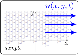
Figure 3: We consider the flow of an electron liquid through a graphene sample that extends over the region $y>0$. The drift velocity is oriented along the $x$-axis. The sample edge at $y=0$ is a source of momentum dissipation.

II.1.1 Nearly specular limit

Under the assumtion that the relevant momentum relaxation at the wall stems from the irregular shape of the boundary, the boundary conditions can be obtained from the scattering behavior of the electronic wave function near a rough surface. Early phenomenological parametrizations of the scattering behavior near such a surface go back to Maxwell Maxwell1867 and Fuchs Fuchs1938 . Here, we follow a more microscopic approach along the lines of Refs. Buchholtz1979 ; Falkovsky1983 .

Let the rough surface be oriented along the $x$-axis and its shape be given by the function $\xi\left(x\right)$ (see Fig. 4).

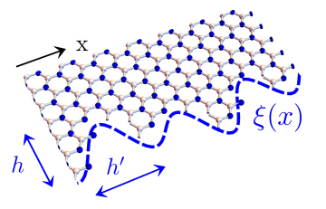
Figure 4: The disordered edge of a graphene sample is described by the function $\xi\left(x\right)$ and characterized by its mean height $h$ and correlation length $h^{\prime}$. Both are much smaller than the thermal wavelenght of the graphene electrons. On average, the edge can be described by the distribution $\overline{\xi\left(x_{1}\right)\xi\left(0\right)}=h^{2}\exp\left(-\frac{x^{2}}{h^{\prime 2}}\right)$.

Before we can address the question of the boundary conditions for the distribution function, we need to know the behavior of the Dirac wave function, i.e. that of low energy excitations, at the sample edge. It was shown in Ref. Akhmerov2008 within a tight-binding approach that for almost any cut through the honeycomb lattice the appropriate boundary condition is, quantitatively very similar to that of the zig-zag edge. The only exception would be an armchair edge that extends without disturbance over a large distance - something wich is unprobable for a disordered edge and is excluded here. This means that the wave function on one sublattice $a=1$ vanishes at the boundary, whereas the wave function on the other sublattice $a=2$ remains undetermined, or vice versa. The valley degrees of freedom are not mixed. To derive the boundary condition for the distribution function $f_{\lambda,\bm{k}}$, it suffices to impose the condition

$$\psi_{a=1}\left(x,y=\xi\left(x\right)\right)=0.$$ (15)

The deviations $\xi\left(x\right)$ must be larger than the interatomic distances, but small compared to the typical wavelength of Dirac electrons at low temperatures. The boundary condition (15) can then be expanded in $\xi\left(x\right)$:

$$\psi_{1}\left(x,0\right)+\xi\left(x\right)\frac{\partial\psi_{1}\left(x,y\right)}{\partial y}\Bigg{|}_{y=0}=0.$$ (16)

We consider elastic scattering at the boundary only, therefore it is usefull to introduce the projection of a wave function onto quasi-free plane-wave states with a given energy $\epsilon$:

$$\psi_{1,\epsilon}\left(\bm{x}\right)=\sum_{\lambda}\int\frac{d^{2}k}{\left(2\pi\right)^{2}}\delta\left(\epsilon-\epsilon_{\lambda,k}\right)\gamma_{\bm{k},\lambda}U_{1,\lambda}\left(\bm{k}\right)e^{i\bm{k}\cdot\bm{r}}.$$ (17)

Here, $\epsilon_{\lambda,k}=\lambda v\hbar k$ is the electron dispersion and $U_{a,\lambda}\left(\bm{k}\right)$ transforms the wavefunctions $\gamma_{\bm{k},\lambda}$ from the band basis into the sublattice basis. $\psi_{\bm{k},a}=\sum_{\lambda}\gamma_{\bm{k},\lambda}U_{a,\lambda}\left(\bm{k}\right)$ is the Bloch function projected onto the sublattice. Inserting $\psi_{1,\epsilon}\left(\bm{x}\right)$ into (16), carrying out the $k_{x}$ integration, and performing a Fourier transform, we obtain to second order in $\xi\left(x\right)$ a relation between the wavefunctions $\gamma_{k_{x},\left|k_{y}\right|,\lambda}$ and $\gamma_{k_{x},-\left|k_{y}\right|,\lambda}$ on the boundary. This relation holds for $\lambda=\pm 1$ separately, because of the elasticity of the scattering process. Then, an average over the edge shapes $\overline{\xi\left(x_{1}\right)\xi\left(x_{2}\right)}$ is taken, so that translation invariance along the edge is restored:

$$\overline{\xi\left(k_{1}\right)\xi\left(k_{2}\right)}=2\pi\delta\left(k_{1}+k_{2}\right)W\left(k_{1}\right).$$ (18)

Thus, $W\left(k\right)$ describes the correlation of the surface roughness. The squared moduli of the wavefunctions are directly related to the kinetic distribution function on the boundary:

$$f_{\bm{k},\lambda}=\left(2\pi v_{k_{x},\lambda}^{y}\right)^{-1}\overline{\left|\gamma_{k_{x},k_{y}\left(\epsilon,k_{x}\right),\lambda}\right|^{2}}.$$ (19)

The prefactor $\left(2\pi v_{k_{x},\lambda}^{y}\right)^{-1}$ stems from a variable change $k_{x},\epsilon\rightarrow\bm{k}$. In this fashion we arrive at the boundary condition

$$f^{>}\left(k_{x},k_{y}\right) = f^{<}\left(k_{x},-k_{y}\right)$$

$$-4f^{<}\left(k_{x},-k_{y}\right)k_{y}\int\frac{dk^{\prime}_{x}}{2\pi}k^{\prime}_{y}W\left(k_{x}-k^{\prime}{}_{x}\right)$$

$$+4k_{y}\int\frac{dk^{\prime}_{x}}{2\pi}k^{\prime}_{y}W\left(k_{x}-k^{\prime}{}_{x}\right)f^{<}\left(k^{\prime}_{x},-k^{\prime}_{y}\right),$$

where $\gtrless$ stands for the sign of the velocity component in the $y$-direction. Except for the matrix elements $U_{a,\lambda}\left(\bm{k}\right)$, which ultimately cancel out, and the fact that two bands $\lambda=\pm 1$ have to be kept track of, the calculation is completely analogous to the one presented by Falkovsky in Falkovsky1983 . The domain of integration in (II.1.1) ranges from $k^{\prime}_{x}=-\epsilon/v$ to $k^{\prime}_{x}=\epsilon/v$ where $k_{y}=\sqrt{\left(\epsilon/v\right)^{2}-k_{x}^{2}}$. Interchanging the sublattice index in Eq. (15) does not alter the result of Eq. (II.1.1).

We assume that the edge correlation function $\overline{\xi\left(x_{1}\right)\xi\left(x_{2}\right)}$ is given by a Gaussian distribution

$$\overline{\xi\left(x_{1}\right)\xi\left(0\right)}=h^{2}e^{-\frac{x^{2}}{h^{\prime 2}}},$$ (21)

where $h$ is the typical amplitude of $\xi(x)$ and $h^{\prime}$ is their correlation length. We then have

$$W\left(k_{x}\right)=\sqrt{\pi}h^{2}h^{\prime}e^{-\frac{1}{4}k_{x}^{2}h^{\prime 2}}.$$ (22)

In graphene at charge neutrality the characteristic energy of excitations is $\epsilon_{T}\sim k_{B}T$. If the lengths $h$, $h^{\prime}$ are of the order of a few interatomic distances, we can safely assume for the thermal wavelength $\lambda_{T}=v\hbar/\epsilon_{T}$ that

$$h^{\prime}\ll\lambda_{T},$$ (23)

and therefore that $W\left(k_{x}\right)$ is a flat function:

$$W\left(k_{x}\right)\approx\sqrt{\pi}h^{2}h^{\prime}.$$ (24)

The presence of the small parameter $h^{2}h^{\prime}/\lambda_{T}^{3}$ is the reason, why our analysis of the slip length in the nearly specular limit is well controlled. The boundary condition (II.1.1) does conserve the number of particles and has essentially the form of the boundary condition proposed by Fuchs Fuchs1938 , where

$$p\left(\bm{k}\right)=1-4k_{y}\int\frac{dk^{\prime}_{x}}{2\pi}k^{\prime}_{y}W\left(k_{x}-k^{\prime}{}_{x}\right)$$ (25)

takes the role of a specularity parameter which depends on the angle of incidence.

II.1.2 Diffuse limit

An alternative boundary condition is valid in the limit of totaly diffuse boundary scattering. Here, it is sufficient to assume that the distribution of electrons departing from the wall does not depend on the particle directions, i.e.

$$f_{\lambda,\bm{k}}^{>}=f_{\lambda}^{>}\left(\left|\bm{k}\right|\right).$$ (26)

Clearly, in such a case all tangential momentum is lost in an electron-wall collision. The diffuse limit is appropriate, if the sample edge is very rough and one makes no assumption on the elasticity of the scattering processes.

II.2 Kinetic equation at a boundary

Next, we determine the electron flow behavior that characterizes the transfer of momentum near the surface within a kinetic theory. Generally, within the Chapman-Enskog approach Chapman1970 ; Cercignani1988 , the bulk kinetic distribution function has the form

$$f\big{|}_{b}=f^{l.e.}-\frac{\partial f^{0}}{\partial\epsilon}\Psi,$$ (27)

where $f^{l.e.}$ is the local equilibrium distribution function, which is found by setting the collision integral to zero, and $f^{0}$ the distribution function for the global equilibrium. For graphene electrons

$$f_{\lambda,\bm{k}}^{l.e.}=\frac{1}{e^{\beta\left(\epsilon_{\lambda,\bm{k}}-\bm{u}\left(\bm{r},t\right)\cdot\bm{k}-\mu\right)}+1}$$ (28)

and $f^{0}$ is the Fermi-Dirac distribution. The inverse temperature $\beta=1/(k_{B}T)$ is not to be confused with the coordinate index $\beta$. $\Psi$ is a non-equilibrium contribution describing the response to shear and other forces. The response to shear forces is characterized by the viscosity $\eta$ of a system, defined via the relation

$$\tau_{\alpha\beta}=-\eta\frac{\partial u_{\alpha}}{\partial x_{\beta}}$$ (29)

between the stress (momentum current) tensor $\tau_{\alpha\beta}=N\hbar v\sum_{\lambda}\int\frac{d^{2}k}{\left(2\pi\right)^{2}}\left(\lambda k_{\alpha}k_{\beta}/k\right)f_{\mathbf{k}\lambda}$ and the gradient of the drift velocity. In the absence of a wall, the kinetic distribution function for graphene at charge neutrality and due to electron-electron Coulomb interaction was calculated in Mueller2009 (the main points are summerized in Appendix B). In the presence of shear forces only, the bulk distribution to leading order in the fine structure constant $\alpha=e^{2}/\left(\epsilon\hbar v\right)$ (not to be confused with the coordinate index $\alpha$) and the drift velocity $\bm{u}$ is given by

$$f_{\lambda,\bm{k}}\big{|}_{b} =f_{\lambda,\bm{k}}^{l.e.}+\beta f_{\lambda,\bm{k}}^{0}\left(1-f_{\lambda,\bm{k}}^{0}\right)\Psi,$$ (30)

where

$$\Psi = \frac{\lambda}{2\sqrt{2}}\left(C_{0}+C_{1}\beta vk\right)I_{\alpha\beta}X_{\alpha\beta}$$

$$X_{\alpha\beta} = \frac{\partial u_{\alpha}}{\partial x_{\beta}}+\frac{\partial u_{\beta}}{\partial x_{\alpha}}-\delta_{\alpha\beta}\nabla\cdot\bm{u}$$

$$I_{\alpha\beta} = \sqrt{2}\left(\frac{k_{\alpha}k_{\beta}}{k^{2}}-\frac{1}{2}\delta_{\alpha\beta}\right).$$ (31)

Here, $C_{0}$ and $C_{1}$ are dimensionless numerical coefficients - the $\psi_{0}$ and $\psi_{1}$ of Appendix B - that are found by solving the kinetic equation Mueller2009 (see Appendix B). $C_{0}$ and $C_{1}$ correspond to the zero modes of the collinear part of the collision integral and are dominant at leading order in the fine structure constant $\alpha$. The expression (30) can be used to determine the viscosity of graphene electrons

$$\eta=N\frac{\left(\pi^{3}C_{0}+27\zeta(3)\pi C_{1}\right)}{48\pi^{2}\beta^{2}v^{2}\hbar}\approx\frac{0.449N}{4\alpha^{2}v^{2}\hbar}\left(k_{B}T\right)^{2},$$ (32)

with $N=4$ being the spin valley degeneracy.

In the presence of the sample edge, we expect corrections of the order $h^{2}h^{\prime}$ to the bulk distribution function stemming from the edge, therefore we make for the distribution function $f_{\lambda,\bm{k}}^{<}\left(y=0\right)$ of particles impinging on the edge the ansatz

$$f_{\lambda,\bm{k}}^{<}\left(y=0\right)=f_{\lambda,\bm{k}}\big{|}_{b}+\mathcal{O}\left(h^{2}h^{\prime}k_{T}^{3}\right)A\left(I_{\alpha\beta}X_{\alpha\beta}\right),$$ (33)

where $A\left(I_{\alpha\beta}X_{\alpha\beta}\right)$ is some function of gradients of the drift velocity $\bm{u}$ and momenta $k^{i}$. As we will show later, this correction contributes to the slip-length only to second order in $h^{2}h^{\prime}$ and we can ignore the contribution $A\left(I_{\alpha\beta}X_{\alpha\beta}\right)$. In other words, one can safely assume that the distribution function of the electrons that move towards the sample edge is governed by the bulk distribution function. Thus, the loss of tangential momentum is described by the boundary condition (II.1.1) and we do not need to make any assumtions on the influence of the boundary on momentum currents. Inserting (33) into (II.1.1) we obtain an expression for $f_{\lambda,\bm{k}}^{>}\left(y=0\right)$. In this way we know the distribution function at the edge $f_{\lambda,\bm{k}}\left(y=0\right)$.

II.3 The slip length

II.3.1 The nearly specular limit

Knowing the functions $f_{\lambda,\bm{k}}^{<}\left(y=0\right)$ and $f_{\lambda,\bm{k}}^{>}\left(y=0\right)$ as a function of $u_{x}\left(y=0\right)$ and $\left.\partial_{y}u_{x}\right|_{y=0}$, we find the hydrodynamic boundary condition with the help of Eq. (14). It is also possible to obtain a boundary condition of the form (3) by avereging over the momentum:

$$\frac{3n_{E}}{2v^{2}}u_{x} = 2N\int_{<}\frac{d^{d}k}{\left(2\pi\right)}k_{x}f_{+,\bm{k}}^{<}\left(y=0\right)$$ (34)

$$+2N\int_{>}\frac{d^{d}k}{\left(2\pi\right)}k_{x}f_{+,\bm{k}}^{>}\left(y=0\right).$$

Note, that the drift velocity is related to the momentum density $\bm{g}_{\bm{k}}=\sum_{\lambda}\int d^{2}k^{\prime}/\left(2\pi\right)^{2}\left(\hbar\bm{k}\right)f_{\lambda,k}$ via $\left(3n_{E}/2v\right)\bm{u}\approx\bm{g}_{\bm{k}}$, where $n_{E}$ is the energy density Briskot2015 . In the nearly specular limit, the two approaches (34) and (14) give the same result. In the diffuse scattering limit the second equation (14) will give the better result, because the additional factor $\sin\left(\varphi\right)$ in the integrands - due to $v_{+,\bm{k}}^{y}$ - gives more weight to contributions from particles with an incidence angle near $\pi/2$. These particles are least influenced by the Knudsen boundary layer - a one mean free path broad region along the sample edge where the distribution function significantly deviates from its bulk values. Therefore our assumption that the loss of tangential momentum is determined directly at the wall, by the boundary condition (II.1.1), is appropriate here.

Performing the average, we see that only those parts of $f_{\lambda,\bm{k}}\left(y=0\right)$ contribute, which are proportional to $\cos\left(\varphi\right)$. Therefore, for a flat $W\left(k_{x}\right)$, the last right hand side term of (II.1.1) does not contribute to the momentum current average (14). After performing the integrations we have from (14)

$$0=-\left(\frac{h^{2}h^{\prime}}{\lambda_{T}^{3}}\right)Au_{x}+\eta\frac{\partial u_{x}}{\partial y}-\left(\frac{h^{2}h^{\prime}}{\lambda_{T}^{3}}\right)B\frac{\partial u_{x}}{\partial y},$$ (35)

where we have defined the thermal wavelength $\lambda_{T}=\beta v\hbar$ and $A=\frac{N31\pi^{11/2}}{672\beta^{3}v^{3}\hbar^{2}}.$ It is again clear, that $h^{2}h^{\prime}/\lambda_{T}^{3}$ plays the role of a small dimensionless parameter. Physically, the presence of the small parameter $h^{2}h^{\prime}/\lambda_{T}^{3}$ shows that the edge behaves as if it was smooth, if its roughness is on average much smaller than the typical wavelength of scattered electrons. Solving for $u_{x}$, we write the above equation in the form of (3). To leading order in $h^{2}h^{\prime}/\lambda_{T}^{3}$ the slip length is given by

$$\zeta=\left(\frac{\lambda_{T}^{3}}{h^{2}h^{\prime}}\right)\chi\approx 0.008\left(\frac{\lambda_{T}^{3}}{h^{2}h^{\prime}}\right)l_{ee},$$ (36)

where $\chi=\frac{672\beta^{3}v^{3}\hbar^{2}}{N31\pi^{11/2}}\eta$. We used $l_{ee}=v\hbar/\left(\kappa_{1}\alpha^{2}k_{B}T\right)$ for the mean free path due to electron scattering with numerical coefficient $\kappa_{1}=1.950$ (see Appendix B).

II.3.2 The diffuse limit

The overall procedure to find the boundary condition in the diffuse limit is analogous to the nearly specular case. Due to the condition (26) only impinging particles with a negative velocity contribute to the average over the momentum current. In distinction to the nearly specular case however, we do not have a small parameter and therefore assume that the incident electron’s behavior is described by the bulk distribution function up to right at the edge. In the theory of classical gases, this assumption leads to the famous Maxwell boundary condition Maxwell1867 for rarified gas flow (see also Kramers1949 ; Kennard1938 ). The momentum current averaged over the distribution function given in Eq. (26) yields

$$\zeta=\frac{\pi^{2}\beta^{3}v^{3}\hbar^{2}}{3N\zeta(3)}\eta \approx 0.6l_{ee}.$$ (37)

Again, we used the electron mean free path $l_{ee}=v\hbar/\left(\kappa_{1}\alpha^{2}k_{B}T\right)$.

II.3.3 Discussion

In the diffuse limit, as well as in the nearly specular limit the slip length $\zeta$ approaches infinity as $T\rightarrow 0$. While in the diffusive limit $\zeta\sim T^{-1}\ln^{3}\left(T_{\Lambda}/T\right)$ with $T_{\Lambda}=\Lambda/k_{B}$, in the nearly specular limit holds $\zeta\sim T^{-4}\ln^{6}\left(T_{\Lambda}/T\right)$, showing clearly that the mechanism of scattering on a rough boundary is ineffective for electrons with large wavelength. The slip lengths as functions of temperature are shown in Fig. 5.

Figure 5: The figure shows the temperature dependence of the slip length $\zeta$ for a) diffuse scattering at the boundary for graphene at charge neutrality (continuous line) and at finite chemical potential (dashed line) and b) scattering at a microscopically rough edge with a typical roughness of $h=h^{\prime}=250\,\textrm{\AA}$ for graphene at charge neutrality. With decreasing temperature, $\zeta$ grows as $T^{-4}\ln^{6}\left(T_{\Lambda}/T\right)$ in the nearly specular and as $T^{-1}\ln\left(T_{\Lambda}/T\right)$ in the diffuse limits at charge neutrality. Away from charge neutrality the slip length behaves as $\zeta\sim T^{-2}/\ln\left(\epsilon_{F}/T\right)$ in both limits, but is parametrically larger in the nearly specular case.

In the renormalization of the velocity $v_{0}\rightarrow v=v_{0}\left(1+\alpha\ln\left(\Lambda/k_{B}T\right)\right)$ and the coupling constant $\alpha\rightarrow\alpha_{r}=e^{2}/(4\pi\epsilon\hbar v)$ we used a cut-off of $\Lambda\sim 1\,\textrm{eV}$. Also, we assumed a permittivity $\varepsilon=5\varepsilon_{0}$. Our small parameter for the nearly specular limit $h/\lambda_{T}$ remains, below $100\,\textrm{K}$, small up to an $h\approx 250\,\textrm{\AA}$ (where it is $\approx 1/5$ at $100\,\textrm{K}$).

In the diffusive limit, for the same parameter values as above, $\zeta$ ranges from $100\,\upmu\textrm{m}$ at $1\text{K}$ to $0.4\,\upmu\textrm{m}$ at $100\textrm{K}$. In the nearly specular limit, for a small roughness of the order of $h=h^{\prime}=10\,\textrm{\AA}$, $\zeta$ is comparable to the length of the Trans-Siberian Railway at $T=1\,\mbox{K}$ and ranges to $1\,\textrm{mm}$ at $T=100\,\text{K}$. For a fairly rough edge of $h=h^{\prime}=250\,\textrm{\AA}$ we have at $1\,\text{K}$ $\zeta=3.5\,\textrm{km}$ and at $T=100\,\text{K}$ the slip length $\zeta\approx 0.6\,\upmu\textrm{m}$ approaches the diffuse limit. Such large values for $\zeta$ imply that one can effectively use no-stress boundary conditions.

We finally note, that the specularity of different kinds of edges of different materials is well studied Tsoi1999 . For oxygen-plasma-etched graphene specifically, values of 0.2 to 0.5 were reported for the specularity parameter $q$ (which gives the probability that a single scattering event at the edge is specular) Taychatanapat2013 . Therefore, under these particular conditions the slip lengths are expected to lie somewhere between the nearly specular and the diffuse scattering limits.

II.4 Fermi liquids and graphene away from charge neutrality

Our derivation of boundary conditions for the hydrodynamic flow of a Dirac liquid can also be applied to the Fermi liquids, which includes graphene far away from charge neutrality. Let us again assume that the $y$-axis is orthogonal to the boundary of the sample, that the Fermi liquid is contained in the region $y>0$, and that the flow is tangential to the boundary.

Following Abrikosov1959 , we write the distribution function of quasiparticles as

$$f=f_{0}\left(\epsilon\right)-\frac{\partial f_{0}}{\partial\epsilon_{0}}\Psi.$$ (38)

Here, $\epsilon$ is the full quasiparticle energy which itself depends on the occupation numbers and $\epsilon_{0}=v_{F}\hbar\left(k-k_{F}\right)+\epsilon_{F}$. The funtion $\Psi$ describes the response to gradients of the drift velocity $\bm{u}$. In the considered geometry, it can be parametrized as

$$\Psi=+q\left(p\right)p_{x}\frac{\partial\epsilon}{\partial p_{y}}\frac{\partial u_{x}}{\partial y}.$$ (39)

The stress tensor is given by

$$\tau_{xy}=\int\frac{d^{d}k}{\left(2\pi\right)^{d}}\left(p_{x}v_{F}^{y}\right)\frac{\partial f_{0}}{\partial\epsilon_{0}}\Psi.$$ (40)

Comparing to the relation $\tau_{xy}=-\eta\partial u_{x}/\partial y$, we find for the viscosity the expression

$$\eta=-\int\frac{d^{d}k}{\left(2\pi\right)^{d}}\left(p_{x}v_{F}^{y}\right)^{2}q\left(p\right)\frac{\partial f_{0}}{\partial\epsilon_{0}}.$$ (41)

For $d=3$ we then have

$$\eta=\frac{2}{15}v_{F}^{2}\rho_{F}\epsilon_{F}m^{*}\tau$$ (42)

and for $d=2$

$$\eta=\frac{1}{4}v_{F}^{2}\rho_{F}\epsilon_{F}m^{*}\tau,$$ (43)

where $\rho_{F}$ is the density of states at the Fermi surface and

$$\tau=\int_{-\infty}^{\infty}dx\frac{q\left(x\right)}{\left(2\cosh\left(\frac{x}{2}\right)\right)^{2}},$$ (44)

with the dimensionless integration variable $x=\epsilon-\epsilon_{F}/\left(k_{B}T\right)$. The quantity $q\left(x\right)$ must be found by solving the linearized kinetic equation.

For $d=3$ it was shown in Abrikosov1959 that $q\left(x\right)$ can be assumed constant. This yields that the leading temperature dependence at $\epsilon_{F}\gg k_{B}T$ is $\eta\propto q\propto T^{-2}$. where $v_{F}$ is the Fermi velocity. The detailed expressions for the kinetic distribution function and viscosity can be found in Abrikosov1959 . Compared to the case of graphene, the boundary condition (II.1.1) holds as it is, except for the fact that the integrations have to be performed over a two-dimensional surface and only the $\lambda=+1$ part is relevant. Furthermore $N=2$ due to the spin degeneracy.

In the nearly specular limit the role of the thermal wavelength $\lambda_{T}$ is played by the Fermi-wavevector $k_{F}$, as it determines the characteristic wavelength of the exitations. The slip length as derived from (14) to leading order in the parameter $1/h^{2}h^{\prime 2}k_{F}^{4}$ and to leading order in temperature is

$$\zeta=\left(\frac{1}{h^{2}h^{\prime 2}k_{F}^{4}}\right)\chi\approx\left(\frac{1}{h^{2}h^{\prime 2}k_{F}^{4}}\right)3l_{ee},$$ (45)

where $\chi=\frac{45\pi^{2}}{k_{F}^{4}\hbar}\eta$. In the diffuse scattering limit, we find

$$\zeta=\frac{8\pi^{2}}{k_{F}^{4}\hbar}\eta\approx 0.5l_{ee}.$$ (46)

We used $l_{ee}=v_{F}\tau$ and $\rho_{F}=m^{*}k_{F}/\left(\hbar\pi\right)^{2}$. The temperature dependence of the slip length in the diffuse scattering limit as well as in the nearly specular limit is $\zeta\sim 1/T^{2}$.

Poiseuille type flow was observed in the delafossite PdCoO₂ Moll2016 . The same publication reports a viscosity of up to $6\cdot 10^{-3}\,\textrm{kg}/(\textrm{ms})$. With the help of Eq. (46) we find a slip length of $\zeta=0.45\,\upmu\textrm{m}$. This length is indeed small compared to the sample widths of up to $60\,\upmu\textrm{m}$, meaning that the slip velocity at the boundaries is negligable, which, again, is fully consistent with the observed Poiseuille behavior. A comparable value for the electron viscosity and Poiseuille type flow in the Weyl material WP₂ was reported in Gooth2017 . The sample widths exeeded the slip length as given by (46) and the observations were consistent with our theory. A typical Fermi liquid, however, is expected to have a higher viscosity and a larger slip length.

For $d=2$ we can crudely estimate the time $\tau$ by the quasiparticle lifetime $\tau_{qp}$, which is known to be logarithmically suppresed at low temperatures compared to the $d=3$ result Hodges1971 . From the Refs. Reizer1997 ; Zheng1996 ; Menashe1996 we expect

$$\tau_{qp}=A\frac{\epsilon_{F}\hbar}{\left(k_{B}T\right)^{2}}\frac{1}{\ln\left(\frac{\epsilon_{F}}{k_{B}T}\right)},$$ (47)

where $A$ is a coefficient of the order of unity. From (14) we obtain in the nearly specular limit

$$\zeta=\left(\frac{\hbar^{3}v_{F}^{3}/\epsilon_{F}^{3}}{h^{2}h^{\prime}}\right)\chi\approx\left(\frac{1}{h^{2}h^{\prime}k_{F}^{3}}\right)1.1l_{ee},$$ (48)

with $\chi=\frac{2}{\sqrt{\pi}}v_{F}\tau$, and in the diffuse limit $\zeta=\frac{3\pi}{8}v_{F}\tau$, so that

$$\zeta\approx 1.2l_{ee}.$$ (49)

These results also apply to graphene at finite chemical potential. The viscosity of graphene can then be written $\eta=\frac{1}{8}\rho_{F}^{G}\mu^{2}\tau$. Using the quasiparticle lifetime (47) with $A=1$ to estimate $\tau$, the slip lengths for graphene at $\mu\gg k_{B}T$ in the diffusive limit are larger than for graphene at charge neutrality. For $\mu=0.25\textrm{eV}$, they range from $0.8\,\upmu\textrm{m}$ at $100\,\textrm{K}$ to $3\textrm{mm}$ at $1\,\textrm{K}$ (see Fig 5). The reason for the larger slip lengths is the $1/\left(T^{2}\ln\left(\epsilon_{F}/k_{B}T\right)\right)$ temperature dependence of $\tau$. In the nearly specular case, the small parameter $\hbar^{3}v_{F}^{3}/\left(h^{2}h^{\prime}\epsilon_{F}^{3}\right)=1/(h^{2}h^{\prime}k_{F}^{3})$ does not depend on the thermal wavelength $\lambda_{T}$, but instead on the wavelength at the Fermi surface. Since the edge roughness $h$ has to be compared to $k_{F}^{-1}\ll\lambda_{T}$, the diffusive limit - giving the minimal $\zeta$, since all tangential momentum is lost - can be saturated for much smaller $h$ than at charge neutrality. Still, $\zeta$ as given by (49) is large enough to justify no-stress conditions for most geometries.

Our result explains the findings of Bandurin , where in graphene samples with widths up to $4\,\upmu\textrm{m}$ no Gurzhi effect was observed up to $100\,\textrm{K}$ and strengthen the author’s conjecture that the small deviation of the resistivity curves at about $100\,\textrm{K}$ indeed stems from a small hydrodynamic contribution due to the Gurzhi effect (supplement to Bandurin ). The reason is that at about $100\,\textrm{K}$ the slip length drops below $1\,\upmu\textrm{m}$ and becomes smaller than the sample width.

Let us finally note that the diffusive boundary condition gives the smallest possible slip length and is a “worst case scenario” in the sense that all tangential momentum is lost; be it due to elastic or inelastic scattering. While the nearly specular scattering limit deals with the opposite scenario and elastic scattering only, one could imagine that considering larger and larger roughnesses $h$, the slip length would saturate at some value $\zeta_{min}$, which is close to the slip length of the diffusive scattering limit.

III Comparison to known results

Most calculations of slip in quantum fluids Levinson1977 ; HJensen1980 ; Einzel1984 ; Einzel1990 ; Einzel1997 model interactions by a momentum conserving relaxation time ansatz, similar to the one used in the Bhatnagar-Gross-Krook equation Bhatnagar1954 . The collision integral is replaced by the term $-g/\tau$, where $g$ is the deviation of the distribution function not from the global, but from the local equilibrium:

$$g=f-f^{l.e.}.$$ (50)

Within this approach, it was shown in HJensen1980 for a diffusely scattering boundary that the slip length determined in analogy to the Maxwell slip length (see Maxwell1867 ; Kramers1949 ; Kennard1938 ), i. e. by assuming the validity of the bulk distribution function for ingoing particles up to the boundary, gives a lower bound on the slip length $\zeta$ as calculated within the Bhatnagar-Gross-Krook-like approach. For completeness, we want to summerize the logic of HJensen1980 briefly and discuss how it relates to our results.

The analysis applies to two or three dimsensions and to arbitrary dispersion relations. Therefore we will not specify dimensionality and dispersion until the end. Let the $y$-axis be orthogonal to the sample boundary and the quantum fluid be contained in the volume $y>0$. The kinetic equation becomes

$$v_{y}\frac{\partial g}{\partial y}-v_{y}p_{x}\frac{\partial f^{0}}{\partial\epsilon}\frac{\partial u_{x}}{\partial y}=-\frac{g}{\tau}$$ (51)

and is a first order differential equation for $g$ which is easily solved as soon as the appropriate boundary conditions are formulated. The idea is to describe the physics of the Knudsen layer right at the boundary, where the system is not in local equilibrium, but significantly influenced by the scattering of particles at the sample edge. At $y\rightarrow\infty$ the Knudsen layer ends and the system enters the hydrodynamic regime described by the Navier-Stokes equations. Therefor the gradient of the drift velocity $u^{\prime}=\partial u_{x}/\partial y$ approaches a finite value $u^{\prime}\left(\infty\right)$ and it holds

$$g\left(\infty\right)=\tau v_{y}p_{x}\frac{\partial f^{0}}{\partial\epsilon}u^{\prime}\left(\infty\right).$$ (52)

Figure 6: The Knudsen-layer - an approximately one mean free path broad region along the momentum dissipating boundary of a liquid - is depicted. The fluid behavior in the Knudsen layer is not described by hydrodynamic equations. The reasoning behind the introduction of the slip length $\zeta$ is to pass the information about Knudsen layer physics to the hydrodynamic equations. While the drift velocity $\bm{u}\left(y\right)$ in the Knudsen layer is smaller than the surface velocity $\bm{u}_{S}$ of Eq. (3), the gradient $\partial u_{x}\left(y\right)/\partial y$ approaches the value prescribed by $u_{S}=\partial u/\partial y|_{S}$ at the very end of the layer. Extrapolating this gradient up to zero velocity one obtains the slip length $\zeta$.

In addition, one assumes that $f\left(0\right)=f^{0}$ for positive velocities $v_{y}>0$, which is equivalent to

$$g\left(0\right)=p_{x}u\left(0\right)\frac{\partial f^{0}}{\partial\epsilon},$$ (53)

again holding for $v_{y}>0$. With these boundary conditions, (51) is solved by

$$g_{v_{y}>0} =p_{x}u\left(0\right)\frac{\partial f^{0}}{\partial\epsilon}e^{-\frac{y}{\tau v_{y}}}+\int_{0}^{y}dy^{\prime}p_{x}u^{\prime}\left(y^{\prime}\right)\frac{\partial f^{0}}{\partial\epsilon}e^{-\frac{\left|y^{\prime}-y\right|}{\tau v_{y}}}$$

$$g_{v_{y}<0} =-\int_{y}^{\infty}dy^{\prime}p_{x}u^{\prime}\left(y^{\prime}\right)\frac{\partial f^{0}}{\partial\epsilon}e^{\frac{\left|y^{\prime}-y\right|}{\tau v_{y}}}.$$ (54)

The influx current of tangential momentum into the Knudsen layer is given by $-\eta u^{\prime}$$\left(\infty\right)$. The authors of Ref HJensen1980 further assume that this current is constant in the whole Knudsen layer, and only at the boundary is it converted into a tangential flow that creates a velocity slip. In our treatment of the kinetic distribution at the nearly specular boundary in section II.2, where we showed that the variation of the tangential momentum current gives a contribution subleading in the small parameter $h^{2}L/\lambda_{T}^{3}$, we explicitly saw that this assumption holds. If it holds in the totally diffuse case as well, we can write

$$-\eta u^{\prime}\left(\infty\right) =\int_{>}\frac{d^{d}k}{\left(2\pi\right)^{d}}v_{y}p_{x}^{2}u\left(0\right)\frac{\partial f^{0}}{\partial\epsilon}e^{-\frac{y}{\tau v_{y}}}$$

$$+\int_{>}\frac{d^{d}k}{\left(2\pi\right)^{d}}v_{y}p_{x}^{2}\int_{0}^{y}dy^{\prime}u^{\prime}\left(y^{\prime}\right)\frac{\partial f^{0}}{\partial\epsilon}e^{-\frac{\left|y^{\prime}-y\right|}{\tau v_{y}}}$$

$$-\int_{<}\frac{d^{d}k}{\left(2\pi\right)^{d}}\int_{y}^{\infty}dy^{\prime}v_{y}p_{x}^{2}u^{\prime}\left(y^{\prime}\right)\frac{\partial f^{0}}{\partial\epsilon}e^{\frac{\left|y^{\prime}-y\right|}{\tau v_{y}}}.$$ (55)

Eq. (55) is an integral equation for $u^{\prime}\left(y\right)$. Reference HJensen1980 develops a method to extract from Eq. (55) information about the slip length, without seeking an explicit solution: First, the function $L_{n}\left(y\right)$ is introduced such that

$$L_{n}\left(y\right)=g_{N}\int_{>}\frac{d^{d}k}{\left(2\pi\right)^{d}}v_{y}p_{x}^{2}\left(\tau v_{y}\right)^{n-1}\left(-\frac{\partial f^{0}}{\partial\epsilon}\right)e^{-\frac{y}{\tau v_{y}}}.$$ (56)

$g_{N}$ accounts for additional degeneracies. In the case of graphene, a factor of $g_{N}=2N$ in front of the integral will account for excitations with positive and negative energies and the spin-valley degeneracy. The viscosity can be expressed as

$$\eta=\tau\int\frac{d^{d}k}{\left(2\pi\right)^{d}}v_{y}^{2}p_{x}^{2}\left(-\frac{\partial f^{0}}{\partial\epsilon}\right)=2L_{2}\left(0\right).$$ (57)

Definig the function $\Psi\left(z\right)$ via the equation $u^{\prime}\left(z\right)=u^{\prime}\left(\infty\right)$$\left(1+\Psi\left(z\right)\right)$ and introducing $y_{0}=u\left(0\right)/u^{\prime}\left(\infty\right)$, one can reduce Eq. (55) to

$$z_{0}L_{1}\left(z\right)-L_{2}\left(z\right)=-\int_{0}^{\infty}dz^{\prime}\Psi\left(z^{\prime}\right)L_{1}\left(\left|z-z^{\prime}\right|\right).$$ (58)

Notice that since the drift velocity is expected to drop compared to the hydrodynamic boundary value $u_{S}=u^{\prime}\left(\infty\right)\zeta$, the function $\Psi\left(z\right)$ is expected to be positive everywhere and to vanish for $y\rightarrow\infty$. For the slip length $\zeta$ the following holds (see Fig. 6):

$$u_{S}=u^{\prime}\left(\infty\right)\zeta =u\left(0\right)+\int_{0}^{\infty}u^{\prime}\left(z^{\prime}\right)-u^{\prime}\left(\infty\right)dy^{\prime}$$

$$\zeta =y_{0}+\int_{0}^{\infty}\Psi\left(y^{\prime}\right)dy^{\prime}.$$ (59)

Together with (58) this yields

$$\zeta L_{1}\left(y\right)-L_{2}\left(y\right)=-\int_{0}^{\infty}dy^{\prime}\Psi\left(y^{\prime}\right)\left(L_{2}\left(\left|y-y^{\prime}\right|\right)-L_{1}\left(y\right)\right).$$ (60)

One property of the functions $L_{n}\left(y\right)$ is $dL_{n}\left(y\right)/dy=-L_{n-1}\left(y\right)$. Using this relationship, the above equation can be integrated over the region $y>0$ to yield

$$\zeta L_{2}\left(0\right)-L_{3}\left(0\right)=\int_{0}^{\infty}dy^{\prime}\Psi\left(y^{\prime}\right)\left(L_{2}\left(y^{\prime}\right)-L_{2}\left(0\right)\right).$$ (61)

Noticing that $L_{n}\left(y>0\right)<L_{n}\left(0\right)$ and remembering that $\Psi\left(z\right)$ is positive one obtains from (60)

$$\zeta>\frac{L_{2}\left(0\right)}{L_{1}\left(0\right)}$$ (62)

and from (61)

$$\zeta<\frac{L_{3}\left(0\right)}{L_{2}\left(0\right)}.$$ (63)

The equations (62) and (63) consitute a lower and an upper bound on the slip length, which are typically not too far apart and therefore give a good estimate for $\zeta$. The lower bound can even be improved with the help of the inequality $L_{n+1}L_{n-1}>L_{n}^{2}$: Realizing that $d/dy\left(L_{n}\left(y\right)/L_{n+1}\left(y\right)\right)=\left(L_{n}^{2}-L_{n+1}L_{n-1}\right)/L_{n+1}^{\text{2}}<0$, we have $L_{n}\left(y\right)/L_{n}\left(0\right)>L_{n-1}\left(y\right)/L_{n-1}\left(0\right)$. The combination of equations (60) and (61) then yields

$$2\zeta-\frac{L_{2}\left(0\right)}{L_{1}\left(0\right)}-\frac{L_{3}\left(0\right)}{L_{2}\left(0\right)}=\int_{0}^{\infty}dy^{\prime}\Psi\left(y^{\prime}\right)\left(\frac{L_{2}\left(y^{\prime}\right)}{L_{2}\left(0\right)}-\frac{L_{1}\left(y^{\prime}\right)}{L_{1}\left(0\right)}\right)$$ (64)

and

$$\zeta>\frac{1}{2}\left(\frac{L_{2}\left(0\right)}{L_{1}\left(0\right)}+\frac{L_{3}\left(0\right)}{L_{2}\left(0\right)}\right).$$ (65)

As realized by the authors of HJensen1980 , the lower bound (62) is equivalent to the slip length of the Maxwell approach. Remembering the general form of the distribution function (27) one easily sees that in the case of diffuse scattering, and assuming that particles at the boundary are described by the bulk distribution, Eq. (14) reads

$$0=-\frac{1}{2}\eta\frac{\partial u_{x}}{\partial y}+\int\frac{d^{d}k}{\left(2\pi\right)}v_{y}p_{x}^{2}u\left(0\right)\left(-\frac{\partial f^{0}}{\partial\epsilon}\right),$$ (66)

where we have ommited the summation over the two graphene bands. Approximating $\zeta_{lower}=u\left(0\right)/\left(\partial u_{x}/\partial y\right)$ (for the exact slip length we need to replace $u\left(0\right)$ by $u_{S}$), one obtains

$$\zeta_{lower}=\frac{\eta/2}{\int\frac{d^{d}k}{\left(2\pi\right)}v_{y}p_{x}^{2}\left(-\frac{\partial f^{0}}{\partial\epsilon}\right)}=\frac{L_{2}\left(0\right)}{L_{1}\left(0\right)},$$ (67)

which is the lower bound (62) and is, of course, identical to our result of Eq. (37). For graphene, the upper bound (63) and the lower bound are very close: $\zeta_{upper}\approx 1.15\zeta_{lower}$. A comparison of the slip length for the classical kinetic gas given by (65) and (63) with exact and numerical results was performed in HJensen1980 . The authors report a deviation of less than 1%. For completeness, we note that the $\zeta$ obtained from Eq. (34) is equivalent to the lower bound set by $\zeta>L_{1}\left(0\right)/L_{0}\left(0\right)$, which is worse than the lower bound (62).

IV Flow through a strip with a circular obstacle

If the slip length of an electron liquid $\zeta$ is much larger than the typical sample size, it is appropriate to use the no-stress boundary condition of Eq. (2) to model the interaction of the liquid with the wall. If this condition is applied, the conductivity of a clean sample with a Poiseuille geometry is infinite, as is clear from Eq. (5). However, if viscous shear forces act somewhere in the sample, the conductivity becomes finite. This can be used to identify hydrodynamic flow, even when the Gurzhi effect should not be observable at large $\zeta$. Viscous shear forces arise, for example, if the fluid has to bypass an impenetrable obstacle that is put somewhere in the sample. As an illustration, we consider a graphene strip that is infinitely extended in the $x$-direction and goes from $y=-w/2$ to $y=w/2$. The obstacle shall be a disk of radius $a$ placed at the origin of the coordinate system. No-stress boundary conditions shall apply at the interface of obstacle and liquid as well as at $y=\pm w/2$. We calculate the pressure difference that arises due to viscous shear forces between the ends of the strip at $x=-\infty$ and $x=\infty$. In what follows, graphene at charge neutrality is considered but the calculation can be readily modified to suit the Fermi liquid case. In the former case the flow should be probed using thermal transport, while it is given by the electrical current in the latter case.

The full Navier-Stokes equation for graphene electrons reads Mueller2009 ; Briskot2015

$$\frac{\tilde{w}}{v^{2}}\left(\partial_{t}\bm{u}+\left(\bm{u}\cdot\nabla\right)\bm{u}\right)+\nabla p+\frac{\partial_{t}p}{v^{2}}\bm{u}-\eta\nabla^{2}\bm{u}=0.$$ (68)

$\tilde{w}$ is the enthalpy density $\tilde{w}=\frac{3n_{E}/2}{2+\left|\bm{u}\right|/v}\approx\tilde{w}_{0}=\frac{3}{2}n_{E}$. To begin with, we consider a liquid which is not bounded at $y=w/2$. As is well known Batchelor ; Lucas2017 , in two dimensions the flow around a circular obstacle exhibits Stokes’ paradox: the flux $\bm{u}$ is not a linear function of $\nabla p$ for small $\nabla p$. The usual way to circumvent this problem is to use Oseen’s equation Batchelor in which the flow $\bm{u}$ is linearized around a spatially constant flow $\bm{U}\propto\hat{\bm{e}}_{x}$. The full flow $\bm{u}$ is then written

$$\bm{u}=\bm{U}+\bm{q},$$ (69)

and the linearized Navier-Stokes equation reads

$$\frac{\tilde{w}_{0}}{v^{2}}\left(\bm{U}\cdot\nabla\right)\bm{q}+\nabla p-\eta\nabla^{2}\bm{q}=0.$$ (70)

In Appendix C we give the general solution to Eq. (70) following the analysis of Ref. Tomotika1950 . We also calculate the flow around the obstacle for an arbitrary $\zeta$ on an infinite domain. If the flow is not confined to the strip, the pressure induced by the obstacle vanishes at infinity, where $p\sim 1/r$. If, however, the flow is bounded at $y=\pm w/2$, the obstacle does induce a pressure difference along the strip. The boundary conditions imposed on the electron flow by the two walls at $y=\pm w/2$ are

$$q_{y}\left(y=\pm w/2\right) = 0$$

$$\frac{\partial q_{x}\left(y=\pm w/2\right)}{\partial y} = 0.$$ (71)

These boundary conditions can be implemented using the method of images, known from electrostatics. The expression

$$\bm{q}_{tot} =\sum_{j=-\infty}^{\infty}\bm{q}\left(x,y+jw\right),$$ (72)

with $\bm{q}\left(x,y\right)$ being the infinite domain solution obtained in Eq. (C.1)-(C.9), does satisfy Eq. (70) everywhere inside the strip and matches the conditions of Eq. (71). It corresponds to infinitely many image fields placed along the $y$-axis, symmetrically to the original obstacle at $y=0$ (see Fig. 7). The solution $\bm{q}_{tot}$ is only approximate, since the boundary condition at the surface of the obstacle is not matched exactly. It is matched, however, at $r=a$ and $y=0$. Therefore, the error is of order $\sim\frac{a}{w}$ , i. e. small, if the obstacle is small compared to the width of the strip.

Figure 7: The method of images can be used to solve Eq. (70) for a strip-like sample geometry with a circular obstacle. The sample and the electron flow are drawn in color, the image fields are shown in light grey. Infinitely many image solutions must be placed symmetrically around the obstacle in the middle of the sample.

The pressure distribution along the sample can then be calculated from the function

$$\phi_{j}=\phi\left(x,y+jw\right),$$ (73)

which solves the Laplace equation and is defined in Eq. (C.3). The pressure generated by every single image field is $p\left(x,y+jm\right)=U\left(\tilde{w}_{0}/v^{2}\right)\partial\phi_{j}/\partial x$ (for details see Appednix C and Ref Tomotika1950 ). The total pressure at $y=0$ is

$$p_{tot} = \sum_{j=-\infty}^{j=\infty}p\left(x,jm\right)$$ (74)

$$= \frac{\pi A_{0}U^{2}}{w}\frac{\tilde{w_{0}}}{v^{2}}\coth\left(\frac{\pi x}{w}\right)$$

$$+\text{sgn}(x)\frac{\pi^{2}A_{1}U^{2}}{w^{2}}\frac{\tilde{w_{0}}}{v^{2}}\textrm{sinh}\left(\frac{\pi x}{w}\right)^{-2}.$$

The constants $A_{0}$ and $A_{1}$ are given in Eqs. (C.7) and (C.8). While the pressure of any single image field $p\left(x,jm\right)$ vanishes for $x\rightarrow\pm\infty$, the sum over all image fields remains finite. The pressure difference across the sample is then

$$\Delta p=p_{tot}\left(x\rightarrow\infty\right)-p_{tot}\left(x\rightarrow-\infty\right)=2\frac{\pi A_{0}U^{2}}{w}\frac{\tilde{w_{0}}}{v^{2}}.$$ (75)

Using Eqs. (C.7), (C.9) and expanding $B_{0}$ for small $U$ (small Reynolds numbers), as well as taking the limit $\zeta\rightarrow\infty$ for the slip length at the obstacle, we obtain

$$\Delta p=-\frac{8\pi U}{3-2\left(\log\left(\frac{aU}{4\nu}\right)+\gamma\right)}\frac{\tilde{w_{0}}}{v^{2}}\frac{\nu}{w}.$$ (76)

$\nu$ is the kinematic viscosity $\nu=\left(v^{2}/\tilde{w}_{0}\right)\eta$. As expected, the pressure arising due to a small flow velocity $U$ cannot be linearized, which is a manifestation of Stoke’s paradox. We want to link this result to an experimental setup in which a heat flow through the sample will induce a temperature difference. With the help of Eq. (9) we can rewrite the pressure difference as a temperature difference. The flow velocity $U$ is connected to the heat current density through the formula Briskot2015

$$\bm{j}_{E}=\frac{3n_{E}\bm{U}}{2+U^{2}/v^{2}}\approx\frac{3}{2}n_{E}\bm{U}.$$ (77)

With the total energy current being $I_{E}=j_{E}w$ we can write for Eq. (76)

$$\left|\Delta T\right|=\frac{16\pi I_{E}\eta/\left(n_{E}w^{2}s\right)}{9-6\left(\log\left(\frac{1}{9}\frac{I_{E}a}{v^{2}\eta w}\right)+\gamma\right)}.$$ (78)

$\gamma\approx 0.58$ is the Euler constant. This result can be used to determine the viscosity $\eta$. The entropy density is given by Mueller2009

$$s=N\frac{9\zeta\left(3\right)}{\pi}k_{B}\frac{\left(k_{B}T\right)^{2}}{\hbar^{2}v^{2}}.$$

Fig. 8 shows the dependece of the induced temperature difference on the heat current through a $10\,\upmu\textrm{m}$ wide graphene sample at $50\,\textrm{K}$ for an obstacle of radius $a=1\,\upmu\textrm{m}$. The dependence of the temperature difference $\left|\Delta T\right|$ on the radius $a$ is shown in Fig. 9. The scaling behavior of the current with $a$ and $w$ is non-trivial due to the presence of a third length scale $\nu/U$. Since no momentum is dissipated at the sample boundaries the temperature difference along the sample, far enough from the disc, does not depend on the length of the sample. The temperature difference is induced in the region near the disc only.

Figure 8: Temperature difference induced by a heat current $I_{E}$ through a $10\,\upmu\textrm{m}$ wide strip of charge neutral graphene at $50\,\textrm{K}$ with a circular obstace of radius $1\,\upmu\textrm{m}$ at the center of the strip (see Fig. 7). At a heat current of $0.1\upmu\textrm{m}$ the Reynolds number is $\sim 0.74$, approaching unity.

Figure 9: Temperature difference for a fixed heat current of $I_{E}=0.5\upmu\textrm{W}$ through a $10\,\upmu\textrm{m}$ wide graphene channel at $50K$ as a function of the obstacle radius $a$.

V Conclusions

Hydrodynamic flow sensitively depends on the nature of the boundary conditions for the velocity flow field. These boundary conditions can efficiently be characterized by the slip length $\zeta$ introduced in Eq. (3). In order to obtain a quantitative understanding of the slip length in electron fluids, we have derived the slip lengths at different kinds of edges for Dirac and Fermi liquids. We found that for viscous electronic flow the slip length can always be written in the form

$$\zeta=f\left(\kappa\right)l_{ee}$$ (79)

with dimensionless ratio $\kappa=h^{2}h^{\prime d-1}/\lambda^{d+1}$ . $\kappa$ depends on the two length scales $h$ and $h^{\prime}$ that characterize the interface scattering and the electron wavelength $\lambda$, respectively. For graphene at the neutrality point, the latter is strongly temperature dependent ($\lambda=\hbar v/(k_{{\rm B}}T)$), while it corresponds to the Fermi wave length in the case of Fermi liquids ($\lambda=1/k_{{\rm F}}$). The dimensionless function $f\left(\kappa\right)$ diverges for small $\kappa$: $f\left(\kappa\ll 1\right)=f_{0}/\kappa$, while it approaches a constant for strong interface scattering: $f\left(\kappa\rightarrow\infty\right)\rightarrow f_{\infty}$. We determined $f_{\infty}$ using the assumption of diffuse scattering. The numerical values for the coefficients $f_{0}$ and $f_{\infty}$ depend sensitively on the electronic dispersion relation and dimensionality of the system.

Since for all quantum fluids the mean free path diverges as the temperature approaches zero, the ultimate behavior of the slip length at low temperatures is $\zeta\rightarrow\infty$ and the no-stress boundary conditions are appropriate. For Dirac fluids in samples with weakly disordered edges even the ratio $\zeta/l_{ee}$ diverges as $T\rightarrow 0$. At intermediate temperatures the slip lengths are such that no-slip boundary conditions may be justified for large sample sizes. In particular, we show that the electron viscosity of PdCoO₂ Moll2016 and WP₂ Gooth2017 is small enough, such that Poiseuille type flow can manifest itself, as seen experimentally. The linear Dirac spectrum and the typical sample sizes used imply that graphene is essentially always in the regime of no-stress conditions. If no-stress boundary conditions apply, it is no longer possible to detect Poiseuille type flow and the Gurzhi effect. However, hydrodynamic effects such as superballistic flow KrishnaKumar2017 and the negative local resistivity due to vorticity can still be observed Bandurin . In addition we propose the flow through a channel with a circular obstacle as an efficient approach to identify hydrodyanmic flow. Thus, one of the most characteristic features of the hydrodynamics of electron fluids is the nature of the boundary condition of the flow velocity. The fact that for a broad range of parameters the slip lengths of quantum fluids are very large makes electron hydrodynamics distinct from its well studied classical counterpart.

VI Acknowledgement

We thank I. V. Gornyi, V. Yu. Kachorovskii, A. D. Mirlin, B. N. Narozhny, D. G. Polyakov and P. Wölfle for stimulating discussions.

Appendix A Pressure and temperature gradients in charge neutral graphene

In this appendix, we show how pressure gradients can be related to temperature gradients in graphene at charge neutrality. From the Gibbs-Duhem relation we know that the pressure of a system is equal to minus the grand potential density

$$\frac{\Omega}{V}=-p.$$

The standard expression for $\Omega/V$ can be integrated by parts to give

$$\frac{\Omega}{V} = -\beta^{-1}\sum_{\lambda}\int\frac{d^{2}k}{\left(2\pi\right)^{2}}\ln\left(1+e^{-\beta\left(\epsilon_{\lambda,\bm{k}}-\mu\right)}\right)$$

$$= \beta^{-1}\sum_{\lambda}\int\frac{d^{2}k}{\left(2\pi\right)^{2}}k_{i}\frac{\partial}{\partial k_{i}}\ln\left(1+e^{-\beta\left(\epsilon_{\lambda,\bm{k}}-\mu\right)}\right)$$

$$\quad-\frac{1}{4\pi}\Lambda^{2}\left(v\Lambda-\mu\right).$$

An upper cut-off $\Lambda$ for the momentum integration over the $\lambda=-1$ band was introduced. We therefore have

$$p = \sum_{\lambda}\int\frac{d^{2}k}{\left(2\pi\right)^{2}}\frac{\lambda v_{i}k_{i}}{1+e^{\beta\left(\epsilon_{\lambda,\bm{k}}-\mu\right)}}$$

$$\quad+\frac{1}{4\pi}\Lambda^{2}\left(v\Lambda-\mu\right).$$

The first right hand side term is the expression for pressure $p_{kin}$ as it enters the kinetic theory, the second term is the Fermi pressure $p_{\Lambda}$ of the occupied lower Dirac cone:

$$p=p_{kin}+p_{\Lambda}.$$

The pressure gradient can be written

$$\nabla p_{kin}=\frac{\partial p_{kin}}{\partial T}\nabla T+\frac{\partial p_{int}}{\partial\mu}\nabla\mu.$$

Since $p_{\Lambda}$ does not depend on temperature, the relation

$$s=-\frac{\partial\left(\Omega/V\right)}{\partial T}=\frac{\partial p_{kin}}{\partial T}$$

holds, where $s$ is the entropy density. On the other hand, at charge neutrality ($\mu=0$) we have

$$\left.\frac{\partial p_{kin}}{\partial\mu}\right|_{\mu=0} = -\sum_{\lambda}\int\frac{d^{2}k}{\left(2\pi\right)^{2}}\left(\lambda v_{i}k_{i}\right)\frac{\partial}{\partial\epsilon_{\lambda,\bm{k}}}\frac{1}{e^{\beta\epsilon_{\lambda,\bm{k}}}+1}$$

$$= \sum_{\lambda}\int\frac{d^{2}k}{\left(2\pi\right)^{2}}\frac{1}{e^{\beta\epsilon_{\lambda,\bm{k}}}+1}-\frac{1}{4\pi}\Lambda^{2},$$

where again the last term stems from the integration boundary at $\lambda=-1$, $k\rightarrow\infty$. Being aware that

$$\sum_{\lambda}\int\frac{d^{2}k}{\left(2\pi\right)^{2}}\frac{1}{e^{\beta\epsilon_{\lambda,\bm{k}}}+1} = \int_{0}^{2\pi}\frac{d\varphi}{\left(2\pi\right)^{2}}\int^{\Lambda}kdk\,1,$$

we have

$$\left.\frac{\partial p_{kin}}{\partial\mu}\right|_{\mu=0}=0,$$

and therefore

$$\nabla p_{kin}=s\nabla T.$$

For simplicity, in the main text we refer to $p_{kin}$ as $p$.

Appendix B Bulk distribution function for graphene at charge neutrality

In what follows we summarize the main steps of the calculation of the shear viscosity of graphene originally determined in Ref. Mueller2009 . In addition to the analysis presented in Ref. Mueller2009 , we also show the behavior at finite frequency. The Hamiltonian for electrons in graphene that interact via the long-range Coulomb repulsion consists of the noninteracting part

$$H_{0}=v\hbar\int_{k}\sum_{\alpha\beta,i}\psi_{ai}^{\dagger}\left(\mathbf{k}\right)\left(\mathbf{k\cdot\sigma}\right)_{ab}\psi_{bi}\left(\mathbf{k}\right)$$ (B.1)

and the interaction

$$H_{\mathrm{int}}=\frac{1}{2}\int_{k,k^{\prime},q}\sum_{ab,ij}V\left(\mathbf{q}\right)\psi_{\mathbf{k+q,}a,i}^{\dagger},\psi_{\mathbf{k}^{\prime}-\mathbf{q,}b,j}^{\dagger}\psi_{\mathbf{k}^{\prime},b,j}\psi_{\mathbf{k,}a,i}$$ (B.2)

with $V\left(q\right)=\frac{2\pi e^{2}}{\varepsilon\left|\mathbf{q}\right|}$. Here $i=1,...,N=4$ refers to the spin and valley flavors. $H_{0}$ is diagonalized by a unitary transformation $U_{\mathbf{k}}$. The eigenvalues of $H_{0}$ are $\varepsilon_{\mathbf{k\lambda}}=\pm v\hbar k$ where $k=\left|\mathbf{k}\right|$. The quasiparticle states for the two bands are $\gamma_{\mathbf{k}}=U_{\mathbf{k}}\psi_{\mathbf{k}}$, with

$$H_{0}=v\hbar\int_{\mathbf{k}}\sum_{\lambda=\pm,i}\lambda k\gamma_{\mathbf{k},\lambda,i}^{\dagger}\gamma_{\mathbf{k},\lambda,i}.$$ (B.3)

In the band representation follows for the Coulomb interaction

$$H_{\mathrm{int}} = \frac{1}{2}\int_{k,k^{\prime},q}\sum_{\lambda\mu\mu^{\prime}\lambda^{\prime},ij}T_{\lambda\mu\mu^{\prime}\lambda^{\prime}}\left(\mathbf{k,k}^{\prime},\mathbf{q}\right)$$ (B.4)

$$\times\gamma_{\mathbf{k+q,}\lambda^{\prime},i}^{\dagger}\gamma_{\mathbf{k}^{\prime}-\mathbf{q,}\mu,j}^{\dagger}\gamma_{\mathbf{k}^{\prime},\mu^{\prime},j}\gamma_{\mathbf{k,}\lambda,i}$$

where

$$T_{\lambda\mu\mu^{\prime}\lambda^{\prime}}\left(\mathbf{k,k}^{\prime},\mathbf{q}\right)=V\left(q\right)\left(U_{\mathbf{k+q}}U_{\mathbf{k}}^{-1}\right)_{\lambda^{\prime}\lambda}\left(U_{\mathbf{k}^{\prime}-\mathbf{q}}U_{\mathbf{k}^{\prime}}^{-1}\right)_{\mu\mu^{\prime}}.$$ (B.5)

The goal is to determine the distribution function

$$f_{\mathbf{k}\lambda}\left(\mathbf{x},t\right)=\left\langle\gamma_{\mathbf{k},\lambda}^{\dagger}\gamma_{\mathbf{k},\lambda}\right\rangle_{\mathbf{x},t}$$ (B.6)

for a state with momentum $\mathbf{k}$ and band index $\lambda$ at position $\mathbf{x}$. To this end we solve the Boltzmann equation

$$\frac{\partial f_{\mathbf{k}\lambda}\left(\mathbf{x},t\right)}{\partial t}+\mathbf{v}_{\mathbf{k},\lambda}\cdot\frac{\partial f_{\mathbf{k}\lambda}\left(\mathbf{x},t\right)}{\partial\mathbf{x}}=-C_{{\rm e.e.\mathbf{k}}\lambda}\left(\mathbf{x},t\right)$$ (B.7)

in the bulk of the sample. $\mathbf{v}_{\mathbf{k},\lambda}=\frac{1}{\hbar}\frac{\partial\varepsilon_{\mathbf{k\lambda}}}{\partial\mathbf{k}}=\lambda v\frac{\mathbf{k}}{k}$ is the single particle velocity. The collision integral is

$$C_{{\rm e.e.}\mathbf{k}\lambda}\left(\mathbf{x},t\right)=i\Sigma_{\mathbf{k}\lambda}^{<}\left(\varepsilon_{\lambda}\left(\mathbf{k}\right)\right)\left(1-f_{\mathbf{k}\lambda}\right)+i\Sigma_{\mathbf{k}\lambda}^{>}\left(\varepsilon_{\lambda}\left(\mathbf{k}\right)\right)n_{\mathbf{k}\lambda}.$$ (B.8)

where $\Sigma_{\mathbf{k}\lambda}^{\gtrless}\left(\omega\right)$ are the diagonal elements of the self energies for occupied and unoccupied states, respectively Kadanoff1962 .

The distribution function is then determined from the kinetic equation using the Chapman-Enskog approach Kashuba2008 ; Fritz2008 ; Mueller2009 . If the system flows with velocity $\mathbf{u}\left(\mathbf{x}\right)$, it holds in the laboratory frame

$$f_{\mathbf{k}\lambda}\left(\mathbf{x},t\right)=\frac{1}{e^{\beta\left(\varepsilon_{\mathbf{k\lambda}}-\hbar\mathbf{k\cdot u}\left(\mathbf{x}\right)\right)}+1}+\delta f_{\mathbf{k}\lambda}\left(\mathbf{x},t\right).$$ (B.9)

The driving force for the shear viscosity is the velocity gradient:

$$X_{\alpha\beta}=\frac{\partial u_{\alpha}}{\partial x_{\beta}}+\frac{\partial u_{\beta}}{\partial x_{\alpha}}-\delta_{\alpha\beta}\nabla\cdot\mathbf{u.}$$ (B.10)

To leading order in the velocity gradients follows

$$\frac{\partial f_{\mathbf{k}\lambda}\left(\mathbf{x},t\right)}{\partial t}+\frac{\lambda\beta\hbar vk}{2^{3/2}}\frac{e^{\beta\hbar vk}I_{\alpha\beta}\left(\mathbf{k}\right)X_{\alpha\beta}}{\left(e^{\beta\hbar vk}+1\right)^{2}}=-C_{\lambda}\left(\mathbf{k},t\right)$$ (B.11)

with $I_{\alpha\beta}\left(\mathbf{k}\right)=\sqrt{2}\left(\frac{k_{\alpha}k_{\beta}}{k^{2}}-\frac{1}{2}\delta_{\alpha\beta}\right)$. To solve the linearized Boltzmann equation we make the ansatz in the rest frame of the fluid:

$$f_{\mathbf{k}\lambda}\left(\mathbf{x},t\right)=f^{0}\left(\lambda vk\right)+\frac{\lambda\beta\hbar}{2^{3/2}}\frac{e^{\beta\hbar vk}I_{\alpha\beta}\left(\mathbf{k}\right)X_{\alpha\beta}}{\left(e^{\beta\hbar vk}+1\right)^{2}}\psi\left(\beta\hbar vk,\beta\hbar\omega\right)$$ (B.12)

with Fermi function $f^{0}\left(\epsilon\right)=\frac{1}{e^{\beta\epsilon}+1}$. Similarly, $\psi\left(K,\Omega\right)$ is a dimensionless function with dimensionless arguments $K=\frac{\hbar vk}{k_{B}T}$ and $\Omega=\frac{\hbar\omega}{k_{B}T}$. As shown in Ref. Mueller2009 , $\psi\left(K,\Omega\right)$ is determined by the linearized Boltzmann equation

$$\frac{e^{K}}{\left(e^{K}+1\right)^{2}}\left(-i\Omega\psi_{\alpha\beta}\left(K,\Omega\right)+KI_{\alpha\beta}\left(\mathbf{K}\right)\right)=2\pi\alpha^{2}J_{\alpha\beta}\left(\mathbf{K}\right)$$ (B.13)

where$\psi_{\alpha\beta}\left(K,\Omega\right)=\psi\left(K,\Omega\right)I_{\alpha\beta}\left(\mathbf{K}\right)$ and is not to be confused with the creation and annihilation operators $\psi_{ai}^{\dagger}\left(\mathbf{k}\right)$, $\psi_{ai}\left(\mathbf{k}\right)$. The scattering integral is given by (we drop the frequency argument for the moment):

$$J_{\alpha\beta}\left(\mathbf{K}\right) = \int_{K^{\prime}Q}\delta\left(K-\left|\mathbf{K+Q}\right|+K^{\prime}-\left|\mathbf{K}^{\prime}\mathbf{-Q}\right|\right)F\left(\mathbf{K,K}^{\prime},\mathbf{Q}\right)$$ (B.14)

$$\times\frac{e^{K}e^{K^{\prime}}}{\left(e^{\left|\mathbf{K}^{\prime}\mathbf{-Q}\right|}+1\right)\left(e^{K^{\prime}}+1\right)\left(e^{K}+1\right)\left(e^{\left|\mathbf{K+Q}\right|}+1\right)}$$

$$\times\left(\psi_{\alpha\beta}\left(\mathbf{K+Q}\right)-\psi_{\alpha\beta}\left(\mathbf{K}^{\prime}\right)+\psi_{\alpha\beta}\left(\mathbf{K}^{\prime}\mathbf{-Q}\right)-\psi_{\alpha\beta}\left(\mathbf{K}\right)\right).$$

Capital letters are used to denote dimensionless momenta, i.e. $\mathbf{K}=\beta\hbar v\mathbf{k}$ etc. The Coulomb interaction enters through the matrix element

$$\alpha^{2}F\left(\mathbf{K,K}^{\prime},\mathbf{Q}\right)=F_{1}\left(\mathbf{K,Q\mathbf{-}K}^{\prime}\mathbf{,Q}\right)+F_{2}\left(\mathbf{K,K}^{\prime},\mathbf{Q}\right),$$ (B.15)

where the functions $F_{i}$ are the $R_{i=1,2}$ defined in Ref. Fritz2008 .

Next we formulate the solution of the Boltzmann equation as a variational problem. The operator $\widehat{J}$ with

$$\widehat{J}\left[\psi_{\alpha\beta}\right]\left(\mathbf{K}\right)_{\alpha\beta}=J_{\alpha\beta}\left(\mathbf{K}\right)$$ (B.16)

is indeed self adjoint with respect to the scalar product

$$\left\langle\varphi|\psi\right\rangle=\sum_{\alpha\beta}\int_{K}\varphi_{\alpha\beta}\left(\mathbf{K}\right)\psi_{\beta\alpha}\left(\mathbf{K}\right).$$ (B.17)

If one uses that $F\left(\mathbf{K,K}^{\prime},\mathbf{Q}\right)$ is invariant under the substitution $\mathbf{K\rightarrow K}^{\prime}-\mathbf{Q}$ and $\mathbf{K\rightarrow K}^{\prime}+\mathbf{Q}$, one finds that the solution of the Boltzmann equation can be obtained from the minimum, i. e. $\frac{\delta Q\left[\psi\right]}{\delta\psi}=0$, of the functional

$$Q\left[\psi\right]=\frac{1}{2}\left\langle\psi\left|-2\pi\alpha^{2}\widehat{J}-i\Omega\frac{e^{K}}{\left(e^{K}+1\right)^{2}}\right|\psi\right\rangle+\left\langle S|\psi\right\rangle$$ (B.18)

with

$$S_{\alpha\beta}\left(\mathbf{k}\right)=\frac{Ke^{K}}{\left(e^{K}+1\right)^{2}}I_{\alpha\beta}\left(\mathbf{k}\right).$$ (B.19)

We now turn to the collision integral. It can be devided into two parts: the so called collinear scattering part, where the momenta of scattered particles are parallel, and the remaining scattering processes. The former is dominant by a factor $\log{\alpha^{-1}}$, where $\alpha$ is the coupling constant. Separating the operator $\hat{J}$ into a part discribing only collinear scattering processes (c) and the non-collinear part (nc) we write

$$\alpha^{2}\hat{J}=\alpha^{2}\log{\left(\alpha\right)^{-1}}\hat{j}_{c}+\alpha^{2}\hat{j}_{nc}.$$ (B.20)

Assume that the collinear part projects $m$ so called zero modes $\psi_{i}$, $i\in\left\{1,2,...m\right\}$onto zero, i.e.

$$\hat{j}_{c}\left[\psi_{\alpha\beta}^{i}\right]=0.$$ (B.21)

We expand the function $\psi_{\lambda,\bm{k}}$ in eigenmodes of $\hat{j}_{c}$ with eigenvalues $b_{n}$:

$$\psi_{\alpha\beta}=\gamma_{0}\psi_{\alpha\beta}^{0}+...+\gamma_{m}\psi_{\alpha\beta}^{m}+\sum_{n>m}\gamma_{n}\psi_{\alpha\beta}^{n}.$$ (B.22)

Let us abbreviate the left hand side of the Boltzmann equation (B.13) as $\mathscr{D}_{\alpha\beta}$

$$\mathscr{D}_{\alpha\beta}=\frac{e^{K}}{\left(e^{K}+1\right)^{2}}\left(-i\Omega\psi_{\alpha\beta}\left(K,\Omega\right)+KI_{\alpha\beta}\left(\mathbf{K}\right)\right)$$ (B.23)

For the Boltzmann equation we then have

$$\mathscr{D}_{\alpha\beta} = 2\pi\alpha^{2}\log{\alpha}^{{}^{-1}}\sum_{n>m}\gamma_{n}b_{n}\psi_{\alpha\beta}^{n}+2\pi\alpha^{2}\hat{j}_{nc}\left[\sum_{n}\gamma_{n}\psi_{\alpha\beta}^{n}\right]$$ (B.24)

$$= 2\pi\alpha^{2}\log{\alpha}^{{}^{-1}}\sum_{n>m}\gamma_{n}b_{n}\psi_{\alpha\beta}^{n}+\alpha^{2}C_{\alpha\beta}\,.$$

The operator $\hat{j}_{c}$ is hermitian with respect to the scalar product (B.17). Thus, it’s eigenfunctions are orthogonal to each other. Taking the scalar product $\left\langle\mathscr{D}|\psi^{n}\right\rangle$ one has

$$\gamma_{n>m}=\frac{\left\langle\mathscr{D}|\psi^{n}\right\rangle-\alpha^{2}\left\langle C|\psi^{n}\right\rangle}{\alpha^{2}\log{\left(\alpha\right)^{-1}}b_{n}},$$ (B.25)

so that in the expansion (B.22) all eigenfunctions with $n>m$ are supressed by a factor $1/\log{\left(\alpha\right)^{-1}}$. In a first approximation, we therefore retain the zero modes only.

It turns out Mueller2009 that the zero modes of the collinear scattering operator are constant and linear in $\left|\mathbf{K}\right|$.

$$\psi_{\alpha\beta}^{0}=\psi_{0}\left(\Omega\right)I_{\alpha\beta}$$ (B.26)

and

$$\psi_{\alpha\beta}^{1}=\psi_{1}\left(\Omega\right)KI_{\alpha\beta}.$$ (B.27)

The $\psi_{0}$ and $\psi_{1}$ at $\Omega=0$ correspond to the coefficients $C_{0}$ and $C_{1}$ of Eq. (31) of the main text. Thus, we obtain to leading order

$$\psi\left(K,\Omega\right)=\left(\psi_{0}\left(\Omega\right)+\psi_{1}\left(\Omega\right)K\right)I_{\alpha\beta}\left(\mathbf{K}\right).$$ (B.28)

We can determine the functional $Q$ within the space of the two basis functions and obtain

$$Q=\frac{1}{2}\sum_{a,b=0,1}\psi_{a}X_{ab}\psi_{b}+\sum_{a=0,1}\psi_{a}S_{a}$$ (B.29)

with

$$X_{ab}=\alpha_{0}^{2}R_{ab}-i\Omega r_{ab}$$ (B.30)

and

$$R_{ab}=-2\pi J_{ab}$$ (B.31)

and

$$r_{ab}=\left\langle\psi_{b}\left|i\Omega\frac{e^{K}}{\left(e^{K}+1\right)^{2}}\right|\psi_{b}\right\rangle,$$ (B.32)

where the indices $a,\,b$ label the matrix elements of the corresponding operators in the $2\times 2$ Hilbert space spanned by the modes $\psi_{0}$ and $\psi_{1}$. Once $X_{ab}$ and $S_{a}$ are known we obtain the distribution function from the minimum of $Q$ as

$$\psi_{a}=\sum_{b}\left(X^{-1}\right)_{ab}S_{b}.$$ (B.33)

It holds

$$\sum_{a=0,1}\psi_{a}S_{a} = \left\langle S|\psi\right\rangle$$ (B.34)

$$= \sum_{\alpha\beta}\int_{K}S_{\alpha\beta}\left(\mathbf{K}\right)\psi_{\beta\alpha}\left(\mathbf{K}\right)$$

$$= \frac{\pi}{12}\psi_{0}+\frac{9\zeta\left(3\right)}{4\pi}\psi_{1},$$

which gives $S_{0}=\frac{\pi}{12}$ and $S_{1}=\frac{9\zeta\left(3\right)}{4\pi}$. To determine $r_{ab}$ we start from

$$\left\langle\psi\left|i\Omega\frac{e^{K}}{\left(e^{K}+1\right)^{2}}\right|\psi\right\rangle = i\Omega\sum_{\alpha\beta}\int_{K}\psi_{\alpha\beta}\left(\mathbf{K}\right)\psi_{\beta\alpha}\left(\mathbf{K}\right)\frac{e^{K}}{\left(e^{K}+1\right)^{2}}$$ (B.35)

$$= i\Omega\left(\psi_{0}^{2}\frac{\log\left(2\right)}{2\pi}+2\psi_{0}\psi_{1}\frac{\pi}{12}+\psi_{1}^{2}\frac{9\zeta\left(3\right)}{4\pi}\right)$$

which gives

$$r_{ab}=\left(\begin{array}[]{cc}\frac{\log\left(2\right)}{2\pi}&\frac{\pi}{12}\\ \frac{\pi}{12}&\frac{9\zeta\left(3\right)}{4\pi}\end{array}\right)$$ (B.36)

Finally for the analysis of the matrix $R_{ab}$ we have to analyze the collision integral $\left\langle\psi\left|2\pi\alpha_{0}^{2}\widehat{J}\right|\psi\right\rangle$. This analysis can be done numerically and yields

$$R_{ab}\simeq\left(\begin{array}[]{cc}0.874&0.623\\ 0.623&1.671\end{array}\right)$$ (B.37)

In order to determine the viscosity we then consider the relation between the stress tensor

$$\tau_{\alpha\beta}=N\hbar v\sum_{\lambda}\int\frac{d^{2}k}{\left(2\pi\right)^{2}}\frac{\lambda k_{\alpha}k_{\beta}}{k}f_{\mathbf{k}\lambda}\left(\mathbf{x},t\right)$$ (B.38)

and the forcing $X_{\alpha\beta}$, which yields the shear viscosity $\eta$ with $\tau_{\alpha\beta}=\eta X_{\alpha\beta}$. Inserting Eq. (B.12) for the distribution function yields at zero frequency:

$$\eta = \frac{N\left(k_{B}T\right)^{2}}{8\pi\hbar v^{2}}\int_{0}^{\infty}dK\frac{K^{2}e^{K}}{\left(e^{K}+1\right)^{2}}\psi\left(K\right)$$ (B.39)

$$= \frac{N\left(k_{B}T\right)^{2}}{8\pi\hbar v^{2}}\left(\frac{\pi^{2}}{6}\psi_{0}\left(0\right)+\frac{9\zeta\left(3\right)}{2}\psi_{1}\left(0\right)\right)$$

$$\simeq 0.449\frac{N\left(k_{B}T\right)^{2}}{4\alpha_{0}^{2}\hbar v^{2}}.$$

This is the result given in Ref. Mueller2009 . For completeness, we also give the expression at finite frequency:

$$\eta\left(\omega\right)=\frac{N\left(k_{B}T\right)^{2}}{4\hbar v^{2}}\sum_{i=1}^{2}\frac{a_{i}k_{B}T}{-i\hbar\omega+\kappa_{i}\alpha^{2}k_{B}T}$$ (B.40)

with $a_{1}=0.8598$, $\kappa_{1}=1.9150$ and $a_{2}=0.001159$, $\kappa_{2}=21.182$. The fact that the viscosity is governed by a sum of two Drude contributions is a consequence having two relevant modes in our analysis. It is curious that the second mode is much smaller in weight and contributes only $\sim 10^{-4}$ to the static viscosity. This second Drude contribution has a characteristic scattering rate more than an order of magnitude larger than the first one. For all practical purposes is the viscosity dominated by the first Drude peak, which yields a characteristic scattering rate

$$\hbar\tau_{{\rm e.e.}}^{-1}=\kappa_{1}\alpha^{2}k_{B}T.$$ (B.41)

In our discussion we use this scattering rate for electron-electron scattering. For comparison, the scattering rate that enters the conductivity is given by $\hbar\tau_{{\rm e.e.}}^{-1}=3.646\alpha^{2}k_{B}T$ Fritz2008 . We also note, that for finite frequencies the above derivations of the slip lengths in the different limits are valid with the replacement $\eta\rightarrow\eta\left(\omega\right)$.

Appendix C Flow around a circular obstacle: Solution on an infinite domain

The general solution in polar coordinates (r, $\theta$) to Eq. (70) can be given in terms of modified Bessel functions of the first and second kind, $I_{m}$ and $K_{m}$:

$$q_{r} = -U\sum_{n=1}^{\infty}A_{n}\frac{\cos{\left(n\theta\right)}}{r^{n+1}}-\frac{1}{4}U\sum_{m=0}^{\infty}B_{m}\left(\frac{2}{kr}+\sum_{n=1}^{\infty}\Phi_{m,n}\left(kr\right)\cos\left(n\theta\right)\right)$$

$$q_{\theta} = -U\sum_{n=1}^{\infty}A_{n}\frac{\sin{\left(n\theta\right)}}{r^{n+1}}-\frac{1}{4}U\sum_{m=0}^{\infty}\sum_{n=1}^{\infty}B_{m}\Psi_{m,n}\left(kr\right)\sin\left(n\theta\right),$$ (C.1)

$$\Phi_{m,n}\left(kr\right) = \left(K_{m+1}+K_{m-1}\right)\left(I_{m-n}+I_{m+n}\right)+K_{m}\left(I_{m-n-1}+I_{m-n+1}+I_{m+n-1}+I_{m+n+1}\right),$$

$$\Psi_{m,n}\left(kr\right) = \left(K_{m+1}-K_{m-1}\right)\left(I_{m-n}-I_{m+n}\right)+K_{m}\left(I_{m-n-1}-I_{m-n+1}-I_{m+n-1}+I_{m+n+1}\right),$$ (C.2)

with $k=U/\left(2\nu\right)$, where $\nu$ is the kinematic viscosity $\nu=\left(v^{2}/\tilde{w}_{0}\right)\eta$ Tomotika1950 . The Bessel functions in the above equations have the argument $\left(kr\right)$. The pressure is given by

$$p=U\frac{\tilde{w}_{0}}{v^{2}}\frac{\partial\phi}{\partial x},$$ (C.3)

with

$$\phi=UA_{0}\log{\left(r\right)}-U\sum_{n=1}^{\infty}\frac{A_{n}}{n}\frac{\cos{\left(n\theta\right)}}{r^{n}}.$$ (C.4)

For details of the calculation, we refer to Ref. Tomotika1950 . The Reynolds number of the problem is

$$R=\frac{Ud}{\nu}=4ka.$$ (C.5)

In our case, the general boundary condition of Eq. (3) reads

$$q_{r} = -U\cos\left(\theta\right)$$

$$q_{\theta} = U\sin\left(\theta\right)+\zeta\frac{\partial q_{\theta}}{\partial r}.$$ (C.6)

Inserting the general solution (C.1) into the boundary conditions (C.6) we derive an infinite set of coupled equations for $A_{n}$, $B_{m}$. If the set is truncated at some $m_{max}$ and $n_{max}=m_{max}+1$ the coefficients $A_{n\leq n_{max}}$, $B_{m\leq m_{max}}$ are uniquely determined. The higher the Reynolds number, the larger $m$, $n$ have to be considered. Here, we restrict ourselves to $m=0$. While it might be important to include terms with higher $m$, $n$ to describe the behavior near the obstacle, the pressure far away is gouverned by the $m=0$ term, which decays slowest (see Eqs. (C.3) and (C.4)). For completeness, we give the coefficients $A_{0}$, $A_{1}$ and $B_{0}$:

$$A_{0} = -\frac{B_{0}}{2k}$$ (C.7)

$$A_{1} = a^{2}-\frac{1}{2}a^{2}B_{0}\left((I_{0}(ak)+I_{2}(ak)K_{0}(ak)+2I_{1}(ak)K_{1}(ak)\right)$$ (C.8)

$$B_{0} = \frac{2(a+\zeta)}{(a+\zeta)I_{0}(ak)K_{0}(ak)+(a+3\zeta)I_{1}(ak)K_{1}(ak)}.$$ (C.9)

References

- (1) D. Forster, Hydrodynamic Fluctuations, Broken Symmetry, and Correlation Functions, Frontiers in Physics 47, XIX, 326 S., London-Amsterdam-Don Mills-Sydney-Tokyo (1975).
- (2) R. N. Gurzhi, Usp. Fiz. Nauk 94, 689 (1968), [Sov. Phys. Usp. 11, 255 (1968)].
- (3) M. J. M. de Jong and L. W. Molenkamp, Phys. Rev. B 51, 13389 (1995).
- (4) A. B. Kashuba, Phys. Rev. B 78, 085415 (2008).
- (5) L. Fritz, J. Schmalian, M. Müller and S. Sachdev, Phys. Rev. B 78, 085416 (2008).
- (6) M. Müller, J. Schmalian and L. Fritz, Phys. Rev. Lett. 103, 025301 (2009).
- (7) A. V. Andreev, S. A. Kivelson, and B. Spivak, Phys. Rev. Lett. 106, 256804 (2011).
- (8) R. A. Davison, K. Schalm, and J. Zaanen, Phys. Rev. B 89, 245116 (2014).
- (9) I. Torre, A. Tomadin, A. K. Geim and M. Polini, Phys. Rev. B, 92, 165433, (2015).
- (10) O. Kashuba, B. Trauzettel, and L. W. Molenkamp, Phys. Rev. B 97, 205129 (2018).
- (11) U. Briskot, M. Schütt, I. V. Gornyi, M. Titov, B. N. Narozhny and A. D. Mirlin, Phys. Rev. B 92, 115426 (2015).
- (12) P. S. Alekseev, Phys. Rev. Lett. 117, 166601 (2016);
- (13) L. Levitov and G. Falkovich, Nature Phys. 12, 672 (2016).
- (14) T. Scaffidi, N. Nandi, B. Schmidt, A. P. Mackenzie and J. E. Moore, Phys. Rev. Lett. 118, 226601 (2017).
- (15) A. Lucas and K. C. Fong, Journal of Physics: Condensed Matter, 30, 053001 (2018).
- (16) B. N. Narozhny, I. V. Gornyi, A. D. Mirlin and J. Schmalian, Annalen der Physik, 529, 170043 (2017).
- (17) A. Lucas, J. Crossno, K. C. Fong, P. Kim and S. Sachdev, Phys. Rev. B 93, 075426 (2016).
- (18) A. Lucas, R. A. Davison and S. Sachdev, Proceedings of the National Academy of Sciences, 113, 9463 (2016).
- (19) Y. H. Ho Derek, I. Yudhistira, N. Chakraborty, S. Adam, Phys. Rev. B 97, 121404 (2018).
- (20) P. J. W. Moll, P. Kushwaha, N. Nandi, B. Schmidt and A. P. Mackenzie, Science 351, 1061 (2016).
- (21) J. Gooth, F. Menges, C. Shekhar, V. Süß, N. Kumar, Y. Sun, U. Drechsler, R. Zierold, C. Felser and B. Gotsmann, arXiv:1706.05925 (2017).
- (22) M. Titov, R. V. Gorbachev, B. N. Narozhny, T. Tudorovskiy, M. Schütt, P. M. Ostrovsky, I. V. Gornyi, A. D. Mirlin, M. I. Katsnelson, K. S. Novoselov, A. K. Geim and L. A. Ponomarenko, Phys. Rev. Lett. 111, 166601 (2013).
- (23) J. Crossno, J. K. Shi, K. Wang, X. Liu, A. Harzheim, A. Lucas, S. Sachdev, P. Kim, T. Taniguchi, K. Watanabe, T. A. Ohki and K. C. Fong, Science 351, 1058 (2016).
- (24) F. Ghahari, H.-Y. Xie, T. Taniguchi, K. Watanabe, M. S. Foster and P. Kim, Phys. Rev. Lett. 116, 136802 (2016).
- (25) D. A. Bandurin, I. Torre, R. Krishna Kumar, M. Ben Shalom, A. Tomadin, A. Principi, G. H. Auton, E. Khestanova, K. S. Novoselov, I. V. Grigorieva, L. A. Ponomarenko, A. K. Geim and M. Polini, Science 351, 1055 (2016).
- (26) R. Krishna Kumar, D. A. Bandurin, F. M. D. Pellegrino, Y. Cao, A. Principi, H. Guo, G. H. Auton, M. B. Shalom, L. A. Ponomarenko, G. Falkovich, I. V. Grigorieva, L. S. Levitov, M. Polini and A. K. Geim, Nature Physics 13, 1182 (2017).
- (27) J. Martin, N. Akerman, G. Ulbricht, T. Lohmann, J. V. Smet, K. Von Klitzing, A. Yacoby, Nature Physics, 4, 144 (2008).
- (28) Z. Sun, D. N. Basov, M. M. Fogler, Proceedings of the National Academy of Sciences, 201717010 (2018).
- (29) J. M. Link, B. N. Narozhny, E. I. Kiselev and J. Schmalian, arXiv: 1708.02759.
- (30) Y. Zhu and S. Granick, Phys. Rev. Lett. 88, 106102 (2002).
- (31) E. Lauga, M. P. Brenner and H. A. Stone, in Handbook of Experimental Fluid Dynamics, Chapter 19. C. Tropea, A. Yarin, J. F. Foss (Eds.), Springer, 2007. ISBN: 978-3-540-25141-5.
- (32) J. C. Maxwell, Philos. Trans. Soc. London 170, 231 (1867).
- (33) D. L. Morris, L. Hannon, and A. L. Garcia, Phys. Rev. A 46, 5279 (1992).
- (34) J. C. Nieuwoudt, T. R. Kirkpatrick and J. R. Dorfman, Journal of statistical physics 34, 203 (1984).
- (35) P. G. Wolynes, Physical Review A 13, 1235 (1976).
- (36) P. G. de Gennes. C.R. Acad. Sci. Paris B, 288, 219 (1979).
- (37) I. B. Levinson, JETP 46, 165 (1977).
- (38) H. Højgaard Jensen, H. Smith, P. Wölfle, K. Nagai and T. Maack Bisgaard, Journal of Low Temp. Phys. 41, 473 (1980).
- (39) D. Einzel, P. Wölfle, H. Højgaard Jensen, and H. Smith Phys. Rev. Lett. 52, 1705 (1984).
- (40) D. Einzel, P. Panzer, and M. Liu, Phys. Rev. Lett. 64, 2269 (1990).
- (41) D. Einzel and J. M. Parpia, Journal of Low Temperature Physics 109, 1 (1997).
- (42) L. V. Delacrétaz, A. Gromov, Phys. Rev. Lett. 119, 226602 (2017).
- (43) L. D. Landau and E. M. Lifshitz, Fluid Mechanics (Butterworth- Heinemann, Oxford, UK, 2000).
- (44) C. Hodges, H. Smith and J. W. Wilkins, Phys. Rev. B 4, 302 (1971).
- (45) M. Müller, L. Fritz and S. Sachdev, Physical Review B 78, 115406 (2008).
- (46) K. Fuchs, Proc. Camb. phil. Soc. math. phys. Sci., 34, 100 (1938).
- (47) V. I. Okulov and V. V. Ustinov, Zh. Eksp. Teor. Fiz. 67. 1176 (1974).
- (48) L. J. Buchholtz and D. Rainer, Zeitschr. f. Physik B 35, 151 (1979).
- (49) L. A. Falkovsky, Advances in Physics 32, 753 (1983).
- (50) A. R. Akhmerov and C. W. J. Beenakker, Phys. Rev. B 77, 085423 (2008).
- (51) S. Chapman and T. G. Cowling. The mathematical theory of non-uniform gases. Cambridge university press (1970).
- (52) C. Cercignani, The Boltzmann Equation and Its Applications, Springer, 1988. ISBN: 978-1-4612-1039-9.
- (53) H. A. Kramers, Il Nuovo Cimento 6, 297 (1949).
- (54) P. L. Bhatnagar, E. P. Gross, and M Krook, Physical Review 94, 511 (1954).
- (55) E. H. Kennard, Kinetic Theory of Gases, McGraw-Hill (1938).
- (56) D. E. Sheehy and J. Schmalian, Physical Review Letters 99, 226803 (2007).
- (57) V. S. Tsoi, J. Bass and P. Wyder, Reviews of Modern Physics 71, 1641 (1999).
- (58) T. Taychatanapat, K. Watanabe, T. Taniguchi and P. Jarillo-Herrero, Nature Physics, 9, 225 (2013).
- (59) A. A. Abrikosov, and I. M. Khalatnikov. Reports on Progress in Physics 22.1, 329 (1959).
- (60) M. Reizer and J. W. Wilkins, Phys. Rev. B 55, R7363 (1997).
- (61) L. Zheng and S. Das Sarma, Phys. Rev. B 53, 9964 (1996).
- (62) D. Menashe and B. Laikhtman, Phys. Rev. B 54, 11561 (1996).
- (63) G. K. Batchelor, An introduction to fluid dynamics, Cambridge Mathematical Liberarly (2010).
- (64) A. Lucas, Physical Review B 95, 115425 (2017).
- (65) S. Tomotika and T. Aoi, The Quarterly Journal of Mechanics and Applied Mathematics 3, 141 (1950).
- (66) L. P. Kadanoff and G. Baym. Quantum Statistical Mechanics. W. A. Benjamin, Inc. (1962).