Self-Motion of the 3-PPPS Parallel Robot with Delta-Shaped Base

Abstract

This paper presents the kinematic analysis of the 3-PPPS parallel robot with an equilateral mobile platform and an equilateral-shaped base. Like the other 3-PPPS robots studied in the literature, it is proved that the parallel singularities depend only on the orientation of the end-effector. The quaternion parameters are used to represent the singularity surfaces. The study of the direct kinematic model shows that this robot admits a self-motion of the Cardanic type. This explains why the direct kinematic model admits an infinite number of solutions in the center of the workspace at the “home” position but has never been studied until now.

0.1 Introduction

It has been shown that by applying simplifications in parallel robot design parameters, self-motions may appear Husty:1994 ; Karger:2002 ; Wohlhart:2002 . For example, Bonev et al. demonstrated that all singular orientations of the popular 3-RRR spherical parallel robot design (known as the Agile Eye) correspond to self motions Bonev:2006 , but arguably this design has the “best” spherical wrist. The Cardanic motion can be found as self-motion for two robots in literature, the 3-RPR parallel robot Chablat:2006 and the PamInsa robot Briot:2008 .

Most of the examples for a fully parallel 6-DOF manipulator can be categorized by the type of their six identical serial chains namely UPS Merlet:2006 ; Pierrot:1998 ; Corbel:2008 ; sto:1993 ; ji:1999 , RUS hon:1997 and PUS hun:1983 . However for all these robots, the orientation of the workspace is rather limited due to the interferences between the legs.

To solve this problem, new parallel robot designs with six degrees of freedom appeared recently having only three legs with two actuators per leg. The Monash Epicyclic-Parallel Manipulator (MEPaM), called 3-PPPS is a six DOF parallel manipulator with all actuators mounted on the base Chen:2012 . Several variants of this robot have been studied were the three legs are made with three orthogonal prismatic joints and one spherical joint in series. The first two prismatic joints of each legs are actuated. In the first design, the three legs are orthogonal Caro:2012 . For this design, the robot can have up to six solutions to the Direct Kinematic Problem (DKP) and is capable of making non-singular assembly mode change trajectories Caro:2012 . In Chen:2012 , the robot was made with an equilateral mobile platform and an equilateral-shape base. In Chablat:2017 ; Chablat:2018 , the robot was designed with an equilateral mobile platform and a U-shaped base. For this design, the Direct Kinematic Model (DKM) is simple and can be solved with only quadratic equations.

The common point of these three variants is that the parallel singularity is independent of the position of the end-effector. This paper presents the self-motion of the 3-PPPS parallel robot derived from Chen:2012 with an equilateral mobile platform and an equilateral-shaped base.

The outline of this article is as follows. In the next section, the manipulator architecture as well as its associated constraint equations are explained. Followed by that, calculations for parallel singularities as well as self-motions are presented. The article then ends with conclusions.

0.2 Mechanism Architecture

The robot under study is a simplified version of the MEPaM that has been developed at the Monash University Chen:2012 ; Caro:2010 . This architecture is derived from the 3-PPSP that was introduced earlier Byun:1997 .

0.2.1 Geometric Parameters

For this parallel robot, the three legs are identical and it consists of two actuated prismatic joints, a passive prismatic joint and a spherical joint (Figure 1). The axes of first three joints of each leg form an orthogonal reference frame.

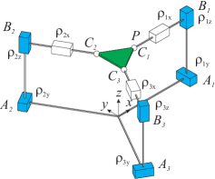
Figure 1: A scheme for the 3-PPPS parallel robot and its parameters in its “home” position with the actuated prismatic joints in blue, the passive joints in white and the mobile platform drawn in green with $x=1/\sqrt{3},y=0,z=0,q_{1}=1,q_{2}=0,q_{3}=0,q_{4}=0$

The coordinates of the point $C_{1}$ are $\rho_{1x}$, $\rho_{1y}$ and $\rho_{1z}$, wherein the last two are actuated. We assume an origin $A_{i}$ for each legs and the equations are given by:

$${\bf A}_{1}=[2,0,0]^{T}$$ (1)

$${\bf A}_{2}=[-1,~{}\sqrt{3},0]^{T}$$ (2)

$${\bf A}_{3}=[-1,-\sqrt{3},0]^{T}$$ (3)

The coordinates of $C_{2}$ and $C_{3}$ are obtained by a rotation around the $z$ axis by $2\pi/3$ and $-2\pi/3$ respectively and the equations are as follows:

$${\bf C}_{1}=[\rho_{1x},\rho_{1y},\rho_{1z}]^{T}$$ (4)

$${\bf C}_{2}=[-\rho_{2x}/2-\sqrt{3}\rho_{2y}/2,\sqrt{3}\rho_{2x}/2-\rho_{2y}/2,\rho_{2z}]^{T}$$ (5)

$${\bf C}_{3}=[-\rho_{3x}/2+\sqrt{3}\rho_{3y}/2,-\sqrt{3}\rho_{3x}/2-\rho_{3y}/2,\rho_{3z}]^{T}$$ (6)

Three locations are now written to describe the mobile platform in the moving frame for an equilateral triangle whose edge lengths are set to one.

$${\bf V}_{1}=[0,0,0]^{T}$$ (7)

$${\bf V}_{2}=[-\sqrt{3}/2,1/2,0]^{T}$$ (8)

$${\bf V}_{3}=[-\sqrt{3}/2,-1/2,0]^{T}$$ (9)

Generally in the robotics community, Euler or Tilt-and-Torsion angles are used to represent the orientation of the mobile platform Caro:2012 . These methods have a physical meaning, but there are singularities to represent certain orientations. The unit quaternions give a redundant representation to define the orientation but at the same time it gives a unique definition for all orientations. The rotation matrix $\bf R$ is described by:

$${\bf R}=\left[\begin{array}[]{ccc}2q_{1}^{2}+2q_{2}^{2}-1&-2q_{1}q_{4}+2q_{2}q_{3}&2q_{1}q_{3}+2q_{2}q_{4}\\ 2q_{1}q_{4}+2q_{2}q_{3}&2q_{1}^{2}+2q_{3}^{2}-1&-2q_{1}q_{2}+2q_{3}q_{4}\\ -2q_{1}q_{3}+2q_{2}q_{4}&2q_{1}q_{2}+2q_{3}q_{4}&2q_{1}^{2}+2q_{4}^{2}-1\end{array}\right]$$ (10)

Here $q_{1}\geq 0$ and $q_{1}^{2}+q_{2}^{2}+q_{3}^{2}+q_{4}^{2}=1$. We can write the coordinates of the mobile platform using the previous rotation matrix as:

$${\bf C}_{i}={\bf R}{\bf V}_{i}+{\bf P}\quad{\rm where}\quad{\bf P}=[x,y,z]^{T}$$ (11)

Thus, we can write the set of constraint equations with the position of $C_{i}$ in the both reference frames by the relations:

$$\rho_{1y}=y$$ (12)

$$\rho_{1z}=z$$ (13)

$$\left(2q_{1}q_{4}-x\right)\sqrt{3}+2{q_{1}}^{2}+3{q_{2}}^{2}-{q_{3}}^{2}-y-2\rho_{2y}=1$$ (14)

$$-\sqrt{3}q_{1}q_{3}+\sqrt{3}q_{2}q_{4}-q_{1}q_{2}-q_{3}q_{4}+\rho_{2z}=z$$ (15)

$$\left(2q_{1}q_{4}+x\right)\sqrt{3}-2{q_{1}}^{2}-3{q_{2}}^{2}+{q_{3}}^{2}-y-2\rho_{3y}=-1$$ (16)

$$-\sqrt{3}q_{1}q_{3}+\sqrt{3}q_{2}q_{4}+q_{1}q_{2}+q_{3}q_{4}+\rho_{3z}=z$$ (17)

0.2.2 Constraint equations

The main problem is to find the location of the mobile platform by looking for the values of the passive prismatic joints $[\rho_{1x},\rho_{1y},\rho_{1z}]$ as proposed in Parenti-Castelli:1990 . The distances between any couple of points $C_{i}$ are given by:

$$||{\bf C}_{1}-{\bf C}_{2}||=||{\bf C}_{1}-{\bf C}_{3}||=||{\bf C}_{2}-{\bf C}_{3}||=1$$ (18)

This method is also used by Chen:2012 for the 3-PPPS by using the dialytic elimination Angeles:2007 . A fourth degree polynomial equation with complicate coefficients is then obtained. However, no self-motion was detected.

Unfortunately, when we want to solve the DKM for the “home” position, i.e. $\rho_{iy}=0$ and $\rho_{iz}=0$ and $i=1,2,3$, we have an infinite number of solutions, which correspond to the self-motion. This result remains the same if we set $\rho_{1z}=\rho_{2z}=\rho_{3z}$. Assuming that this motion is in a plane parallel to the plane (0xy), we write the system coefficients for $\rho_{iz}=0$ with $i=1,2,3$. The fourth degree polynomial then degenerates and a quadratic polynomial equation is obtained which is of the form:

$$9(\rho_{1y}+\rho_{2y}+\rho_{3y})^{2}\rho_{1x}^{2}+$$

$$6\sqrt{3}(\rho_{1y}+\rho_{2y}+\rho_{3y})^{2}(\rho_{2y}-\rho_{3y})\rho_{1x}+$$ (19)

$$(\rho_{1y}+\rho_{2y}+\rho_{3y})^{2}(\rho_{1y}^{2}+2\rho_{1y}\rho_{2y}+2\rho_{1y}\rho_{3y}+4\rho_{2y}^{2}-4\rho_{2y}\rho_{3y}+4\rho_{3y}^{2}-3)=0$$

Here all the terms of the equation cancel out each other when $(\rho_{1y}+\rho_{2y}+\rho_{3y}=0)$. With these conditions, the robot becomes similar to the 3-RPR parallel robot for which its self-motion produces a Cardanic motion. Since the self-motion corresponds to singular configurations, the objective now will be to locate these singularities with respect to other singularities. Geometrically, the self-motion has been described when the motion axes of passive joints intersect at a single point and an angle of $2\pi/3$ is formed between each axis. An example is shown in Fig. 2 where the green mobile platform is one assembly mode obtained in the “home” position. This phenomenon has already been characterized for the 3-RPR parallel robot Chablat:2006 and the PamInsa robot in Briot:2008 .

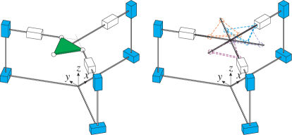
Figure 2: Set of postures to describe the Cardanic motion starting from the “home” position

To validate this result, we use the Siropa library programmed under Maple and its “InfiniteEquations” function Siropa . Three condition are obtained which are $(\rho_{1y}+\rho_{2y}+\rho_{3y}=0)$, $\rho_{1z}=\rho_{2z}$ and $\rho_{2z}=\rho_{3z}$.

0.3 Singularity Analysis

The singular configurations of the 3-PPPS robot have been studied in several articles with either a parametrization of orientations using Euler angles or Quaternions Chablat:2017 . Serial and parallel Jacobian matrices can be computed by differentiating the constraint equations with respect to time Gosselin:1990 ; Sefrioui:92 ; Chablat:1998 . These Jacobian serial and parallel matrices must satisfy the following relationship

$${\bf At+B\dot{\mathbf{\rho}}}=0$$ (20)

where $\bf t$ is the twist of the moving platform and ${\bf\dot{\mathbf{\rho}}}$ is the vector of the active joint velocities.

According to the leg topology of the 3-PPPS robot, there is no serial singularity because the determinant of the ${\bf B}$ matrix does not vanish. Using the same approach as in Caro:2010 , we can determine the matrix ${\bf A}$ and its determinant can be factorized as follows:

$$\left({q_{1}}^{2}-{q_{2}}^{2}-{q_{3}}^{2}+{q_{4}}^{2}\right)\left(q_{1}-q_{4}\right)\left(q_{1}+q_{4}\right)=0$$ (21)

To calculate this result, we use the “ParallelSingularties” function from the Siropa library Siropa . To represent this surface, we eliminate $q_{1}$ thanks to the relation on the quaternions

$$\left({q_{2}}^{2}+{q_{3}}^{2}+2{q_{4}}^{2}-1\right)\left(2{q_{2}}^{2}+2{q_{3}}^{2}-1\right)=0$$ (22)

One of the surface represents a cylinder and the other an ellipsoid. Figure 3 depicts these surfaces bounded by the unit sphere.

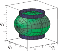
Figure 3: Parallel singularity of the 3-PPPS robot with quaternion representation

By writing the conditions $(\rho_{1y}+\rho_{2y}+\rho_{3y}=0)$ and $\rho_{1z}=\rho_{2z}=\rho_{3z}$ with the constraint equations, the Groebner basis elimination method makes it possible to obtain a set of equations that depends on $q_{2}$, $q_{3}$ and $q_{4}$.

$$q_{2}q_{4}=0$$

$$q_{3}q_{4}=0$$

$$q_{2}\left({q_{2}}^{2}+{q_{3}}^{2}-1\right)=0$$

$$q_{3}\left({q_{2}}^{2}+{q_{3}}^{2}-1\right)=0$$

$${q_{4}}^{3}-q_{4}=0$$

$${q_{2}}^{4}+\left({q_{3}}^{2}+{q_{4}}^{2}-1\right){q_{2}}^{2}+{q_{3}}^{2}{q_{4}}^{2}=0$$ (23)

The intersection of these six equations and the equation 22 is a unit radius circle centered at the origin of the plane $(0q_{2}q_{3})$ as shown in Fig. 4. This circle is tangential to the parallel singularity shown in Fig. 3.

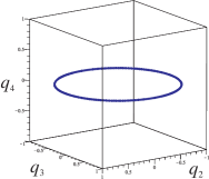
Figure 4: Location of self-motions in the workspace.

As the singularity does not depend on the position, the self-motion exists for an infinite number of positions of the mobile platform. This phenomenon may not be found if numerical methods are used to solve the DKM because the relations $(\rho_{1y}+\rho_{2y}+\rho_{3y}=0)$ and $\rho_{1z}=\rho_{2z}=\rho_{3z}$ are never completely satisfied.

0.4 Conclusions and Perspectives

In this article, we studied the parallel robot 3PPPS to explain the presence of a self-motion at the “home” position. This movement is a Cardanic movement that has already been studied on the 3-RPR parallel robot or the PamInsa robot. Self-motions can often explain the problems of solving the DKM when using algebraic methods. The calculation of a Groebner base makes it possible to detect this problem but the characterization of this movement for robots with six degrees of freedom is difficult because of the size of the equations. Other robots, such as the CaPaMan at the University of Cassino have the same type of singularity despite the phenomenon never being studied. The objective of future work will be to identify architectures with passive prismatic articulations connected to the mobile platform which is capable of having the same singularity conditions.

References

- (1) Husty, M., and Zsombor-Murray, P. (1994), “A special type of singular Stewart-Gough platform,” Advances in Robot Kinematics and Computational Geometry, J. Lenarcic and B. Ravani (eds.), Kluwer Academic Publishers, The Netherlands, pp. 449–458.
- (2) Karger, A. (2002), “Singularities and self motions of a special type of platforms,” Advances in Robot Kinematics, J. Lenarcic and F. Thomas (eds.), Kluwer Academic Publishers, The Netherlands, pp. 449–458.
- (3) Wohlhart, K. (2002), “Synthesis of architecturally mobile double-planar platforms,” Advances in Robot Kinematics, J. Lenarcic and F. Thomas (eds.), Kluwer Academic Publishers, The Netherlands, pp. 473–-482.
- (4) Bonev, I.A., Chablat, D., and Wenger, P. (2006), “Working and assembly modes of the Agile Eye,” Proceedings of the 2006 IEEE International Conference on Robotics and Automation, Orlando, Florida, May 15–19.
- (5) Chablat D., Wenger P. and Bonev I. (2006), “Self Motions of a Special 3-RPR Planar Parallel Robot,” 10th International Symposium on Advances in Robot Kinematics, Kluwer Academic Publishers, Ljubljana, Slovenia, pp. 221–-228, June 25–29.
- (6) Briot S, Bonev I, Chablat D, Wenger P and Arakelian V. (2008), “Self-Motions of General 3-RPR Planar Parallel Robots, International Journal of Robotics Research,” Vol 27(7), pp. 855–866
- (7) Merlet, J. P. (2006), “Parallel robots”, (Vol. 128). Springer Science & Business Media.
- (8) Angeles, J. (2007), “Fundamentals of Robotic Mechanical Systems: Theory, Methods, and Algorithms,” Springer, New York.
- (9) Pierrot, F. and Shibukawa, T. (1998), “From hexa to hexam,” in Internationale Parallel kinematic-Kolloquium (IPK’98), Zurich, pp. 75–84.
- (10) Corbel, D., Company, O., Pierrot, F. (2008), “Optimal Design of a 6-dof Parallel Measurement Mechanism Integrated in a 3-dof Parallel Machine-Tool,” IEEE International Conference on Intelligent Robots and Systems, Nice, pp. 7, September.
- (11) Stoughton, R. and Arai T. A. (1993), “Modified Stewart platform manipulator with improved dexterity,” IEEE Trans. on Robotics and Automation, Vol. 9(2), pp. 166–173, April.
- (12) Ji, Z. and Li, Z. (1999), “Identification of placement parameters for modular platform manipulators,” Journal of Robotic Systems, Vol. 16(4), pp. 227–236.
- (13) Honegger, M., Codourey A., and Burdet, E. (1997), “Adaptive control of the Hexaglide, a 6 dof parallel manipulator,” In IEEE Int. Conf. on Robotics and Automation, pp. 543–548, Albuquerque, April, 21- 28.
- (14) Hunt, K.H. (1983), “Structural kinematics of in parallel actuated robot arms. J. of Mechanisms,” Transmissions and Automation in Design, Vol. 105(4), pp. 705–712, March.
- (15) Chen, C., Gayral, T., Caro, S., Chablat, D., Moroz, G. (2012), “A Six-Dof Epicyclic-Parallel Manipulator,” Journal of Mechanisms and Robotics, American Society of Mechanical Engineers, Vol. 4 (4), pp.041011-1-8.
- (16) Caro, S., Wenger, P. and Chablat, D. (2012), “Non-Singular Assembly Mode Changing Trajectories of a 6-DOF Parallel Robot,” ASME Design Engineering Technical Conferences & Computers and Information in Engineering Conference IDETC/CIE, Chicago, August 12–15, USA.
- (17) Chablat D., Baron L., Jha R. (2017), “Kinematics and workspace analysis of a 3-PPPS parallel robot with U-shaped base,” ASME 2017 International Design Engineering Technical Conferences and Computers and Information in Engineering Conference, Cleveland, Ohio, USA, August 6–9.
- (18) Chablat, D., Baron, L., Jha, R., Rolland, L. (2018), “The 3-PPPS parallel robot with U-shape Base, a 6-DOF parallel robot with simple kinematics”, In 16th International Symposium on Advances in Robot Kinematics, Bologna, July 1-5.
- (19) Caro, S., Moroz, G., Gayral, T., Chablat, D., Chen, C. (2010), “Singularity Analysis of a Six-dof Parallel Manipulator using Grassmann-Cayley Algebra and Gröbner Bases,” Proceedings of an International Symposium on the Occasion of the 25th Anniversary of the McGill University Centre for Intelligent Machines, Nov 2010, Montréal, Canada. pp.341–352.
- (20) Byun, Y.K. and Cho, H-S (1997), “Analysis of a novel 6-dof,3-PPSP parallel manipulator,” Int. J. of Robotics Research, 16(6):859–872, December.
- (21) Parenti-Castelli, V., and Innocenti, C. (1990), “Direct displacement analysis for some classes of spatial parallel mechanisms,” In Proceedings of the 8th CISM-IFTOMM Symposium on Theory and Practice of Robots and Manipulators, pp. 126–130.
- (22) Jha, R., Chablat, D., Barin, L., Rouillier, F. and Moroz, G., Workspace, Joint space and Singularities of a family of Delta-Like Robot Mechanism and Machine Theory, Vol. 127, pp.73–95, September 2018.
- (23) Gosselin, C., Angeles, J. (1990), “Singularity analysis of closed-loop kinematic chains,” IEEE Transactions on Robotics and Automation, 6(3), pp. 281–290.
- (24) Sefrioui, J., Gosselin, C. (1992), “Singularity analysis and representation of planar parallel manipulators,” Robots and autonomous Systems 10, pp. 209–224.
- (25) Chablat D., Wenger Ph., (1998), “Working Modes and Aspects in Fully-Parallel Manipulator,” Proceeding IEEE International Conference on Robotics and Automation, pp. 1964–1969, May.