Fully automated primary particle size analysis of agglomerates on transmission electron microscopy images via artificial neural networks

Abstract

There is a high demand for fully automated methods for the analysis of primary particle size distributions of agglomerates on transmission electron microscopy images. Therefore, a novel method, based on the utilization of artificial neural networks, was proposed, implemented and validated.

The training of the artificial neural networks requires large quantities (up to several hundreds of thousands) of transmission electron microscopy images of agglomerates consisting of primary particles with known sizes. Since the manual evaluation of such large amounts of transmission electron microscopy images is not feasible, a synthesis of lifelike transmission electron microscopy images as training data was implemented.

The proposed method can compete with state-of-the-art automated imaging particle size methods like the Hough transformation, ultimate erosion and watershed transformation and is in some cases even able to outperform these methods. It is however still outperformed by the manual analysis.

1 Introduction

The properties of nanomaterials (e.g. mechanical, optical, catalytic, biological, etc.) are determined by their characteristic length as well as their shape [1]. In case of nanoparticles, the characteristic length is usually some kind of equivalent diameter (e.g. hydrodynamic, volume-based, surface-based, etc.) [2]. There are various techniques available for the determination of the different types of equivalent diameters, one of them being transmission electron microscopy (TEM) [3].

The determination of particle size distributions (PSDs) of non-agglomerated particles on TEM images can already be performed partially or fully automated since several decades [5, 6]. By contrast, the determination of PSDs of agglomerated particles still is a very challenging task for conventional image processing algorithms [7] and therefore still depends on the recognition of primary particles by a human operator. This practice is not only laborious, expensive and repetitive but also error-prone due to the subjectivity and exhaustion of the operator [8].

Therefore, a new approach to imaging particle size analysis, with help of artificial neural networks (ANNs), was proposed, implemented and validated. The ANNs were trained to determine the projected areas of primary particles of agglomerates via regression and the number of primary particles per agglomerate via classification. A major challenge of this approach is the fact that the training of ANNs requires up to several hundreds of thousands of samples with known properties to avoid overfitting, i.e. that the ANN is not able to generate correct outputs for unknown samples because it is too specialized on its training data [9].

Unfortunately, there is no publicly available source of already evaluated samples and a manual evaluation of so many images is hardly feasible, due to the reasons given before. Therefore, inspired by Kruis et al. [10], TEM images with defined characteristics were synthesized and used for the training of the ANNs. To speed up the image synthesis as well as the training of the ANNs the necessary calculations were performed on graphics processing units, whenever possible.

2 State of the Art

Most of the conventional imaging particle size analysis methods are enhancements or combinations of the watershed transformation (WST) [11, 12, 13], ultimate erosion (UE) [14, 15] and/or Hough transformation (HT) [16, 17, 18, 10]. Usually, these methods have one or more parameters, which can be used to control the sensitivity of the primary particle detection. While the availability of such parameters enhances the versatility of the methods, it also impedes their adaptability, because the parameters need to be determined manually prior to the image analysis. Apart from that, none of the methods can compete with the accuracy of a manual evaluation.

So far, to the best of our knowledge, there have only been very few publications concerning the image-based measurement of PSDs with help of ANNs, all of which had a mining context [19, 20]. Therefore, regarding the particle sizes, the image coverage and the utilized image detectors, the specimens that were analyzed in these publications are very different from the specimens that were used in the work at hand. In the context of nanoparticles, several ANN-based methods for the determination of PSDs have been published. However, all of these methods are based on fundamentally different measurement principles (e.g. dynamic light scattering [21, 22], laser diffraction [23, 24] and focused beam reflectance measurement [25, 26]).

3 Artificial Neural Networks

The next sections will address the basic concepts of feed-forward ANNs. The interested reader may refer to literature for a comprehensive treatment of the historical development [27], the fundamentals [28, 29] and the design [30] of ANNs.

An ANN consists of simple computational units called neurons, which are grouped in layers and are unidirectionally connected to each other by weighted connections. In its simplest form an ANN has only one input and one output layer but usually, these are separated by one or more hidden layers (Figure 1). In feed-forward ANNs data may only flow from left to right and there are no loops within the ANN. [29]

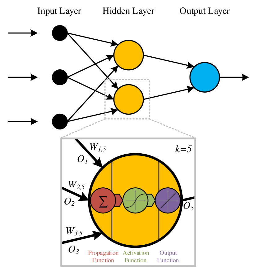
Figure 1: Schematic representation of the common structure of an ANN: input layer, hidden layer and output layer. Magnified: Schematic representation of a neuron.

A neuron typically contains three consecutive functions,which process the data before it is used as input for the following neurons (Figure 1):

1. The propagation function, which transforms the outputs of previous neurons into an input for the current neuron, based on the individual weights of the connections.

2. The activation function, which computes the activation (also referred to as excitement) of the current neuron, based on the input.

3. The output function, which transforms the activation into the output of the current neuron.

3.1 Propagation Function

Usually, a neuron $k$ is connected to multiple preceding neurons $j_{1},j_{2},...,j_{N}$ with the corresponding outputs $\hat{O}=(O_{1},O_{2},...,\allowbreak O_{N})$ via weighted connections with the associated weights $\hat{W}_{k}=(W_{1,k},W_{2,k},...,W_{N,k})$. Since the activation function $f_{act}$ usually expects a scalar input, it is necessary to transfer the vectorial output $\hat{O}$ of the preceding neurons into a scalar input $I_{k}$ for the activation function of the current neuron $k$ by means of a propagation function $f_{prop}$. The most common choice for the propagation function is the weighted sum: [29]

$$I_{k}=f_{prop}(\hat{W}_{k},\hat{O})=\sum_{i=1}^{N}{\left(W_{i,k}\cdot O_{i}\right)}$$

3.2 Activation Function

The activation $A_{k}$ of a neuron $k$ is used as an input for its output function $f_{out}$, to compute its output level $O_{k}$. It depends on the input $I_{k}$ of the neuron, the activation function $f_{act}$ (also called transfer function) and an individual additive bias term $B_{k}$ [28]:

$$A_{k}=f_{act}(I_{k}+B_{k})$$

The most common activation functions are sigmoid functions (e.g. hyperbolic tangent) and the identity function [28]. For the output layers of classification ANNs (see section 3.4) a very common activation function is the softmax function [31].

3.3 Output Function

The output function $f_{out}$ is used to calculate the output $O_{k}$ of a neuron based on its activation [29]:

$$O_{k}=f_{out}(A_{k})$$

Often, the output function is the identity function, so that the output of the neuron equals its activation. Normally, all neurons of an ANN possess the same output function $f_{out}$. [29]

3.4 Learning

In the context of ANNs learning comprises the gradual modification of the properties of an ANN, so that it can correctly predict a certain output for a certain input. The properties of an ANN which are changed during the process of learning are usually the weights of its neurons. Therefore, after the completion of the learning process the weights represent the ”knowledge” of an ANN. [29]

Generally, learning strategies can be grouped into two categories [29]:

• Supervised learning: The ANN is supplied with input data. The error made by the ANN is determined by comparing its output data with the desired correct output data, called target data and used to improve the weights and thereby the performance of the ANN. This process is being repeated until the performance of the ANN is sufficiently good or does not improve within a predefined number of epochs, i.e. repetitions.

• Unsupervised learning: The ANN is only supplied with input data and tries to find similarities and patterns by itself.

In this work, only supervised learning was utilized.

There is a vast variety of different tasks ANNs can learn to solve by means of supervised learning, many of which can be categorized into two groups [32]:

• Classification: When being supplied with a certain input, the ANN outputs a discrete class. An example of a classification could be the assignment of a genre (the output) to a song, based on the year it was published, its length and its dynamics (the inputs).

• Regression: When confronted with a certain input, the ANN outputs a continuous value. An example of a regression could be the determination of the price of a house (the output), based on the year it was built, its location and its number of rooms (the inputs).

For this publication, ANNs were used for classification as well as regression. Firstly, to classify agglomerates with respect to the number of primary particles they incorporate and secondly to regress the individual areas of the primary particles of an agglomerate.

As mentioned before, a supervised learning process is based on the comparison of the actual outputs $\hat{O}=(O_{1},O_{2},...,O_{N})$ of an ANN with the target outputs $\hat{T}=(T_{1},T_{2},...,T_{N})$. To compare the performances of ANNs it is necessary to introduce a criterion for their performance. This criterion is usually implemented in form of a cost (also loss) function. The smaller the cost $C$ of an output, the better the performance of the ANN. Depending on the learning task (regression or classification) of the ANN different cost functions, e.g. mean squared error or cross-entropy (see equation 1 and equation 2 respectively), can be applied. [30]

For regression ANNs the mean squared error is the most common cost function [30, 33]:

$$C_{MSE}(\hat{O},\hat{T})=\frac{1}{N}\sum_{i=1}^{N}(T_{i}-O_{i})^{2}$$ (1)

In contrast, the cross-entropy function is usually used for classification ANNs [30, 33]:

$$C_{CE}(\hat{O},\hat{T})=-\frac{1}{N}\sum_{i=1}^{N}\left(T_{i}\cdot\ln O_{i}\right)$$ (2)

4 Workflow

The workflow of the proposed method consists of a training and a measurement route (Figure 2).

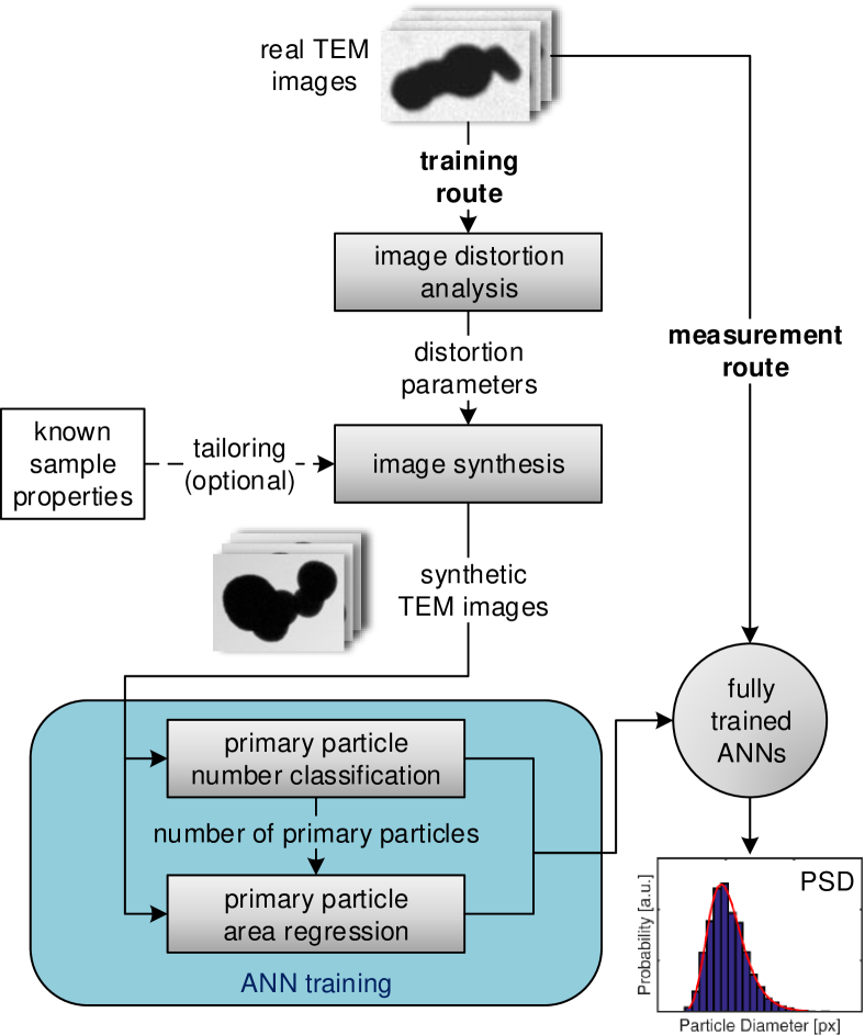
Figure 2: Workflow of the proposed method.

In the first step of the training route, the distributions of the distortion parameters of real TEM images are determined, to use them during the image synthesis to obtain more lifelike synthetic TEM images. Three characteristic image distortions are considered and quantified with suitable measurands (Table 1).

Table 1: Measurands of characteristic image distortions.

Distortion	Measurands
blur	Tenenbaum’s gradient focus measure [34]
noise	standard deviation of the pixel intensities
nonuniform illumination	1-1-polynomial fit of the pixel intensities

The image synthesis is a central element of the proposed method because it represents a feasible way to obtain the large number of images with known target properties, which is necessary for the training of the ANNs. It is of utmost importance to synthesize images which are as lifelike as possible, to provide realistic training data for the ANNs. Elsewise, the ANNs might perform well on the training data but will fail once they are applied to real TEM images. Additionally, the image synthesis provides an opportunity for the incorporation of a priori knowledge about the product, which is going to be analyzed. Thus, the training data of the ANNs can be tailored to the product properties, to facilitate the training and improve the measurement quality.

To reduce the amount of input data and thereby the computational effort during the training and utilization of the ANNs, the input images are preprocessed. As preprocessing, 13 features (Table 5) of each agglomerate are determined and used as input of the ANNs.

There are two different types of ANNs, which are used during the determination of primary PSDs via the proposed method. On the one hand, there is a classification ANN, which determines the number of primary particles an agglomerate incorporates. On the other hand, there are multiple regression ANNs, which are utilized for the regression of the primary particle areas of an agglomerate, depending on the number of primary particles it incorporates. This means that for each class of agglomerates an individual regression ANN is used. The reason for this two-step strategy is the fact that the number of outputs of an ANN needs to be defined a priori and cannot be determined by the ANN itself during its run-time. It is important to note that this limits the maximum number of primary particles an agglomerate may contain while still being analyzed, to the number of regression ANNs which are trained beforehand. Agglomerates containing a higher number of primary particles are simply sorted out by the classification ANN and thereby excluded from the analysis. For this publication, five regression ANNs were trained, i.e. the number of primary particles per agglomerate was limited to five.

After the training of the ANNs has been finished, they can be used for the determination of primary PSDs via the measurement route.

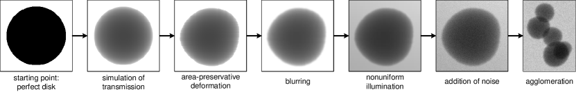
Figure 3: Elementary steps of the image synthesis.

5 Image Synthesis

Starting with a perfectly circular black disk, the image synthesis basically consists of six steps (see also figure 3):

1. Simulation of electron transmission
   For an amorphous spherical object with an outer radius $R$, the transmission ratio at a radius ${0\leq r\leq R}$ is given by:

   $$\frac{I_{T}}{I_{0}}=\exp{(-2c_{T}\cdot\sqrt{R^{2}-r^{2}})}$$

   $I_{0}$ and $I_{T}$ are the intensities before and after the transmission and $c_{T}$ is the transmission coefficient, which depends on the density, the atomic weight and number of the material, as well as the aperture angle and the acceleration voltage of the instrument. [35]

2. Area-preservative deformation
   Until now the synthesized particles are perfectly spherical and their two-dimensional projections are therefore perfectly circular. Since this does not apply to most naturally occurring particles, it is necessary to deform the circular form. The challenge of the deformation process is the preservation of the projection area, as it is the measurand of the proposed method.

3. Blurring
   The blur synthesis is based on the distribution of the standard deviation of the Gaussian blur, which was determined based on Tenenbaum’s gradient focus measure [34], during the image distortion analysis of real TEM images.

4. Nonuniform illumination
   For the synthesis of the nonuniform illumination, the distributions of the parameters of the 1-1-polynomial, which were determined during the image distortion analysis of real TEM images, are utilized.

5. Addition of noise
   As noise for the synthetic TEM image, a Gaussian noise with a standard deviation according to the distribution, which was determined during the image distortion analysis of real TEM images, is used.

6. Agglomeration
   So far, the image synthesis has been limited to single particles. However, since the ANNs need to be trained on images of agglomerates, an agglomeration algorithm was implemented. Due to the large number of images, which are necessary for the training of the ANNs, one of the most important requirements concerning the agglomeration algorithm is a high computation speed. Therefore, complex agglomeration simulations (e.g. kinetic particle simulations) were not an option. Instead, the agglomerates are constructed geometrically, by joining spheres at random surface points, while avoiding overlaps of the spheres.

Ultimately, the image synthesis yields synthetic TEM images, which are lifelike to a large extent (see supplementary material).

6 Primary Particle Number Classification

The following section will elaborate upon the design, training, validation and results of the ANN, which was used for the classification of agglomerates according to their number of primary particles (hereinafter called ParticleNumberNet). Since each class of agglomerates requires its own ANN for the regression of its primary particle areas (hereinafter called ParticleAreaNets), it was necessary to limit the number of classes, i.e. the maximum number of primary particles per agglomerate, to reduce the design effort, as well as the computation times during the training and utilization of the ANN. It was therefore decided to limit the classification to six classes: one for each number of primary particles from one to five and one for agglomerates containing more than five primary particles, which are not being analyzed.

6.1 Training, Validation and Test Data

The input data set which was used for the training of the ParticleNumberNet was generated by synthesizing 100,000 images of each class of agglomerates, where the class of agglomerates which consist of more than five primary particles contained agglomerates with up to 10 primary particles. The area of the primary particles was homogeneously distributed across all synthesized images and varied in the range of approximately $5006500\text{\,}\mathrm{pixels}$. The homogeneous distribution of the primary particle area was important to prevent the ANN from developing preferences concerning the recognition of particles with areas overrepresented in the input data.

Subsequently, the images were segmented, i.e. the foreground was separated from the background, and the agglomerates were characterized by 13 features (Table 5). To prevent features with large ranges (e.g. area) from overriding features with small ranges (e.g. mean intensity), the features were normalized based on their individual ranges.

The target data for the training of the ParticleNumberNet consisted of a total of 600,000 binary vectors with six components each, where each of the six components represented the probability to belong to one of the six classes, i.e. either 0 or 1. The input and target data was divided into three subsets (Table 8), to evaluate the generalization abilities of the ANN and to allow the utilization of the early stopping method [32].

6.2 Structural Optimization

The final structure of the ParticleNumberNet and the learning strategies utilized during its training are given in tables 6 and 7 respectively.

To yield optimal results, the structure of the ParticleNumberNet was optimized iteratively. Some structural features of ANNs depend solely on the structure of the input and the target data. Every ANN has exactly one input layer, whose number of neurons $N_{i}$ is equal to the number of components of an input sample (in case of the ParticleNumberNet $N_{i}=13$). Additionally, every ANN has exactly one output layer, whose number of neurons is equal to the number of components of a target sample (in case of the ParticleNumberNet $N_{o}=6$). In contrast, the number of hidden layers and the numbers of neurons $N_{h,i}$ in those layers can be modified freely. However, it is uncommon for feed-forward ANNs to have more than two hidden layers [30], because two hidden layers already allow the ANN to approximate all possible kinds of functions [36]. Therefore, only ANN structures with up to two hidden layers were tested as candidates for the ParticleNumberNet and the ParticleAreaNets.

More important than the number of hidden layers is the number of neurons within these layers. Unfortunately, there are no strict rules for the dimensioning of hidden layers. [36]

However, there are rules of thumb which can be used as an orientation [36]:

$\displaystyle N_{o}$ $\displaystyle\leq N_{h,i}<2N_{i}$ (3) $\displaystyle\Rightarrow$ $\displaystyle 6$ $\displaystyle\leq N_{h,i}<26$

$\displaystyle N_{h,i}$ $\displaystyle\approx\nicefrac{{2}}{{3}}N_{i}+N_{o}$ (4) $\displaystyle\Rightarrow$ $\displaystyle N_{h,i}$ $\displaystyle\approx 15$

To find the optimum for the number of neurons of the two hidden layers, all possible combinations of ${1\leq N_{h,1}<26}$ and ${0\leq N_{h,2}<26}$ were assessed. Due to the high number of ANNs which needed to be tested, it was not feasible to use all available data but only a subset of it. To find the sufficient number of samples, an ANN with two hidden layers of 25 neurons each was tested with varying amounts of input data. The reason for the choice of ${N_{h,1}=N_{h,2}=25}$ is the fact that the required number of samples increases with the number of degrees of freedom of an ANN, which in turn increases with the number of layers as well as with the number of neurons. Therefore, it was reasonable to determine the number of required samples on the largest ANN which was going to be tested. As a measure of quality, the minimum cost, i.e. the cross-entropy, achieved by the ANN on the test set during 200 epochs of training was used. Due to the influence of the random initialization of the ANN, each measurement was repeated for ten different random seeds and the mean of the results was calculated.

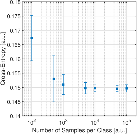
Figure 4: Cross-entropy as a function of the number of samples per class for a ParticleNumberNet with two hidden layers of 25 neurons each. Please note the logarithmic scale of the $x$-axis.

Figure 4 displays the results of the investigation of the influence of the number of samples on the quality of the ANN. The mean and the standard deviation of the cross-entropy decrease with an increasing number of samples but do not improve further in the region above 10,000 samples per class. Therefore, a number of 10,000 samples per class was identified as being sufficient for the investigation of the optimal structure of the ParticleNumberNet.

For the investigation of the optimal structure of the ParticleNumberNet, 10,000 samples per class were shuffled and randomly split into three sets (Table 8). Subsequently, the lowest cross-entropy achieved by the ANN on the test set during 200 epochs of training was determined for each combination of ${1\leq N_{h,1}<26}$ and ${0\leq N_{h,2}<26}$. Due to the influence of the random initialization of the ANNs, each measurement was repeated for ten different random seeds and the mean of the results was calculated. Ultimately, the investigation yielded that no significant improvements could be achieved by the incorporation of a second hidden layer. However, better results were achieved for higher numbers of neurons in the first hidden layer. Therefore, the assessment described above was repeated for ParticleNumberNets with a single hidden layer of up to 100 neurons. The resulting means of the minimum cross-entropies were normalized via a division by the mean of the minimum cross-entropies of the ANNs with a single hidden neuron and plotted versus the number of hidden neurons.

The resulting graph (Figure 5) was fitted by a function of the form

$$f(x)=\frac{ax^{3}+bx^{2}+cx+d}{x+e},$$

which was empirically found to fit the results best and exhibits a minimum for 39 neurons in the hidden layer. It was therefore decided to incorporate 39 hidden neurons in the final structure of the ParticleNumberNet (Table 6).

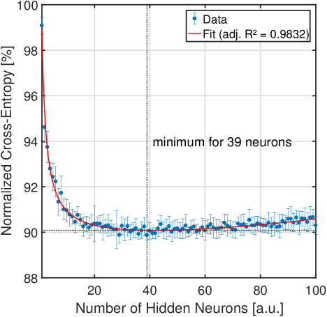
Figure 5: Cross-entropy, normalized based on the maximum cross-entropy which was encountered, for different numbers of neurons in the hidden layer of the ParticleNumberNet.

6.3 Validation and Results

To validate the proposed method with regard to the classification of the number of primary particles incorporated by an agglomerate, its performance was compared to those of three established automated methods (WST, UE and HT) as well as those of the manual method, once for synthesized and once for real TEM images. To account for the human factor, the manual method was performed independently by two different test persons.

The three established automated methods were implemented according to the MATLAB documentation [33] and their parameters were empirically optimized, to prevent a discrimination of the established automated methods compared to the proposed method.

6.3.1 Synthetic Data

The set of synthetic TEM images for the assessment of the classification performance consisted of 15,000 synthetic TEM images for each class of agglomerates, i.e. 90,000 images in total. All samples had different PSDs, different transmission coefficients and different degrees of particle deformation. The distortion parameters of the synthesized TEM images were chosen randomly according to their distributions, which were determined beforehand based on real TEM images.

Due to its extremely labor-intensive nature, the manual method was performed on a reduced set of just 100 images per class, i.e. 600 images in total.

The results of the validation based on synthetic TEM images can be found in table 2. The proposed method can outperform the established automated methods but is still inferior to the manual evaluation.

Table 2: Ranking of the mean classification accuracies of the proposed method and established automated methods on a data set of 90,000 synthetic transmission electron microscopy images, as well as of the manual method on a data set of 600 synthetic transmission electron microscopy images.

	Mean Classification Accuracy
Test Person A	$88.3\text{\,}\mathrm{\char 37\relax}$
Test Person B	$84.0\text{\,}\mathrm{\char 37\relax}$
Proposed Method	$63.8\text{\,}\mathrm{\char 37\relax}$
Hough Transformation	$55.0\text{\,}\mathrm{\char 37\relax}$
Ultimate Erosion	$48.2\text{\,}\mathrm{\char 37\relax}$
Watershed Transformation	$46.5\text{\,}\mathrm{\char 37\relax}$

6.3.2 Real Data

The set of real TEM images for the assessments of the classification performance consisted of 500 real TEM images of agglomerates. Due to the reason that the actual number of primary particles depicted on a real TEM image cannot be determined definitively, the results of the manual measurements of test person A, who performed best on the synthetic TEM images (Table 2), were used as ground truth.

In contrast to the set of synthetic TEM images, which was used for the assessment of the classification performance, the set of real TEM images did not contain an equal number of samples of each class (Table 9), due to the limited availability of suitable TEM images. This circumstance should be considered, when trying to compare the results of the assessment of the classification performance based on synthetic TEM images to those of the assessment based on real TEM images.

The results of the validation based on real TEM images can be found in table 3. Just like in the case of synthetic TEM images, the proposed method can outperform the three established automated methods but still lacks the accuracy of the manual method.

Table 3: Ranking of the mean classification accuracies of the proposed method, established automated methods and the manual evaluation on a data set of 500 real transmission electron microscopy images (ground truth: manual evaluation of test person A).

	Mean classification accuracy
Test Person B	$68.2\text{\,}\mathrm{\char 37\relax}$
Proposed Method	$60.8\text{\,}\mathrm{\char 37\relax}$
Ultimate Erosion	$59.0\text{\,}\mathrm{\char 37\relax}$
Watershed Transformation	$53.8\text{\,}\mathrm{\char 37\relax}$
Hough Transformation	$23.2\text{\,}\mathrm{\char 37\relax}$

7 Primary Particle Area Regression

The following section will elaborate upon the design, training, validation and results of the ANNs, which were used for the regression of the areas of the primary particles of an agglomerate (hereinafter called ParticleAreaNets). As mentioned above, each class of agglomerates, except the mixed sixth class which contained agglomerates with more than five primary particles and was therefore excluded from the analysis, needed to be analyzed by an individual ParticleAreaNet.

7.1 Training, Validation and Test Data

The input data used for the training of the ParticleAreaNets was identical to the training data of the ParticleNumberNet but was divided into individual data sets for each class of agglomerates.

The target data sets for the training of the ParticleAreaNets consisted of 100,000 vectors per class, where each of the vectors had a number of components equal to the number of primary particles in an agglomerate of the corresponding class. The components contained the areas of the primary particles.

Just like before, each input and target data set was divided into three subsets (Table 12), to evaluate the generalization abilities of the ANNs and to allow the utilization of the early stopping method.

7.2 Structural Optimization

The final structures of the ParticleAreaNets and the learning strategies utilized during their training are given in tables 10 and 11 and in table 13 respectively.

To yield optimal results, the structures of the ParticleAreaNets were again optimized iteratively. The number of neurons in the input and output layers of the ParticleAreaNets are defined by the number of components of input ($N_{i}=13$) and output samples ($1\leq N_{o}\leq 5$) respectively. Due to the reasons given before, only ANN structures with up to two hidden layers were tested as ParticleAreaNets.

In case of the ParticleAreaNets the rules of thumb (see equations 3 and 4) [36], yield the following numbers of neurons as orientation for the optimization of the hidden layers:

$\displaystyle 1..5$ $\displaystyle\leq N_{h,i}<26$

$\displaystyle N_{h,i}$ $\displaystyle\approx 10..14$

Before the assessment of the optimal number of neurons in the hidden layers of the ParticleAreaNets, the necessary number of input samples was determined. The ParticleAreaNet with the most degrees of freedom, i.e. with the highest number of neurons was used for the evaluation. The ParticleAreaNet with the highest number of neurons is the ParticleAreaNet for agglomerates with five primary particles ($N_{o}=5$) and two hidden layers of 25 neurons each (${N_{h,1}=N_{h,2}=25}$). As a measure of quality of the ANN, the minimum cost, i.e. the mean squared error, achieved by the ANN on the test set during 200 epochs of training was used. Due to the influence of the random initialization of the ANN, each measurement was repeated for ten different random seeds and the mean of the results was calculated.

Figure 6 displays the results of the investigation of the influence of the number of samples on the quality of the ANN. The mean and the standard deviation of the mean squared error decrease with an increasing number of samples, but do not further improve in the region above 10,000 samples per class. Therefore, a number of 10,000 samples per class was identified as being sufficient for the investigation of the optimal structures of the ParticleAreaNets.

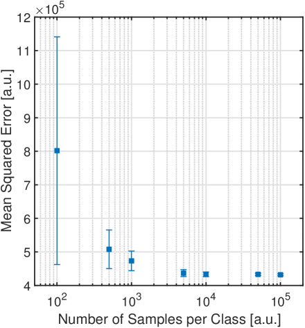
Figure 6: Mean squared error as a function of the number of samples per class for a ParticleAreaNet for agglomerates containing five primary particles with two hidden layers of 25 neurons each. Please note the logarithmic scale of the $x$-axis.

For the assessment of the optimal numbers of neurons in the hidden layers of the ParticleAreaNets, all possible combinations of ${1\leq N_{h,1}<26}$ and ${0\leq N_{h,2}<26}$ were tested for each of the ParticleAreaNets. The assessment was performed similarly to the procedure described in section 6.2. For each of the ParticleAreaNets, 10,000 samples were shuffled and randomly split into three sets (Table 12). Subsequently, the lowest mean squared errors achieved by the ParticleAreaNets on the respective test sets during 200 epochs of training were determined for each combination of ${1\leq N_{h,1}<26}$ and ${0\leq N_{h,2}<26}$. Due to the influence of the random initialization of the ANNs, each measurement was repeated for ten different random seeds and the means of the results were calculated for the different ParticleAreaNets. Ultimately, the investigation yielded that no significant improvements could be achieved by the incorporation of a second hidden layer. However, better results were achieved for higher numbers of neurons in the first hidden layer. Therefore, the assessment described above was repeated for ParticleAreaNets with single hidden layers of up to 400 neurons. The resulting means of the minimum mean squared errors were normalized via a division by the mean of the minimum mean squared errors of the ANNs with a single hidden neuron and plotted versus the number of hidden neurons. The resulting graphs (e.g. figure 7; for further information please refer to the supplementary material) were fitted by functions of the form

$$f(x)=\frac{ax^{3}+bx^{2}+cx+d}{x+e},$$

which were empirically found to fit the results best. The numbers of neurons in the hidden layers of the final structures of the ParticleAreaNets (Tables 10 and 11) were set to the number of neurons where the respective fits exhibited their minima.

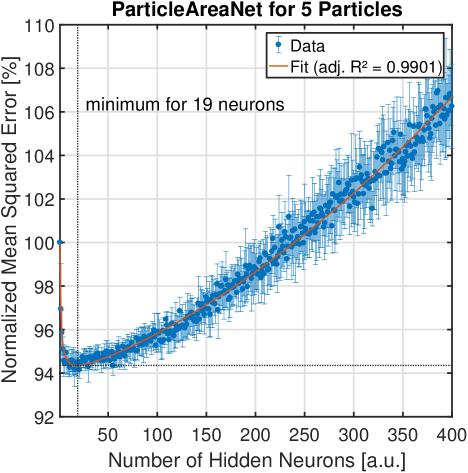
Figure 7: Mean squared error, normalized based on the maximum mean squared error which was encountered, for different numbers of neurons in the hidden layer of the ParticleAreaNet for agglomerates containing five primary particles.

7.3 Validation and Results

To validate the proposed method with regard to the measurement of PSDs, its performance was compared to those of the three established automated methods as well as those of the manual method, once for synthesized and once for real TEM images. To account for the human factor, the manual method was performed independently by two different test persons.

7.3.1 Synthetic Data

The set of samples of synthetic TEM images for the assessments of the performance of the PSD measurement consisted of 300 samples with 500 agglomerates each. The number of agglomerates was chosen so that the minimum number of particles of a sample was 500 (for a sample containing only single particles), which is considered to be the necessary minimum for a good statistical quality of PSD measurements [38]. All samples had different geometric mean diameters (GMDs) and geometric standard deviations (GSDs), different distributions of primary particles per agglomerate, different transmission coefficients and different degrees of particle deformation. The distortion parameters of the synthesized TEM images were chosen randomly according to their distributions, which were determined beforehand based on real TEM images.

Due to its extremely labor-intensive nature, the manual method was performed on a reduced set of just one sample of 500 agglomerates.

For the assessment of the PSD measurement performance, the output GMD $d_{g,O}$ and output GSD $\sigma_{g,O}$ of each sample were determined based on the output primary particle areas, which were measured via the different methods and compared to the corresponding target GMD $d_{g,T}$ and target GSD $\sigma_{g,T}$, which were determined based on the known target primary particle areas. Subsequently, the relative errors $E_{d_{g}}$ and $E_{\sigma_{g}}$ of the GMD and GSD were calculated:

$\displaystyle E_{d_{g}}$ $\displaystyle=\frac{d_{g,O}-d_{g,T}}{d_{g,T}}$ (5)

$\displaystyle E_{\sigma_{g}}$ $\displaystyle=\frac{\sigma_{g,O}-\sigma_{g,T}}{\sigma_{g,T}}$ (6)

Ultimately, the relative errors of the GMD and GSD were plotted in form of histograms for each of the methods.

Figure 8 exemplarily depicts the histograms of the relative errors of the GMD and GSD of the primary PSDs of 300 samples of 500 synthetic TEM images each, which were determined via the proposed method. It can be noticed that the proposed method tends to overestimate the GMD as well as the GSD of primary PSDs. For the results of the other methods, which were tested, please refer to the supplementary material.

Proposed Method

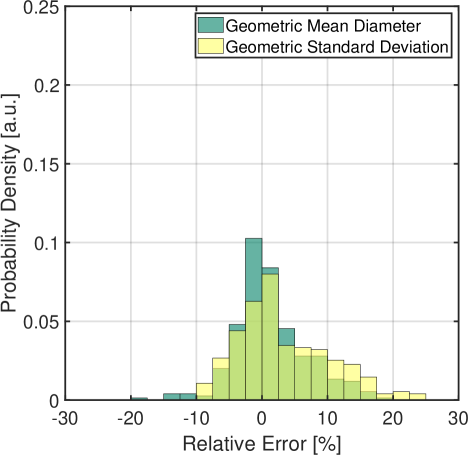
Figure 8: Histograms of the errors of geometric mean diameter and geometric standard deviation determined by the proposed method when being applied to synthetic transmission electron microscopy images.

7.3.2 Real Data

The set of real TEM images for the assessments of the performance of the PSD measurement consisted of 500 real TEM images in total. Due to the reason that the actual areas of the primary particles depicted on a real TEM image cannot be determined definitively, the results of the manual measurements of test person A, who performed best on the synthetic data, were used as ground truth to calculate the relative errors of the GMD and the GSD according to equation 5 and 6 respectively.

It is hardly possible to evaluate the performances of the tested methods concerning the measurement of PSDs of real samples based on just one sample. It can, however, help to get a basic idea of the potential of the methods.

The deviations of the GMD and the GSD, which were determined during the validation can be found in table 4. The proposed method clearly outperforms the three established methods with respect to the determination of the GMD. In case of the determination of the GSD, only the UE can outperform the proposed method. In general, all automated methods lack the accuracy of the manual method.

Table 4: Relative errors of the geometric mean diameter and the geometric standard deviation determined via the proposed method, established automated methods and the manual evaluation on a data set of 500 real transmission electron microscopy images (ground truth: manual evaluation of test person A).

	Relative Error of the GMD	Relative Error of the GSD
Proposed Method	$4.1\text{\,}\mathrm{\char 37\relax}$	$5.1\text{\,}\mathrm{\char 37\relax}$
Watershed Transformation	$-11.6\text{\,}\mathrm{\char 37\relax}$	$6.1\text{\,}\mathrm{\char 37\relax}$
Ultimate Erosion	$-10.7\text{\,}\mathrm{\char 37\relax}$	$1.5\text{\,}\mathrm{\char 37\relax}$
Hough Transformation	$-20.1\text{\,}\mathrm{\char 37\relax}$	$8.7\text{\,}\mathrm{\char 37\relax}$
Test Person B	$-4.3\text{\,}\mathrm{\char 37\relax}$	$-1.0\text{\,}\mathrm{\char 37\relax}$

8 Conclusion

Within this work, a novel method for the analysis of the size of primary particles of agglomerates on TEM images was successfully implemented and validated. Therefore, a two-stage strategy was applied: During the first stage, each agglomerate is assigned to a class, depending on the number of primary particles it incorporates, by a classification ANN. Subsequently, the areas of the incorporated primary particles are analyzed by a regression ANN that is specific to the class of the agglomerate.

Regarding the classification performance, the proposed method is superior to the WST, HT and UE. However, for reasons of fairness, it should be noted that none of the established automated methods was designed specifically for the determination of the number of primary particles in agglomerates. Another result of the evaluation of the classification performance is that the proposed method, as well as the established automated methods, are clearly outperformed by the manual method.

With respect to the determination of primary PSDs of agglomerates on TEM images, the evaluation of the performance is especially difficult because only a single real sample of TEM images was available. However, for this sample, as well as for samples of synthetic TEM images, the validation yielded very promising results for the proposed method. Again, the manual method could outperform all other tested methods.

All in all, the proposed method is not able to match the accuracy of the manual evaluation. Nevertheless, it is at least able to compete with established automated methods, which have been used and improved for several decades. It may be assumed that its performance could be further improved and may therefore be able to outperform the established automated methods more clearly and perhaps even reach the accuracy of the manual method while offering significantly shorter measurement times.

Appendix A Preprocessing

Table 5: Agglomerate features determined during the preprocessing process.

Area	Number of pixels within the agglomerate.
Convex area	Number of pixels within the convex hull of the agglomerate.
Eccentricity	Eccentricity of an ellipse with second moments equal to those of the agglomerate.
Equivalent diameter	Diameter of a circle with an area equal to the area of the agglomerate.
Extent	Ratio of the areas of the agglomerate and its bounding box.
Filled area	Number of pixels within the agglomerate, after all potential holes have been filled.
Major axis length	Length of the major axis of an ellipse with normalized second central moments equal to those of the agglomerate.
Minor axis length	Length of the minor axis of an ellipse with normalized second central moments equal to those of the agglomerate.
Perimeter	Number of pixels surrounding the agglomerate.
Solidity	Ratio of area and convex area of the agglomerate.
Minimum intensity	Intensity of the darkest pixel in the region.
Maximum intensity	Brightest pixel in the region.
Mean intensity	Mean of the intensities of the pixels of the region.

Appendix B Primary Particle Number Classification

Table 6: Structural features of the artificial neural network for the classification of agglomerates with respect to the number of primary particles.

	Input layer	Hidden layer	Output layer
Propagation function	identity	weighted sum	weighted sum
Activation function	identity	hyperbolic tangent	softmax
Output function	identity	identity	identity
Number of neurons	13	39	6

Table 7: Learning features of the artificial neural network for the classification of agglomerates with respect to the number of primary particles.

Cost function	cross-entropy
Learning rule	scaled conjugate gradient backpropagation [39]
Overfitting prevention	early stopping
Number of samples per class	100,000
Number of epochs	100,000

Table 8: Division of the data used to train and evaluate the artificial neural network for the classification of agglomerates with respect to the number of primary particles.

Training set:	$70\text{\,}\mathrm{\char 37\relax}$
Validation set:	$15\text{\,}\mathrm{\char 37\relax}$
Test set:	$15\text{\,}\mathrm{\char 37\relax}$

Table 9: Composition of the set of real transmission electron microscopy images for the assessment of the primary particle number classification performance as classified by test person A.

	Number of samples
1 particle	234
2 particles	153
3 particles	64
4 particles	26
5 particles	9
5+ particles	14

Appendix C Primary Particle Area Regression

Table 10: Structural features of the artificial neural networks for the regression of primary particle areas.

	Input layer	Hidden layer	Output layer
Propagation function	identity	weighted sum	weighted sum
Activation function	identity	hyperbolic tangent	identity
Output function	identity	identity	identity

Table 11: Numbers of neurons in the layers of the artificial neural networks for the regression of primary particle areas.

	Number of neurons
Number of primary particles	Input layer	Hidden layer	Output layer
1	13	11	1
2	13	124	2
3	13	104	3
4	13	29	4
5	13	19	5

Table 12: Division of the data used to train and evaluate the artificial neural networks for the regression of primary particle areas.

Training set:	$70\text{\,}\mathrm{\char 37\relax}$
Validation set:	$15\text{\,}\mathrm{\char 37\relax}$
Test set:	$15\text{\,}\mathrm{\char 37\relax}$

Table 13: Learning features of the artificial neural networks for the regression of primary particle areas.

Cost function	mean squared error
Learning rule	scaled conjugate gradient backpropagation [39]
Overfitting prevention	early stopping
Number of samples	100,000
Number of epochs	100,000

References

- [1] G. Guisbiers, S. Mejía-Rosales, F. Leonard Deepak, Nanomaterial properties: Size and shape dependencies, Journal of Nanomaterials 2012 (2012) 1–2. doi:10.1155/2012/180976.
- [2] J. G. Calvert, Glossary of atmospheric chemistry terms (recommendations 1990), Pure and Applied Chemistry 62 (11). doi:10.1351/pac199062112167.
- [3] E. J. Cho, H. Holback, K. C. Liu, S. A. Abouelmagd, J. Park, Y. Yeo, Nanoparticle characterization: state of the art, challenges, and emerging technologies, Molecular pharmaceutics 10 (6) (2013) 2093–2110. doi:10.1021/mp300697h.
- [4] EK, Commission recommendation of 18 october 2011 on the definition of nanomaterial (2011/696/eu), Official journal of the European Union.
- [5] R. P. King, Determination of the distribution of size of irregularly shaped particles from measurements on sections or projected areas, Powder Technology 32 (1) (1982) 87–100. doi:10.1016/0032-5910(82)85009-2.
- [6] R. P. King, Measurement of particle size distribution by image analyser, Powder Technology 39 (2) (1984) 279–289. doi:10.1016/0032-5910(84)85045-7.
- [7] P.-J. de Temmerman, E. Verleysen, J. Lammertyn, J. Mast, Semi-automatic size measurement of primary particles in aggregated nanomaterials by transmission electron microscopy, Powder Technology 261 (2014) 191–200. doi:10.1016/j.powtec.2014.04.040.
- [8] T. Allen, Powder sampling and particle size determination, 1st Edition, Elsevier, Amsterdam and Boston, 2003.
- [9] M. A. Babyak, What you see may not be what you get: a brief, nontechnical introduction to overfitting in regression-type models, Psychosomatic medicine 66 (3) (2004) 411–421.
- [10] F. E. Kruis, J. van Denderen, H. Buurman, B. Scarlett, Characterization of agglomerated and aggregated aerosol particles using image analysis, Particle & Particle Systems Characterization 11 (6) (1994) 426–435. doi:10.1002/ppsc.19940110605.
- [11] C. Jung, C. Kim, Segmenting clustered nuclei using h-minima transform-based marker extraction and contour parameterization, IEEE transactions on bio-medical engineering 57 (10 PART 2) (2010) 2600–2604. doi:10.1109/TBME.2010.2060336.
- [12] J. Shu, H. Fu, G. Qiu, P. Kaye, M. Ilyas, Segmenting overlapping cell nuclei in digital histopathology images, in: 2013 35th annual international conference of the IEEE Engineering in Medicine and Biology Society (EMBC), IEEE, Piscataway, NJ, 2013, pp. 5445–5448. doi:10.1109/EMBC.2013.6610781.
- [13] J. Cheng, J. C. Rajapakse, Segmentation of clustered nuclei with shape markers and marking function, IEEE transactions on bio-medical engineering 56 (3) (2009) 741–748. doi:10.1109/TBME.2008.2008635.
- [14] Z. Wang, A semi-automatic method for robust and efficient identification of neighboring muscle cells, Pattern Recognition 53 (2016) 300–312. doi:10.1016/j.patcog.2015.12.009.
- [15] C. Park, J. Z. Huang, J. X. Ji, Y. Ding, Segmentation, inference and classification of partially overlapping nanoparticles, IEEE transactions on pattern analysis and machine intelligence 35 (3) (2013) 669–681. doi:10.1109/TPAMI.2012.163.
- [16] D. Ballard, Generalizing the hough transform to detect arbitrary shapes, Pattern Recognition 13 (2) (1981) 111–122. doi:10.1016/0031-3203(81)90009-1.
- [17] P. M. Merlin, D. J. Farber, A parallel mechanism for detecting curves in pictures, IEEE Transactions on Computers C-24 (1) (1975) 96–98. doi:10.1109/T-C.1975.224087.
- [18] L. Xu, E. Oja, P. Kultanen, A new curve detection method: Randomized hough transform (rht), Pattern Recognition Letters 11 (5) (1990) 331–338. doi:10.1016/0167-8655(90)90042-Z.
- [19] Y.-D. Ko, H. Shang, A neural network-based soft sensor for particle size distribution using image analysis, Powder Technology 212 (2) (2011) 359–366. doi:10.1016/j.powtec.2011.06.013.
- [20] E. Hamzeloo, M. Massinaei, N. Mehrshad, Estimation of particle size distribution on an industrial conveyor belt using image analysis and neural networks, Powder Technology 261 (2014) 185–190. doi:10.1016/j.powtec.2014.04.038.
- [21] G. Stegmayer, O. Chiotti, L. Gugliotta, J. Vega, Particle size distribution from combined light scattering measurements. a neural network approach for solving the inverse problem, in: Proceedings of 2006 IEEE International Conference on Computational Intelligence for Measurement Systems and Applications, IEEE Service Center, Piscataway, NJ, 2006, pp. 91–95. doi:10.1109/CIMSA.2006.250762.
- [22] L. M. Gugliotta, G. S. Stegmayer, L. A. Clementi, V. D. G. Gonzalez, R. J. Minari, J. R. Leiza, J. R. Vega, A neural network model for estimating the particle size distribution of dilute latex from multiangle dynamic light scattering measurements, Particle & Particle Systems Characterization 26 (1-2) (2009) 41–52. doi:10.1002/ppsc.200800010.
- [23] R. Guardani, C. Nascimento, R. Onimaru, Use of neural networks in the analysis of particle size distribution by laser diffraction: Tests with different particle systems, Powder Technology 126 (1) (2002) 42–50. doi:10.1016/S0032-5910(02)00036-0.
- [24] C. Nascimento, R. Guardani, M. Giulietti, Use of neural networks in the analysis of particle size distributions by laser diffraction, Powder Technology 90 (1) (1997) 89–94. doi:10.1016/S0032-5910(96)03192-0.
- [25] C. F. Maússe, Use of artificial neural network models to derive particle size distributions and their moments from chord length distributions, Ph.D. thesis (2006).
- [26] R. Irizarry, A. Chen, R. Crawford, L. Codan, J. Schoell, Data-driven model and model paradigm to predict 1d and 2d particle size distribution from measured chord-length distribution, Chemical Engineering Science 164 (2017) 202–218. doi:10.1016/j.ces.2017.01.042.
- [27] J. Schmidhuber, Deep learning in neural networks: an overview, Neural networks : the official journal of the International Neural Network Society 61 (2015) 85–117. doi:10.1016/j.neunet.2014.09.003.
- [28] S. S. Haykin, Neural networks and learning machines, 3rd Edition, Pearson Prentice-Hall, New York, 2009.
-
[29]
D. Kriesel, A brief introduction to neural
networks (2007).
URL http://www.dkriesel.com - [30] M. T. Hagan, H. B. Demuth, M. H. Beale, O. de Jesús, Neural network design, 2nd Edition, s. n.], [S. l., 2016.
-
[31]
E. Bendersky,
The
softmax function and its derivative (2016).
URL http://eli.thegreenplace.net/2016/the-softmax-function-and-its-derivative/ - [32] I. Goodfellow, Y. Bengio, A. Courville, Deep learning, Adaptive computation and machine learning, 2016.
-
[33]
Matlab®, image processing
toolbox™, neural network toolbox™, parallel
computing toolbox™, statistics and machine learning
toolbox™ and curve fitting toolbox™ (2016).
URL http://www.mathworks.com/ - [34] J. M. Tenenbaum, Accommodation in computer vision, Dissertation, Stanford, California (1970).
- [35] E. Hornbogen, B. Skrotzki, Mikro- und Nanoskopie der Werkstoffe, Springer-Verlag Berlin Heidelberg, Berlin, Heidelberg, 2009.
- [36] J. Heaton, Introduction to neural networks with Java, 2nd Edition, Heaton Research, St. Louis, 2008.
- [37] C. A. Schneider, W. S. Rasband, K. W. Eliceiri, NIH Image to ImageJ: 25 years of image analysis, Nature methods 9 (7) (2012) 671–675. doi:10.1038/nmeth.2089.
- [38] D. T. Carpenter, J. M. Rickman, K. Barmak, A methodology for automated quantitative microstructural analysis of transmission electron micrographs, Journal of Applied Physics 84 (11) (1998) 5843–5854. doi:10.1063/1.368898.
- [39] M. F. Møller, A scaled conjugate gradient algorithm for fast supervised learning, Neural networks : the official journal of the International Neural Network Society 6 (4) (1993) 525–533. doi:10.1016/S0893-6080(05)80056-5.