The Polarizations of Gravitational Waves

Abstract

The direct detection of gravitational waves by LIGO/Virgo opened the possibility to test General Relativity and its alternatives in the high speed, strong field regime. Alternative theories of gravity generally predict more polarizations than General Relativity, so it is important to study the polarization contents of theories of gravity to reveal the nature of gravity. In this talk, we analyzed the polarizations contents of Horndeski theory and $f(R)$ gravity. We found out that in addition to the familiar plus and cross polarizations, a massless Horndeski theory predicts an extra transverse polarization, and there is a mix of the pure longitudinal and transverse breathing polarizations in the massive Horndeski theory and $f(R)$ gravity. It is possible to use pulsar timing arrays to detect the extra polarizations in these theories. We also pointed out that the classification of polarizations using Newman-Penrose variables cannot be applied to the massive modes. It cannot be used to classify polarizations in Einstein-æther theory or generalized TeVeS theory, either.

I Introduction

The detection of gravitational waves (GWs) by LIGO Scientific and Virgo collaborations further supports General Relativity (GR) and provides a new tool to study gravitational physics in the high speed, strong field regime Abbott et al. (2016a, b, 2017a, 2017b, 2017c, 2017d). In order to confirm GWs predicted by GR, it is necessary to determine the polarizations of GWs. In GR, the GW has two polarization states, the plus and cross modes. In contrast, alternative metric theories of gravity predict up to six polarizations Will (2014), so the detection of the polarizations of GWs can be used to probe the nature of gravity Isi et al. (2015, 2017). This can be done by the network of Advanced LIGO (aLIGO) and Virgo, LISA Audley et al. (2017) and TianQin Luo et al. (2016), and pulsar timing arrays Hobbs et al. (2010); Kramer and Champion (2013), etc.. In fact, GW170814 was the first GW event to test the polarization content of GWs. The analysis revealed that the pure tensor polarizations were favored against pure vector and pure scalar polarizations Abbott et al. (2017b, 2018). With the advent of more advanced detectors, there exists a better chance to pin down the polarization content and thus, the nature of gravity in the future.

The six polarizations of the null plane GWs are classified by the little group $E(2)$ of the Lorentz group with the help of the six independent Newman-Penrose (NP) variables $\Psi_{2}$, $\Psi_{3}$, $\Psi_{4}$ and $\Phi_{22}$ Newman and Penrose (1962); Eardley et al. (1973a, b). In particular, the complex variable $\Psi_{4}$ denotes the plus and cross polarizations, $\Phi_{22}$ represents the transverse breathing polarization, the complex variable $\Psi_{3}$ corresponds to the vector-x and vector-y polarizations, and $\Psi_{2}$ corresponds to the longitudinal polarization. For example, in Brans-Dicke theory Brans and Dicke (1961), in addition to the plus and cross modes $\Psi_{4}$ of the massless gravitons, there exists another breathing mode $\Phi_{22}$ due to the massless Brans-Dicke scalar field Eardley et al. (1973a).

Horndeski theory is the most general scalar-tensor theory of gravity whose action has higher derivatives of the metric tensor $g_{\mu\nu}$ and a scalar field $\phi$, but the equations of motion are at most the second order Horndeski (1974). So there is no Ostrogradsky instability Ostrogradsky (1850), and there are three physical degrees of freedom (d.o.f.). It is expected that there is an extra polarization state. If the scalar field is massless, then the additional polarization state should be the breathing mode $\Phi_{22}$ as in Brans-Dicke theory.

The general nonlinear $f(R)$ gravity Buchdahl (1970) is equivalent to a scalar-tensor theory of gravity O’Hanlon (1972); Teyssandier and Tourrenc (1983). The equivalent scalar field is massive, and it excites both the longitudinal and transverse breathing modes Corda (2007, 2008); Capozziello et al. (2008). The analysis shows that there are the plus and the cross polarization, and the polarization state of the equivalent massive field is the mixture of the longitudinal and the transverse breathing polarizations Liang et al. (2017).

We will show that the classification based on $E(2)$ symmetry cannot be applied to the massive Horndeski and $f(R)$ gravity, as there are massive modes in these two theories. In fact, it cannot be used to classify the polarizations in Einstein-æther theory Jacobson and Mattingly (2004) or generalized TeVeS theory Bekenstein (2004); Seifert (2007); Sagi (2010), as the local Lorentz invariance is violated in both theories Gong et al. (2018).

The talk is organized as follows. Section II briefly reviews the $E(2)$ classification for classifying the polarizations of null GWs. In Section III, the GW polarization content of $f(R)$ gravity is obtained. In Section IV, the polarization content of Horndeski theory is discussed. Section V discusses the polarization contents of Einstein-æther theory and the generalized TeVeS theory. Finally, Section VI is a brief summary. In this talk, we use the natural units and the speed of light in vacuum $c=1$.

II Review of $E(2)$ Classification

$E(2)$ classification is a model-independent framework Eardley et al. (1973a, b) to classify the null GWs in a generic, local Lorentz invariant metric theory of gravity using the Newman-Penrose formalism Newman and Penrose (1962). The quasiorthonormal, null tetrad basis $E^{\mu}_{a}=(k^{\mu},l^{\mu},$ $m^{\mu},\bar{m}^{\mu})$ is chosen to be

$$k^{\mu}=\frac{1}{\sqrt{2}}(1,0,0,1),\,l^{\mu}=\frac{1}{\sqrt{2}}(1,0,0,-1),\,m^{\mu}=\frac{1}{\sqrt{2}}(0,1,i,0),\,\bar{m}^{\mu}=\frac{1}{\sqrt{2}}(0,1,-i,0),$$ (1)

where bar means the complex conjugation. They satisfy $-k^{\mu}l_{\mu}=m^{\mu}\bar{m}_{\mu}=1$ and all other inner products are zero. Since the null GW propagates in the $+z$ direction, the Riemann tensor is a function of the retarded time $u=t-z$, which implies that $R_{abcd,p}=0$, where $(a,b,c,d)$ range over $(k,l,m,\bar{m})$ and $(p,q,r,\cdots)$ range over ($k,m,\bar{m}$). The linearized Bianchi identity and the symmetry properties of $R_{abcd}$ imply that there are six independent nonzero components and they can be written in terms of the following NP variables,

$$\Psi_{2}=-\frac{1}{6}R_{klkl},\,\Psi_{3}=-\frac{1}{2}R_{kl\bar{m}l},\,\Psi_{4}=-R_{\bar{m}l\bar{m}l},\,\Phi_{22}=-R_{ml\bar{m}l},$$ (2)

and the remaining nonzero NP variables are $\Phi_{11}=3\Psi_{2}/2$, $\Phi_{12}=\bar{\Phi}_{21}=\bar{\Psi}_{3}$ and $\Lambda=\Psi_{2}/2$. Note that $\Psi_{2}$ and $\Phi_{22}$ are real while $\Psi_{3}$ and $\Psi_{4}$ are complex.

These four NP variables $\{\Psi_{2},\Psi_{3},\Psi_{4},\Phi_{22}\}$ can be classified according to their transformation properties under the group $E(2)$. Under $E(2)$ transformation,

$$\Psi^{\prime}_{2}=\Psi_{2},\,\Psi^{\prime}_{3}=e^{-i\vartheta}(\Psi_{3}+3\bar{\rho}\Psi_{2}),$$ (3)

$$\Psi^{\prime}_{4}=e^{-i2\vartheta}(\Psi_{4}+4\bar{\rho}\Psi_{3}+6\bar{\rho}^{2}\Psi_{2}),\,\Phi^{\prime}_{22}=\Phi_{22}+2\rho\Psi_{3}+2\bar{\rho}\bar{\Psi}_{3}+6\rho\bar{\rho}\Psi_{2},$$ (4)

where $\vartheta\in[0,2\pi)$ parameterizes a rotation around the $+z$ direction and the complex number $\rho$ parameterizes a translation in the Euclidean 2-plane. Based on this, six classes are defined as follows Eardley et al. (1973a).

Class II₆

$\Psi_{2}\neq 0$. All observers measure the same nonzero amplitude of the $\Psi_{2}$ mode, but the presence or absence of all other modes is observer-dependent.

Class III₅

$\Psi_{2}=0$, $\Psi_{3}\neq 0$. All observers measure the absence of the $\Psi_{2}$ mode and the presence of the $\Psi_{3}$ mode, but the presence or absence of $\Psi_{4}$ and $\Phi_{22}$ is observer-dependent.

Class N₃

$\Psi_{2}=\Psi_{3}=0,\,\Psi_{4}\neq 0\neq\Phi_{22}$. The presence or absence of all modes is observer-independent.

Class N₂

$\Psi_{2}=\Psi_{3}=\Phi_{22}=0,\,\Psi_{4}\neq 0$. The presence or absence of all modes is observer-independent.

Class O₁

$\Psi_{2}=\Psi_{3}=\Psi_{4}=0,\,\Phi_{22}\neq 0$. The presence or absence of all modes is observer-independent.

Class O₀

$\Psi_{2}=\Psi_{3}=\Psi_{4}=\Phi_{22}=0$. No wave is observed.

Note that by setting $\rho=0$ in Eq. (3), one finds out that $\Psi_{2}$ and $\Phi_{22}$ have helicity 0, $\Psi_{3}$ has helicity 1 and $\Psi_{4}$ has helicity 2.

The relation between $\{\Psi_{2},\Psi_{3},\Psi_{4},\Phi_{22}\}$ and the polarizations of the GW can be found by examining the linearized geodesic deviation equation in the Cartesian coordinates Eardley et al. (1973a),

$$\ddot{x}^{j}=\frac{d^{2}x^{j}}{dt^{2}}=-R_{tjtk}x^{k},$$ (5)

where $x^{j}$ represents the deviation vector between two nearby geodesics and $j,\,k=1,2,3$. The so-called electric component $R_{tjtk}$ is given by the following matrix,

$$R_{tjtk}=\left(\begin{array}[]{ccc}-\frac{1}{2}(\Re\Psi_{4}+\Phi_{22})&\frac{1}{2}\Im\Psi_{4}&-2\Re\Psi_{3}\\ \frac{1}{2}\Im\Psi_{4}&\frac{1}{2}(\Re\Psi_{4}-\Phi_{22})&2\Im\Psi_{3}\\ -2\Re\Psi_{3}&2\Im\Psi_{3}&-6\Psi_{2}\end{array}\right),$$ (6)

where $\Re$ and $\Im$ stand for the real and imaginary parts. Therefore, $\Re\Psi_{4}$ and $\Im\Psi_{4}$ represent the plus and the cross polarizations, respectively; $\Phi_{22}$ donates the transverse breathing polarization, and $\Psi_{2}$ donates the longitudinal polarization; finally, $\Re\Psi_{3}$ and $\Im\Psi_{3}$ stand for vector-$x$ and vector-$y$ polarizations, respectively. In terms of $R_{tjtk}$, the plus mode is represented by $\hat{P}_{+}=-R_{txtx}+R_{tyty}$, the cross mode is represented by $\hat{P}_{\times}=R_{txty}$, the transverse breathing mode is donated by $\hat{P}_{b}=R_{txtx}+R_{tyty}$, the vector-$x$ mode is donated by $\hat{P}_{xz}=R_{txtz}$, the vector-$y$ mode is given by $\hat{P}_{yz}=R_{tytz}$, and the longitudinal mode is given by $\hat{P}_{l}=R_{tztz}$. For null GWs, the four NP variables $\{\Psi_{2},\Psi_{3},\Psi_{4},\Phi_{22}\}$ with six independent components are related with the six electric components of Riemann tensor, and they provide the six independent polarizations $\{\hat{P}_{+},\hat{P}_{\times},\hat{P}_{b},\hat{P}_{xz},\hat{P}_{yz},\hat{P}_{l}\}$. By $E(2)$ classification, the longitudinal mode with a nonzero $\Psi_{2}$ belongs to the most general class $\text{II}_{6}$. The presence of the longitudinal mode means that all six polarizations are present in some coordinate systems.

One can apply this framework to discuss some specific metric theories of gravity. For Brans-Dicke theory, one gets

$$R_{tjtk}^{\mathrm{BD}}=\left(\begin{array}[]{ccc}-\frac{1}{2}(\Re\Psi_{4}+\Phi_{22})&\frac{1}{2}\Im\Psi_{4}&0\\ \frac{1}{2}\Im\Psi_{4}&\frac{1}{2}(\Re\Psi_{4}-\Phi_{22})&0\\ 0&0&0\end{array}\right).$$ (7)

In the next sections, the plane GW solutions to the linearized equations of motion will be obtained for $f(R)$ gravity, Horndeski theory, Einstein-æther theory and generalized TeVeS theor. Then the polarization contents will be determined. It will show that $E(2)$ classification cannot be applied to the massive mode in $f(R)$ gravity or Horndeski theory. It cannot be applied to the local Lorentz violating theories, such as Einstein-æther theory and generalized TeVeS theory, either.

III Gravitational Wave Polarizations in $f(R)$ Gravity

The action of $f(R)$ gravity is Buchdahl (1970),

$$S=\frac{1}{2\kappa}\int d^{4}x\sqrt{-g}f(R).$$ (8)

It is equivalent to a scalar-tensor theory, since the action can be reexpressed as O’Hanlon (1972); Teyssandier and Tourrenc (1983)

$$S=\frac{1}{2\kappa}\int d^{4}x\sqrt{-g}[f(\varphi)+(R-\varphi)f^{\prime}(\varphi)],$$ (9)

where $f^{\prime}(\varphi)=df(\varphi)/d\varphi$. The variational principle leads to the following equations of motion,

$$f^{\prime}(R)R_{\mu\nu}-\frac{1}{2}f(R)g_{\mu\nu}-\nabla_{\mu}\nabla_{\nu}f^{\prime}(R)+g_{\mu\nu}\Box f^{\prime}(R)=0,$$ (10)

where $\Box=g^{\mu\nu}\nabla_{\mu}\nabla_{\nu}$. Taking the trace of Eq. (10), one obtains

$$f^{\prime}(R)R+3\Box f^{\prime}(R)-2f(R)=0.$$ (11)

For the particular model $f(R)=R+\alpha R^{2}$, Eq. (10) becomes

$$R_{\mu\nu}-\frac{1}{2}\eta_{\mu\nu}R-2\alpha\left(\partial_{\mu}\partial_{\nu}R-\eta_{\mu\nu}\Box R\right)=0,$$ (12)

Taking the trace of Eq. (12) or using Eq. (11), one gets

$$(\Box-m^{2})R=0,$$ (13)

where $m^{2}=1/(6\alpha)$ with $\alpha>0$. The graviton mass $m$ has been bounded from above by GW170104 as $m<m_{b}=7.7\times 10^{-23}\text{ eV}/c^{2}$ Abbott et al. (2017a), and the observation of the dynamics of the galaxy cluster puts a more stringent limit, $m<2\times 10^{-29}\text{ eV}/c^{2}$ Goldhaber and Nieto (1974).

Now, we want to obtain the GW solutions in the flat spacetime background, so we perturb the metric around the Minkowski metric $g_{\mu\nu}=\eta_{\mu\nu}+h_{\mu\nu}$ to the first order of $h_{\mu\nu}$, and introduce an auxiliary metric tensor

$$\bar{h}_{\mu\nu}=h_{\mu\nu}-\frac{1}{2}\eta_{\mu\nu}h-2\alpha\eta_{\mu\nu}R.$$ (14)

In an infinitesimal coordinate transformation $x^{\mu}\rightarrow x^{\prime\mu}=x^{\mu}+\epsilon^{\mu}$, this tensor transforms according to

$$\bar{h}_{\mu\nu}^{\prime}=\bar{h}_{\mu\nu}-\partial_{\mu}\epsilon_{\nu}-\partial_{\nu}\epsilon_{\mu}+\eta_{\mu\nu}\partial_{\rho}\epsilon^{\rho}.$$ (15)

So choose the transverse traceless gauge condition

$$\partial^{\mu}\bar{h}_{\mu\nu}=0,\quad\bar{h}=\eta^{\mu\nu}\bar{h}_{\mu\nu}=0.$$ (16)

In this gauge, one obtains

$$\Box\bar{h}_{\mu\nu}=0.$$ (17)

Therefore, the equations of motion are Eqs. (13) and (17).

The plane wave solution are given below,

$$\bar{h}_{\mu\nu}=e_{\mu\nu}\exp(iq_{\mu}x^{\mu})+c.c.,$$ (18)

$$R=\phi_{1}\exp(ip_{\mu}x^{\mu})+c.c.,$$ (19)

where $c.c.$ stands for the complex conjugation, $e_{\mu\nu}$ and $\phi_{1}$ are the amplitudes with $q^{\nu}e_{\mu\nu}=0$ and $\eta^{\mu\nu}e_{\mu\nu}=0$, and $q_{\mu}$ and $p_{\mu}$ are the wave numbers satisfying

$$\eta^{\mu\nu}q_{\mu}q_{\nu}=0,\quad\eta^{\mu\nu}p_{\mu}p_{\nu}=-m^{2}.$$ (20)

III.1 Physical Degrees of Freedom

In this subsection, we will find the number of physical degrees of freedom in $f(R)$ gravity, using the Hamiltonian analysis. It is convenient to carry out the Hamiltonian analysis with the action (9). With the Arnowitt-Deser-Misner (ADM) foliation Arnowitt et al. (2008), the metric takes the following form

$$ds^{2}=-N^{2}dt^{2}+h_{jk}(dx^{j}+N^{j}dt)(dx^{k}+N^{k}dt),$$ (21)

where $N,N^{j},h_{jk}$ are the lapse function, the shift function and the induced metric on the constant $t$ slice $\Sigma_{t}$, respectively. Let $n_{\mu}=-N\nabla_{\mu}t$ be the unit normal to $\Sigma_{t}$, and $K_{\mu\nu}=\nabla_{\mu}n_{\nu}+n_{\mu}n^{\rho}\nabla_{\rho}n_{\nu}$ is the exterior curvature. In terms of ADM variables and setting $\kappa=1$ for simplicity, the action (9) becomes

$$S=\int d^{4}xN\sqrt{h}\Big{[}\frac{1}{2}f^{\prime}(\mathscr{R}-\varphi)+\frac{1}{2}f+\frac{1}{2}f^{\prime}(K_{jl}K^{jl}-K^{2})+\frac{K}{N}(N_{j}D^{j}f^{\prime}-f^{\prime\prime}\dot{\varphi})+D_{j}f^{\prime}D^{j}\ln N\Big{]},$$ (22)

where $\mathscr{R}$ is the Ricci scalar for $h_{jk}$ and $K=h^{jk}K_{jk}$. In this action, there are totally 11 dynamical variables: $N,N_{j},h_{jk}$ and $\varphi$. Four primary constraints are,

$$\pi^{N}=\frac{\delta S}{\delta\dot{N}}\approx 0,\quad\pi^{j}=\frac{\delta S}{\delta\dot{N}_{j}}\approx 0.$$ (23)

The conjugate momenta for $h_{jk}$ and $\varphi$ can also be calculated, and the Legendre transformation leads to the following Hamiltonian,

$$H=\int_{\Sigma_{t}}d^{3}x\sqrt{h}(NC+N_{j}C^{j}),$$ (24)

where the boundary terms have been ignored. Then, the consistence conditions result in four secondary constraints, i.e., $C\approx 0$ and $C^{j}\approx 0$, and it can be shown that there are no further secondary constraints. All the constraints are of the first class, so the number of physical degrees of freedom of $f(R)$ gravity is

$$n=\frac{22-8\times 2}{2}=3,$$ (25)

as expected.

III.2 Polarization Content

To obtain the polarization content of GWs in $f(R)$ gravity, we calculate the geodesic deviation equations. Assume the GW propagates in the $+z$ direction with the wave vectors given by

$$q^{\mu}=\omega(1,0,0,1),\quad p^{\mu}=(\Omega,0,0,\sqrt{\Omega^{2}-m^{2}}).$$ (26)

Inverting Eq. (14), one obtains the metric perturbation,

$$h_{\mu\nu}=\bar{h}_{\mu\nu}(t-z)-2\alpha\eta_{\mu\nu}R(vt-z),$$ (27)

where $v=\sqrt{\Omega^{2}-m^{2}}/\Omega$. As expected, $\bar{h}_{\mu\nu}$ induces the $+$ and $\times$ polarizations. Now to investigate the polarization state caused by the massive scalar field, set $\bar{h}_{\mu\nu}=0$. The geodesic deviation equations are

$$\ddot{x}=\alpha\ddot{R}x,\quad\ddot{y}=\alpha\ddot{R}y,\quad\ddot{z}=-\alpha m^{2}Rz=-\frac{1}{6}Rz.$$ (28)

Therefore, the massive scalar field induces a mix of the pure longitudinal and the breathing modes.

The NP formalism Eardley et al. (1973a, b) is not suitable to determine the polarization content of $f(R)$ gravity because the NP formalism was formulated for null GWs. Indeed, the calculation shows that $\Psi_{2}$ is zero, which means the absence of the longitudinal polarization according to the NP formalism. However, from Eq. (28) implies the existence of the longitudinal polarization. Nevertheless, the six polarization states are completely determined by the electric part of the Riemann tensor $R_{tjtk}$, so one can use the six polarizations classified by the NP formalism as the base states. In terms of these polarization base states, the massive scalar field excites a mix of the longitudinal and the breathing modes. Since one cannot take the massless limit of $f(R)$ gravity, so we consider more general massive scalar-tensor theory of gravity – Horndeski theory.

IV Gravitational Wave Polarizations in Horndeski Theory

The action is given by Horndeski (1974),

$$S=\int d^{4}x\sqrt{-g}(L_{2}+L_{3}+L_{4}+L_{5}),$$ (29)

where

$$L_{2}=K(\phi,X),\quad L_{3}=-G_{3}(\phi,X)\Box\phi,\quad L_{4}=G_{4}(\phi,X)R+G_{4,X}\left[(\Box\phi)^{2}-(\nabla_{\mu}\nabla_{\nu}\phi)(\nabla^{\mu}\nabla^{\nu}\phi)\right],$$

$$L_{5}=G_{5}(\phi,X)G_{\mu\nu}\nabla^{\mu}\nabla^{\nu}\phi-\frac{1}{6}G_{5,X}\left[(\Box\phi)^{3}-3(\Box\phi)(\nabla_{\mu}\nabla_{\nu}\phi)(\nabla^{\mu}\nabla^{\nu}\phi)\right.$$

$$\left.+2(\nabla^{\mu}\nabla_{\alpha}\phi)(\nabla^{\alpha}\nabla_{\beta}\phi)(\nabla^{\beta}\nabla_{\mu}\phi)\right].$$

Here, $X=-\nabla_{\mu}\phi\nabla^{\mu}\phi/2$, $\Box\phi=\nabla_{\mu}\nabla^{\mu}\phi$, the functions $K$, $G_{3}$, $G_{4}$ and $G_{5}$ are arbitrary functions of $\phi$ and $X$, and $G_{j,X}(\phi,X)=\partial G_{j}(\phi,X)/\partial X$ with $j=4,5$. Horndeski theory includes several theories as its subclasses. For example, one can set $G_{3}=G_{5}=0$, $K=f(\phi)-\phi f^{\prime}(\phi)$ and $G_{4}=f^{\prime}(\phi)$ with $f^{\prime}(\phi)=df(\phi)/d\phi$ to reproduce $f(R)$ gravity.

IV.1 Gravitational Wave Solutions

To find the GW solutions in the flat spacetime background, one perturbs the metric tensor and the scalar field such that $g_{\mu\nu}=\eta_{\mu\nu}+h_{\mu\nu}$ and $\phi=\phi_{0}+\varphi$ with $\phi_{0}$ a constant. The consistence of the equations of motion requires that $K(\phi_{0},0)=0$ and $K_{,\phi_{0}}=\partial K(\phi,X)/\partial\phi|_{\phi=\phi_{0},X=0}=0$. The linearied equations of motion are

$$(\Box-m^{2})\varphi=0,\quad G_{\mu\nu}^{(1)}-\frac{G_{4,\phi_{0}}}{G_{4}(0)}(\partial_{\mu}\partial_{\nu}\varphi-\eta_{\mu\nu}\Box\varphi)=0,$$ (30)

where $G_{4}(0)=G_{4}(\phi_{0},0)$, $K_{,X_{0}}=\partial K(\phi,X)/\partial X|_{\phi=\phi_{0},X=0}$ and the mass squared of the scalar field can be easily read off,

$$m^{2}=-\frac{K_{,\phi_{0}\phi_{0}}}{K_{,X_{0}}-2G_{3,\phi_{0}}+3G_{4,\phi_{0}}^{2}/G_{4}(0)}.$$ (31)

Analogously to Eq. (14), introduce a field $\tilde{h}_{\mu\nu}$,

$$\tilde{h}_{\mu\nu}=h_{\mu\nu}-\frac{1}{2}\eta_{\mu\nu}\eta^{\alpha\beta}h_{\alpha\beta}-\frac{G_{4,\phi_{0}}}{G_{4}(0)}\eta_{\mu\nu}\varphi,$$ (32)

and choose the transverse traceless gauge $\partial_{\mu}\tilde{h}^{\mu\nu}=0$, $\eta^{\mu\nu}\tilde{h}_{\mu\nu}=0$ by using the gauge freedom, then Eqs. (30) become two wave equations,

$$(\Box-m^{2})\varphi=0,\,\Box\tilde{h}_{\mu\nu}=0.$$ (33)

IV.2 Polarization Content

The similarity between Eq. (33) and Eqs. (13) and (17) makes it clear that there are the plus and the cross polarizations, and the massive scalar field $\phi$ excites a mix of the transverse breathing and the longitudinal polarizations. Let us calculate the electric component $R_{tjtk}$ of the Riemann tensor given below

$$R_{tjtk}=\left(\begin{array}[]{ccc}-\frac{1}{2}q_{t}^{2}\sigma\varphi+\frac{1}{2}\Omega^{2}\tilde{h}_{xx}&\frac{1}{2}\Omega^{2}\tilde{h}_{xy}&0\\ \frac{1}{2}\Omega^{2}\tilde{h}_{xy}&-\frac{1}{2}q_{t}^{2}\sigma\varphi-\frac{1}{2}\Omega^{2}\tilde{h}_{xx}&0\\ 0&0&-\frac{1}{2}m^{2}\sigma\varphi\end{array}\right).$$ (34)

for a GW propagating in the $+z$ direction with waves vectors given by Eq. (26). Here, $\sigma=G_{4,\phi_{0}}/G_{4}(0)$. It is clear that $\tilde{h}_{\mu\nu}$ excites the plus and the cross polarizations by switching off the scalar perturbation $\varphi=0$. By setting $\tilde{h}_{\mu\nu}=0$, one can study the polarizations caused by the scalar field. If the scalar field is massless ($m=0$), then $R_{tztz}=0$, so the scalar field excites only the transverse breathing polarization ($R_{txtx}=R_{tyty}$). If $m\neq 0$, a Lorentz boost can be performed such that $q_{z}=0$. In this frame, the geodesic deviation equations are,

$$\ddot{x}^{j}=\frac{1}{2}m^{2}\sigma\varphi x^{j},\,j=1,2,3.$$ (35)

If the initial deviation vector between two geodesics is $x^{j}_{0}=(x_{0},y_{0},z_{0})$, integrating the above equations twice to find,

$$\delta x^{j}\approx-\frac{1}{2}\sigma\varphi x^{j}_{0}.$$ (36)

Eq. (36) means that a sphere of test particles would oscillate isotropically in all directions, so the massive scalar field excites the longitudinal polarization in addition to the breathing polarization. Note that in the rest frame of a massive field, one cannot take the massless limit, as there is no rest frame for a massless field propagating at the speed of light. However, the massless limit can be taken in Eq. (34) if the rest frame condition $q_{t}=m$ is not imposed ahead of time.

However, in the actual observation, it is almost impossible for the test particles, such the mirrors in aLIGO/Virgo, to be in the rest frame of the (massive) scalar gravitational wave. So one should also study how the scalar GW deviates the nearby geodesics in this frame. In this case, the deviation vector is given by

$$\delta x\approx-\frac{1}{2}\sigma\varphi x_{0},\quad\delta y\approx-\frac{1}{2}\sigma\varphi y_{0},\quad\delta z\approx-\frac{1}{2}\frac{m^{2}}{q_{t}^{2}}\sigma\varphi z_{0}.$$ (37)

From this, one clearly finds out that when $m\neq 0$, the scalar field excites a mix of the longitudinal and the transverse breathing polarizations, while when $m=0$, it excites only the transverse breathing polarization.

The NP variables can be calculated. One obtains

$$\Psi_{2}=\frac{1}{12}(R_{txtx}+R_{tyty}-2R_{tztz}+2R_{xyxy}-R_{xzxz}-R_{yzyz})+\frac{1}{2}iR_{tzxy}=0,$$ (38)

and several nonvanishing NP variables

$$\Psi_{4}=-\omega^{2}(\tilde{h}_{xx}-i\tilde{h}_{xy}),\quad\Phi_{22}=\frac{(\Omega+\sqrt{\Omega^{2}-m^{2}})^{2}}{4}\sigma\varphi,$$ (39)

$$\Phi_{00}=\frac{4(\Omega-\sqrt{\Omega^{2}-m^{2}})^{2}}{(\Omega+\sqrt{\Omega^{2}-m^{2}})^{2}}\Phi_{22},\quad\Phi_{11}=-\Lambda=\frac{4m^{2}}{(\Omega+\sqrt{\Omega^{2}-m^{2}})^{2}}\Phi_{22}.$$ (40)

Note that for null gravitational waves only $\Psi_{2}=-R_{tztz}/6$, and in general case we should use Eq. (38). Next, express $R_{tjtk}$ in terms of NP variables as a matrix displayed below,

$$R_{tjtk}=\left(\begin{array}[]{ccc}\Upsilon-\frac{1}{2}\Re\Psi_{4}&\frac{1}{2}\Im\Psi_{4}&0\\ \frac{1}{2}\Im\Psi_{4}&\Upsilon+\frac{1}{2}\Re\Psi_{4}&0\\ 0&0&-2(\Lambda+\Phi_{11})\end{array}\right),$$ (41)

with $\Upsilon=-2\Lambda-\frac{\Phi_{00}+\Phi_{22}}{2}$. The difference from Eq. (7) shows the failure of NP formalism in classifying the polarizations of the massive mode.

IV.3 Experimental Tests

The interferometers can detect GWs by measuring the change in the propagation time of photons. The interferometer response function is important Rakhmanov (2005); Corda (2007). Figure 1 shows the absolute value of the longitudinal and transverse response functions for aLIGO to a scalar GW with the masses $1.2\times 10^{-22}\,\text{eV}/c^{2}$ Abbott et al. (2016a) and $7.7\times 10^{-23}$ eV/$c^{2}$ Abbott et al. (2017a). This graph shows it is difficult to test the existence of longitudinal polarization by interferometer such as aLIGO.

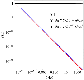
Figure 1: The absolute values of the longitudinal and transverse response functions $|Y_{l}(f)|$ and $|Y_{b}(f)|$ as functions of $f$ for aLIGO to a scalar gravitational wave with the masses $1.2\times 10^{-22}\,\text{eV}/c^{2}$ Abbott et al. (2016a) (dotted blue curve) and $7.7\times 10^{-23}$ eV/$c^{2}$ Abbott et al. (2017a) (dashed red curve). The solid curve denotes $|Y_{b}(f)|$. Taken from Ref. Gong and Hou (2018).

A second method to detect GWs is to use pulsar timing arrays (PTAs) Hellings and Downs (1983); Lee et al. (2008, 2010); Chamberlin and Siemens (2012); Lee (2013); Gair et al. (2014, 2015). The stochastic GW background causes the pulse time-of-arrival (TOA) residuals $\tilde{R}(t)$ from pulsars which can be measured by PTAs Hellings and Downs (1983). The TOA residuals of two pulsars (named $a$ and $b$) are correlated, which is measured by the cross-correlation function $C(\theta)=\langle\tilde{R}_{a}(t)\tilde{R}_{b}(t)\rangle$ with $\theta$ is the angular separation between $a$ and $b$. The brackets indicate the ensemble average over the stochastic background. Figure 2 shows the normalized correlation function $\zeta(\theta)=C(\theta)/C(0)$. The left panel shows $\zeta(\theta)$ induced by the massless field $\tilde{h}_{\mu\nu}$ (the solid black curve) and the massless scalar field $\varphi$ (the dashed blue curve). The right panel displays $\zeta(\theta)$ induced by the mixed polarization of the transverse and longitudinal ones. $\alpha$ is the power-law index Lee et al. (2008). So this result provides the possibility to determine the polarization content of GWs. In Fig. 3, we calculated $\zeta(\theta)$ for the massless (labeled by Breathing) and the massive (5 different masses in units of $m_{b}$) cases. One can find out that $\zeta(\theta)$ induced by $\varphi$ is quite sensitive to small masses with $m\leq m_{b}$, but for larger masses, $\zeta(\theta)$ barely changes.

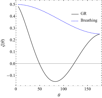
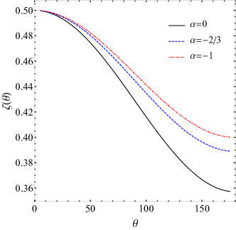
Figure 2: The normalized cross-correlation functions $\zeta(\theta)=C(\theta)/C(0)$. The left panel shows the cross-correlations when the scalar field is massless, i.e., when there is no longitudinal polarization. The solid curve is for the plus or the cross polarizations, and the dashed curve for the transverse breathing polarization. The right panel shows the cross-correlations induced together by the transverse breathing and longitudinal polarizations when the mass of the scalar field is taken to be $m_{b}=7.7\times 10^{-23}\,\mathrm{eV}/c^{2}$. The calculation was done assuming the observation time $T=5$ yrs. Taken from Ref. Hou et al. (2018).

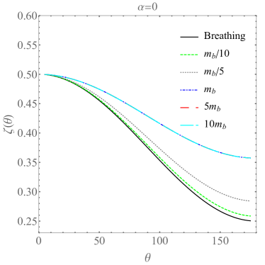
Figure 3: $\zeta(\theta)$ as a function of scalar mass $m$ at $\alpha=0$. The calculations were also done for a 5-year observation. Taken from Ref. Hou et al. (2018).

In our approach, it is not allowed to calculate the cross-correlation function separately for the longitudinal and the transverse polarizations, because they are both excited by the same field $\varphi$ and the polarization state is a single mode.

V Gravitational Wave Polarizations in Einstein-æther Theory and Generalized TeVeS Theory

Finally, we briefly talk about the GW polarization contents in Einstein-æther theory Jacobson and Mattingly (2004) and generalized TeVeS Theory Bekenstein (2004); Seifert (2007); Sagi (2010). There are more d.o.f. in these theories, and they excite more polarizations. These two theories both contain the normalized timelike vector fields, so the local Lorentz invariance is violated. This allows superluminal propagation. Although all polarizations are massless, NP formalism cannot be applied neither. The experimental constraints and the implications for the future experimental tests of these theories can be found in Ref. Gong et al. (2018); Hou and Gong (2018).

V.1 Einstein-æther Theory

Einstein-æther theory contains the metric tensor $g_{\mu\nu}$ and the æther field $u^{\mu}$ to mediate gravity. The action is

$$\begin{split}S_{\text{EH-\ae}}=&\frac{1}{16\pi G}\int\mathrm{d}^{4}x\sqrt{-g}[R-c_{1}(\nabla_{\mu}u_{\nu})\nabla^{\mu}u^{\nu}-c_{2}(\nabla_{\mu}u^{\mu})^{2}-c_{3}(\nabla_{\mu}u_{\nu})\nabla^{\nu}u^{\mu}\\ &+c_{4}(u^{\rho}\nabla_{\rho}u^{\mu})u^{\sigma}\nabla_{\sigma}u_{\mu}+\lambda(u^{\mu}u_{\mu}+1)],\end{split}$$ (42)

where $\lambda$ is a Lagrange multiplier and $G$ is the gravitational coupling constant, the constants $c_{i}\,(i=1,2,3,4)$ are the coupling constants. A special solution solves the equations of motion, i.e., $g_{\mu\nu}=\eta_{\mu\nu}$ and $u^{\mu}=\underline{u}^{\mu}=\delta^{\mu}_{0}$. Linearizing the equations of motion ($g_{\mu\nu}=\eta_{\mu\nu}+h_{\mu\nu}$ and $u^{\mu}=\underline{u}^{\mu}+v^{\mu}$), and using the gauge-invariant variables defined in Ref. Gong et al. (2018), one obtains the following equations of motion

$$\frac{c_{14}}{2-c_{14}}[c_{123}(1+c_{2}+c_{123})-2(1+c_{2})^{2}]\ddot{\Omega}+c_{123}\nabla^{2}\Omega=0,$$ (43)

$$c_{14}\ddot{\Sigma}_{j}-\frac{c_{1}-c_{1}^{2}/2+c_{3}^{2}/2}{1-c_{13}}\nabla^{2}\Sigma_{j}=0,$$ (44)

$$\frac{1}{2}(c_{13}-1)\ddot{h}_{jk}^{\mathrm{TT}}+\frac{1}{2}\nabla^{2}h_{jk}^{\mathrm{TT}}=0,$$ (45)

where $c_{13}=c_{1}+c_{3}$, $c_{14}=c_{1}+c_{4}$, and $c_{123}=c_{1}+c_{2}+c_{3}$. There are five propagating d.o.f., and they propagate at three speeds. The squared speeds are given by

$$s_{g}^{2}=\frac{1}{1-c_{13}},\quad s_{v}^{2}=\frac{c_{1}-c_{1}^{2}/2+c_{3}^{2}/2}{c_{14}(1-c_{13})},\quad s_{s}^{2}=\frac{c_{123}(2-c_{14})}{c_{14}(1-c_{13})(2+2c_{2}+c_{123})}.$$ (46)

These speeds are generally different from each other and the speed of light. In fact, the lack of the gravitational Cherenkov radiation requires them to be superluminal Elliott et al. (2005).

The polarization content can be obtained in terms of the gauge-invariant variables Flanagan and Hughes (2005),

$$R_{tjtk}=-\frac{1}{2}\ddot{h}_{jk}^{\mathrm{TT}}+\dot{\Xi}_{(j,k)}+\Phi_{,jk}-\frac{1}{2}\ddot{\Theta}\delta_{jk}.$$ (47)

Again, assume the GW propagates in the $+z$ direction with the following wave vectors

$$k_{s}^{\mu}=\omega_{s}(1,0,0,1/s_{s}),\quad k_{v}^{\mu}=\omega_{v}(1,0,0,1/s_{v}),\quad k_{g}^{\mu}=\omega_{g}(1,0,0,1/s_{g}),$$ (48)

for the scalar, vector and tensor GWs, respectively. One finds out that there are five polarization states: the plus polarization is represented by $\hat{P}_{+}=-R_{txtx}+R_{tyty}=\ddot{h}_{+}$, and the cross polarization is $\hat{P}_{\times}=R_{txty}=-\ddot{h}_{\times}$; the vector-$x$ polarization is donated by $\hat{P}_{xz}=R_{txtz}\propto\partial_{3}\dot{\Sigma}_{1}$, and the vector-$y$ polarization is $\hat{P}_{yz}=R_{txty}\propto\partial_{3}\dot{\Sigma}_{2}$; the transverse breathing polarization is specified by $\hat{P}_{b}=R_{txtx}+R_{tyty}\propto\dddot{\Omega}$, and the longitudinal polarization is $\hat{P}_{l}=R_{tztz}\propto\dddot{\Omega}$. Note that both the transverse breathing and the longitudinal modes are excited by the same scalar d.o.f. $\Omega$, so $\Omega$ excites a mixed state of $\hat{P}_{b}$ and $\hat{P}_{l}$, as in the case of Horndeski theory Hou et al. (2018); Gong and Hou (2018).

Although the five polarizations are null, the NP formalism cannot be applied, as they propagate at speeds other than 1. Indeed, the calculation showed that none of the NP variables vanish in general.

V.2 Generalized TeVeS Theory

Tensor-Vector-Scalar (TeVeS) theory was the relativistic realization of Milgrom’s modified Newtonian dynamics (MOND) Bekenstein (2004); Milgrom (1983a, b, c). It has an additional scalar field $\sigma$ to mediate gravity. The action for the vector field $u^{\mu}$ is of the Maxwellian form. Later, it was generalized and replaced by the action for the æther field to solve some of the problems that TeVeS theory suffers Seifert (2007). The new theory is simply called the generalized TeVeS theory, whose action includes Eq. (42) and the one for the scalar field,

$$S_{\sigma}=-\frac{8\pi}{\jmath^{2}\ell^{2}G}\int\mathrm{d}^{4}x\sqrt{-g}\mathcal{F}(\jmath\ell^{2}j^{\mu\nu}\sigma_{,\mu}\sigma_{,\nu}),$$ (49)

where $j^{\mu\nu}=g^{\mu\nu}-u^{\mu}u^{\nu}$, $\jmath>0$ is dimensionless and $\ell$ is a constant with the dimension of length. The dimensionless function $\mathcal{F}$ is chosen to produce the relativistic MOND phenomena.

We use the similar method to obtain the polarization content for this theory as for Einstein-æther theory. Since there is one more d.o.f., there is one more polarization state: a mix polarization of the longitudinal and transverse breathing polarizations excited by the new d.o.f. $\sigma$. This polarization state is also massless and propagates at a different speed from 1. So the NP formalism cannot be applied to this theory either.

VI Conclusion

In this talk, we discussed the polarization contents in several alternative theories of gravity: $f(R)$ gravity, Horndeski theory, Einstein-æther theory and generalized TeVeS theory. Each theory predicts at least one extra polarization states due to the extra d.o.f. contained in it. In the case of the local Lorentz invariant theories, such as $f(R)$ gravity and Horndeski theory, the massive scalar field excites a mix of the longitudinal and the transverse breathing polarizations; the massless scalar field excites only the transverse breathing one. In the case of the local Lorentz violating theories, such as Einstein-æther theory and generalized TeVeS theory, each of the scalar d.o.f. is massless, but it propagates at speeds different from 1, so it also excites a mix of the longitudinal and the transverse breathing polarizations. Einstein-æther theory and generalized TeVeS theory also have vector polarizations due to the presence of the vector fields. $E(2)$ classification was designed to categorize the polarizations for the null and Lorentz invariant theories, so it cannot be applied to these theories. The experimental tests of the extra polarizations were also discussed. The analysis showed that the interferometers are not sensitive to the longitudinal polarization which might be detected using PTAs.