Abstract

We study the noise-induced escape from a stable limit cycle of a non-gradient dynamical system driven by a small additive noise. The fact that the optimal transition path in this case is infinitely long imposes a severe numerical challenge to resolve it in the minimum action method. We first consider the landscape of the quasi-potential near the limit cycle, which characterizes the minimal cost of the noise to drive the system far away form the limit cycle. We derive and compute the quadratic approximation of this quasi-potential near the limit cycle in the form of a positive definite solution to a matrix-valued periodic Riccati differential equation on the limit cycle. We then combine this local approximation in the neighbourhood of the limit cycle with the minimum action method applied outside of the neighbourhood. The neighbourhood size is selected to be compatible with the path discretization error. By several numerical examples, we show that this strategy effectively improve the minimum action method to compute the spiral optimal escape path from limit cycles in various systems.

Keywords: rare event, non-gradient system, quasi-potential, limit cycle, minimum action method

Mathematics Subject Classification (2010) Primary 65K05, Secondary 82B05

1. Introduction

Many physical and biological systems exhibit sustainable oscillating dynamics and are altered by random external perturbations simultaneously. To understand the long term impact of noise on the stable oscillations in a deterministic dynamics is an important question. We here consider a continuous-time dynamical system exhibiting a stable limit cycle, subject to the additive random perturbation in the small noise limit. The model is the following Ito stochastic differential equation in $\mathbb{R}^{d}$:

$$\mathrm{d}x_{t}=b(x_{t})\mathrm{d}t+\sqrt{\varepsilon}\sigma(x_{t})\mathrm{d}w_{t},~{}~{}\quad\varepsilon\ll 1,$$ (1)

where $b:\mathbb{R}^{d}\to\mathbb{R}^{d}$ is a smooth drift vector field, $w_{t}$ is the standard $\mathbb{R}^{d}$-valued Wiener process, $\sigma:\mathbb{R}^{d}\to\mathbb{R}^{d}$ is a matrix-valued function and the positive semidefinite matrix $a(x):=\sigma(x)\sigma(x)^{\textsf{T}}$ is usually known as the diffusion tensor. We are concerned with the case that the deterministic dynamical system $\dot{x}=b(x)$ has a stable limit cycle $\Gamma$. This model of noisy perturbed stable oscillations has attracted many interests in the areas of nonlinear oscillators in biology, synchronization of neural network dynamics, fluid dynamics and so on[16, 21, 6, 29, 28, 10]. The central question in concern is how the stochastic trajectory of (1) is driven far away from $\Gamma$ due to the long time effect of the noise. Such non-equilibrium behaviors correspond to many important rare events and the stability problems of the stochastic systems.

It is a classic problem on the exit from a domain in a non-equilibrium system and there are many analytical and experimental studies in physics literature on this topic. The asymptotic analysis works [20, 9, 19, 1] have focused on the exit problem where the basin boundary is a closed curve or an unstable limit cycle. For the case considered here on the noise-induced escape from stable limit cycles, [15] and [17] studied the the invariant measure near the stable limit cycle in small noise intensity limit. With the numerical experiments, [2] is concerned with the optimal trajectories in stochastic continuous dynamical systems and maps. The approach [2] is to study the activation energy by solving the underlying Hamiltonian system, which is equivalent in mathematics to the quasi-potential in our approach here based on the Freidlin-Wentzell large deviation principle.

The large deviation theory provides a useful tool for the noise-induced problems for (1) in the asymptotic regime of small noise. The mathematical theory of Freidlin-Wentzell large deviation principle[13] states that the most probable trajectory of (1) between two given points $a_{1}$ and $a_{2}$ is the minimizer of the Freidlin-Wentzell action functional: the minimizer is called the minimum action path (MAP) [12] and the minimum value of the action is the so called quasi-potential. This theory is also applicable to the transitions from a compact invariant set $K_{1}$ to another set $K_{2}$. The quasi-potential landscape, denoted as $V(x)$, takes the zero value at $K_{1}$ and increases its value away from $K_{1}$, intuitively depicting the cost that the noise has to pay to drive the system to reach the target point. So, the quasi-potential is an important quantity describing the landscape of the minimal action for the escape from $K_{1}$. In the case that $K_{1}$ is a stable limit cycle, the level set of the quasi-potential near this limit cycle is very useful to understand the effect of noise in driving the periodic system (1) in the long run time.

It is shown that $V$ satisfies a Hamilton-Jacobi equation [13]. For planar problems $d=2$, one can numerically solve this Hamilton-Jacobi equation with suitable numerical schemes [7]. In general, this problem has to be solved by the variational approach (the least action principle) rather than the PDE approach. The minimum action method (MAM) and its variants [12, 32, 14, 25, 26] have been developed to directly calculate the minimum action path (MAP). In practice, the MAM works on a path with two fixed endpoints, so it naturally fits the situation where both $K_{1}$ and $K_{2}$ are singletons. But when $K_{1}$ is a continuum set, for instance, a limit cycle $\Gamma$, then the challenge for the transition from $K_{1}$ to $K_{2}$ is that every point in $K_{1}$ is equally important since the quasi-potential is zero everywhere inside $K_{1}$, which usually implies that the actual MAP may have an infinite length. This key fact can also be observed from the underlying Hamiltonian flow. The extremal path, together with its corresponding momentum part, satisfies a Hamiltonian flow. When the momentum term in the Hamiltonian flow vanishes, one has a flow identical to the original dynamics $\dot{x}=b(x)$. So the stable set $K_{1}$ in the original dynamics becomes the $\alpha$-limit set of the extremal escape path with non-vanishing momentum. This suggests that the optimal exit path emitting from the limit cycle has an infinite arc length as $t\to-\infty$.

The numerical challenge in practical computation is that it is not possible to resolve an infinitely long path perfectly. The previous study on the Kuramoto-Sivashinsky equation in [31] is to select an arbitrary point on the travelling wave and use the transition from this point to approximate the transition from the travelling wave. This approach works reasonably well if the main purpose is to explore the high dimensional phase space rather than a pursuit of the precise values of quasi-potential, since the accuracy of the path deteriorates critically only near the limit cycle. In addition, the minimum action obtained in this way depends crucially on the initial guess in the optimization: the more loops around the limit cycle in the initial path, the better accuracy of the numerical results, but the length of the numerical path becomes longer and longer.

In this paper, we propose a new computational strategy of the MAM to adaptively compute the MAP from the limit cycle. Our new method is based on the explicit form of the quadratic approximation of the quasi-potential near the limit cycle. To this end, we construct a small tube around the limit cycle, selected by a given numerical tolerance compatible with the discretization of the path. The MAM is only applied to the outside of this tube and the true path spiralling outward with infinite length is truncated to have a finite length with a new initial point confined on the surface of the tube. To construct the analytic form of the quasi-potential in the tubular neighborhood of the limit cycle, the quasi-potential is approximated by a quadratic form with a $(d-1)\times(d-1)$ positive definite matrix $G$ along the limit cycle. $G$ is computed by solving a periodic Riccati differential equation (PRDE), which is not a challenging numerical problem even for a large dimension $d$. The existence-and-uniqueness condition of the positive definite solution to the PRDE is shown to be closely connected to the linear stability of the limit cycle and the non-degeneracy of the diffusion tensor. If $d=2$, we have the analytic solution of $G$ explicitly. The eigenvalues of $G$ along the limit cycle describe the varying widths of the tubular level set of the quasi-potential; the eigenvectors of $G$ lying in the normal plane of the limit cycle tell us which direction is more preferred (or less preferred) for the stochastic trajectory to depart from the limit cycle. The asymptotic approximation of the quasi-potential can also provide the correct initial values if one want to solve the Hamiltonian system to calculate the quasi-potential along the Hamiltonian trajectory.

In the following, Section 2 will review the basics of several theoretic foundations. Section 3 derives the approximation form of the quasi-potential near the limit cycle. Section 4 is devoted to the Riccati matrix differential equations. Our main numerical method is presented in Section 5, followed by several numerical examples in Section 6. The last section is our conclusive part.

2. Review

2.1. Quasi-potential and minimum action method

Assume $\gamma(\tau)$ is a periodic solution of the deterministic dynamics

$$\dot{x}(\tau)=b(x)$$ (2)

with a least period $\mathcal{T}>0$. Then the trajectory $\Gamma:=\left\{\gamma(\tau):\tau\in[0,~{}\mathcal{T}]\right\}$ in the phase space is a limit cycle. $\Gamma$ is assumed to be stable in the sense which will be specified later. Then the SDE (1) is a random perturbation of (2). We are interested in the quasi-potential for the noise perturbed escape from this stable limit cycle:

$$V(x):=\inf_{T>0}\inf_{\phi(-T)\in\Gamma,\phi(T)=x}S_{T}[\phi],$$ (3)

where the Freidlin-Wentzell action functional $S_{T}$ associated with an interval $[-T,~{}T]$ is defined by

$$S_{T}[\phi]=\frac{1}{2}\int_{-T}^{T}\left\|\dot{\phi}-b(\phi)\right\|^{2}_{a(\phi(\tau))}\mathrm{d}\tau,$$ (4)

for an absolute continuous function $\phi$; otherwise, $S_{T}[\phi]=+\infty$. Here

$$a:=\sigma\sigma^{\textsf{T}},~{}~{}\mbox{ and }~{}~{}\left\|v\right\|_{a}:=\sqrt{v^{\textsf{T}}{a}^{-1}v},~{}~{}\left\langle u,v\right\rangle_{a}:=\left\langle u,a^{-1}v\right\rangle=u^{\textsf{T}}a^{-1}v.$$

Remark 1.

If $a$ is not invertible, then the above action functional is modified as follows

$$S_{T}[\phi]=\frac{1}{2}\inf_{\sigma u=\dot{\phi}-b(\phi)}\int_{-T}^{T}\left\|u\right\|^{2}\mathrm{d}\tau.$$ (5)

The quasi-potential $V(x)\geq 0$ and the equality holds on the limit cycle $\Gamma$. It has been shown [13] that $V$ satisfies the Hamilton-Jacobi equation in the basin of attraction of $\Gamma$:

$$\mathbb{H}(x,\nabla V(x))=0,$$ (6)

where the Hamiltonian

$$\mathbb{H}(x,p):=\left\langle b(x),p\right\rangle+\frac{1}{2}\left\langle p,a(x)p\right\rangle.$$ (7)

The extremal path of the variational problem (3) satisfies the canonical equations of the Hamiltonian system:

$$\begin{cases}\dot{\phi}=\mathbb{H}_{p}(\phi,p)=b(\phi)+a(\phi)p,\\ \dot{p}=-\mathbb{H}_{x}(\phi,p)=-(\partial_{x}b(\phi))^{\textsf{T}}p-\frac{1}{2}\partial_{x}\left\langle p,a(\phi)p\right\rangle.\end{cases}$$ (8)

where $[\partial_{x}b(x)]_{ij}=\left[\partial_{x_{j}}b_{i}(x)\right]$ is the Jacobian matrix of the vector field $b$. Then the quasi-potential along the extremal path $\phi$ can be calculated by

$$V(\phi(t))=\frac{1}{2}\int_{0}^{t}\left\|a(\phi(t^{\prime}))p(t^{\prime})\right\|^{2}_{a}\mathrm{d}t^{\prime}=\frac{1}{2}\int_{0}^{t}\left\langle p(t^{\prime}),a(\phi(t^{\prime}))p(t^{\prime})\right\rangle\mathrm{d}t^{\prime}.$$

If caustic arises, then multiple extremal paths may intersect at some points, and the true value of the quasi-potential $V$ at these focusing points is the minimum of the multiple values arising from the multiple extremal paths.

For the transition path escaping the limit cycle $\Gamma$, the initial condition of (8) should be imposed at $t\to-\infty$ as follows: $\underset{t\to-\infty}{\lim}\mbox{dist}(\phi(t),\Gamma)\to 0$ and $\underset{t\to-\infty}{\lim}p(t)=0.$ “dist” is the Hausdorff distance between two sets. But $\Gamma\cap\left\{\phi(t)\right\}=\emptyset$ for any $t\in\mathbb{R}$. In fact, the extremal path winds around the limit cycle and follows the same rotation direction as $\Gamma$. This means that the extremal path has an infinite length.

The geometric action functional [14] is based on the Maupertuis’s principle [18] and written in terms of an arbitrarily parametrized geometric curve:

$$\hat{S}[\varphi]=\int_{\varphi}\left\langle p,\mathrm{d}\varphi\right\rangle=\int_{\varphi}\left\langle(\dot{\phi}-b(\phi)),\mathrm{d}\varphi\right\rangle_{a}$$ (9)

where the curve $\varphi$ is a geometric description for the time variable function $\phi(t)$. The momentum $p(t)=a(\phi(t))^{-1}\left(\dot{\phi}-b(\phi)\right)$ is related to the quasi-potential by $p(t)=\nabla V(\phi(t)).$ Here $\dot{\phi}(t)$ is the time derivative of $\phi$, which has to be provided additionally in $\hat{S}$. If the path $\varphi$ has a finite length $L$, then it can be parametrized by its arc-length $\varphi(s),-L\leq s\leq 0$. The path then has two parametrized forms: $\phi(t)$ and $\varphi(s)$. The optimal change-of-variable between time $t$ and arc-length $s$ is obtained by Maupertuis’s principle. Equivalently, the result corresponds to the zero-Hamiltonian property, $\mathbb{H}(\varphi,p)=0$, which is further equivalent to the important identity

$$\|{\dot{\phi}\|}_{a}=\left\|b(\phi)\right\|_{a}.$$

So, $\mathrm{d}s/\mathrm{d}t=\frac{\left\|b\right\|_{a}}{\left\|\varphi^{\prime}\right\|_{a}}$, where $\varphi^{\prime}(s)$ is the derivative of $\varphi$ parametrized by the arc-length parameter $s$. The geometric minimum action method [14] (gMAM) is based on this new variational problem of minimizing $\hat{S}$.

The quasi-potential defined in (3) then is equivalent to

$$V(x)=\inf_{L>0}\inf_{{\varphi\in AC[-L,~{}0]}\atop{\varphi(-L)\in\Gamma,\varphi(0)=x}}\hat{S}[\varphi],$$ (10)

where $AC[-L,~{}0]$ denotes the space of absolutely continuous functions on $[-L,~{}0]$. As noted above, since the set $\Gamma$ is a limit cycle, the arc length $L$ of the optimal path is infinite. In numerical computation based on (3) or (10), the path has to be truncated by a finite value of either time $T$ or arc length $L$. Thus, the gMAM inevitably produces truncation errors as any other version of MAM . The tMAM [27, 28, 30] strives to adaptively match the truncation errors with the numerical optimization errors by determining a larger and larger $T$ as the resolution of the path is finer and finer. This method works quite remarkably in practice and we think the same idea can also be applied to the gMAM for the case of infinite arc length $L$. But the numerical stiffness increases with the interval length $T$ (or $L$). Our idea here to avoid this stiffness due to infinite long interval length is to find an approximation to the quasi-potential within a tube $\left\{x:\mbox{dist}(x,\Gamma)\leq\delta\right\}$ and the numerical computation is only applied to the outside of this tube.

2.2. Quadratic approximation of the quasi-potential at stationary points.

The asymptotic idea has been implemented to analyze the Hamiltonian flow (8) around stationary points. We briefly review this result [5] on the approximation of the quasi-potential at a stable stationary point. Assume that the linearized dynamics at a stationary point $x_{*}$ (not necessarily stable) of $b$ is $\dot{x}=Jx$ where $J$ is the Jacobian matrix $\partial_{x}b$ at $x_{*}$. $J$ is assumed to be non-degenerated. Assume that $V(x)=\frac{1}{2}x^{\textsf{T}}Ax$, where $A$ is a symmetric matrix to be determined. Then the zero-Hamiltonian condition $\mathbb{H}(x,\nabla V)=0$ and (8) lead to the matrix equation $AJ+J^{\textsf{T}}A+{A}{aA}=0$. The unique positive definite matrix solution $A$ satisfies $A^{-1}=\int_{0}^{\infty}e^{tJ}ae^{tJ^{\textsf{T}}}\mathrm{d}t$ (where $a$ is valued at $x_{*}$). The tangent flow of the Hamiltonian system (8) in $\mathbb{R}^{2d}$ is then in the following two subspaces: $(\dot{x},\dot{p})=(Jx,0)$ and $(\dot{x},\dot{p})=(-(J+A)x,-J^{\textsf{T}}Ax)$. If $J$ corresponds to a stable fixed point (all eigenvalues have negative real parts), then $A$ is positive definite.

The generalization of this asymptotic analysis to the setting for a stable limit cycle is more complicated than this fixed point case. We first need set up some local curvilinear coordinates around the limit cycle by using a moving affine frame along the limit cycle.

2.3. Linear stability of limit cycle

We review some classic concepts for asymptotic stability of periodic ordinary differential equations in the Floquet theory [8]. Some of them will be used later.

Definition 1.

Let $M(\cdot)\in\mathbb{R}^{n\times n}$ be a $\mathcal{T}$-periodic matrix-valued continuous function. Fix an initial time $\tau_{0}$. $\Phi_{M}(\tau,\tau_{0})$ is called the state transition matrix associated with ${M}(\cdot)$ if it solves the periodic matrix differential equation

$$\begin{cases}\dfrac{\partial}{\partial\tau}\Phi_{M}(\tau,\tau_{0})={M}(\tau)\Phi_{M}(\tau,\tau_{0}),\\ \Phi_{M}(\tau_{0},\tau_{0})=I,\end{cases}$$ (11)

where $I$ is the identity matrix. The monodromy matrix at time $\tau$ is defined as

$$\bar{\Phi}_{M}(\tau):=\Phi_{M}(\tau+\mathcal{T},\tau).$$ (12)

The eigenvalues of the monodromy matrix $\bar{\Phi}_{M}(\tau)$ are independent of $\tau$ because $\bar{\Phi}_{M}(\tau)=\Phi_{M}(\tau,0)\bar{\Phi}_{M}(0)\Phi_{M}^{-1}(\tau,0)$. The eigenvalues of the monodromy matrix $\bar{\Phi}_{M}(\tau)$ are called the characteristic multipliers for the linear $\mathcal{T}$-periodic system $\dot{y}(\tau)=M(\tau)y(\tau)$, or simply the characteristic multipliers of $M(\cdot)$.

Recall that $\gamma(\tau)$ is a $\mathcal{T}$-periodic solution of (2), i.e.,

$$\dot{\gamma}(\tau)=b(\gamma(\tau)).$$ (13)

Linearization of (2) around $\gamma(\tau)$ leads to the following periodic linear system

$$\dot{y}=\partial_{x}b(\gamma(\tau))y.$$ (14)

By differentiating (13), we see that $\dot{\gamma}(\tau)$ is a $\mathcal{T}$-periodic solution of the equation (14). It follows that the linear $\mathcal{T}$-periodic system (14) always has a characteristic multiplier equal to $1$. The stability of the limit cycle is characterized by the other $(d-1)$ characteristic multipliers.

Definition 2.

We say that the limit cycle $\Gamma$, which is the orbit of a $\mathcal{T}$-periodic solution $\gamma(\tau)$ of (2), is asymptotically stable if, except for the trivial characteristic multiplier $1$, the other $d-1$ characteristic multipliers of (14) lie inside the open unit disk in the complex plane.

The asymptotic stability of the limit cycle defined in Definition 2 has the property of asymptotic orbital stability in the sense that any solution of (2) which comes near the limit cycle will tend to the limit cycle as $\tau\to+\infty$. Refer to Theorem 2.2 of Chapter 13 in the textbook [8].

2.4. Curvilinear coordinates

To set up the curvilinear coordinates around the limit cycle $\Gamma$ in $\mathbb{R}^{d}$, we need a moving affine frame along the limit cycle $\Gamma$ in $\mathbb{R}^{d}$, i.e., a collection of $d$ differentiable $\mathcal{T}$-periodic mappings $e_{i}:[0,~{}\mathcal{T}]\longrightarrow\mathbb{R}^{d}$, $0\leq i\leq d-1$, such that for all $\tau\in[0,~{}\mathcal{T}]$, the (column) vector set $\{e_{i}(\tau):0\leq i\leq d-1\}$ forms a basis of $\mathbb{R}^{d}$. Each $e_{i}(\tau)$ may be viewed as a vector field along the limit cycle $\Gamma$. In addition, we set $e_{0}(\tau)$ to be a tangent unit vector field along the limit cycle $\Gamma$, i.e.,

$$e_{0}(\tau)=\lambda(\tau)\dot{\gamma}(\tau),$$ (15)

where a superior dot denotes differentiation with respect to $\tau$, and $\lambda(\tau)$ is a $\mathcal{T}$-periodic nonzero scalar function. To be well-defined, we need assume that $\dot{\gamma}(\tau)$ never vanishes for any $\tau$, which amounts to saying that the vector field $b(x)$ never vanishes on the limit cycle $\Gamma$. Given a moving affine frame $e_{i}(\tau)$, $0\leq i\leq d-1$, the following equations for the derivatives hold:

$$\dot{e}_{j}(\tau)=\sum_{i=0}^{d-1}\omega_{j}^{i}(\tau)e_{i}(\tau),\quad\text{for }0\leq j\leq d-1,$$ (16)

where

$$\omega_{j}^{i}(\tau)=\left\langle e^{i}(\tau),\dot{e}_{j}(\tau)\right\rangle,\quad\text{for }0\leq i,j\leq d-1,$$ (17)

and the (column) vector set $\{e^{i}(\tau):0\leq i\leq d-1\}$ is the reciprocal basis for the basis $\{e_{i}(\tau):0\leq i\leq d-1\}$, that is

$$\left\langle e^{i}(\tau),e_{j}(\tau)\right\rangle=\delta^{i}_{j}:=\begin{cases}1,\quad&\text{if }i=j,\\ 0,&\text{otherwise}.\end{cases}$$ (18)

So, the normal plane of the limit cycle $\Gamma$ is $P(\tau):=\mbox{span}\left\{e^{1}(\tau),\ldots,e^{d-1}(\tau)\right\}=(e_{0}(\tau))^{\perp}=(\dot{\gamma}(\tau))^{\perp}$. Actually this normal plane is the $d-1$ dimensional direct sum of the generalized left eigenspaces for the nontrivial eigenvalues (excluding 1) of the monodromy matrix $\bar{\Phi}_{\partial_{x}b(\gamma(\cdot))}(\tau)$ associated with the Jacobian $\partial_{x}b(\gamma(\tau))$.

Let $E(\tau)=\begin{bmatrix}e_{0}(\tau),&\ldots,&e_{d-1}(\tau)\end{bmatrix}$ denote the $d\times d$ matrix whose columns are the vectors $e_{i}(\tau)$, $0\leq i\leq d-1$. Then its inverse matrix is $E(\tau)^{-1}=\begin{bmatrix}e^{0}(\tau)&\cdots&e^{d-1}(\tau)\end{bmatrix}^{\textsf{T}},$ and (16) can be written in the matrix form

$$\dot{E}(\tau)=E(\tau)\Omega(\tau),$$ (19)

or

$$\Omega(\tau)=E(\tau)^{-1}\dot{E}(\tau).$$ (20)

where the element in the $(i+1)$-th row and $(j+1)$-th column of $\Omega(\tau)$ is $\omega^{i}_{j}(\tau)$.

Remark 2.

If one assumes that the basis $\{e_{i}(\tau):0\leq i\leq d-1\}$ is an orthonormal basis, then $e^{i}(\tau)=e_{i}(\tau)^{\textsf{T}}$ and $\left|e_{i}\right|=1$, $0\leq i\leq d-1$. It follows that $\omega^{i}_{j}=\left\langle e_{i},\dot{e}_{j}\right\rangle$ satisfies

$$\omega_{i}^{j}(\tau)=-\omega_{j}^{i}(\tau),\quad\text{for }0\leq i,j\leq d-1,0\leq\tau\leq\mathcal{T},$$

i.e., $\Omega(\tau)$ is antisymmetric.

Assume $\{\gamma(\tau):0\leq\tau\leq\mathcal{T}\}$ is a curve of order $d$, i.e., for all $\tau$, the $k$-th derivative $\gamma^{(k)}(\tau)$, $1\leq k\leq d$, are linearly independent, then we can construct the moving frame $e_{i}(\tau)$, $0\leq i\leq d-1$ from the derivatives of $\gamma(\tau)$ by using the Gram-Schmidt orthogonalization process. Consequently, the resulting frame $e_{i}(\tau)$, $0\leq i\leq d-1$ satisfies that for every $\tau$, the vector set $\{e_{i}(\tau):0\leq i\leq d-1\}$ forms an orthonormal basis in $\mathbb{R}^{d}$, and in addition, for all $1\leq k\leq d$, the $k$-th derivative $\gamma^{(k)}(\tau)$ of $\gamma(\tau)$ lies in the span of the first $k$ vectors $e_{i}(\tau)$, $0\leq i\leq k-1$. It then follows that $\Omega(\tau)$ is antisymmetric and tridiagonal:

$$\Omega(\tau)=\begin{bmatrix}0&\omega_{1}(\tau)&&0\\ -\omega_{1}(\tau)&\ddots&\ddots&\\ &\ddots&0&\omega_{d-1}(\tau)\\ 0&&-\omega_{d-1}(\tau)&0\\ \end{bmatrix}.$$

The frame $\left\{e_{i}(\tau),0\leq i\leq d-1\right\}$ constructed in this way is called the Frenet frame, and the corresponding equation (16) or (19) is known as the Frenet–Serret formula, and the invariant $\kappa_{i}(\tau):=\omega_{i}(\tau)/\left|\dot{\gamma}(\tau)\right|$ is called the $i$-th curvature of the curve $\gamma(\tau)$ and can be determined by $\left\{e_{i}(\tau):0\leq i\leq d-1\right\}$.

2.5. Gradient form in terms of curvilinear coordinates

Now, equipped with an affine frame $e_{i}(\tau)$, $0\leq i\leq d-1$ defined on the limit cycle $\Gamma$ as stated in §2.4 (without the requirement of orthonormality in Remark 2), we introduce a set of local curvilinear coordinates

$$(\tau,z)\in[0,~{}\mathcal{T})\times\mathbb{R}^{d-1},\quad{\color[rgb]{.75,0,.25}{z=(z^{1},\cdots,z^{d-1})^{\textsf{T}}\in\mathbb{R}^{d-1}}}$$ (21)

in the tubular neighborhood of the limit cycle $\Gamma$ by writing a point $x$ in the neighborhood as

$$x(\tau,z):=\gamma(\tau)+\sum_{j=1}^{d-1}z^{j}e_{j}(\tau)=\gamma(\tau)+\widetilde{E}(\tau)z.$$ (22)

Here the ${d\times(d-1)}$ matrix $\widetilde{E}$ is $\widetilde{E}:=\begin{bmatrix}e_{1}(\tau),&\ldots,&e_{d-1}(\tau)\end{bmatrix}.$ Differentiating (22) with respect to $\tau$ and $z_{i}$ yields

$$\partial_{\tau}x =\biggl{[}\lambda(\tau)^{-1}+\sum_{j=1}^{d-1}z^{j}\omega^{0}_{j}(\tau)\biggr{]}e_{0}(\tau)+\sum_{i,j=1}^{d-1}z^{j}\omega^{i}_{j}(\tau)e_{i}(\tau)$$

$$=\left[\lambda(\tau)^{-1}+\left\langle e^{0}(\tau),\dot{\widetilde{E}}(\tau)z\right\rangle\right]e_{0}(\tau)+\widetilde{E}(\tau)\widetilde{\Omega}(\tau)z,$$

$$\partial_{z^{i}}x =e_{i}(\tau),\quad\text{for }1\leq i\leq d-1.$$

$\widetilde{\Omega}(\tau)$ denotes the $(d-1)\times(d-1)$ submatrix of $\Omega(\tau)$ by deleting the first row and the first column. The Jacobian matrix $\begin{bmatrix}\partial_{\tau}x,&\partial_{z^{1}}x,&\cdots&\partial_{z^{d-1}}x\end{bmatrix}$ at $(\tau,z=0)$ of the mapping defined by (22) is the matrix whose columns are the vectors $\lambda(\tau)^{-1}e_{0}(\tau)$, $e_{1}(\tau)$, $\ldots$, $e_{d-1}(\tau)$, therefore it is non-singular for any $\tau$. So the mapping defined by (22) is a local diffeomorphism and gives a differentiable transformation between the Cartesian coordinates $x$ and the curvilinear coordinates $(\tau,z)$. We now can express the gradient operator $\nabla$ in the curvilinear coordinates. Refer to Proposition (10) in the appendix.

3. Quadratic Approximation of quasi-potential

In this section, we study the quadratic approximation of the quasi-potential $V$ near the limit cycle $\Gamma$. We shall derive a periodic Riccati differential equation (PRDE) on the limit cycle and discuss its theoretic properties and numerical calculations.

3.1. Asymptotic analysis

We choose $\tau$ as the physical time in parametrizing the limit cycle $\Gamma=\left\{\gamma(\tau):0\leq\tau\leq\mathcal{T}\right\}$. The other choice, such as the arc-length parametrization, can be easily transformed from the time-parametrization. The main idea is to write $V(x)$ in terms of the curvilinear coordinate $(\tau,z)$ near $\Gamma$ and apply the Taylor expansion of $V$ around $\Gamma$.

Firstly, we have $V(\tau,z)\geq 0$ and particularly on the limit cycle $V(\tau,z=0)=0$. Therefore $\partial_{z^{i}}V(\tau,0)\equiv 0$, $\forall~{}0\leq i\leq d-1$. Consequently, the Taylor expansion of $V(\tau,z)$ in $z$ at $z=0$ reads

$$\begin{split}V(\tau,z)&=\frac{1}{2}\sum_{i,j=1}^{d-1}z^{i}z^{j}G_{ij}(\tau)+O(\left|z\right|^{3})=\frac{1}{2}{z}^{\textsf{T}}{G(\tau)z}+O(\left|z\right|^{3}),\end{split}$$ (23)

where the $(d-1)\times(d-1)$ symmetric matrix $G(\tau)$ is $G_{ij}(\tau)=\partial^{2}_{z^{i}z^{j}}V(\tau,0)$, which is to be determined. Since

$$\partial_{\tau}V=\frac{1}{2}\left\langle z,\dot{G}(\tau)z\right\rangle+O(\left|z\right|^{3})~{}~{}~{}\mbox{ and }~{}~{}~{}\partial_{z}V=G(\tau)z+O(\left|z\right|^{2}),$$

then from Proposition 10 and $1/(\lambda^{-1}+z)=\lambda+O(z)$, we have

$$\begin{split}\nabla V=~{}&\lambda(\tau)\left(\left\langle z,\left[\frac{1}{2}\dot{G}(\tau)-\widetilde{\Omega}(\tau)^{\textsf{T}}G(\tau)\right]z\right\rangle+O(\left|z\right|^{3})\right)e^{0}(\tau)\\ &+\sum_{i=1}^{d-1}\left[(G(\tau)z)_{i}+O(\left|z\right|^{2})\right]e^{i}(\tau).\end{split}$$ (24)

Secondly, we expand the coefficients $b(x)$ and $a(x)$ in the equation (1) in terms of the curvilinear coordinates $(\tau,z)$. For any $x$ in a neighborhood of $\Gamma$, we write the drift vector

$$b(x)=b\Bigl{(}\gamma(\tau)+\sum_{i=1}^{d-1}z^{i}e_{i}(\tau)\Bigr{)}=\sum_{i=0}^{d-1}B^{i}(\tau,z)e_{i}(\tau),$$ (25)

where by (18) the coefficients are

$$B^{i}(\tau,z):=\left\langle e^{i}(\tau),b(x)\right\rangle,~{}~{}0\leq i\leq d-1.$$

On the limit cycle, we have $b(\gamma(\tau))=\dot{\gamma}(\tau)=\lambda(\tau)^{-1}e_{0}(\tau).$ It follows that $B^{0}(\tau,0)=\lambda(\tau)^{-1}$ and $B^{i}(\tau,0)=0$, $1\leq i\leq d-1$. In addition,

$$\partial_{z^{j}}B^{i}(\tau,0)=\left\langle e^{i}(\tau),\partial_{x}b(\gamma(\tau))e_{j}(\tau)\right\rangle,~{}\quad~{}1\leq i,j\leq d-1.$$ (26)

We denote the right hand side of (26) as the $(i,j)$ entry, $1\leq i,j\leq d-1$, of the $(d-1)$ by $(d-1)$ matrix $\widetilde{J}(\tau)$. Note that $\partial_{x}b(\gamma(\tau))$ is the original Jacobian matrix evaluated on the limit cycle $\Gamma$, and $\widetilde{J}(\tau)$ may be viewed as the Jacobian matrix restricted in the $z$-space. Therefore in the neighborhood of $\Gamma$, we have the expansion

$$B^{0}(\tau,z) =\lambda(\tau)^{-1}+O(\left|z\right|),$$ (27)

$$B^{i}(\tau,z) =\sum_{j=1}^{d-1}z^{j}\partial_{z^{j}}B^{i}(\tau,0)+O(\left|z\right|^{2})$$

$$=(\widetilde{J}(\tau)z)^{i}+O(\left|z\right|^{2}),\quad 1\leq i\leq d-1,$$ (28)

For the diffusion tensor $a(x)$, the approximation is simply

$$a(x)=a\Bigl{(}\gamma(\tau)+\sum_{i=1}^{d-1}z^{i}e_{i}(\tau)\Bigr{)}=a(\gamma(\tau))+O(\left|z\right|).$$ (29)

Then by plugging (25), (27),(28) and (29) into the Hamiltonian in (7), we have that

$$\begin{split}\mathbb{H}(x,\nabla V)=~{}&\left\langle b(x),\nabla V\right\rangle+\frac{1}{2}\left\langle\nabla V,a(x)\nabla V\right\rangle\\ =~{}&\left\langle z,\left[\frac{1}{2}\dot{G}(\tau)-\widetilde{\Omega}(\tau)^{\textsf{T}}G(\tau)\right]z\right\rangle+\sum_{i=1}^{d-1}(G(\tau)z)_{i}(\widetilde{J}(\tau)z)^{i}\\ &+\frac{1}{2}\sum_{i,j=1}^{d-1}(G(\tau)z)_{i}\left\langle e^{i}(\tau),a\bigl{(}\gamma(\tau)\bigr{)}e^{j}(\tau)\right\rangle(G(\tau)z)_{j}+O(\left|z\right|^{3})\\ =~{}&\left\langle z,\left[\frac{1}{2}\dot{G}(\tau)-\widetilde{\Omega}(\tau)^{\textsf{T}}G(\tau)\right]z\right\rangle+\left\langle G(\tau)z,\widetilde{J}(\tau)z\right\rangle\\ &+\frac{1}{2}\left\langle G(\tau)z,\widetilde{A}(\tau)G(\tau)z\right\rangle+O(\left|z\right|^{3}),\end{split}$$

where $\widetilde{A}$ is the positive definite symmetric matrix whose element in the $i$-th row and $j$-th column is given by

$$\left\langle e^{i}(\tau),a\bigl{(}\gamma(\tau)\bigr{)}e^{j}(\tau)\right\rangle,~{}~{}1\leq i,j\leq d-1.$$

$\widetilde{A}$ is the restriction of the original diffusion matrix $a$ in the normal plane $P$. Hence, by (6), equating the terms with the same order $z^{i}z^{j}$ yields the following periodic Riccati differential equation (PRDE)

$$\dot{G}(\tau)-\widetilde{\Omega}(\tau)^{\textsf{T}}G(\tau)-G(\tau)\widetilde{\Omega}(\tau)+G(\tau)\widetilde{J}(\tau)+\widetilde{J}(\tau)^{\textsf{T}}G(\tau)+G(\tau)\widetilde{A}(\tau)G(\tau)=0,$$

i.e.,

$$\dot{G}(\tau)=-{\widetilde{M}}(\tau)^{\textsf{T}}G(\tau)-G(\tau){\widetilde{M}}(\tau)-G(\tau)\widetilde{A}(\tau)G(\tau),$$ (30)

where

$${\widetilde{M}}(\tau):=\widetilde{J}(\tau)-\widetilde{\Omega}(\tau),$$ (31)

is the matrix of size $(d-1)\times(d-1)$. Note that the coefficients ${\widetilde{M}}(\tau)$ and $\widetilde{A}(\tau)$ are both $\mathcal{T}$-periodic. We need to seek a periodic positive definite solution $G(\tau)$ to (30).

When $G$ is found, the quasi-potential at a point $(\tau,z)$ then can be approximated locally by the quadratic form

$$Q(\tau,z):=\frac{1}{2}\left\langle z,G(\tau)z\right\rangle$$

due to (23). Then the momentum $p=\nabla V$ is approximate by $\nabla Q$ when $\left|z\right|\ll 1$ as follows due to (24) and Proposition 10:

$$p(\tau,z) =\nabla V(x)\approx\nabla Q$$

$$=\frac{\left|e_{0}(\tau)\right|}{\left|\dot{\gamma}(\tau)\right|}\left\langle z,\left[\frac{1}{2}\dot{G}(\tau)-\widetilde{\Omega}(\tau)^{\textsf{T}}G(\tau)\right]z\right\rangle e^{0}(\tau)+\sum_{i=1}^{d-1}\left[(G(\tau)z)_{i}\right]e^{i}(\tau).$$ (32)

This may serve as the initial condition for the Hamiltonian system. We can build the MAM by restricting the initial point on the contour near the limit cycle $\left\{(\tau,z):Q(\tau,z)=\delta\right\}$ with a small positive $\delta$. The details are discussed in Section 5.

4. Periodic Differential Riccati Equation

This section is devoted to the study of PRDE (30) derived from the previous section. We investigate the existence and uniqueness of the positive definite solution and the relation to the linear stability of the limit cycle as well as the degeneracy of the diffusion tensor.

4.1. Solutions of the Riccati equation

We first state a theoretical result concerning the existence of the positive definite solution for the Cauchy initial value problem of the PRDE (30).

Proposition 3.

Assume that the initial condition $G(0)=G_{0}$ is symmetric and positive semidefinite. Then the solution of the PRDE (30) exists and is symmetric and positive semidefinite for all $\tau\geq 0$. Furthermore, if $G_{0}$ is positive definite, then so is $G(\tau)$ for all $\tau\geq 0$.

For the proof, refer to Proposition 1.1 in [11]. From Proposition 3, we immediately conclude the following result on periodic positive definite solutions to the PRDE (30).

Corollary 4.

Assume $G(\tau)$ is a $\mathcal{T}$-periodic symmetric solution to the PRDE (30). Then $G(\tau)$ is positive (semi)definite for all $\tau$ if and only if $G(\tau_{0})$ is positive (semi)definite for some $\tau_{0}\in[0,~{}\mathcal{T})$.

Next, we give a sufficient and necessary conditions for the existence and uniqueness of the periodic positive definite solution to the PRDE (30). We start with the connection between the PRDE and the periodic Lyapunov differential equation (PLDE). Assume $G(\tau)$ is nonsingular for all $\tau$ (a sufficient condition is that $G$ is nonsingular at certain $\tau_{0}$). Let $H(\tau):=G^{-1}(\tau)$. Then by (30), $H(\tau)$ solves the following PLDE

$$\dot{H}(\tau)={\widetilde{M}}(\tau)H(\tau)+H(\tau){\widetilde{M}}(\tau)^{\textsf{T}}+\widetilde{A}(\tau).$$ (33)

It is easy to verify that the solution of the PLDE (33) with the initial condition $H(\tau_{0})$ is given by

$$H(\tau)=\Phi_{{\widetilde{M}}}(\tau,\tau_{0})H(0)\Phi_{{\widetilde{M}}}(\tau,\tau_{0})^{\textsf{T}}+W(\tau,\tau_{0}),$$ (34)

where $\Phi_{\widetilde{M}}(\tau,\tau_{0})$ refers to the state transition matrix associated with the $\mathcal{T}$-periodic matrix-valued function $\widetilde{M}(\cdot)$ (see Definition 1) and

$$W(\tau,\tau_{0}):=\int_{\tau_{0}}^{\tau}\Phi_{\widetilde{M}}(\tau,s)\widetilde{A}(s)\Phi_{\widetilde{M}}(\tau,s)^{\textsf{T}}\,\mathrm{d}s.$$ (35)

Before we state our theorem, we need introduce some definitions and results from the control theory [3] of linear periodic ordinary differential equations.

Definition 5.

A pair $(M(\cdot),N(\cdot))$ of $n\times n$ and $n\times m$ real $\mathcal{T}$-periodic matrix-valued functions is called controllable if there exists no left eigenvector $u$ of the monodromy matrix $\bar{\Phi}_{M}(0)$ satisfying the equation $u\,(\Phi_{M}(\tau,0))^{-1}N(\tau)=0$ for all $\tau\in[0,~{}\mathcal{T}]$.

In a special case that the left null space of $N$ is zero, then $(M,N)$ is controllable for any $M$. Note the fact that the left null space of any real matrix $N$ is the same as that of $NN^{\textsf{T}}$, then we have the following useful observation.

Lemma 6.

A pair $(M(\cdot),N(\cdot))$ of $n\times n$ and $n\times m$ real $\mathcal{T}$-periodic matrices is controllable if and only if the pair $(M(\cdot),N(\cdot)N(\cdot)^{\textsf{T}})$ is controllable.

Our main result is the following theorem rigorously connecting the linear stability of the limit cycle to the positive definite solution of the PRDE (30), under the assumption of certain controllability determined by the diffusion tensor $a$. The proof is based on some classical results in [4] and is left in Appendix A.

Theorem 7.

The PRDE (30) admits a unique $\mathcal{T}$-periodic positive definite solution if and only if the following two conditions hold:

1. the limit cycle $\Gamma$ is asymptotically stable;

2. at some $\tau^{\prime}\in[0,~{}\mathcal{T})$, the pair $(\bar{\Phi}_{\widetilde{M}}(\tau^{\prime}),W(\tau^{\prime}+\mathcal{T},\tau^{\prime}))$ is controllable. where $\bar{\Phi}_{{\widetilde{M}}}$ is the monodromy matrix of ${\widetilde{M}}$ and $W$ is defined in (35).

Remark 3.

It is worthy to note that the controllable condition (ii) in Theorem 7 as a sufficient condition requires only the existence of $\tau^{\prime}\in[0,~{}\mathcal{T})$ such that the constant matrix pair fixed at this $\tau^{\prime}$ is controllable. The conclusion in Theorem 7 still holds if condition ($ii$) is replaced by a stronger condition (ii’): $(\bar{\Phi}_{\widetilde{M}}(\cdot),W(\cdot+\mathcal{T},\cdot))$ is controllable, or equivalently (ii”): (${\widetilde{M}}(\cdot),\widetilde{A}(\cdot)$) is controllable. We can obtain a weaker (sufficient) condition here in Theorem 7 due to Proposition 14 in Appendix A.

In view of (35), we immediately have the following corollary.

Corollary 8.

Assume the limit cycle $\Gamma$ is asymptotically stable.

1. If there exists $\tau^{\prime}\in[0,~{}\mathcal{T})$, such that $\widetilde{A}(\tau^{\prime})$ is non-singular, then the PRDE (30) admits a unique $\mathcal{T}$-periodic positive definite solution.

2. If for every point $\gamma(\tau)$ on the limit cycle, $\widetilde{A}(\tau)=0$, then the PRDE (30) does not admit a unique $\mathcal{T}$-periodic positive definite solution.

Since $\widetilde{A}(\tau)$ is the restriction of the positive semidefinite diffusion tensor $a(\gamma(\tau))$ on the normal plane $P(\tau)=(e_{0}(\tau))^{\perp}=\mbox{span}\left\{e^{1}(\tau),\ldots,e^{d-1}(\tau)\right\}$, we have the following proposition.

Proposition 9.

Let $\mathcal{N}(a(\gamma(\tau)))$ and $\mathcal{R}(a(\gamma(\tau)))$ be the null space and the range space of $a(\gamma(\tau))$, respectively.

1. The following conditions are equivalent:

   1. The matrix $\widetilde{A}(\tau)$ is non-singular;

   2. $\mathcal{N}\left(a(\gamma(\tau))\right)\cap P(\tau)=\left\{0\right\}$;

   3. Any nonzero vector $\xi$ in $P(\tau)$ is not in the subspace $\mathcal{N}\left(a(\gamma(\tau))\right)$.

2. The following conditions are equivalent:

   1. The matrix $\widetilde{A}(\tau)=0$;

   2. $P(\tau)\subset\mathcal{N}\left(a(\gamma(\tau))\right)$.

   3. $\mathcal{R}\left(a(\gamma(\tau))\right)\subset\mbox{span}\left\{\dot{\gamma}(\tau)\right\}$.

The proof is trivial and skipped. In Proposition 9, the condition 1.(c) means that any perturbation force in the normal plane should not be nullified by the linear transformation $\xi\to a{\xi}$ in the perturbed system (1). The heuristic argument of 2.(c) is that when $\xi\to\sigma\xi$ (note $\mathcal{R}(a)=\mathcal{R}(\sigma)$) transforms any random force into the tangent direction of the limit cycle, then it is impossible to escape the limit cycle.

4.2. Analytic solution for planar limit cycle

We end this theoretic section with a specific example for $d=2$ where the solution can be obtained explicitly.

In the case $d=2$, the limit cycle $\Gamma$ is a curve in the plane. Let $e_{0}$ be the unit tangent vector $\dot{\gamma}/\left|\dot{\gamma}\right|$ and $e_{1}$ be the unit normal vector $\vec{n}$. It follows that $\widetilde{\Omega}\equiv 0$. The matrix PRDE (30) reduces to a scalar PRDE: $\dot{G}(\tau)=-2{\widetilde{M}}(\tau)G(\tau)-\widetilde{A}(\tau)G(\tau)^{2},$ where $\widetilde{A}(\tau)=\left\langle e_{1},ae_{1}\right\rangle=\left\langle\vec{n},a\vec{n}\right\rangle\geq 0$ is the diffusion coefficient in the normal direction $\vec{n}$ of $\Gamma$, and ${\widetilde{M}}(\tau)=\left\langle\vec{n},(\partial_{x}b)\vec{n}\right\rangle$ is the Jacobian of $b$ along the normal direction $\vec{n}$. It is easy to solve the state transition matrix $\Phi_{\widetilde{M}}(\tau,0)=\exp\left(\int_{0}^{\tau}{\widetilde{M}}(s)\,\mathrm{d}s\right)$ and the solution of the Lyapunov equation:

$$H(\tau)=H(0)\exp\left(2\int_{0}^{\tau}{\widetilde{M}}(s)\,\mathrm{d}s\right)+\int_{0}^{\tau}\widetilde{A}(s)\exp\left(2\int_{s}^{\tau}{\widetilde{M}}(\sigma)\,\mathrm{d}\sigma\right)\,\mathrm{d}s.$$ (36)

The $\mathcal{T}$-periodic solution $H(\tau)$ satisfies $H(0)=H(\mathcal{T})$ and it follows that

$${H(0)}=\frac{\displaystyle\int_{0}^{\mathcal{T}}\widetilde{A}(s)\exp\left(2\int_{s}^{\mathcal{T}}{\widetilde{M}}(\sigma)\,\mathrm{d}\sigma\right)\,\mathrm{d}s}{\displaystyle 1-\exp\left(2\int_{0}^{\mathcal{T}}{\widetilde{M}}(s)\,\mathrm{d}s\right)}.$$ (37)

The periodic solution of the PRDE is $G(\tau)=\frac{1}{H(\tau)}$ with $H$ given by (36).

For this planar case, the condition (i) in Theorem 7 reads $\bar{\Phi}_{\widetilde{M}}(0)=\exp\left(\int_{0}^{\mathcal{T}}{\widetilde{M}}(s)\,\mathrm{d}s\right)<1,~{}\mbox{ i.e.,}~{}\int_{0}^{\mathcal{T}}{\widetilde{M}}(s)\,\mathrm{d}s<0,$ and the condition (ii) amounts to $\widetilde{A}(\tau)\not\equiv 0$. It is easy to see by (37) that these are exactly the sufficient and necessary conditions for $H(0)>0$, in which case we have a unique positive definite solution $G(\cdot)$.

5. Numerical methods

In this section, we develop the related numerical methods for the computation of the quasi-potential and the optimal path escaping from the limit cycle. To find the limit cycle $\Gamma$, we apply the Newton-Raphson method [22]. The Newton-Raphson method can locate the limit cycle with arbitrary accuracy and a convergence rate much faster than integrating the ODE. After the stable limit cycle is found, the first issue is how to robustly generate the moving frame on the limit cycle.

5.1. Construction of the frame vectors

All coefficients of the PRDE (30) for $G$ are based on the matrix $\widetilde{\Omega}$ via the moving frame given by the basis vectors $\left\{e_{j}(\tau):0\leq j\leq d-1,0\leq\tau\leq\mathcal{T}\right\}$. To robustly construct this basis with a good quality is not quite straightforward in high dimension.

The normalization condition $\left|e_{i}(\tau)\right|\equiv 1$ is always enforced and the first vector $e_{0}(\tau)$ is set to be along the tangent direction: $e_{0}:=\dot{\gamma}/\left|\dot{\gamma}\right|$. $d=2$ is a trivial case where $e_{1}$ is simply obtained by rotating $e_{0}$ with the angle $\pi/2$ in the plane. For a general $d$, one could construct a set of orthonormal basis $\left\{e_{j}\right\}$ to have the Frenet frame, by using the time derivatives of $\gamma$ as Remark 2 has shown. But this approach is not practical for high dimension $d$ since it has the numerically instability in computing the high order derivatives $\gamma^{(k)}(\tau)$ for $k$ large. Furthermore, it usually leads to the vectors $\left\{{\color[rgb]{.75,0,.25}{\gamma^{(j)}}}(\tau):1\leq j\leq d\right\}$ close to degeneracy, with a very bad condition number of the resulted matrix $E(\tau)$, even after a low-pass filtering technique applied to the numerical derivatives. Consequently the calculation of the inverse $E^{-1}$ or the Gram-Schmidt orthogonalization becomes impractical even for $d>4$, observed from our numerical experiments. The use of time derivative of $\gamma$ also suffers from the fact that at some point the derivative may be zero. For example, in the plane, a curve can change the rotation from counterclockwise to clockwise and as a result, the signed curvature (the first order derivative of $e_{0}$) is zero at the turning point.

We propose a robust construction of the basis by choosing ${e_{1}(\tau),\ldots,e_{d-1}(\tau)}$ for each $\tau$ as the $d-1$ left-eigenvectors (by excluding the eigenvector associated with the trivial eigenvalue $1$) of the monodromy matrix $\bar{\Phi}_{\partial_{x}b(\gamma)}(\tau)$; refer to Section 2.3. The sign of the eigenvectors $e_{j}(\tau)$ at $\tau>0$ are chosen to be continuous in $\tau$ after the direction at $\tau=0$ is fixed. Then $e_{0}(\tau)$ is always orthogonal to other basis vectors, i.e., the normal plane $P(\tau)$ is $\mbox{span}\left\{e_{1}(\tau),\ldots,e_{d-1}(\tau)\right\}$ for every $\tau$. We do not have that $\left\{e_{1},\ldots,e_{d-1}\right\}$ are orthogonal by themselves. If one uses the right-eigenvectors instead of the left-eigenvectors, then the only difference is the loss of the orthogonality of $e_{0}$ and $\left\{e_{1}(\tau),\ldots,e_{d-1}(\tau)\right\}$.

Our approach has the computational overhead of solving the matrix-valued ODE (11) for each $\tau$ in parallel. But this method is robust and produces better numerical representations of $\widetilde{\Omega}$ and the coefficients $\widetilde{M}$ and $\widetilde{A}$ for PRDE (30), which is critical to solve $G$ successfully in the next step.

5.2. Numerical method for the Riccati equation

We use the iterative method to find the periodic solution $G$ of the PRDE (30). Each iteration $G_{n}\mapsto G_{n+1}$ simply maps a positive definite matrix $G_{n}$ to the solution at time $\mathcal{T}$ of (30) with the initial value $G_{n}$. This method is equivalent to integrate the PRDE (30) in forward time for sufficiently long time, i.e., we seek for a stable limit cycle of the dynamical system (30) in the space of positive definite matrix. The convergence to the positive definite periodic solution is guaranteed [23] if the initial guess $G_{0}$ is sufficiently large. We use a scalar matrix $cI_{d-1}$ with a large $c$ for the initial.

As mentioned before, our basis $\left\{e_{j}\right\}$ is constructed from the eigenvectors of the monodromy matrix. For some examples (see Section 6.4), the eigenvectors may not be periodic, but anti-periodic (a simple analogy is the normal vector of the Möbius band). The anti-periodic situation needs the following special technique of computing $G$ in (30). We assume that the first $d_{+}$ basis vectors are periodic while the last $d_{-}=d-d_{+}$ vectors are anti-periodic. Specifically, we have one basis set with the matrix form

$$E^{+}(\tau)=[e^{+}_{0}(\tau),\ldots,e^{+}_{d-1}(\tau)]$$

where all $e^{+}_{j}(\tau)$ are $C^{1}$ in $[0,\mathcal{T})$, but $e^{+}_{j}(\mathcal{T})=e^{+}_{j}(0)$ for $0\leq j\leq d_{+}-1$ and $e^{+}_{j}(\mathcal{T})=-e^{+}_{j}(0)$ for $d_{+}\leq j\leq d-1$. Then we define the following basis set

$$E^{-}(\tau):=[e^{-}_{0}(\tau),\ldots,e^{-}_{d-1}(\tau)]=E^{+}(\tau)F$$

where $e^{-}_{j}:=e^{+}_{j}$ for $0\leq j\leq d_{+}-1$ and $e^{-}_{j}:=-e^{+}_{j}$ for $d_{+}\leq j\leq d-1$. Equivalently to this definition of new basis set, the $d\times d$ matrix $F$ is $\begin{bmatrix}I_{d_{-}}&0\\ 0&-I_{d_{+}}\end{bmatrix}.$ Correspondingly, we can have $\widetilde{M}^{+}$, $\widetilde{M}^{-}$ and $\widetilde{A}^{+}$, $\widetilde{A}^{-}$, based on these two local coordinate systems $E^{+}$ and $E^{-}$, respectively. We then solve the following $2\mathcal{T}$-periodic Riccati equation for each of the above iterations $G_{n}\mapsto G_{n+1}$:

$$\begin{cases}\dot{G}(\tau)&=-\hat{M}(\tau)^{\textsf{T}}G(\tau)-G(\tau)\hat{M}(\tau)-G(\tau)\hat{A}(\tau)G(\tau),~{}~{}0\leq\tau\leq 2\mathcal{T}\\ G(0)&=G_{n},\end{cases}$$ (38)

where the coefficients are defined by

$$\hat{M}(\tau)=\begin{cases}\widetilde{M}^{+}(\tau)&0\leq\tau\leq\mathcal{T}\\ \widetilde{M}^{-}(\tau)&\mathcal{T}<\tau\leq 2\mathcal{T}\end{cases},~{}~{}\hat{A}(\tau)=\begin{cases}\widetilde{A}^{+}(\tau)&0\leq\tau\leq\mathcal{T}\\ \widetilde{A}^{-}(\tau)&\mathcal{T}<\tau\leq 2\mathcal{T}\end{cases}.$$

$G_{n+1}$ is chosen as $G(2\mathcal{T})$. It is not difficult to show that $G(\tau+\mathcal{T})=FG(\tau)F$ for $\tau\in[0,\mathcal{T}]$. So, $G(\tau+\mathcal{T})$ and $G(\tau)$ have the same eigenvalues and their eigenvectors are connected by the elementary matrix $F$: they are essentially the same solution represented by the two different local coordinate systems $E^{+}$ and $E^{-}$. In other words, the solution of (38) is $2\mathcal{T}$-periodic but its eigenvalues are $\mathcal{T}$-periodic. Any point $x$ near the limit cycle has two representations $(\tau,z^{+})$ or $(\tau,z^{-})$, based on $E^{+}$ or $E^{-}$, with the relation $z^{-}=Fz^{+}$. The quadratic approximation of the quasi-potential at $x$ then also has two equivalent forms: $Q(x)=\frac{1}{2}\left\langle z^{+},G(\tau)z^{+}\right\rangle=\frac{1}{2}\left\langle z^{-},G(\mathcal{T}+\tau)z^{-}\right\rangle$.

5.3. Solving Hamiltonian systems to generate extremal trajectories emitting from limit cycle

Quite like the case of a stable fixed point, one can solve the Hamiltonian ODE (8) near the limit cycle with a pair of the correct initial value on the Lagrangian manifold of the Hamiltonian system. The initial values should be set on the tangent space of the Lagrangian manifold emitting from the limit cycle. Select a tiny value $h>0$ and set the initial condition $\phi(t=0):=\gamma(\tau)+\sum_{i=1}^{d-1}z_{i}e_{i}(\tau)$ with the parameters $(\tau,z)$ on the tube $[0,\mathcal{T})\times(h\mathbb{S}^{d-1})$. The corresponding momentum $p(t=0)=\nabla_{x}Q$ is set by (32). Then the quasi-potential $V$ at the position $\phi(t)$ is obtained by $V(\phi(t))=\frac{1}{2}\left\langle z,G(\tau)z\right\rangle+\frac{1}{2}\int_{0}^{T}\left\langle a(x(t)p(t)),p(t)\right\rangle\mathrm{d}t$. One need scan all initials on the tube to generate Hamiltonian trajectories (instantons) for each of them. So, this approach is preferred for the low dimension $d=2$ or $3$. But the patterns revealed by these instantons are insightful for understanding the exit problem.

5.4. Minimum action method to compute the minimum action path emitting from limit cycle

We next formulate how to use the MAM to compute the minimum action path and quasi-potential away from the limit cycle. The version of MAM we used is gMAM. There are three approaches. The most straightforward one is to directly use any traditional MAM by fixing one end of the path on an arbitrary location of the limit cycle. Since the initial path is constructed as a straight line segment connecting two end points, the choice of this fixed endpoint and the initial path becomes very important and usually this method performs bad with a large error both in the path and in the quasi-potential. The second approach is to confine the end on the limit cycle rather than on a specific location, so that this end point of the path can move along the limit cycle during the minimization procedure. We abbreviate this approach to gMAM-LC. Theoretically, as the number of grid points increases, this approach can find the true path with infinitely long path. In gMAM-LC, one needs to use very long path to get relatively accurate result, since a large part of the path will spiral around the limit cycle but contribute very little to action. We remedy this by introducing the third approach which uses the quadratic approximation of the quasi-potential within a small tubular neighbor of the limit cycle. After splitting the total action as the sum of the action from the limit cycle to the neighbor and the action from the neighbor to the final designated endpoint, one only needs to compute the second part by the MAM. Specifically, we use the following tube with a uniform small radius $h>0$ as the neighbor.

$$\mathcal{A}_{h}=\bigcup_{\tau\in(0,\mathcal{T}]}\left\{x\in\mathbb{R}^{d}:x=\gamma(\tau)+\sum_{i=1}^{d-1}z_{i}e_{i}(\tau),\ \ |z|=\sqrt{\sum_{j=1}^{d-1}z^{2}_{i}}\leq h\right\}.$$

An alternative choice is to use the level set of $\mathcal{Q}_{\delta}=\left\{(\tau,z):Q=\frac{1}{2}z^{\textsf{T}}Gz\leq\delta\right\}$ as neighborhood, which gives a slightly different version of the following constraint problem. So we will not give implementation details of this choice here.

We use the gMAM to calculate the optimal path escaping the limit cycle $\Gamma$ and ending at some point $x$ outside of $\mathcal{A}_{\delta}$. The constraint is that the initial point $\varphi(0)$ lies on the surface of $\mathcal{A}_{\delta}$. By considering the local coordinate $(\tau,z)$ of $\varphi(0)$, we have the following constrained minimization problem:

$$V(x)= \min_{\begin{subarray}{c}\tau\in[0,\mathcal{T}],~{}|z|=h,\\ \varphi\in AC([0,1]),~{}\varphi(1)=x\\ \varphi(0)=\gamma(\tau)+\sum_{i=1}^{d-1}z_{i}e_{i}(\tau)\end{subarray}}\left\{\hat{S}[\varphi]+\frac{1}{2}\left\langle z,G(\tau)z\right\rangle\right\}.$$ (39)

We discretize this optimization problem using a linear finite element approximation to the path $\varphi$, then solve it by a standard optimization software, e.g. the fmincon in MATLAB. To implement the arc-length parametrization, we add equi-arclength constraints on the discretized grid points. Denote the objective function as $F(\varphi,\tau,z)=\hat{S}[\varphi]+\frac{1}{2}\left\langle z,G(\tau)z\right\rangle$. After discretization of $\varphi$ using $N$ linear finite elements, we have

$$F_{N}(\varphi,\tau,z)=\hat{S}_{N}[{\bm{\varphi}}_{N}]+\frac{1}{2}\left\langle z,G(\tau)z\right\rangle.$$ (40)

The discrete gMAM action $\hat{S}_{N}[{\bm{\varphi}}_{N}]$ is given as

$$\hat{S}_{N}[{\bm{\varphi}}_{N}]=\sum_{i=1}^{N}\frac{\left|\varphi_{i}-\varphi_{i-1}\right|(\left|b(\varphi_{i})\right|+\left|b(\varphi_{i-1})\right|)}{2}-\left\langle\varphi_{i}-\varphi_{i-1},\frac{b(\varphi_{i})+b(\varphi_{i-1})}{2}\right\rangle,$$ (41)

where ${\bm{\varphi}}_{N}=\left\{\varphi_{0},\varphi_{1},\ldots,\varphi_{N}\right\}$ and we have assumed that $a$ be identity matrix. The constraints for discretized problem are

$$|z|^{2}-h^{2}=0,$$

$$\gamma(\tau)+\sum_{i=2}^{d}z_{i}e_{i}(\tau)-\varphi_{0}=0,$$

$$|\varphi_{i}-\varphi_{i-1}|^{2}-|\varphi_{i}-\varphi_{i+1}|^{2}=0,\quad i=1,\ldots,N-1.$$

We abbreviate this gMAM approach with local quadratic approximation for quasi-potential near limit cycle to gMAM-LQA. It is easy to see that gMAM-LC can be regarded as a special case of gMAM-LQA with $h=0$. The adaptive choice of the value of $h$ is to set $h\propto 1/N$ to get a second order convergence rate in $N$.

6. Numerical examples

6.1. Van der Pol oscillator

The perturbed system takes the form

$$\left\{\begin{array}[]{lcl}\mathrm{d}{x}&=&y\mathrm{d}t+\sigma_{1}(x,y)\sqrt{\varepsilon}\mathrm{d}w_{t}^{x},\\ \mathrm{d}{y}&=&(-x+(1-x^{2})y)\mathrm{d}t+\sigma_{2}(x,y)\sqrt{\varepsilon}\mathrm{d}w_{t}^{y}.\end{array}\right.$$ (42)

The period of the limit cycle $\Gamma$ in the deterministic dynamics is $6.6633$. We consider the following three cases of the diffusion coefficients $\sigma_{1}$ and $\sigma_{2}$:

1. isotropic noise: $\sigma_{1}=\sigma_{2}\equiv 1$;

2. degenerate noise: $\sigma_{1}\equiv 0,\sigma_{2}\equiv 1$;

3. discontinuous coefficients: $\sigma_{1}(x,y)=\sigma_{2}(x,y)=\begin{cases}1&\mbox{ if }x>0;\\ 0&\mbox{ if }x<0.\end{cases}$

The curvilinear coordinate in representing $G$ is the Frenet frame. For the case (i), we plot the limit cycle and the contours of the approximated quasi-potential in the left panel of Figure 1. It is observed that although the level sets outside of the limit cycle are smooth, the level set with a small value $Q=0.02$ inside the limit cycle presents four kinks. The kinks may come from the breakdown of the asymptotic approximation of the local coordinates or from the caustics of the quasi-potential inside the limit cycle. To explore this issue, we compute the behaviors of extremal paths near the limit cycle by applying the symplectic integrator for the Hamiltonian system as dictated in Section 5.3. The numerical value of Hamiltonian is checked to be smaller than $10^{-7}$. The right panel of Figure 1 shows four extremal paths (projected onto the $\mathbb{R}^{2}$ position space ) emitting from the limit cycle. Two of them start from an interior position and spiral in a quite chaotic way whose final destination is either being trapped inside or leaving the limit cycle. These observations may suggest the multi-valued and self-similar features of the quasi-potential inside the stable limit cycle. The similar behavior is observed[24, 2] for the time inverted Van der Pol where the limit cycle is unstable and the focus inside the limit cycle is linearly stable.

Figure 1. left: The limit cycle (thick solid curve) and two level sets (dashed curves) of the quasi-potential $Q(x)$ corresponding to $Q$ being $0.02$ (blue) and $0.1$ (red), respectively. right: The four extremal paths starting from four initial positions close to limit cycle. The quasi-potential at these initial positions is as small as $10^{-5}$. Two paths (dotted curves) start from the inside of limit cycle (one of them finally spirals out of the domain encircled by the limit cycle) and the other two paths (dashed curves) start outside of the limit cycle. The four short bars indicate the direction of the initial momentums associated with the respective position variables.

Next, we study the effect of the diffusion coefficient by comparing the solution $G$ in the above three cases of diffusion coefficients. We plot in Figure 2 the functions of $G(\tau)$ for the three cases. As expected, the quasi-potential in the case (ii) is larger than the quasi-potential in the case (i) since the dynamics of $x$ component contains no noise in the case (ii). For the case (iii), it is seen that after the diffusion matrix $a=\mbox{diag}\left\{\sigma_{1}^{2},\sigma_{2}^{2}\right\}$ is turned off (the dashed black curve in the figure), the quasi-potential does not become steep immediately: it becomes significantly large only after a short period of “buffering” region (where $\tau$ is roughly $2.5\sim 3.5$ in the figure). In this region, even without the noise, the deterministic dynamics on the limit cycle can still carry the previously perturbed trajectory for a while until the trajectory significantly leaves the limit cycle. When the noise is turned on again we see a sharp decrease of the quasi-potential back to a small value again. Note that the case (ii) and (iii) have the degeneracy of the diffusion matrix $a(\tau)$ at certain points, but it does not affect the existence of the positive solution $G$.

Figure 2. The profiles of $G(\tau)$ v.s $\tau$ for the cases (i), (ii), and (iii). The dashed black segment in the case (iii) corresponds to the location where $\sigma_{1}=\sigma_{2}=0$ (i.e. $x<0$) and the solid black segments on the same curve corresponds to the location where $\sigma_{1}=\sigma_{2}=1$.

We use gMAM with local quadratic approximation for the quasi-potential near limit cycle (abbr. gMAM-LQA) and the gMAM with one end point attached to limit cycle (abbr. gMAM-LC) to calculate the quasi-potential of point $(2,-2.5)$ with respect to the given limit cycle. The results of the minimum action path is given in Fig 3(a). The convergence behavior is given Fig 3(b), where we use the results of gMAM-LQA with 160 elements as reference solution. We observe that while both algorithms have second order convergence, the gMAM-LQA give better results than the gMAM-LQA method, that because the gMAM-LC algorithm spends more grid points near the limit cycle which contribute less action.

(a) The minimum action path from the limit cycle to point $(2,-2.5)$.

(b) The convergences of the MAM-LQA algorithm and gMAM-LC algorithm.

Figure 3. Numerical results of the minimum action methods for the Van der Pol example.

6.2. A planar example

The second example in 2-D is the following system [7]:

$$\left\{\begin{array}[]{lcl}\mathrm{d}{x}&=&(x-x^{3}/3+y-y^{3}/9)\mathrm{d}t+\sqrt{\varepsilon}\mathrm{d}w_{t}^{x}\\ \mathrm{d}{y}&=&(x+0.9)\mathrm{d}t+\sqrt{\varepsilon}\mathrm{d}w_{t}^{y}.\end{array}\right.$$ (43)

This example has two stable limit cycles, separated by a saddle point located at $(-0.9,0.6942)$ and the stable and unstable manifolds of this saddle point. The quasi-potential for this example was calculated by directly solving the 2-D Hamilton-Jacobi partial differential equation [7]. We only compute the quasi-potential around one of the limit cycle on the top whose period is $5.7966$ and use the MAM to calculate the minimal escape action for the transition toward the other limit cycle on the bottom by selecting the final point at the saddle point. Figure (4) plots the $G(\tau)$ and MAP. The minimal action calculated in the previous work [7] is 0.1567. The result of gMAM-LQA algorithm with $N=160$ is 0.1599 with a relative error about $0.1\%$. The minimum action paths obtained using gMAM and gMAM-LQA with different $N$’s are given in Fig 5, in which we observe that the gMAM is trapped in a local minimum.

Figure 4. left: The profile of $G(\tau)$, $0\leq\tau\leq\mathcal{T}$, for the 2D example (43). The $x$ and $y$ components of the limit cycle $\Gamma$ is also shown. right: The numerical MAP (blue curve) from the limit cycle (black) to the saddle point (the marker “$\times$”). The red and yellow curves are, respectively, the unstable and stable manifolds of the saddle point.

(a) gMAM with initial point fixed on the limit cycle using 40 elements.

(b) gMAM with initial point fixed on the limit cycle using 160 elements.

(c) gMAM-LQA using $N=40$ elements.

(d) gMAM-LQA using $N=160$ elements.

Figure 5. The MAP from the limit cycle to the saddle point. The same initial guess is used in all four cases: a straight line connecting the two ends in (A) and (B).

6.3. 3D Lotka-Volterra model

The following randomly perturbed system is the example of 3D Lotka-Volterra model for three species $x=(x_{1},x_{2},x_{3})\in\mathbb{R}^{3}$:

$$\mathrm{d}x_{i}(t)=x_{i}\sum_{j=1}^{3}c_{ij}(1-x_{j})\mathrm{d}t+\sqrt{\varepsilon}\mathrm{d}w_{i}(t).$$ (44)

We set the matrix $C=[c_{ij}]=\begin{bmatrix}2&5&0.5\\ 0.5&1&1.48\\ 1&0.5&1\end{bmatrix}.$ There exist two steady non-negative solutions: $x\equiv 1$ has an one-dimensional stable manifold and an unstable spiral two-dimensional manifold; $x\equiv 0$ is unstable and its three unstable eigenvectors are along three coordinate axes, respectively. Around the spiral saddle point $x\equiv 1$, there is a stable limit cycle $\Gamma$ with the period $6.7965$. The two eigenvalues of $G(\tau)$ are plotted in Figure 6 and they have a large gap, indicating a strong directional preference of the quasi-potential near the limit cycle. This results in a large aspect ratio in the tube corresponding to the level set of $Q(x)=\delta$. Figure 7 plots this tubular surface for $\delta=2\times 10^{-5}$, which visually looks like a ribbon rather than a tube. The numerical MAP calculated by gMAM-LQA from the limit cycle to the state $x\equiv 0$ (extinctions of all species) is also shown in Fig 7.

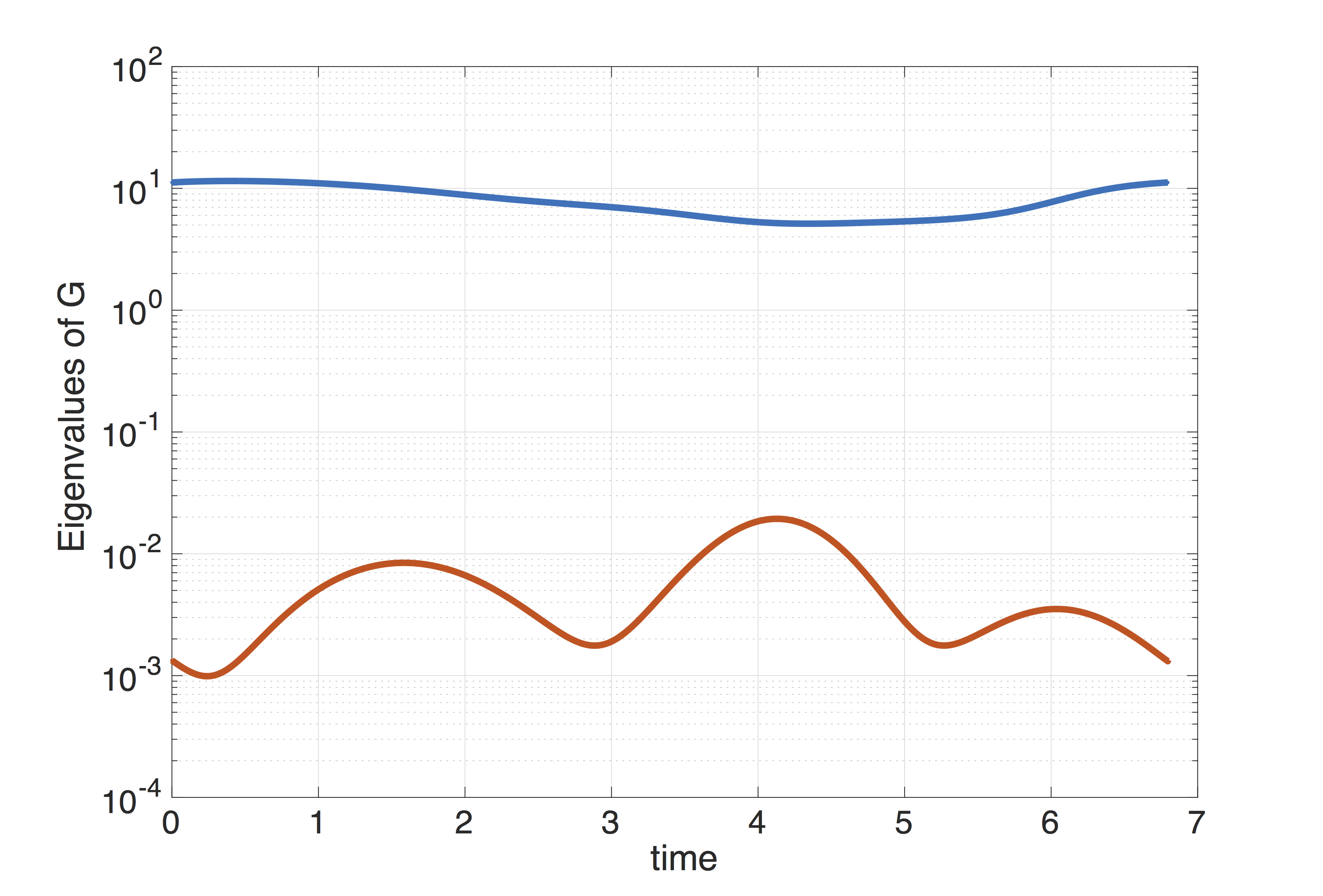
Figure 6. The two eigenvalues of $G$ for the 3D Lotka-Volterra model.

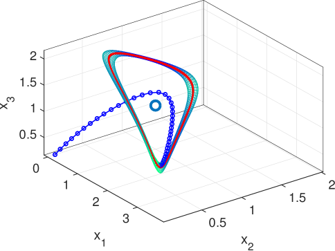
Figure 7. The contour set of the quasi-potential   for the limit cycle of the 3D Lotka-Volterra model (the ribbon-like tube in colors). The MAP from the limit cycle to the unstable point $x\equiv 0$ are plotted as the blue curve with “$\circ$” markers). The isolated large circle is the saddle point $x=(1,1,1)$. A red curve is shown to illustrate the flow of the deterministic flow.

6.4. 5D example

We consider a 5D example whose form is

$$\left\{\begin{array}[]{lcl}\dot{x}_{1}&=&-x_{1}+1-2h(x_{5})-2h(x_{2})+2h(x_{2})h(x_{5})+2h(x_{2})h(x_{4})\\ &&\qquad\qquad-2h(x_{2})h(x_{4})h(x_{5})\\ \dot{x}_{2}&=&-x_{2}+1-2h(x_{1})\\ \dot{x}_{3}&=&-x_{3}+1-2h(x_{2})+2h(x_{2})h(x_{5})\\ \dot{x}_{4}&=&-x_{4}+1-2h(x_{3})\\ \dot{x}_{5}&=&-x_{5}+1-2h(x_{4})-2h(x_{2})+2h(x_{2})h(x_{4})\end{array}\right.$$ (45)

where $h$ is the sigmoid function $h(x)=\frac{1}{2}(1+\tanh(2x))$. The corresponding SDE is to add the isotropic white noise $\sqrt{\varepsilon}\dot{w}_{i}$ to the right hand side of (45). The unique limit cycle is stable with the period $\mathcal{T}=8.1165$. When we constructed the basis $\left\{e_{0},\ldots,e_{4}\right\}$ from the left-eigenvectors of the monodromy matrix, we found that $e_{3}$ and $e_{4}$ are anti-periodic. So we have to solve $G$ by the strategy based on (38) which is introduced in Section 5.2. Figure 8 shows the one-period profile of the component $G_{13}$ during the time interval $(0,2\mathcal{T})$. The eigenvalues of $G$ is $\mathcal{T}$-periodic and we plot the four eigenvalues of $G(\tau),\tau\in[0,\mathcal{T}]$ in the same figure. By using this $G$ and the gMAM-LQA, we compute the MAP from the limit cycle to an endpoint specified at $x=(0.6,0.6,0.7,0.5,0.3)$. Fig 9 demonstrates the projects of this 5 dimensional path.

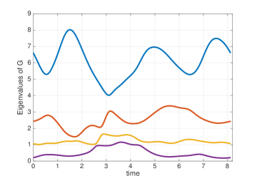
Figure 8. The profile of $(1,3)$ entry of $G(\tau)$, $0\leq\tau\leq 2\mathcal{T}$ and the four eigenvalues of $G$. $\mathcal{T}=8.1165$.

Figure 9. The MAP from the limit cycle to the point $x=(0.6,0.6,0.7,0.5,0.3)$ calculated using gMAM-LQA with $N=40$.

7. Conclusion

We showed how to derive and compute a quadratic approximation of the quasi-potential near a stable limit cycle in random perturbed systems. The minimum action method is improved with the aid of this local approximation to effectively handle the infinite length of the optimal path. With these tools, one can explore the transition behaviors related to stochastic oscillatory in many high dimensional problems.

Appendix A

Proposition 10.

The gradient $\nabla f$ of a differential function $f(x)$, $x\in\mathbb{R}^{d}$, can be written in the curvilinear coordinates as

$$\begin{split}\nabla f(x)&=\frac{\partial_{\tau}f-\sum_{i,j=1}^{d-1}z^{j}\omega^{i}_{j}\partial_{z^{i}}f}{\lambda(\tau)^{-1}+\sum_{j=1}^{d-1}z^{j}\omega^{0}_{j}(\tau)}e^{0}(\tau)+\sum_{i=1}^{d-1}(\partial_{z^{i}}f)e^{i}(\tau)\\ &=\frac{\partial_{\tau}f-\left\langle z,\widetilde{\Omega}(\tau)^{\textsf{T}}\partial_{z}f\right\rangle}{\lambda(\tau)^{-1}+\left\langle e^{0}(\tau),\dot{\widetilde{E}}(\tau)z\right\rangle}e^{0}(\tau)+\sum_{i=1}^{d-1}(\partial_{z^{i}}f)e^{i}(\tau),\end{split}$$

where $\lambda(\tau)$ is defined in (15), $\partial_{z}f$ denotes the column vector whose components are given by $\partial_{z^{i}}f$.

On proof of Theorem 7:

It is clear that a periodic positive definite solution to the PRDE (30) is the inverse of a periodic positive definite solution to the PLDE (33), and vice versa. Hence the proof of Theorem 7 is mainly based on the following classical result on the PLDE. To state this result, we need introduce another type of asymptotical stability for periodic matrix-valued functions.

Definition 11.

Let $M(\cdot)$ be a $\mathcal{T}$-periodic matrix-valued continuous function. We say that $M(\cdot)$ is asymptotically stable if all the characteristic multipliers of $M(\cdot)$ lie inside the open unit disk.

The asymptotical stability of $M(\cdot)$ defined above assures that the periodic linear system $\dot{y}(\tau)=M(\tau)y(\tau)$ has the trivial identically zero solution as an asymptotically stable solution.

In the following proposition, we establish the connection between the two types of asymptotic stability in Definition 11 and Definition 2.

Proposition 12.

${\widetilde{M}}(\cdot)$ defined by (31) is asymptotically stable if and only if the limit cycle $\Gamma$ of (2) is asymptotically stable.

Proof.

We will proof this proposition by showing that the characteristic multipliers associated with (14) consist of 1 and the characteristic multipliers associated with ${\widetilde{M}}(\tau)$, i.e., the eigenvalues of $\bar{\Phi}_{\partial_{x}b(\gamma(\cdot))}(0)$ consist of 1 and the eigenvalues of $\bar{\Phi}_{\widetilde{M}}(0)$.

Let $\Theta(\tau)=E(\tau)^{-1}\Phi_{\partial_{x}b(\gamma(\cdot))}(\tau,0)E(0)$. We claim that $\Theta(\tau)$ is a block upper triangular matrix which has the form $\Theta(\tau)=\begin{bmatrix}\Theta_{11}(\tau)&\Theta_{12}(\tau)\\ 0&\Theta_{22}(\tau)\end{bmatrix},$ where $\Theta_{11}(\tau)$ is a scalar and is equal to $\lambda(0)/\lambda(\tau)$. To see this, we note that the first column of $\Theta(\tau)$ is given by $E(\tau)^{-1}\Phi_{\partial_{x}b(\gamma(\cdot))}(\tau,0)e_{0}(0)$, and the key observation is that

$$\Phi_{\partial_{x}b(\gamma(\cdot))}(\tau,0)e_{0}(0)=\frac{\lambda(0)}{\lambda(\tau)}e_{0}(\tau).$$ (46)

To justify (46), recall that $e_{0}(\tau)=\lambda(\tau)\dot{\gamma}(\tau)$ and $\dot{\gamma}(\tau)$ solves the equation (14) of first variation. Since $\Phi_{\partial_{x}b(\gamma(\cdot))}(\tau,0)$, by definition, is the fundamental matrix solution of (14) and $\Phi_{\partial_{x}b(\gamma(\cdot))}(0,0)=I$, we infer from the uniqueness of the solution to the initial value problem of (14) that

$$\dot{\gamma}(\tau)=\Phi_{\partial_{x}b(\gamma(\cdot))}(\tau,0)\dot{\gamma}(0),$$

and (46) follows immediately.

Next, we will show that $\Theta_{22}(\tau)=\Phi_{{\widetilde{M}}}(\tau,0)$. To this end, we will derive the ODE for $\Theta(\tau)$. Using (19), we have

$$\frac{\mathrm{d}}{\mathrm{d}\tau}E(\tau)^{-1}=-E(\tau)^{-1}\dot{E}(\tau)E(\tau)^{-1}=-\Omega(\tau)E(\tau)^{-1}.$$

Recall that $\Phi_{\partial_{x}b(\gamma(\cdot))}(\tau,0)$ satisfies

$$\frac{\partial}{\partial\tau}\Phi_{\partial_{x}b(\gamma(\cdot))}(\tau,0)=\partial_{x}b(\gamma(\tau))\Phi_{\partial_{x}b(\gamma(\cdot))}(\tau,0).$$

Hence we find

$$\dot{\Theta}(\tau) =-\Omega(\tau)E(\tau)^{-1}\Phi_{\partial_{x}b(\gamma(\cdot))}(\tau,0)E(0)+E(\tau)^{-1}\partial_{x}b(\gamma(\tau))\Phi_{\partial_{x}b(\gamma(\cdot))}(\tau,0)E(0)$$

$$=-\Omega(\tau)\Theta(\tau)+E(\tau)^{-1}\partial_{x}b(\gamma(\tau))E(\tau)\Theta(\tau)$$

$$=M(\tau)\Theta(\tau),$$ (47)

where $M(\tau):=E(\tau)^{-1}\partial_{x}b(\gamma(\tau))E(\tau)-\Omega(\tau).$ Comparing the last equation with (31), we see that ${\widetilde{M}}(\tau)$ is the principal submatrix of $M(\tau)$ by deleting the first row and the first column. Partition $M(\tau)$ into blocks that are compatible with the partitions of $\Theta(\tau)$ and then (47) can be written in the blocked form as

$$\begin{bmatrix}\dot{\Theta}_{11}(\tau)&\dot{\Theta}_{12}(\tau)\\ 0&\dot{\Theta}_{22}(\tau)\end{bmatrix}=\begin{bmatrix}M_{11}(\tau)&M_{12}(\tau)\\ M_{21}(\tau)&{\widetilde{M}}(\tau)\end{bmatrix}\begin{bmatrix}\Theta_{11}(\tau)&\Theta_{12}(\tau)\\ 0&\Theta_{22}(\tau)\end{bmatrix}$$

$$=\begin{bmatrix}M_{11}(\tau)\Theta_{11}(\tau)&M_{11}(\tau)\Theta_{12}(\tau)+M_{12}(\tau)\Theta_{22}(\tau)\\ M_{21}(\tau)\Theta_{11}(\tau)&M_{21}(\tau)\Theta_{12}(\tau)+{\widetilde{M}}(\tau)\Theta_{22}(\tau)\end{bmatrix}.$$

Since $\Theta_{11}(\tau)=\lambda(0)/\lambda(\tau)\neq 0$, we deduce that $M_{21}(\tau)=0$ and then it follows that $\dot{\Theta}_{22}(\tau)={\widetilde{M}}(\tau)\Theta_{22}(\tau).$ Also, we have $\Theta(0)=E(0)^{-1}\Phi_{\partial_{x}b(\gamma(\cdot))}(0,0)E(0)=I$, so $\Theta_{22}(\tau)$ is a $(d-1)\times(d-1)$ identity matrix. Again, by the uniqueness of the solution to the initial value problem, we obtain $\Theta_{22}(\tau)=\Phi_{{\widetilde{M}}}(\tau,0)$.

Since $\lambda(\tau)$ and $E(\tau)$ are $\mathcal{T}$-periodic, we have

$$\Theta(\mathcal{T})=E(\mathcal{T})^{-1}\Phi_{\partial_{x}b(\gamma(\cdot))}(\mathcal{T},0)E(0)=E(0)^{-1}\bar{\Phi}_{\partial_{x}b(\gamma(\cdot))}(0)E(0),$$

and

$$\Theta(\mathcal{T})=\begin{bmatrix}\lambda(0)/\lambda(\mathcal{T})&\Theta_{12}(\mathcal{T})\\ 0&\Phi_{{\widetilde{M}}}(\mathcal{T},0)\end{bmatrix}=\begin{bmatrix}1&\Theta_{12}(\mathcal{T})\\ 0&\bar{\Phi}_{{\widetilde{M}}}(0)\end{bmatrix}.$$

From the last two equations, we conclude that $\bar{\Phi}_{\partial_{x}b(\gamma(\cdot))}(0)$ and $\Theta(\mathcal{T})$ have the same eigenvalues since they are similar, and the eigenvalues of $\Theta(\mathcal{T})$ consist of 1 and the eigenvalues of $\bar{\Phi}_{\widetilde{M}}(0)$. This justifies what we asserted and the proof is complete. ∎

Remark 4.

In Definition 2, the asymptotical stability of the limit cycle $\Gamma$ is clearly defined without using the moving affine frame $e_{i}(\tau)$, $0\leq i\leq d-1$. Thus in view of Proposition 12, the asymptotical stability of ${\widetilde{M}}(\cdot)$ is also a property independent of the choice of the moving affine frame $e_{i}(\tau)$, $0\leq i\leq d-1$, although the matrix ${\widetilde{M}}(\cdot)$ defined by (31) depends explicitly on the moving affine frame $e_{i}(\tau)$, $0\leq i\leq d-1$.

Now Theorem 7 can be easily derived from Proposition 12, Lemma 6 and the following classical results [4].

Proposition 13 (Theorem 20 in [4]).

For any $\mathcal{T}>0$, let $M(\cdot)$, $N(\cdot)$ be two $\mathcal{T}$-periodic matrix-valued functions with size $n\times n$ and $n\times m$ respectively. Then the following PLDE

$$\dot{P}(\tau)=M(\tau)P(\tau)+P(\tau)M(\tau)^{\textsf{T}}+N(\tau)N(\tau)^{\textsf{T}}$$

admits a unique $\mathcal{T}$-periodic positive definite solution $P(\tau)$ if and only if the following two conditions hold:

1. $M(\cdot)$ is asymptotically stable;

2. $(M(\cdot),N(\cdot))$ is controllable.

Proposition 14 (Proposition 9 in [4]).

Let $M(\cdot)$, $N(\cdot)$ be given $n\times n$, $n\times m$ $\mathcal{T}$-periodic matrices respectively. For any $\tau_{0}\in[0,\mathcal{T})$, let ${D}(\tau_{0})$ be a matrix such that

$${D}(\tau_{0}){D}(\tau_{0})^{\textsf{T}}=\int_{\tau_{0}}^{\tau_{0}+\mathcal{T}}\Phi_{M}(\tau_{0}+\mathcal{T},s)N(s)N(s)^{\textsf{T}}\Phi_{M}(\tau_{0}+\mathcal{T},s)^{\textsf{T}}\,\mathrm{d}s.$$

Then the pair $(M(\cdot),N(\cdot))$ is controllable if and only if the time-invariant pair $(\bar{\Phi}_{M}(\tau_{0}),{D}(\tau_{0}))$ is controllable.

References

- [1] N. Berglund and B. Gentz, On the noise-induced passage through an unstable periodic orbit I : Two-level model, J. Stat. Phys, 114 (2004), pp. 1577–1618.
- [2] S. Beri, R. Mannella, D. G. Luchinsky, A. N. Silchenko, and P. V. E. McClintock, Solution of the boundary value problem for optimal escape in continuous stochastic systems and maps, Phys. Rev. E, 72 (2005), p. 036131.
- [3] S. Bittanti, Deterministic and stochastic linear periodic systems, in Time Series and Linear Systems, S. Bittanti, ed., Lecture Notes in Control and Information Sciences, Springer-Verlag, Berlin, New York, 1986, pp. 141–182.
- [4] P. Bolzern and P. Colaneri, The periodic Lyapunov equation, SIAM J. MATRIX ANAL. APPL., 9 (1988), pp. 499–512.
- [5] F. Bouchet, K. Gawedzki, and C. Nardini, Perturbative calculation of quasi-potential in non-equilibrium diffusions: a mean-filed example, Journal of Statistical Physics, 163 (2015), pp. 1157–1210.
- [6] P. C. Bressloff, Stochastic processes in cell biology, vol. 41, Springer, 2014.
- [7] Cameron, M K, Finding the quasipotential for nongradient SDEs, Physica D, 241 (2012), pp. 1532–1550.
- [8] E. A. Coddington and N. Levinson, Theory of Ordinary Differential Equations, McGraw-Hill, 1955.
- [9] M. V. Day, Exit cycling for the van de pol oscillattor and quasipotential calculations, unpublished, (1993).
- [10] R. de la Cruz, R. Perez-Carrasco, P. Guerrero, T. Alarcon, and K. M. Page, Minimum action path theory reveals the details of stochastic transitions out of oscillatory states, Phys. Rev. Lett., 120 (2018), p. 128102.
- [11] L. Dieci and T. Eirola, Positive definiteness in the numerical solution of Riccati differential equations, Numer. Math., 67 (1994), pp. 303–313.
- [12] W. E, W. Ren, and E. Vanden-Eijnden, Minimum action method for the study of rare events, Comm. Pure Appl. Math., 57 (2004), pp. 637–656.
- [13] M. I. Freidlin and A. D. Wentzell, Random Perturbations of Dynamical Systems, Grundlehren der mathematischen Wissenschaften, Springer-Verlag, New York, 3 ed., 2012.
- [14] M. Heymann and E. Vanden-Eijnden, The geometric minimum action method: a least action principle on the space of curves, Comm. Pure Appl. Math., 61 (2008), pp. 1052–1117.
- [15] C. J. Holland, Stochastically perturbed limit cycles, J. Appl. Prob., 15 (1978), pp. 311–320.
- [16] Y. Kuramoto, Nonlinear Oscillations, Dynamical Systems, and Bifurcation of Vecor Fields, Springer-Verlag, Tokyo, 1984.
- [17] C. Kurrer and K. Schulten, Effect of noise and perturbations on limit cycle systems, Physica D: Nonlinear Phenomena, 50 (1991), pp. 311 – 320.
- [18] L. Landau and E. Lifshitz, Mechanics, Course of Theoretical Physics, Butterworth-Heinemann, 3rd ed., 1976.
- [19] R. S. Maier and D. L. Stein, Oscillatory behavior of the rate of escape through an unstable limit cycle, Phys. Rev. Lett., 77 (1996), pp. 4860–4863.
- [20] B. J. Matkowsky and Z. Schuss, Diffusion across characteristic boundaries, SIAM J. Appl. Math., 42 (1982), p. 822.
- [21] F. Moss and P. V. E. McClintock, Noise in Nonlinear Dynamical Systems, vol. 3, Cambridge University Press, 1989.
- [22] T. Parker and L. Chua, Practical numerical algorithms for chaotic systems, Springer-Verlag, 1989.
- [23] M. A. Shayman, On the phase portrait of the matrix riccati equation arising from the periodic control problem, SIAM Journal on Control and Optimization, 23 (1985), pp. 717–751.
- [24] V. N. Smelyanskiy, M. I. Dykman, and R. S. Maier, Topological features of large fluctuations to the interior of a limit cycle, Phys. Rev. E, 55 (1997), pp. 2369–2391.
- [25] E. Vanden-Eijnden and M. Heymann, The geometric minimum action method for computing minimum energy paths, J. Chem. Phys., 128 (2008), p. 061103.
- [26] X. Wan, An adaptive high-order minimum action method, Journal of Computational Physics, 230 (2011), pp. 8669 – 8682.
- [27] X. Wan, A minimum action method with optimal linear time scaling, Communications in Computational Physics, 18 (2015), pp. 1352–1379.
- [28] X. Wan and H. Yu, A dynamic-solver-consistent minimum action method: With an application to 2d Navier-Stokes equations, Journal of Computational Physics, 331 (2017), pp. 209–226.
- [29] X. Wan, H. Yu, and W. E, Model the nonlinear instability of wall-bounded shear flows as a rare event: a study on two-dimensional Poiseuille flow, Nonlinearity, 28 (2015), p. 1409.
- [30] X. Wan, H. Yu, and J. Zhai, Convergence analysis of a finite element approximation of minimum action methods, arXiv:1710.03471 [math], to appear on SIAM J. Numer. Anal. 2018, (2017).
- [31] X. Wan, X. Zhou, and W. E, Study of noise-induced transition and the exploration of the configuration space for the Kuromoto-Sivachinsky equation using the minimum action method, nonlinearity, 23 (2010).
- [32] X. Zhou, W. Ren, and W. E, Adaptive minimum action method for the study of rare events, J. Chem. Phys., 128 (2008), p. 104111.