Focused Hierarchical RNNs for Conditional Sequence Processing

Abstract

Recurrent Neural Networks (RNNs) with attention mechanisms have obtained state-of-the-art results for many sequence processing tasks. Most of these models use a simple form of encoder with attention that looks over the entire sequence and assigns a weight to each token independently. We present a mechanism for focusing RNN encoders for sequence modelling tasks which allows them to attend to key parts of the input as needed. We formulate this using a multi-layer conditional sequence encoder that reads in one token at a time and makes a discrete decision on whether the token is relevant to the context or question being asked. The discrete gating mechanism takes in the context embedding and the current hidden state as inputs and controls information flow into the layer above. We train it using policy gradient methods. We evaluate this method on several types of tasks with different attributes. First, we evaluate the method on synthetic tasks which allow us to evaluate the model for its generalization ability and probe the behavior of the gates in more controlled settings. We then evaluate this approach on large scale Question Answering tasks including the challenging MS MARCO and SearchQA tasks. Our models shows consistent improvements for both tasks over prior work and our baselines. It has also shown to generalize significantly better on synthetic tasks as compared to the baselines.

1 Introduction

Recurrent Neural Networks (RNNs) with attention are wildly used for many sequence modeling tasks, such as: image captioning (Yao et al., 2016; Lu et al., 2017), speech recognition (Chan et al., 2016; Bahdanau et al., 2016), text summarization (Nallapati et al., 2016) and Question and Answering (QA) (Kadlec et al., 2016). The attention mechanism allows the model to look over the entire sequence and pick up the most relevant information. This not only allows the model to learn a dynamic summarization of the input sequence, it allows gradients to be passed directly to the earlier time-steps in the input sequence, which also helps with the vanishing and exploding gradient problem (Hochreiter, 1991; Bengio et al., 1994; Hochreiter, 1998).

Most of these models use a simple form of encoder with attention that is identical to the first one proposed (Bahdanau et al., 2015), where the attention looks over the entire encoded sequence and assigns a soft weight to each token. However, for more complex tasks we conjecture that more structured encoding mechanisms may help the attention to more effectively identify and selectively process relevant information within the input.

Imagine reading a Wikipedia article and trying to identify information that is relevant to answering a question before one knows what the question is. Now, compare this to the situation where the context or question is given before reading the article. It would be much easier to read over the article, identify relevant information, group items and selectively process relevant information based on its relevance to a given context or question.

Keeping this intuition in mind, we have developed a focused RNN encoder that is modeled by a multi-layer RNN that groups input sub-sequences based on gates that are controlled or conditioned on a question or input context. We dub the core part of the minimal form of this model a focused hierarchical encoder module. Our approach represents a general framework that applies to many sequence modeling tasks where the context or question can be beneficial to focus (attend) over the input sequence. Our focused encoder module examined here is based on a two layer LSTM where the upper layer is updated when a group of relevant tokens has been read. The boundaries of the group are computed using a discrete gating mechanism that takes as input the lower and upper level units as well as the context or question, and it is trained using policy gradient methods.

We evaluate our model on several tasks of different levels of complexity. We began with toy tasks with limited vocabulary size, where we analyze the performance, the generalization ability as well as the gating and the attention mechanisms. We then move on to challenging large scale QA tasks such as MS MARCO (Nguyen et al., 2016) and SearchQA (Dunn et al., 2017). Our model outperforms the baseline for both tasks. For the SearchQA task, it significantly outperforms recently proposed methods (Buck et al., 2018).

The key contributions of our work are the following:

• We explore the use of a conditional discrete stochastic boundary gating mechanism that helps the encoder to focus on parts relevant to the context, we use a soft attention to look over the relevant states.

• We use a reinforcement learning approach to learn the boundary gating mechanism.

• The elements above form the building blocks of our proposed focused hierarchical encoder module, we examine its properties with synthetic data experiments and we show the benefits of using it for QA tasks.

Our model takes an input sequence, a question or context sequence and generates an answer. It can be applied to any sequence tasks where the context or question is beneficial to modulating the processing of an input sequence.

2 Focused Hierarchical RNN

2.1 Architecture

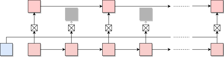
Figure 1: A visualization of FHE. Lower-Layer LSTM processes each step. For each token, the boundary gate decides (based on the current lower-layer LSTM state and question embedding) if information should be stored in the upper-level representation. Higher-Layer LSTM states update only when the corresponding gate is open.

Our model consists of: the focused hierarchical encoder (FHE), the context encoder and the decoder. Compared to a regular RNN with attention, we replace the encoder with a context-aware focused RNN encoder.

The focused hierarchical encoder is modeled by a two-layer LSTM. The lower layer operates at the input token level, while the upper layer focuses on tokens relevant to the context. We train a conditional boundary gate to decide, depending on the context or question, whether it is useful to update the upper-level LSTM with a summary of the current set of tokens or not.

Lower-level Layer

As shown in Figure 1, FHE has two layers. Let $P=(\mathbf{x}_{1},\ldots,\mathbf{x}_{n})$ be the sequence of input tokens, $h_{t}$ be the LSTM hidden state and $c_{t}$ be the LSTM cell state at time $t$. To make our model as generic as possible, the lower-level layer may be also augmented with other available information. The question for large QA tasks are non-trivial and hence we augment the lower-layer inputs with the question encoding at each step.

$$\mathbf{h}_{t}^{l},\mathbf{c}_{t}^{l}=\textmd{LSTM}(\mathbf{x}_{t},\mathbf{h}^{l}_{t-1},\mathbf{c}^{l}_{t-1})$$ (1)

Conditional Boundary Gate

For each token in the passage, the boundary gate decides if information at the current time step should be stored in the upper-level representation. We hypothesize that the question is essential in deciding how to represent the passage. To capture this dependency, the boundary gate computation is conditioned on the question embedding $\mathbf{q}$. The question embedding can vary in complexity depending on the difficulty of the task. In the simplest setting, the question embedding is simply a retrieved vector.

The output of the boundary gate is a scalar $b_{t}\in(0,1)$ that is taken to be the parameter of a Bernoulli distribution $\tilde{b}_{t}\sim\textmd{Bernoulli}(b_{t})$ that regulates the gate’s opening at time step $t$. In the simplest case, the boundary gate forward pass is formulated as

$$b_{t}=\sigma(\mathbf{w}_{b}^{\top}\,\textmd{LReLU}(\mathbf{W}_{b}\mathbf{z}_{t}+\mathbf{b}_{b})),$$ (2)

where $\mathbf{W}_{b}$, $\mathbf{b}_{b}$ and $\mathbf{w}_{b}$ are trainable weights, $\textmd{LReLU}(\cdot)$ is a leaky ReLU activation, and $\mathbf{z}_{t}$ is the input that varies and depends on the task. In our experiments we used the following input

$$\mathbf{z}_{t}=[\mathbf{q}\odot\mathbf{h}^{l}_{t},\mathbf{h}^{l}_{t},\mathbf{q}],$$ (3)

where $\odot$ is the element-wise product. Hence, we essentially use three groups of features: question representation multiplied with lower-layer hidden states, question, and lower-layer representations. These three groups are concatenated together and passed through an MLP to yield boundary gate decisions (i.e., open/close).

In a more complex task that has stronger dependency on the upper-level hidden states (see the following paragraph), these can also be used to augment the boundary gate input $\mathbf{z}_{t}$.

Upper-level Layer

The upper-layer LSTM states (denoted $\mathbf{h}_{t}^{u}$) update only when the corresponding lower-layer boundary gate is open.

$$\mathbf{\tilde{h}}_{t}^{u},\mathbf{\tilde{c}}_{t}^{u} = \textmd{LSTM}(\mathbf{h}^{l}_{t},\mathbf{h}^{u}_{t-1},\mathbf{c}^{u}_{t-1})$$ (4)

$$\tilde{b}_{t} \sim \textmd{Bernoulli}(b_{t})$$ (5)

$$\mathbf{c}^{u}_{t} = \tilde{b}_{t}\mathbf{\tilde{c}}_{t}^{u}+(1-\tilde{b}_{t})\mathbf{c}_{t-1}^{u}$$ (6)

$$\mathbf{h}^{u}_{t} = \tilde{b}_{t}\mathbf{\tilde{h}}_{t}^{u}+(1-\tilde{b}_{t})\mathbf{h}_{t-1}^{u}$$ (7)

Final Output

The final output of FHE is a sequence of lower-level states $H^{l}=\{\mathbf{h}^{l}_{1},\ldots,\mathbf{h}^{l}_{n}\}$ and a sequence of upper-level states $H^{u}=\{\mathbf{h}^{u}_{1},\ldots,\mathbf{h}^{u}_{n}\}$, where only $k$ of them are unique and $k=\sum_{t}\tilde{b}_{t}$, the number of times the boundary gates open over the length of the document. The upper-level states $H^{u}$ are typically the only ones being processed by the downstream modules. Hence, all downstream operations are performed faster than if they had to process $H^{l}$ (the effective size of $H^{u}$ is smaller than the size of $H^{l}$).

2.2 Training

We train our model to maximize the log-likelihood of the answer ($A$) given the context ($Q$) and the passage ($P$), using the output probabilities given by our answer decoder:

$$\mathcal{R}=\log p(A\mid Q,P).$$ (8)

Policy Gradient

The discrete decisions involved in sampling the boundary variable $\tilde{b}_{t}$ make it impossible to use standard gradient back-propagation to learn the parameters of the boundary gate. We instead apply REINFORCE-style estimators (Williams, 1992). Denote by $\pi_{b}$ the model policy over the binary vector of decisions $\mathbf{b}=\{\tilde{b}_{1},\ldots,\tilde{b}_{n}\}$. We need to take the derivative:

$$\sum_{\mathbf{b}}\nabla\pi_{b}(\mathbf{b})\mathcal{R}_{\mathbf{b}}=E_{\mathbf{b}\sim\pi_{b}}[\nabla\log\pi_{b}(\mathbf{b})\mathcal{R}_{\mathbf{b}}],$$ (9)

where the reward $\mathcal{R}_{\mathbf{b}}$ can be formulated differently depending on the task. In our synthetic experiments (Section 4), we let $\mathcal{R}_{\mathbf{b}}=\frac{\partial h^{u}}{\partial\tilde{b}_{t}}$. For large scale natural language QA tasks (Section 5), we use $\mathcal{R}_{\mathbf{b}}=\log p(A\mid Q,P,\mathbf{b})$. The aforementioned gradient can be approximated by sampling from the policy $\pi_{b}$ and computing the corresponding terms.

Rewards

We use the final reward $\mathcal{R}_{\mathbf{b}}$ for each decision in the sequence. Following previous work (Williams, 1992; Andrychowicz & Kurach, 2016), we add an exploration term $\alpha H(\pi_{b})$ that prevents the policy from collapsing too soon during training. The $\alpha$ is a hyperparameter to be set.

Sparsity Constraints

We add a constraint on the sparsity of the upper-level representations. We want the model to avoid grouping each token on its own and storing information at each step on the upper level (i.e., always opening the boundary gates). As a remedy we add a small penalty $G(\mathbf{b})$ the model needs to pay for storing information at the upper level. In practice, we found the following formulation to work the best:

$$\beta G(\mathbf{b})=\beta ReLU\left(\big{(}\sum_{t=1}^{T}{b}_{t}\big{)}-\gamma T\right)$$ (10)

where $\beta>0$ and $\gamma\in[0,1)$ are hyper-parameters and $T$ is the input sequence length. Hence, $\beta$ is the strength of penalty and $\gamma$ is the proportion of the time the gates could open without being penalized. Intuitively, we let a certain number of gates until a open threshold $\gamma T$ without any penalty. Each open gate above the threshold is penalized. This is the same as constraining the policy to act within a certain region. One can skip $\gamma$ (by setting $\gamma=0$) and then the penalty is just $\beta b_{t}$ applied at each time step:

$$\beta G(\mathbf{b})=\beta ReLU\left(\big{(}\sum_{t=1}^{T}{b}_{t}\big{)}-\gamma T\right)\overset{\mathrm{\gamma=0}}{=}\sum_{t=1}^{T}\beta b_{t}.$$ (11)

Note that hyper-parameters $\beta$ and $\gamma$ directly affect the sparsity of upper-level representations that can be formally defined as the average value of $\tilde{b_{t}}$ and will be called gate openness.

3 Related Work

As we have discussed above, our focused hierarchical encoder is modeled by a hierarchical RNN controlled by gates conditioned on an input context or question. The idea of using hierarchical RNNs to model data in which long term dependencies must be captured was first explored in El Hihi & Bengio (1995).

More recently, Koutnik et al. (2014) propose a stacked RNN with a different updating rate for each layer, fixed a priori. Graves (2016) propose a RNN that learns the number of timesteps to ponder on an input before moving onto the next input. Srivastava et al. (2015) utilizes skip-connections between layers in a feedforward network for training a deep network. Yao et al. (2015) uses a soft differential depth gate to connect the lower and the upper layers and Sordoni et al. (2015) explore a multi-scale architecture where the hierarchy is fixed. Both of these uses a soft-differential gate compared to what can be seen as a hard gate in the Chung et al. (2016). The Skip-RNN (Campos et al., 2017) learns an updating rate by predicting how many steps to skip in the future. Our document encoder bears similarities to the Hierarchical Multi-Scale LSTMs (HMSTMs) of Chung et al. (2016). The HMLSTM extends a 3-layered LSTM to have multiple gates at each time step, which decide which of the LSTM layers should be updated, and has been applied to unconditional character-level language modelling. In contrast we learn a context-conditional sequence segmentation that only encodes relevant information to the context; this information is fed to an attention mechanism to help with identifying the most relevant information.

The upper states of our network can be considered as a memory focusing on relevant information that can be attended to at each step of the answer generation process. In particular, we use a soft-attention mechanism (Bahdanau et al., 2015), which has become ubiquitous in conditional language generation systems. Yang et al. (2016) and Kumar et al. (2016) use a layered, hierarchical attention in that they attend to both word and sentence level representations. We use similar ideas but we learn how to attend to information within the sequence structure rather than relying on a fixed strategy. Another form of structured encoding encoding mechanism would be the Miller et al. (2016), where the attention is separate into pairs of key and value. The key corresponds to the attention distribution and the value is used to encode the context.

4 Synthetic Experiments

We first study two synthetic tasks that allow us to analyze our proposed gating, attention mechanism and its generalization ability, and then in Section 5 we study the more complex tasks of natural language question and answering.

The synthetic tasks are the picking task and the Pixel-by-Pixel MNIST QA task. For the picking task, we analyze the gating mechanism and show how the model utilizes the question (context) to dynamically group the passage tokens and how the attention mechanism utilizes this information. We also test the generalization ability our model following the setup in (Graves et al., 2014). For the Pixel-by-Pixel MNIST QA task, we show better accuracy with our FHE module over the baseline. The tasks are chosen due to the natural of the tasks. The gating mechanism for the picking task depends solely on the question, whereas the gating mechanism for the Pixel-by-Pixel MNIST QA task is independent of the question, but solely dependent on the data.

We compare the performance of our focused hierarchical encoder module to two baseline architectures: a 1-layer LSTM (LSTM1) and a 2-layer LSTM (LSTM2).

For the picking task, FHE utilizes less memory compare to LSTM2, as the baseline LSTM2 model needs to store and attend over all states, whereas FHE only needs to attend to unique elements of $H^{u}$. For example, when gate openness is below $10\%$, the attention module for FHE only attends to than $10\%$ of memory compared to a LSTM2 baseline model.

Table 1: Sample points for picking task (sequence length $n=30$). The first $k$ digits are underlined and the target mode is bolded.

Input		Target
Sequence	k	Mode
random examples
805602017082838371701316304473	10	0
638733290890396690255937986485	23	3
164551937579373896813981125982	26	1
malicious examples
666333666288882888819999999990	6	6
666333666288882888819999999990	10	6
666333666288882888819999999990	20	8
666333666288882888819999999990	30	9

Hyper-parameters

All models (FHE, LSTM1 and LSTM2) for a certain task has the same number of hidden units (256 for picking task and 128 for Pixel-by-Pixel MNIST QA task). In FHE module we used $\alpha=0$ hence, we did not use exploration term mentioned in Section 2.2. Instead, we used simpler idea that is sufficient in the synthetic experiments conducted – we add a small value to $b_{t}$ (0.01 for picking task and 0.1 for Pixel-by-Pixel MNIST QA task) to encourage exploration. The values of $\beta$ and $\gamma$ depend on the task and are provided later. Learning rates used for all models are 0.0001 with the Adam optimizer (Kingma & Ba, 2014).

4.1 Picking task

Given a sequence of randomly generated digits of length $n$, the goal of the picking task is to determine the most frequent digit within the first $k$ digits, where $k\leq n$. Hence, the value of $k$ is understood as the question. We study three tasks with input sequences of $n\in\{100,200,400\}$ digits respectively. Sample points for the task are presented in Table 1.

The input digits $\mathbf{x}_{i}$ are one-hot encoded vectors (size 10) and the question embedding $\mathbf{q}$ is a vector retrieved from the lookup table (that is learnt during training) with $n$ entries. To obtain the final sequence representation, soft attention (as in Bahdanau et al. (2015)) is applied on the upper-level states $H^{u}$ (for FHE and LSTM2) or the lower-level states $H^{l}$ (for LSTM1). Finally, the representation is concatenated with the question embedding and fed to one layer feed-forward neural network to produce the final prediction (i.e.  probabilities for all 10 classes).

As introduced in Section 2.2, there are two hyper-parameters ($\beta$ and $\gamma$) that affect the sparsity of higher-level representations in FHE. We explore two approaches for determining their values.

One approach is to fix these hyper-parameters to a small value (for example $\beta=0.1$ and $\gamma=0.25$) in the beginning of training, such that the gates can almost freely open. Once the desired accuracy has been reached, we enforce constraints on our hyper-parameters. This provides a level of control over the accuracy-sparsity trade-off – we used this approach with the requirement of achieving a desired accuracy $a$. We tested FHE models with $a\in\{80\%,90\%,95\%,98\%\}$ and call them FHE80, FHE90, etc. The relationship between accuracy and gate openness is visualized in Figure 4.

Another approach is to set $\beta$ and $\gamma$ to a fixed value from the start, so the gate openness of the model is more restricted right from the start. We find that the model performs better with fixed the hyper-parameters (the results for $\beta=1$ and $\gamma=10\%$ are presented in Table 4 as FHE-fixed).

The results achieved for each model and sequence length are presented in Table 4 and Table 4. For each setup at least two runs were performed and the difference in result between the pair were typically neglectable ($<0.5\%$).

Table 2: Accuracy ($\%$) for picking task for LSTM1, LSTM2 and FHE-fixed. Our model and LSTM2 are on par with performing while LSTM1 is behind for longer input sequences.

Length	LSTM1	LSTM2	FHE-fixed
100	99.4	99.7	99.5
200	97.0	99.2	99.4
400	92.9	97.5	96.9

Table 3: Accuracy ($\%$) for picking task for the models providing a level of control over the accuracy-sparsity trade-off at a cost of slightly lower performance.

Length	FHE80	FHE90	FHE95	FHE98
100	93.4	94.2	96.6	98.7
200	92.3	92.4	93.6	93.6
400	87.2	90.5	90.0	91.0

Table 4: Test accuracy ($\%$) for longer sequence length for picking task on model trained on sequence length $n=200$.

Length	LSTM1	LSTM2	FHE-fixed
200	97.1	99.2	99.4
400	55.9	61.4	97.6
800	39.6	39.7	95.6
1600	29.5	28.6	93.3
10000	18.5	14.8	66.8

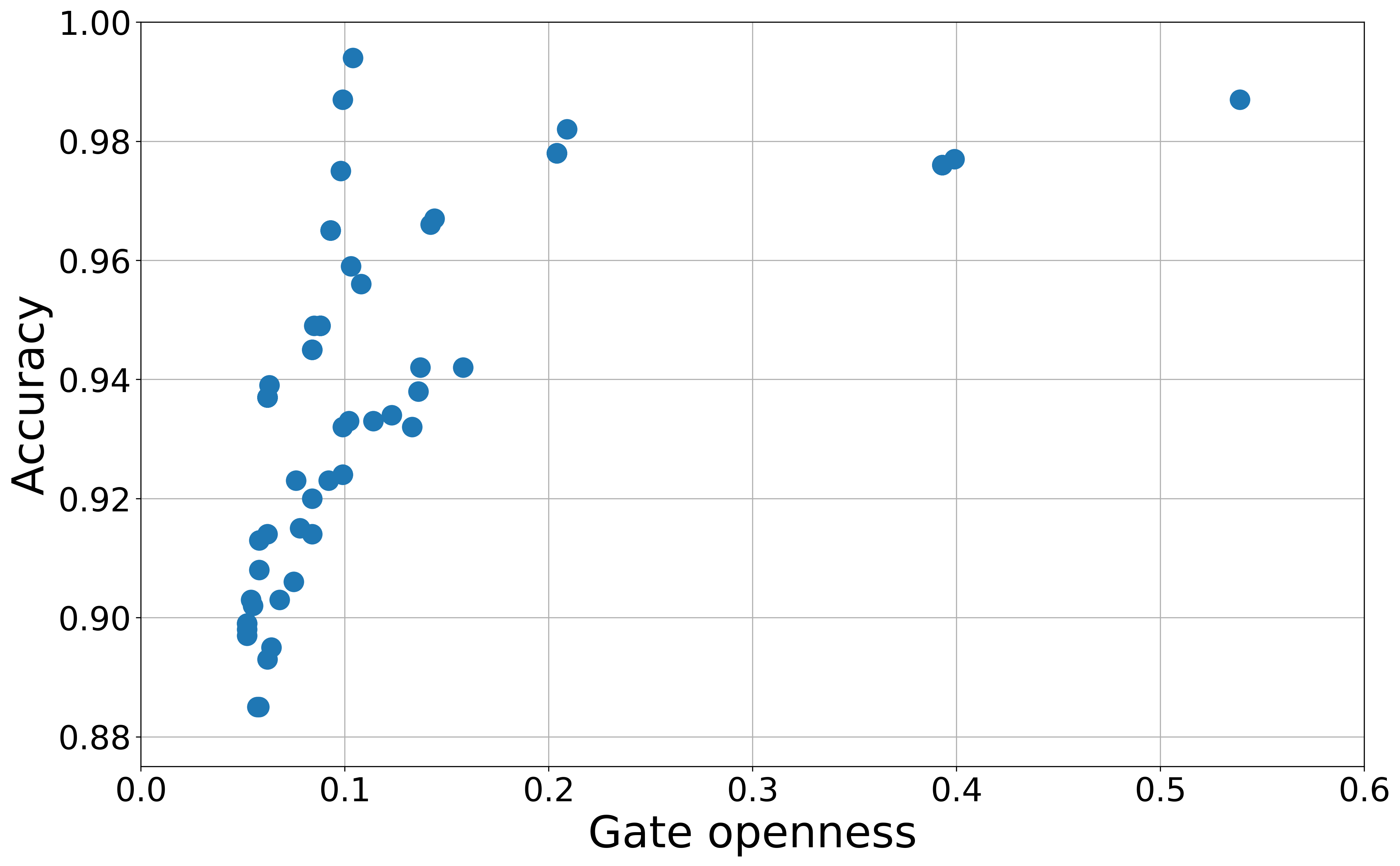
Figure 2: A relationship between accuracy and gate openness for picking task and sequence length $n=100$. The best performance is achieved for gate openness around $10\%$.

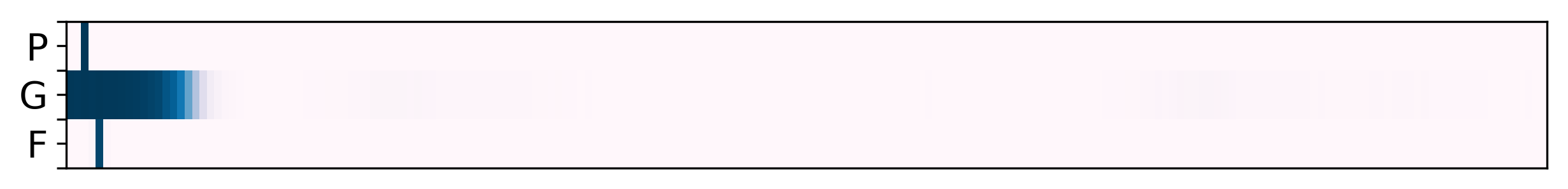
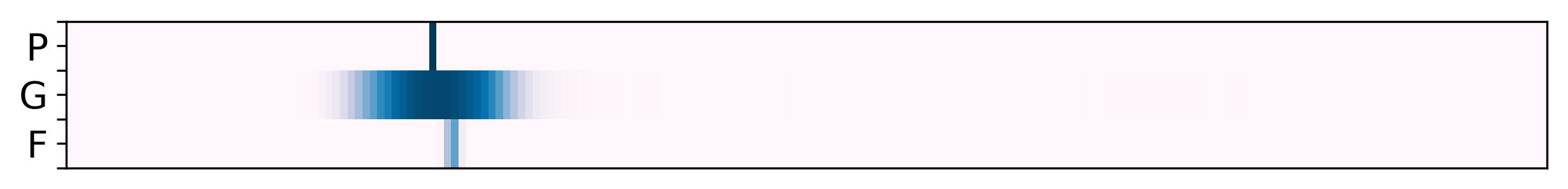
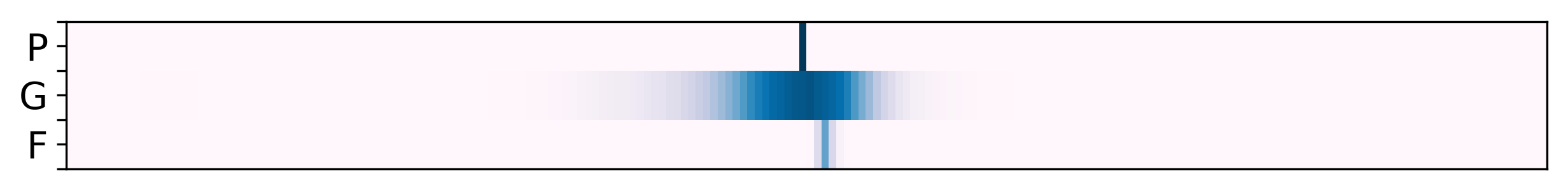
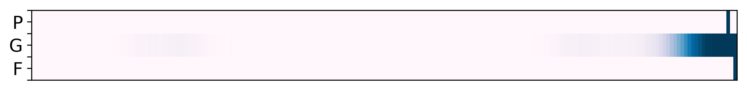
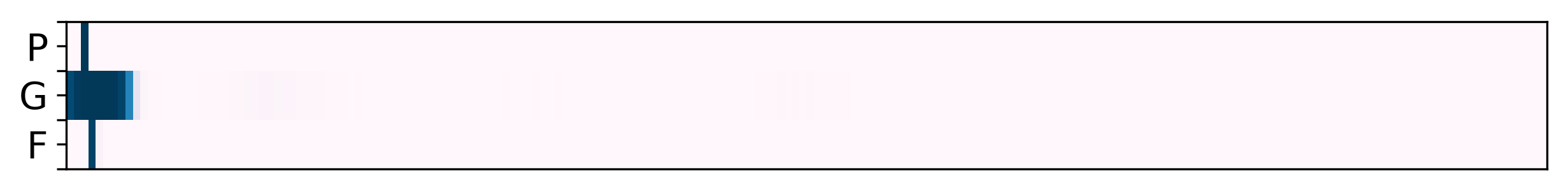
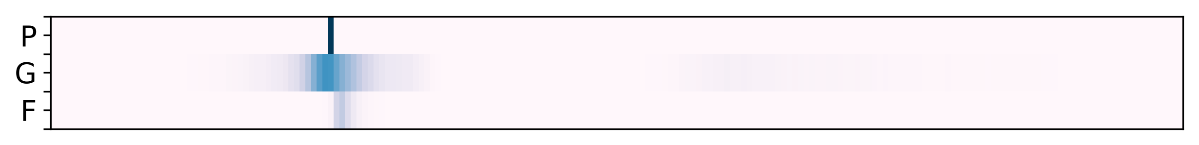
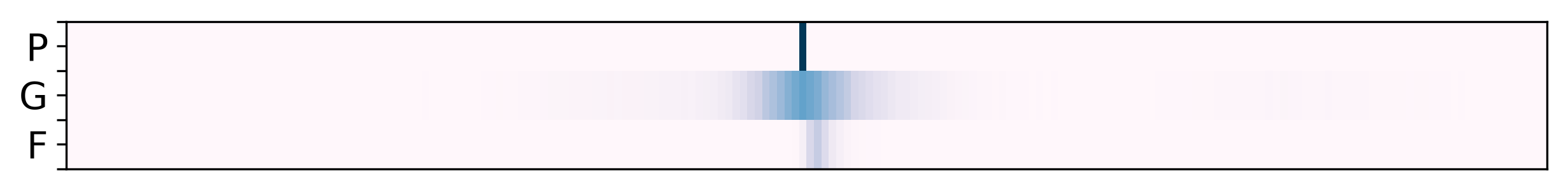
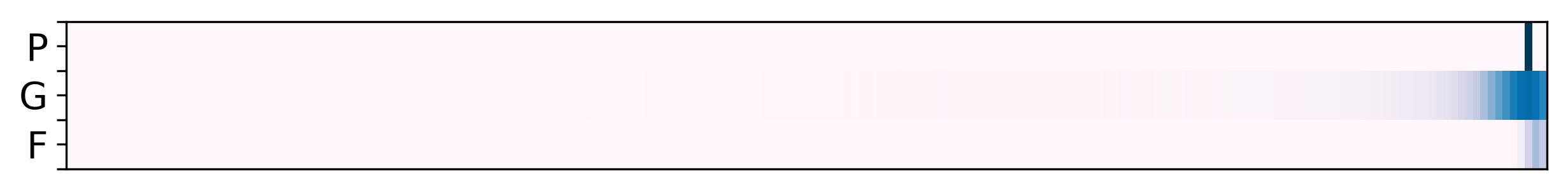
Figure 3: Gate openness (G) conditioned on the position asked (P). Focus (F) is the average of final attention weight set for a given step. Hence, focus sums to one and it is always lower than gate openness (because our model attends only over unique states). Result showed for sequence length $n=200$. The first four plots illustrate FHE model having $99.4\%$ accuracy and $10\%$ gate openness, while the last four are for FHE model having $97\%$ accuracy but $5\%$ gate openness.

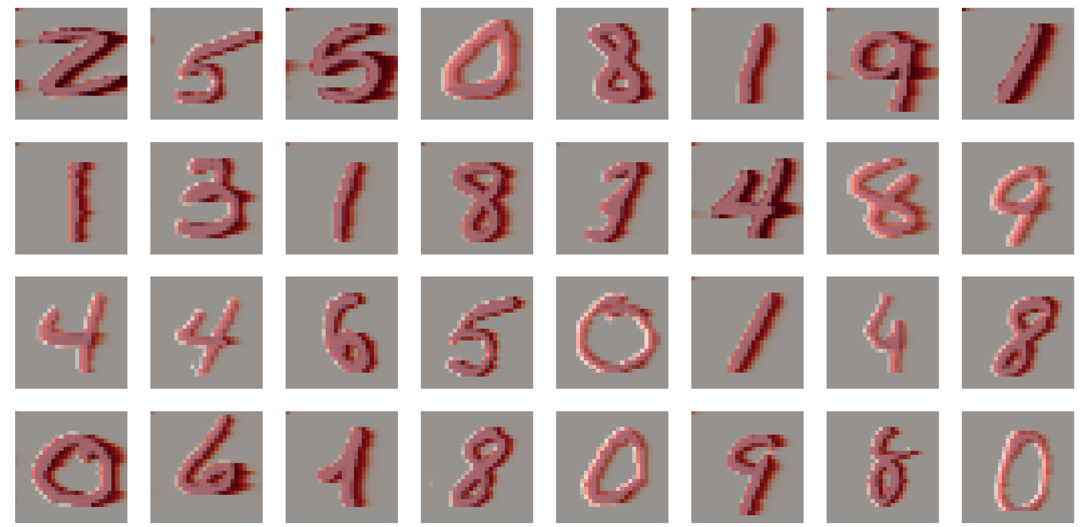
Figure 4: A visualization of the gating mechanism learned using the Pixel-by-Pixel MNIST dataset. Red pixels indicate a gate opening and are overlayed on top of the digit which is white on a gray background. The digits are vectorized row-wise which explains why white pixels appear left of the red pixels.

The picking task is useful to validate our gating mechanism. Once trained we can inspect the positions of the opened gates. Figure 4 shows that our model learns to open gates around $k$’th step only and attend a single gate right after the $k$’th step. The lower-level LSTM is used to count the occurrences of the various digits. That information is then passed to the upper-level LSTM at a single gate. The attention mechanism then uses the information around the same time step to provide the mode (i.e.  solve the task).

We tested the generalization ability of FHE. The models trained on short sequences ($n=200$) were evaluated on longer sequences and $k\leq 200$. The results are in Table 4. The models can not be evaluated for $k$ larger than maximum sequence length used during training because the question embeddings are parts of the models. FHE generalizes better to longer sequences by a wide margin. We believe this is due to the boundary gates being open for only the first k-steps, and the attention mechanism not attending over possibly misleading states.

4.2 Pixel-by-Pixel MNIST QA task

Table 5: Accuracy (%) for validation set of Pixel-by-Pixel MNIST QA task. Our model slightly outperform both LSTM1 and LSTM2.

LSTM1	LSTM2	FHE-fixed
97.3	98.4	99.1

We adapt the Pixel-by-Pixel MNIST classification task (LeCun et al., 1998; Le et al., 2015) to the question and answering setting. The passage encoder reads in MNIST digits one pixel at a time. The question asked is whether the image is a specific digit and the answer is either True or False. The data is balanced such that approximately half of the answers are True and the other half are False.

The LSTM2 reached an accuracy of $98.4\%$ on the validation set, and FHE outperformed the baseline by having an accuracy of $99.1\%$. Figure 4 shows a visualization of the gates for the passage encoder learned by the model. The model learns to open the boundary gate almost always around the digit. We also found that for this particular task, the gates do not depend on the question. We hypothesize that this is because it is much easier for the passage encoder to learn to open the gates when there is a white pixel. In any case, these experiments illustrate how our proposed mechanism modulates gates based on input questions and features in the data.

5 Large Scale Natural Language QA Tasks

Next, we explore the more complex task of natural language question answering. We study our approach using the MS MARCO and SearchQA datasets and tasks. These tasks are well-suited for our model since they both involve searching over a long input passage for answers to a question. Our results are that for the MS MARCO task, we achieved scores higher than the baseline models. Our model on SearchQA significantly outperforms very recent work (Buck et al., 2018). We also run ablation studies on the model for MS MARCO task to show the importance of each component in the model.

To obtain competitive results on these difficult question-answering tasks we embed FHE with a modified version of both the question encoder and the answer decoder. All changes with respect to what was presented earlier are detailed in the following sections.

5.1 Question Encoder

Following recent work (Cui et al., 2016; Chen et al., 2017), we use a bidirectional LSTM that first reads the question and then performs self-attention to construct a vector representation of it. At the model-level, the question-encoder module outputs the vector $\mathbf{q}$, which is then used as conditioning information in a FHE.

5.2 Decoder

The answer decoder follows the standard decoding procedure in RNN with attention (Bahdanau et al., 2015; Gulcehre et al., 2016). The only difference is that the decoder looks over the upper-level hidden states $h^{u}_{t}$ learned using a FHE conditioned on the question. The upper-level states $H^{u}$ provide an abstracted, dynamic representation of the passage. Because they receive lower-layer input only when the boundary gate is open, the resulting hidden states can be viewed as a sectional summary of the tokens between these “open” time-steps. The upper layer thus summarizes a passage in a smaller number of states. This can be beneficial because it enables the encoder LSTM to maintain information over a longer time-horizon, reduces the number of hidden states, and makes learning the subsequent attention softmax layer easier.

Pointer Softmax

In order to predict the next answer word and to avoid large-vocabulary issues, we use the pointer softmax (Gulcehre et al., 2016). This method decomposes as two softmaxes: one places a distribution over a shortlist of words and the other places a distribution over words in the document. The softmax parameters are $W_{o}\in R^{|V|\times D_{h}}$ and $b_{o}\in R|V|$, where $|V|$ is the size of the shortlist vocabulary. A switching network enables the model to learn the mixture proportions over the two distributions. Switching variable $z_{j}$ determines how to interpolate between the indices in the document and the shortlist words. It is computed via an MLP. Let $o_{j}$ be the distribution of word in the shortlist, and $\alpha_{j}$ be the distribution over words in the document index. Then the pointer softmax $P_{j}\in R^{|V|+D}$ is $P_{j}=[z_{j}o_{j};(1-z_{j})\alpha_{j}]$.

Table 6: SearchQA results measured in F1 and Exact Match (EM) for validation and test set. Our model and AMANDA  (Kundu & Ng, 2018) are on par with performing while the other models are behind.

Models	Validation		Test
	F1	EM	F1	EM
TF-IDF Max (Dunn et al., 2017)	-	13.0	-	12.7
ASR  (Dunn et al., 2017)	24.1	43.9	22.8	41.3
AQA  (Buck et al., 2018)	47.7	40.5	45.6	38.7
Human  (Dunn et al., 2017)	-	-	43.9	-
LSTM1 + pointer softmax	52.8	41.9	48.7	39.7
LSTM2 + pointer softmax	55.3	44.7	51.9	41.7
Our Model	56.7	49.6	53.4	46.8
Concurrent work
AMANDA  (Kundu & Ng, 2018)	57.7	48.6	56.6	46.8

Table 7: MS MARCO results using BLEU-1 and Rouge-L evaluation. Our model clearly outperforms both standard memory networks and sequence-to-sequence models. In addition in both Bleu-1 and Rouge-L, we outperform strong baselines. Available results for the first three methods are taken from their respective papers (hence the not available ones). Ablation study results show that our model benefits the most from elementwise product between questions and context. The pointer softmax also gives a significant gain for performance.

Generative Models	Validation		Test
	Bleu-1	Rouge-L	Bleu-1	Rouge-L
Seq-to-Seq (Nguyen et al., 2016)	-	8.9	-	-
Memory Network (Nguyen et al., 2016)	-	11.9	-	-
Attention Model (Higgins & Nho, 2017)	9.3	12.8	-	-
LSTM1 + pointer softmax	24.8	26.5	28	28
LSTM2 + pointer softmax	24.3	23.3	27	28
Our Model	27.3	26.7	30	30
Ablation study
Our Model – dot-product between question and context	18.5	19.3	-	-
Our Model – pointer softmax	20.5	18.7	-	-
Our Model – learned boundaries	23.5	24	-	-

Hyper-parameters

All components of the model (FHE, question encoder, decoder) in all natural language QA experiments uses 300 hidden units. FHE hyper-parameters were fixed ($\alpha=0.001$, $\beta=0.5$, $\gamma=50\%$). We use the Adam optimizer (Kingma & Welling, 2014) with a learning rate of 0.001.

5.3 SearchQA Question and Answering Task

Search QA (Dunn et al., 2017) is large scale QA dataset in the form of Question-Context-Answer. The question-answer pairs are real Jeopardy! questions crawled from J!Archive. The contexts are text snippets retrieved by Google. It contains $140,461$ question-context-answer pairs. Each pair is coupled with a set of $49.6\pm 2.10$ snippets, and each snippet is $37.3\pm 11.7$ tokens long on average. Answers are on average $1.47\pm 0.58$ tokens long.

We use the same metric as reported in Buck et al. (2018), which are F1 scores for multi-word answers and Exact Match (EM) for single word answers.

QA Results

Our model outperformed the recently proposed AQA model (Buck et al., 2018) by 8 points in EM and more than 6 points in terms of F1 scores. See detailed results in Table 7.

5.4 MS MARCO Question and Answering Task

The Microsoft Machine Reading Comprehension Dataset (MS MARCO) (Nguyen et al., 2016) is one of the largest publicly available QA datasets. Each example in the dataset consists of a query, several context passages retrieved by the Bing search engine (ten per query on average), and several human generated answers (synthesized from the given contexts).

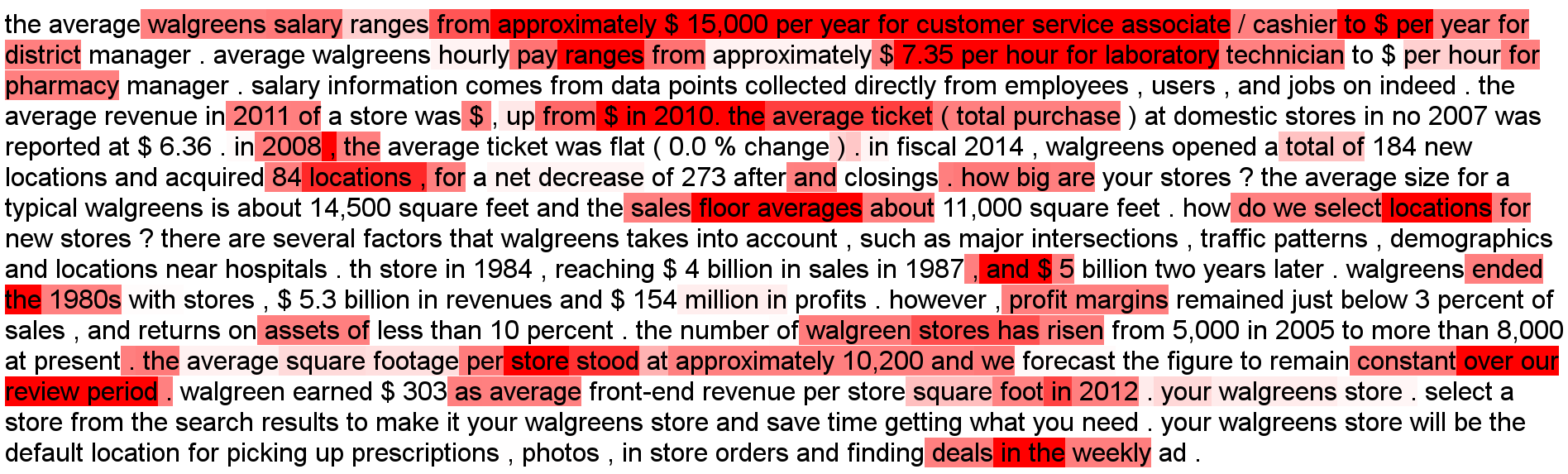
Figure 5: We visualize the attention heat map of the passage encoder using an example from the MS MARCO validation set. Darker background color indicates higher attention (figure better seen on-screen). The question related to this passage is “walgreens store sales average” and the ground truth answer is “Approximately $15,000 per year.”. Our model learns to attend to the passage containing the answer (first line). In addition, most of the other high-intensity passages are related to the question.

Span-based vs Generative

Most of the recent question and answering models for MS MARCO are span-based (Weissenborn et al., 2017; Tan et al., 2017; Shen et al., 2017; Wang & Jiang, 2016). Span-based models are currently state of the art according to Bleu-1 and Rouge scores on the MS MARCO leaderboard, but are clearly limited as they cannot answer questions where the answer is not contained in the passage. In comparison, generative models, such as ours synthesize a novel answer for the given question. Generative models could learn a disentangled representation, and therefore generalize better. Our approach takes the first step towards closing the gap between generative models and span-based models.

We report the model performance using Bleu-1 and Rouge-L, which are the standard evaluation for MS MARCO task.

QA Results

Table 7 reports performance evaluated using the MS MARCO dataset. Specifically, we evaluate the quality of the generated answers for different models. Our model outperforms all competing methods in terms of test set Bleu-1 and Rouge-L.

Ablation Studies

Table 7 shows also the results of learning our model without some of its key components. The ablation studies are evaluated on the validation set only.

The largest gain came from the elementwise-product between question and context. This result is to be expected, since it is difficult for the model to encode the appropriate information without direct knowledge of the question.

The pointer softmax is another important module of the model. The MS MARCO dataset contains many rare words, with around $90\%$ of words appealing less than 20 times in the dataset. It is difficult for the model to generate words it has only seen a few times, and therefore the pointer-softmax provides a significant gain.

Our experiments also show the importance of learned boundaries. This results is supportive of our hypothesis that learned boundaries help with better document encoding, and therefore generates better answers.

Overall, the different components in our model are all needed to achieve the final score.

Model Exploration

Figure 5 reports the results of our attention mechanism on an example from the MS MARCO dataset. Our attention focuses on the relevant passage (the one that contains the answer) as well as other salient phrases of the passage given the question.

Human Evaluation

We performed a human evaluation study to compare answers generated by our model to answers generated by the LSTM1 baseline model in Table 7. We randomly selected 23 test-set questions and their corresponding answers. The order of the questions are randomized for each questionnaire. We collected a total of 690 responses (30 volunteers each given 23 examples) where volunteers were shown both answers side-by-side and were asked to pick their preferred answers. $63\%$ of the time, volunteers preferred the answers generated from our model. Volunteers are students from our lab, and were not aware of which samples came from which model.

6 Conclusion

We introduced a focusing mechanism for encoder recurrent neural networks and evaluated our approach on the popular task of natural-language question answering. Our proposed model uses a discrete stochastic gating function that conditions on a vector representation of the question to control information flow from a word-level representation to a concept-level representation of the document. We trained the gates with policy gradient techniques. Using synthetic tasks we showed that the mechanism correctly learns when to open the gates given the context (question) and the input (passage). Further, experiments on MS MARCO and SearchQA – recent large-scale QA datasets – showed that our proposed model outperforms strong baselines and in the case of SearchQA outperforms prior work.

References

- Andrychowicz & Kurach (2016) Andrychowicz, M. and Kurach, K. Learning efficient algorithms with hierarchical attentive memory. arXiv preprint arXiv:1602.03218, 2016.
- Bahdanau et al. (2015) Bahdanau, D., Cho, K., and Bengio, Y. Neural machine translation by jointly learning to align and translate. International Conference on Learning Representations (ICLR), 2015.
- Bahdanau et al. (2016) Bahdanau, D., Chorowski, J., Serdyuk, D., Brakel, P., and Bengio, Y. End-to-end attention-based large vocabulary speech recognition. In Acoustics, Speech and Signal Processing (ICASSP), 2016 IEEE International Conference on, pp. 4945–4949. IEEE, 2016.
- Bengio et al. (1994) Bengio, Y., Simard, P., and Frasconi, P. Learning long-term dependencies with gradient descent is difficult. Trans. Neural Networks, 5(2):157–166, March 1994. ISSN 1045-9227.
- Buck et al. (2018) Buck, C., Bulian, J., Ciaramita, M., Gajewski, W., Gesmundo, A., Houlsby, N., and Wang., W. Ask the right questions: Active question reformulation with reinforcement learning. In International Conference on Learning Representations, 2018. URL https://openreview.net/forum?id=S1CChZ-CZ.
- Campos et al. (2017) Campos, V., Jou, B., Giró-i Nieto, X., Torres, J., and Chang, S.-F. Skip rnn: Learning to skip state updates in recurrent neural networks. arXiv preprint arXiv:1708.06834, 2017.
- Chan et al. (2016) Chan, W., Jaitly, N., Le, Q., and Vinyals, O. Listen, attend and spell: A neural network for large vocabulary conversational speech recognition. In Acoustics, Speech and Signal Processing (ICASSP), 2016 IEEE International Conference on, pp. 4960–4964. IEEE, 2016.
- Chen et al. (2017) Chen, D., Fisch, A., Weston, J., and Bordes, A. Reading wikipedia to answer open-domain questions. arXiv preprint arXiv:1704.00051, 2017.
- Chung et al. (2016) Chung, J., Ahn, S., and Bengio, Y. Hierarchical multiscale recurrent neural networks. arXiv preprint arXiv:1609.01704, 2016.
- Cui et al. (2016) Cui, Y., Chen, Z., Wei, S., Wang, S., Liu, T., and Hu, G. Attention-over-attention neural networks for reading comprehension. arXiv preprint arXiv:1607.04423, 2016.
- Dunn et al. (2017) Dunn, M., Sagun, L., Higgins, M., Guney, U., Cirik, V., and Cho, K. Searchqa: A new q&a dataset augmented with context from a search engine. arXiv preprint arXiv:1704.05179, 2017.
- El Hihi & Bengio (1995) El Hihi, S. and Bengio, Y. Hierarchical recurrent neural networks for long-term dependencies. In Proceedings of the 8th International Conference on Neural Information Processing Systems, pp. 493–499. MIT Press, 1995.
- Graves (2016) Graves, A. Adaptive computation time for recurrent neural networks. arXiv preprint arXiv:1603.08983, 2016.
- Graves et al. (2014) Graves, A., Wayne, G., and Danihelka, I. Neural turing machines. arXiv preprint arXiv:1410.5401, 2014.
- Gulcehre et al. (2016) Gulcehre, C., Ahn, S., Nallapati, R., Zhou, B., and Bengio, Y. Pointing the unknown words. arXiv preprint arXiv:1603.08148, 2016.
- Higgins & Nho (2017) Higgins, B. and Nho, E. LSTM encoder-decoder architecture with attention mechanism for machine comprehension. 2017.
- Hochreiter (1991) Hochreiter, S. Untersuchungen zu dynamischen neuronalen Netzen. Diploma thesis, Institut für Informatik, Lehrstuhl Prof. Brauer, Technische Universität München, 1991.
- Hochreiter (1998) Hochreiter, S. The vanishing gradient problem during learning recurrent neural nets and problem solutions. Int. J. Uncertain. Fuzziness Knowl.-Based Syst., 6(2):107–116, April 1998. ISSN 0218-4885. doi: 10.1142/S0218488598000094. URL http://dx.doi.org/10.1142/S0218488598000094.
- Kadlec et al. (2016) Kadlec, R., Schmid, M., Bajgar, O., and Kleindienst, J. Text understanding with the attention sum reader network. In Proceedings of the 54th Annual Meeting of the Association for Computational Linguistics, ACL 2016, August 7-12, 2016, Berlin, Germany, Volume 1: Long Papers, 2016.
- Kingma & Ba (2014) Kingma, D. P. and Ba, J. Adam: A method for stochastic optimization. In International Conference on Learning Representations (ICLR), 2014.
- Kingma & Welling (2014) Kingma, D. P. and Welling, M. Auto-encoding variational bayes. In International Conference on Learning Representations (ICLR), 2014.
- Koutnik et al. (2014) Koutnik, J., Greff, K., Gomez, F., and Schmidhuber, J. A clockwork rnn. In Proceedings of The 31st International Conference on Machine Learning, pp. 1863–1871, 2014.
- Kumar et al. (2016) Kumar, A., Irsoy, O., Ondruska, P., Iyyer, M., Bradbury, J., Gulrajani, I., Zhong, V., Paulus, R., and Socher, R. Ask me anything: Dynamic memory networks for natural language processing. In International Conference on Machine Learning, pp. 1378–1387, 2016.
- Kundu & Ng (2018) Kundu, S. and Ng, H. T. A question-focused multi-factor attention network for question answering. arXiv preprint arXiv:1801.08290, 2018.
- Le et al. (2015) Le, Q. V., Jaitly, N., and Hinton, G. E. A simple way to initialize recurrent networks of rectified linear units. CoRR, abs/1504.00941, 2015. URL http://arxiv.org/abs/1504.00941.
- LeCun et al. (1998) LeCun, Y., Bottou, L., Bengio, Y., and Haffner, P. Gradient-based learning applied to document recognition. Proceedings of the IEEE, 86(11):2278–2324, 1998.
- Lu et al. (2017) Lu, J., Xiong, C., Parikh, D., and Socher, R. Knowing when to look: Adaptive attention via a visual sentinel for image captioning. In Proceedings of the IEEE Conference on Computer Vision and Pattern Recognition (CVPR), volume 6, 2017.
- Miller et al. (2016) Miller, A., Fisch, A., Dodge, J., Karimi, A.-H., Bordes, A., and Weston, J. Key-value memory networks for directly reading documents. arXiv preprint arXiv:1606.03126, 2016.
- Nallapati et al. (2016) Nallapati, R., Zhou, B., dos Santos, C. N., Gülçehre, Ç., and Xiang, B. Abstractive text summarization using sequence-to-sequence rnns and beyond. In Proceedings of the 20th SIGNLL Conference on Computational Natural Language Learning, CoNLL 2016, Berlin, Germany, August 11-12, 2016, pp. 280–290, 2016.
- Nguyen et al. (2016) Nguyen, T., Rosenberg, M., Song, X., Gao, J., Tiwary, S., Majumder, R., and Deng, L. Ms marco: A human generated machine reading comprehension dataset. arXiv preprint arXiv:1611.09268, 2016.
- Shen et al. (2017) Shen, Y., Huang, P.-S., Gao, J., and Chen, W. Reasonet: Learning to stop reading in machine comprehension. In Proceedings of the 23rd ACM SIGKDD International Conference on Knowledge Discovery and Data Mining, pp. 1047–1055. ACM, 2017.
- Sordoni et al. (2015) Sordoni, A., Bengio, Y., Vahabi, H., Lioma, C., Grue Simonsen, J., and Nie, J.-Y. A hierarchical recurrent encoder-decoder for generative context-aware query suggestion. In Proceedings of the 24th ACM International on Conference on Information and Knowledge Management, pp. 553–562. ACM, 2015.
- Srivastava et al. (2015) Srivastava, R. K., Greff, K., and Schmidhuber, J. Highway networks. arXiv preprint arXiv:1505.00387, 2015.
- Tan et al. (2017) Tan, C., Wei, F., Yang, N., Lv, W., and Zhou, M. S-net: From answer extraction to answer generation for machine reading comprehension. arXiv preprint arXiv:1706.04815, 2017.
- Wang & Jiang (2016) Wang, S. and Jiang, J. Machine comprehension using match-lstm and answer pointer. arXiv preprint arXiv:1608.07905, 2016.
- Weissenborn et al. (2017) Weissenborn, D., Wiese, G., and Seiffe, L. Making neural qa as simple as possible but not simpler. In Proceedings of the 21st Conference on Computational Natural Language Learning (CoNLL 2017), pp. 271–280, 2017.
- Williams (1992) Williams, R. J. Simple statistical gradient-following algorithms for connectionist reinforcement learning. Machine learning, 8(3-4):229–256, 1992.
- Yang et al. (2016) Yang, Z., Yang, D., Dyer, C., He, X., Smola, A., and Hovy, E. Hierarchical attention networks for document classification. In Proceedings of NAACL-HLT, pp. 1480–1489, 2016.
- Yao et al. (2015) Yao, K., Cohn, T., Vylomova, K., Duh, K., and Dyer, C. Depth-gated recurrent neural networks. arXiv preprint, 2015.
- Yao et al. (2016) Yao, T., Pan, Y., Li, Y., Qiu, Z., and Mei, T. Boosting image captioning with attributes. OpenReview, 2(5):8, 2016.