MSplit LBI: Realizing Feature Selection and Dense Estimation Simultaneously in Few-shot and Zero-shot Learning

Abstract

It is one typical and general topic of learning a good embedding model to efficiently learn the representation coefficients between two spaces/subspaces. To solve this task, $L_{1}$ regularization is widely used for the pursuit of feature selection and avoiding overfitting, and yet the sparse estimation of features in $L_{1}$ regularization may cause the underfitting of training data. $L_{2}$ regularization is also frequently used, but it is a biased estimator. In this paper, we propose the idea that the features consist of three orthogonal parts, namely sparse strong signals, dense weak signals and random noise, in which both strong and weak signals contribute to the fitting of data. To facilitate such novel decomposition, MSplit LBI is for the first time proposed to realize feature selection and dense estimation simultaneously. We provide theoretical and simulational verification that our method exceeds $L_{1}$ and $L_{2}$ regularization, and extensive experimental results show that our method achieves state-of-the-art performance in the few-shot and zero-shot learning.

1 Introduction

This paper discusses the problem of learning representation coefficients between two spaces/subspaces. This is one typical and general research topic that can be used in various tasks, such as learning feature embedding in Few-shot learning (FSL) and capturing relational structures in Zero-Shot Learning (ZSL) (Palatucci et al. [34]). In particular, FSL (Fei-Fei et al. [11]) aims to learn new concepts with only few training samples, while ZSL tends to learn new concepts without any training samples. The semantic spaces such as attributes Lampert et al. [28], textual descriptions Ba et al. [3] and word vectors Fu and Sigal [14] are served as the auxiliary knowledge to assist the ZSL. This paper concerns the FSL and ZSL in transfer learning scenario. The data in the source domain is abundant to train the feature extractors (e.g., deep Convolutional Neural Networks (CNNs) Krizhevsky et al. [26]; Simonyan and Zisserman [38]; Szegedy et al. [41]; He et al. [18]); and the data in the target are very limited to learn/fine-tune a deep model.

The natural solutions of FSL and ZSL are to learn the linear embedding models, which can map the image features to the label space (FSL) (or semantic space (ZSL)). To efficiently learn such a linear model, $L_{1}$ or $L_{2}$ penalty terms are frequently applied to regularize the weights of embedding models. In particular, the $L_{1}$ regularization can capture the strong and sparse signals in the embedding weights, which is also a process of feature selection. Nevertheless, the feature selection property of $L_{1}$ penalty suffers from two problems. 1) the inaccurate estimation of strong signals if irrepresentable condition does not hold Zhao and Yu [55]; 2) the underfitting of training data due to the ignorance of weak signals from the embedding / relational weights. In contrast, $L_{2}$ penalty yet does a proportional shrinkage of feature dimension, and thus it may introduce the bias in learning the embedding model. However, in real-world applications, it is of equal importance to do both the feature selection and well data-fitting. For example, in Text Classification (Forman [13]), Bioinformatics (Saeys et al. [36]) and Neuroimaging Analysis (Sun et al. [40]), researchers need to fit the training data well; and meantime, select a few strong signals (features) which are comprehensible for human beings.

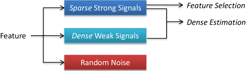
Figure 1: MSplit LBI is learned in linear embedding to decompose the features into sparse strong signals, dense weak signals and random noise. The sparse strong signals facilitate the feature selection. The dense estimation can be done via the sparse strong signals and dense weak signals.

In this paper, we propose that the embedding features consist of random noise, sparse strong signals and dense weak signals. In Sec. 3.2, the MSplit LBI is for the first time proposed to facilitate the decomposition of features. Particularly, in our linear embedding models, the MSplit LBI will decompose the embedding weights into three orthogonal parts (in Sec.3.3), namely, random noise, sparse strong signals and dense weak signals as illustrated in Fig. 1. The sparse strong signals can serve the purpose of feature selection, and the dense estimation can be done by integrating both sparse strong signals and dense weak signals. Furthermore, we theoretically analyze the property of MSplit LBI estimator in Sec. 3.4 which is less biased than $L_{2}-$regularization and can facilitate the feature selection at the same time. We further show the way of using proposed MSplit LBI in FSL and ZSL tasks in Sec. 3.5. Extensive experiments had been done to validate the proposed MSplit LBI can learn better embedding models.

Contribution. The main contributions are several folds: (1) We for the first time propose the idea of decomposing the feature representation into three orthogonal elements, i.e., strong signals, weak signals and random noise. (2) The MSplit LBI algorithm is for the first time proposed to facilitate such orthogonal decomposition and thus learn two estimators: the sparse estimator learning strong signals and the dense estimator additionally capturing the weak signals that also contribute to the estimation. (3) The theoretical analysis is given in terms of the advantages over commonly applied regularization penalties (e.g., $L_{1}$, $L_{2}$ or elastic net); (4) The benefits and effectiveness of proposed methodology are demonstrated on simulation experiments and tasks of feature embedding learning in FSL and relational structure learning in ZSL.

2 Related Work

2.1 Feature Selection and Variable Split

Feature Selection. The advantages of feature selection can be many folds, such as avoid overfitting, or mining the correlations between features and responses, or reducing the time complexity of inference. Existing supervised feature selection methods can be classified into filter methods Yu and Liu [51], wrapper methods Kabir et al. [21] and embedded methods Saeys et al. [36] integrating the feature selection with the classification model. Compared to filter methods, embedded methods have the superiority that they integrate well with classifiers. Furthermore, embedded methods are more computationally efficient than wrapper methods. Therefore, embedded methods, e.g. $L_{0}$ and $L_{1}$ regularization, are widely used in many real-world applications; for instance, object recognition Kavukcuoglu et al. [22], face recognition Wright et al. [47], image restoration Mairal et al. [32], subspace clustering Elhamifar and Vidal [9], few-shot learning Lee et al. [30] and zero-shot learning Kodirov et al. [25]. Because the optimization with $L_{0}$ regularization is NP hard, $L_{1}$ regularization, which is the tightest convex relaxation of $L_{0}$, is used for the sparsity in the most practice.

Variable Split. To deal with $L_{1}$ penalty and other constrains, the operator splitting ideas are adopted by introducing an augmented variable satisfying the sparsity (or non-negative) constraints, such as ADMM Wahlberg et al. [44]; Boyd et al. [5]. By adopting such schemes, the two estimators are introduced and split apart with one being dense and the augmented one pursuing sparsity requirements. For example in Ye and Xie [50]; Huang et al. [20], the variable splitting scheme is proposed to avoid dealing with structural sparsity (such as fused lasso or total variation penalty) directly. In addition to the computational advantage, the Sun et al. [40] discussed another benefit of variable splitting term that by relaxing the distance between two estimators, the dense estimator can show a better prediction power than the sparse one since degree of freedom to capture extra features that can fit data better. To achieve similar effect, one can also use ridge or elastic net models Zou and Hastie [57] to select more correlated features by enforcing strictly convexity via $L_{2}$ penalty.

2.2 Few-shot and Zero-shot Learning

Few-shot Learning. The naive way to implement few-shot learning is fine-tuning the model (trained on the source domain) on the target domain. However, the model will easily overfit the several training samples and hardly generalize to testing samples. The $k$-nearest neighbor classifier is often used as the baseline in few-shot learning Koch et al. [23]; Santoro et al. [37]. When only one sample per target class is provided in training, i.e. $k=1$, it can be viewed as a linear model. The Siamese neural network is proposed by Koch et al. [23], which contains twin deep feature extractors for two input images. The $L_{1}$ component-wise distance between two feature vectors are computed with the sigmoid activation function. Snell et al. [39] propose the prototypical network which is combined by the deep feature extractor and linear model. Testing images are mapped into the learned embedding space, then classified based on a softmax over distances to class prototypes.

Zero-shot Learning. Currently, most popular methods in ZSL are linear models, as deep models may easily overfit on target domain Zhang et al. [52]. $L_{1}$ and $L_{2}$ regularization terms are frequently used in these linear models. Palatucci et al. [34]; Li et al. [31] try to learn the linear mapping from the image feature space to semantic embedding space. $L_{2}$ regularization is utilized to avoid overfitting. Li et al. [31] considers ZSL as a sparse coding problem. They try to regress the image features use the learned dictionary with sparse codes (semantic embeddings). $L_{1}$ regularization is utilized to realize sparsity. In Wang et al. [46]; Zhao et al. [54], structural knowledge is learned by linearly regressing unseen semantic embeddings on seen ones. $L_{1}$ regularization is introduced, because they assume the connection between seen and unseen classes is sparse.

3 Methodology

We take the transfer learning setting. The source domain and target domain data are denoted as $\{(\mathbf{x}_{1}^{s},{y}_{1}^{s}),...,(\mathbf{x}_{N^{s}}^{s},{y}_{N^{s}}^{s})\}$ and $\{(\mathbf{x}_{1}^{t},{y}_{1}^{t}),...,(\mathbf{x}_{N^{t}}^{t},{y}_{N^{t}}^{t})\}$ respectively. Here $\mathbf{x}_{i}^{s}\in\Re^{d}$ and $\mathbf{x}_{i}^{t}\in\Re^{d}$ indicate the visual features; and ${y}_{k}^{s}\in\mathbf{Y}^{s}$ and ${y}_{k}^{t}\in\mathbf{Y}^{t}$ are the class labels. We concern two different settings. (1) Few-shot setting. Only few labeled training images are available in the target domain. (2) Zero-shot setting. No training data but auxiliary knowledge is available in target domain.

Each class is embedded in the label space and expressed as $\mathbf{e}_{k}^{s}$ and $\mathbf{e}_{k}^{t}$ $\in\Re^{p}$. The label embedding of each class is a one-hot vector in FSL, while we use auxiliary knowledge Lampert et al. [28]; Fu et al. [16] to embed each label to be a semantic vector in ZSL. Thus we can learn the linear classification models on training data. Without loss of generality, we first consider the linear regression of the label embeddings $\mathbf{E}=\{\mathbf{e}_{1},...,\mathbf{e}_{N}\}\in\mathbb{R}^{N\times p}$ using visual features $\mathbf{X}=\{\mathbf{x}_{1},...,\mathbf{x}_{N}\}\in\mathbb{R}^{N\times d}$. It is formulated as

$$\mathbf{E}=\mathbf{X}\mathbf{B},$$ (3.1)

where $\mathbf{B}\in\Re^{d\times p}$ is the linear embedding matrix.

In particular, to learn the mapping, we optimize the following formulation,

$$\bm{B}=\arg\min_{\bm{B}}\>\ell(\bm{B},\mathbf{X})+\lambda\Omega\left(\bm{B}\right)$$ (3.2)

where $\ell(\bm{B},\mathbf{X})=\left\|\mathbf{X}\mathbf{B}-\mathbf{E}\right\|^{2}$ is the loss function over the training samples. $\Omega\left(\bm{B}\right)$ indicates the regularization term over $\mathbf{B}$. The $\lambda$ is the regularization parameter.

3.1 Weakness of Lasso Embedding

Various forms of regularization have been used in previous work such as $L_{2}-$penalty Fu and Sigal [14]; Romera-Paredes and Torr [35] and $L_{1}-$penalty Kodirov et al. [25]; Wang et al. [46]. Here we want to learn sparse weights $\mathbf{B}$ to capture the strong signals in the embedding. One can apply the $L_{1}$ regularization as,

$$\arg\min_{\mathbf{B}}\ell(\mathbf{B},\mathbf{X})+\lambda\sum_{j=1}^{p}\left\|\mathbf{B}_{(j)}\right\|_{1}$$ (3.3)

where $\mathbf{B}_{(j)}$ refers the $j$-th column. Eq (3.3) turns out to be a classical Lasso formulation which can linearly regress the sparse strong signals and set dense weak signals to be zeros. In general, Lasso is sign consistent if there exists a sequence $\lambda_{n}$ such that $P\left(\hat{\mathbf{B}}\left(\lambda_{n}\right)=_{s}\lambda^{*}\right)\rightarrow 1$, as $n\rightarrow\infty$ and if Irrepresentable Condition and Beta Min condition hold (Fan and Li [10]; Wainwright [45]; Zhao and Yu [56]). Here we define $=_{s}$ such that $\hat{\mathbf{B}}\left(\lambda\right)=_{s}\mathbf{B}^{*}$ iff $sgn\left(\hat{\mathbf{B}}\left(\lambda\right)\right)=sgn\left(\mathbf{B}^{*}\right)$ element-wise; and $sgn\left(x\right)=1$ if $x>0$; $=-1$ if $x<0$; $=0$ otherwise. $\mathbf{B}^{*}$ indicate the true sparse embedding weights with the corresponding regularizing parameter $\lambda^{*}$.

The Irrepresentable and Beta Min conditions are not easy to be satisfied in many real-world applications. The Irrepresentable Condition implies the low correlation between the informative and uninformative feature dimensions. Unfortunately, the correlated variables of features, especially in a high-dimensional space ($p>>n$), are a perennial problem for the Lasso. Such a problem will frequently lead to systematic failures and an inaccurate estimation of index set of strong signals. On the other hands, The Beta Min condition requires the strong feature dimension of non-zero coefficients should be higher than the threshold pre-specified. Nevertheless, some feature dimensions of weak signals that are totally ignored by Lasso, may still be very helpful in estimating the response variables in Eq (3.3); and thus the inferior linear embedding mapping is usually learned than the embedding learned by ridge regression. For example, the recent neuroimaging analysis work Sun et al. [40] showed the lesion features (strong signals) are most contributed to identifying the disease concerned. In addition, although “procedural bias" features are weak signals, they can still be leveraged to improve the prediction of the disease.

3.2 Multiple Split LBI

This paper targets at alleviating the Irrepresentable Condition and capturing the weak signal in Eq (3.3). The key idea is to generalize the Split LBI algorithm (Huang et al. [20]) to general loss function with response variables embedded in multiple ($p>1$) columns ($\mathbf{E}\in\mathbb{R}^{N_{s}\times p}$). Thus, we call it Multiple Split LBI (MSplit LBI). Specifically, rather than directly dealing with $\sum_{i=1}^{p}\|\mathbf{B}_{(j)}\|_{1}$ in Eq (3.3), we introduce an augmented variable $\mathbf{\Gamma}$ of the same size as $\mathbf{B}$. Here we want $\mathbf{\Gamma}$ to: (1) be enforced sparsity of each column and select the set of strong signals (2) be close to $\mathbf{B}$ from which the distance is controlled by the variable splitting term $\frac{1}{2\nu}\|\mathbf{B}-\mathbf{\Gamma}\|_{F}^{2}$ in the following loss function:

$$\ell(\mathbf{B},\mathbf{\Gamma})=\ell(\mathbf{B},\mathbf{X})+\frac{1}{2\nu}\|\mathbf{B}-\mathbf{\Gamma}\|_{F}^{2} \left(\nu>0\right)$$ (3.4)

To pursue the sparsity requirement of $\mathbf{\Gamma}$, we utilize Linearized Bregman Iteration (LBI) on each column of $\mathbf{B}$ and concatenate them together (please refer supplementary material for details), which can give a sequence of estimation as a regularization solution path, i.e. $\{\mathbf{B}_{k},\mathbf{\Gamma}_{k},\widetilde{\mathbf{B}}_{k}\}$,

$$\mathbf{B}_{k+1} =\mathbf{B}_{k}-\kappa\alpha\nabla_{\mathbf{B}}\ell(\mathbf{B}_{k},\mathbf{\Gamma}_{k}),$$ (3.5a)

$$\mathbf{Z}_{k+1} =\mathbf{Z}_{k}-\alpha\nabla_{\mathbf{\Gamma}}\ell(\mathbf{B}_{k},\mathbf{\Gamma}_{k}),$$ (3.5b)

$$\mathbf{\Gamma}_{k+1} =\kappa\cdot\mathcal{S}\left(\mathbf{Z}_{k+1},1\right),$$ (3.5c)

$$\widetilde{\mathbf{B}}_{k+1} =\mathrm{\mathbf{P}}_{\widetilde{\mathbf{S}}_{k+1}}\mathbf{B}_{k+1}=\mathbf{B}_{k+1}\circ\left[1\{i\in\widetilde{\mathbf{S}}_{(j),k+1}\}\right]_{\{i,j\}}$$ (3.5d)

where $\mathbf{Z}_{0}=\mathbf{\Gamma}_{0}=\widetilde{\mathbf{B}}_{0}=\mathbf{0}\in\mathbb{R}^{d\times p}$, $\widetilde{\mathbf{S}}_{k}=\mathrm{supp}(\mathbf{\Gamma}_{k})$ and

$$\mathcal{S}\left(\mathbf{Z},\lambda\right)=\mathrm{sign}(\mathbf{Z})\cdot\max\left(|\mathbf{Z}|-\lambda,\ 0\right)\ (\lambda\geq 0).$$

By implementing the soft-thresholding $\mathcal{S}\left(\mathbf{Z},1\right)$ in Eq(3.5c), the LBI returns a path of sparse estimators $\mathbf{\Gamma}_{k}$ with different sparsity levels at each iteration. The parameter $t_{k}=k\alpha$ is the regularization parameter which plays a similar role with $\lambda$ in Eq (3.3). In real applications, it can be determined via cross validation (please refer to Osher et al. [33] and therein). The parameter $\kappa$ is the damping factor. The larger value of $\kappa$ can de-bias estimators however at the sacrifice of computational efficiency. Parameter $\alpha$ is the step size, which should satisfy $\kappa\alpha\leq\nu/\kappa(2+\nu\Lambda_{H})$ (Huang et al. [20]) to ensure the statistical property. Parameter $\nu$ in Eq (3.4) controls the distance between $\mathbf{B}$ and $\tilde{\mathbf{B}}$. Such two estimators are tending to be close with smaller value of $\nu$.

3.3 Decomposition property of MSplit LBI

The proposed MSplit LBI has several advantages. Most importantly, it has the decomposition property. Specifically, the path of dense estimators $\mathbf{B}_{k}$ computed by Eq (3.5a–3.5d) has the following orthogonal decomposition of elements,

$$\mathbf{B}_{k}={\mathrm{Signal_{strong}}\oplus\mathrm{Signal_{weak}}\oplus\mathrm{Random\ Noise}}$$ (3.6)

The strong signals are captured by the projection of $\mathbf{B}_{k}$ to the subspace of support set of $\mathbf{\Gamma}_{k}$ (Eq (3.5d)), i.e. $\widetilde{\mathbf{B}}_{k}$. Hence $\mathbf{B}_{k}$ shares the same value of strong signals with $\widetilde{\mathbf{B}}_{k}$. The remainder of such projection is heavily influenced by weak signals, which are captured by non-zero elements of $\mathbf{B}_{k}$ with comparably large magnitude, while others with tiny values are regarded as random noise. Hence, the algorithm gives a path of two estimators: $\mathbf{B}_{k}$ and $\widetilde{\mathbf{B}}_{k}$. Thus, our goal includes two folds: (1) Use $\widetilde{\mathbf{B}}_{k}$ to select the interpretable strong signals; (2) use $\mathbf{B}_{k}$ for prediction since it can additionally leverage weak signals for better fitness of data.

The capture of weak evidences are influenced by parameter $\nu$ and $t_{k}$. Note that with larger value of $\nu$, the $\mathbf{B}$ has more degree of freedom to capture weak signal with less constraint between $\mathbf{B}$ and $\widetilde{\mathbf{B}}$, and vise-versa. Besides, it’s the trade-off between (1) model selection consistency and (2) prediction task. On one hand, the irrepresentable condition is more easier to satisfy with larger value of $\nu$ and On the other hand, it will lower the signal-to-noise ratio and hence deteriorate the estimation of the parameter.

For the regularization parameter $t_{k}$, note that as the algorithm iterates, it tends to give $\widetilde{\mathbf{B}}_{k}$ with less sparsity levels and $\lim_{k\to\infty}\|\widetilde{\mathbf{B}}_{k}-\mathbf{B}_{k}\|_{F}^{2}\to 0$. In such case, the estimation of strong signals are inaccurate and $\mathbf{B}$ has not degree of freedom to capture weak signals.

Compared against Lasso-type penalty, our MSplit LBI generally has more advantages, beside of its simpler iterative scheme: (1) MSplit LBI can capture weak signals which are ignored by $\ell_{1}$ penalty due to the Beta Min condition. (2) According to Theorem 1 in Huang et al. [20], the irrepresentable condition is more easier to be met when $\nu$ is large enough, leading to more robust model selection consistency. (3) Combined with the less bias property of LBI, the estimation of strong signal is more accurate than Lasso as discussed in next subsection.

3.4 Theoretical Analysis of MSplit LBI

Bias Vs. Unbiased. Although the ridge-type penalty and elastic net can weaken the irrepresentable condition by de-correlating column-wise correlation, the regularization parameter will introduce bias during the estimation of strong signals. In contrast, our MSplit LBI is unbiased estimator for strong signals and for weak signals when $\nu\to\infty$. This section introduces two lemmas comparing the differences.

To see this, the following lemma describes the biased estimator given by ridge regression and elastic net under the simplest case. In the following, we use ($\beta$, $\tilde{\beta}$) to denote the vector notation of ($\mathbf{B}$, $\mathbf{\widetilde{B}}$).

Lemma 1.

Assume $y=\beta^{\star}+\varepsilon$ where $\varepsilon$ has independent identically distributed components, each of which has a sub-Gaussian distribution with 0 mean. $\mathbf{S}=\{i:\beta_{i}^{\star}\gtrsim\sqrt{\frac{s\log{p}}{n}}\}$, the ridge estimator and the elastic net estimators

$$\beta_{S}^{ridge} =\arg\min\frac{1}{2}\|y-\beta\|_{2}^{2}+\frac{\lambda_{\ell_{2}}}{2}\|\beta\|_{2}^{2}$$ (3.7)

$$\beta_{S}^{elastic} =\arg\min\frac{1}{2}\|y-\beta\|_{2}^{2}+\frac{\lambda_{\ell_{2}}}{2}\|\beta\|_{2}^{2}+\lambda_{\ell_{1}}\|\beta\|_{1}$$ (3.8)

we have

$$\mathrm{E}(\beta_{\mathbf{S}}^{ridge}) =\frac{1}{1+\lambda_{\ell_{2}}}\beta_{\mathbf{S}}^{\star}$$ (3.9)

$$\mathrm{E}(\beta_{\mathbf{S}}^{elastic}) =\frac{\beta_{\mathbf{S}}^{\star}}{1+\lambda_{\ell_{2}}}+\frac{1}{1+\lambda_{\ell_{2}}}\mathbf{E}_{\varepsilon_{\mathbf{S}}\leq-\beta_{\mathbf{S}}^{\star}-\lambda_{\ell_{1}}}(\varepsilon_{\mathbf{S}}+\lambda_{\ell_{1}})$$

$$\frac{\beta_{\mathbf{S}}^{\star}}{1+\lambda_{\ell_{2}}}P(-\beta_{\mathbf{S}}^{\star}-\lambda_{\ell_{1}}\leq\varepsilon_{\mathbf{S}}\leq-\beta_{\mathbf{S}}^{\star}+\lambda_{\ell_{1}})$$

$$+\frac{1}{1+\lambda_{\ell_{2}}}\mathbf{E}_{\varepsilon_{\mathbf{S}}\geq\lambda_{\ell_{1}}-\beta_{\mathbf{S}}^{\star}}(\varepsilon_{\mathbf{S}}-\lambda_{\ell_{1}})$$ (3.10)

When $\kappa\to\infty$, $\alpha\to 0$, the 3.5a to 3.5c with $\{\mathbf{B},\mathbf{\Gamma}\}$ replaced with $\{\beta,\gamma\}$ converges to

$$0 =-\nabla_{\beta}\ell(\beta_{t},\gamma_{t}),$$ (3.11a)

$$\dot{\rho}_{\gamma_{t}} =-\nabla_{\gamma_{\widetilde{\mathbf{S}}_{t}^{c}}}\ell(\beta_{t},\gamma_{t}),$$ (3.11b)

$$\rho_{\gamma_{t}} \in\partial\|\gamma_{t}\|_{1},$$ (3.11c)

Then the following lemma states that under the case defined in lemma 1, we can give more accurate estimation of $\beta_{S}^{\star}$, and also a slightly biased estimation of $\beta_{T}^{\star}$:

Lemma 2.

Under the same setting defined in lemma 1, if there exists $\bar{t}$ such that $\widetilde{\mathbf{S}}_{t}=\mathbf{S}$, then $\beta_{\bar{t}}$ in 3.11 satisfies

$$\beta_{\mathbf{S},\bar{t}}=\beta_{\mathbf{S}}^{\star}+\varepsilon_{\mathbf{S}},\ \beta_{\mathbf{S}^{c},\bar{t}}=\frac{\nu}{1+\nu}\beta_{\mathbf{S}^{c}}^{\star}+\frac{\nu}{1+\nu}\varepsilon_{\mathbf{S}^{c}}$$ (3.12)

and therefore

$$\mathbf{E}(\beta_{\mathbf{S},\bar{t}})=\beta_{\mathbf{S}}^{\star},\ \mathbf{E}(\beta_{\mathbf{S}^{c},\bar{t}})=\frac{\nu}{1+\nu}\beta_{\mathbf{S}^{c}}^{\star}$$ (3.13)

Hence, for strong signals, when $\nu$ is large enough, not only the model selection consistency is easier to satisfy compared to $\ell_{1}$, but also the estimation of them are bias-free while $\ell_{1},\ell_{2}$ and elastic net are with biases. Moreover, $\beta_{\bar{t}}$ can also capture weak signals in $\mathbf{S}^{c}$ with bias dependent on $\nu$. According to 3.12, larger $\nu$ can give less bias estimation ($\frac{1}{1+\nu}\beta_{\mathbf{S}^{c}}^{\star}$) at the sacrifice of more noise introduced ($\frac{\nu}{1+\nu}\varepsilon_{\mathbf{S}^{c}}$). Note that the lemma 1 and 2 are given under $X=I$ in linear model, the more general cases are left to appendix.

3.5 Learning by Multiple Split LBI

As mentioned in previous sections, the MSplit LBI essentially has the advantage of extracting strong signals and weak signals, which can efficiently learn the embedding in few-shot and zero-shot learning scenarios. In these two tasks, the strong signals correspond to the good sparse embedding, while the weak signals can capture the weak evidences which are also useful to train the embedding.

Few-shot Learning. Our model can be directly used to solve this task. We firstly use the source domain to learn the feature extractor (i.e. deep CNNs). Then, image features from target domain are extracted using the trained CNNs. As few labeled training data in target domain are provided, we use the MSplit LBI, i.e. Eq. (3.4 and 3.5), to learn the linear embedding $\mathbf{B}$ from image features $\mathbf{X}$ to (one-hot) label embeddings $\mathbf{E}$. Here, the label embedding of each training datum is a one-hot vector with 1 on the position corresponding to the label, while the values on other positions are 0. With the learned embedding $\mathbf{B}$, a testing image is first embedded to the label embedding space $\hat{\mathbf{e}}_{i}^{t}=\mathbf{x}_{i}^{t}\mathbf{B}$, then labeled as the one with maximum value $\hat{y}_{i}^{t}=\operatorname*{argmax}_{k}\hat{\mathbf{e}}_{i(k)}^{t}$. The element $\hat{\mathbf{e}}_{i(k)}^{t}$ denotes the $k$th element in the vector $\hat{\mathbf{e}}_{i}^{t}$.

Zero-shot Learning. On this task, our method is based on the structural knowledge transfer. Specifically, the structure among classes is learned in the semantic label embedding space by linearly regressing the label embeddings of target domain classes ($\mathbf{E}^{t}$) on source target domain classes ($\mathbf{E}^{s}$). The Eq. (3.4) is adapted to be $\mathbf{E}^{t}=\mathbf{E}^{s}\mathbf{B}$. Similar as Snell et al. [39] , we use the prototype to represent each class and implement nearest neighbour classification in the image feature space. The prototype of each source domain class is calculate as the mean vector of all samples in the class, i.e. $\mathbf{f}_{k}^{s}=\frac{1}{N^{s}_{k}}\sum_{i}^{N^{s}_{k}}{\mathbf{x}_{i}^{s}}\;\;s.t.\;y_{i}^{s}=k$. ${N^{s}_{k}}$ denotes the number of training samples from the $k$th seen class. Then the learned structure ($\mathbf{B}$) is transferred to the image feature space for synthesizing the prototypes of all target domain classes $\hat{\mathbf{F}}^{t}=\mathbf{F}^{s}\mathbf{B}$, where $\mathbf{F}^{s}=\{\mathbf{f}_{1}^{s},...,\mathbf{f}_{K^{s}}^{s}\}$ and $\hat{\mathbf{F}}^{t}=\{\hat{\mathbf{f}}_{1}^{t},...,\hat{\mathbf{f}}_{K^{t}}^{t}\}$ denote all prototypes in source and target domain respectively. A testing image is classified based on the distance to these synthesized prototypes $\hat{y}_{i}^{t}=\operatorname*{argmin}_{k}{\|\mathbf{x}_{i}^{t}-\hat{\mathbf{f}}_{k}^{t}\|_{F}}$. In the experiments, we will illustrate the learned strong and weak signals in our model.

4 Experiments

In this section, we conduct three parts of experiments. First, the simulation experiments are conducted to statistically validate the advantages of our MSplit LBI over Lasso ($L_{1}-$penalty), Ridge Regression ($L_{2}-$penalty) and Elastic Net. Furthermore, we have the experiments on zero-shot and few-shot learning to illustrate the effectiveness of our model. Finally, some visible evidences about the captured strong and weak signals are shown in the Sec. 4.2.1.

4.1 Simulation Experiments

In this section, we conduct a simulation experiment. We set $N=100$, $p=80$ and generate $X\in\mathbb{R}^{N\times d}$ denoting $N$ $i.i.d$ samples from $\mathcal{N}(0,\Sigma)$ with $\Sigma_{i,j}=1$ for $(i=j)$ and $=\sigma$ for $i\neq j$. We consider four settings in which $\sigma$ increases from 0.2 to 0.8 with space 0.2. Then we generate $y=X\beta^{\star}+\varepsilon$ with $\beta_{i}^{\star}=2$ if $1\leq i\leq 5$; $=0.2$ if $6\leq i\leq 40$; $=0$ otherwise and $\varepsilon\sim\mathcal{N}(0,0.5\cdot I_{N})$.

	$\sigma=0.2$	$\sigma=0.4$
MLE	0.2368 $\pm$ 0.0449	0.2739 $\pm$ 0.0516
Ridge	0.2057 $\pm$ 0.0388	0.2324 $\pm$ 0.0403
Elastic Net	0.1295 $\pm$ 0.0167	0.1359 $\pm$ 0.0178
Lasso	0.1323 $\pm$ 0.0166	0.1418 $\pm$ 0.0187
MSplit LBI ($\tilde{\beta}$)	0.1463 $\pm$ 0.0241	0.1714 $\pm$ 0.0255
MSplit LBI ($\beta$)	0.1238 $\pm$ 0.0112	0.1312 $\pm$ 0.0117
	$\sigma=0.6$	$\sigma=0.8$
MLE	0.3358 $\pm$ 0.0630	0.4751 $\pm$ 0.0891
Ridge	0.2723 $\pm$ 0.0423	0.3479 $\pm$ 0.0455
Elastic Net	0.1643 $\pm$ 0.0241	0.2265 $\pm$ 0.0263
Lasso	0.1777 $\pm$ 0.0279	0.2369 $\pm$ 0.0254
MSplit LBI ($\tilde{\beta}$)	0.2016 $\pm$ 0.0206	0.2421 $\pm$ 0.0159
MSplit LBI ($\beta$)	0.1461 $\pm$ 0.0120	0.1749 $\pm$ 0.0127

Table 1: The estimation error of $\|\hat{\beta}-\beta^{\star}\|_{2}/\|\beta^{\star}\|_{2}$

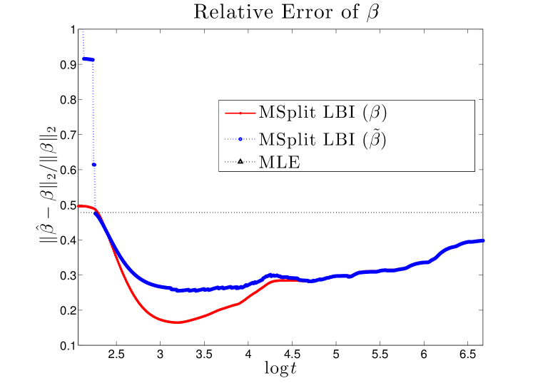
Figure 2: The comparative error of $\{\beta_{k},\tilde{\beta}_{k}\}$ in the regularization solution of MSplit LBI. Red curve represents the $\beta_{k}$ (the dense estimator that can capture both strong and weak evidences); blue curve represents the $\tilde{\beta}_{k}$ (the sparse estimator that captures strong evidences); black dot line represents the estimation of MLE.

We compare Maximum Likelihood Estimator (MLE), Lasso, Ridge, Elastic Net and two estimators, $\beta_{k}$ and $\tilde{\beta}_{k}$ (counterparts of $\mathbf{B}_{k}$ and $\widetilde{\mathbf{B}}_{k}$ in 3.5) in MSplit LBI. For $\lambda$ in Lasso, Ridge and Elastic Net, it ranges from $\{0,0.002\cdot\lfloor\lambda_{\max}/(500-1)\rfloor,0.004\cdot\lfloor\lambda_{\max}/(500-1)\rfloor,...,\lambda_{\max}\}$, which $\lambda_{\max}$ (which we take 5 here) is large enough in our settings to be ensured greater than $\max_{i}\{\frac{X_{i}^{T}y}{N}\}$. For mixture parameter $\alpha$ in Elastic Net, it’s optimized from $\{0,0.05,0.1,...,1\}$. For MSplit LBI, we set $\kappa=5$, $\alpha=\frac{\kappa}{(2+\nu\|X^{\star}X\|_{2})}$. The parameter $\nu$ varies with $\sigma$, it is set to 3 if $\sigma=0.2$, 5 if $\sigma=0.4$ 3, 7 if $\sigma=0.6$ and 10 if $\sigma=0.4$. In each setting ($\sigma$), we simulated 20 times and in each time, we recorded the minimum comparative error of $\beta^{\star}$ optimized from gird of parameters of each method.

As shown in Tab. 1, the $\beta$ of MSplit LBI outperforms others in all cases. Note that $\beta$ is superior than $\tilde{\beta}$ since the former can capture weak evidences. Besides, the advantage over lasso is more obvious when $\sigma$ grows. Particularly, when $\sigma=0.8$, the irrepresentable condition is hard to be satisfied for Lasso while easier for MSplit LBI when $\nu$ is large enough.

The Fig. 2 shows the curve of comparative error of $\{\beta_{k},\tilde{\beta}_{k}\}$ in the regularization solution. From the start when $k=1\thinspace(t_{k}=0)$, $\tilde{\beta}=0$ and $\beta$ is the solution of ridge regression with $\lambda=\frac{1}{2\nu}$. As $t_{k}$ evolves, more strong signals are selected and $\beta_{k}$ is more similar to $\tilde{\beta}_{k}$ in strong evidences. At some point (near 3.2), the $\beta_{k}$ can not only capture strong evidences and also can capture weak evidences to fit data better. When $t_{k}$ continues to grow, the $\|\beta_{k}-\tilde{\beta}_{k}\|_{2}$ gets smaller (blue curve ($\tilde{\beta}_{k}$) and red curve ($\beta_{k}$) converges together).

4.2 Zero-shot Learning

Methods	AwA	CUB	ImageNet
			Top-1	Top-5
DAP/IAP	41.4/42.2	-	–	–
SJE	66.7	50.1	–	–
SC_struct	72.9	54.7	–	–
LatEm	76.1	47.4	–	–
SS-Voc	78.3	-	9.50‡	16.80‡
ConSE	-	-	7.80	15.50
DeViSE	-	-	5.20	12.80
JLSE	80.46	42.11	–	–
MFMR-joint	83.5	53.6	–	–
ESZSL	79.53	51.90	–	–
RKT	81.41	55.59	–	–
Lasso	83.19	56.00	8.30	18.72
Ridge	83.72	51.00	6.47	16.80
MSplit LBI ($\tilde{\beta}$)	84.58	56.62	7.98	17.83
MSplit LBI ($\beta$)	85.34	57.52	8.35	18.76

Table 2: Comparison to the state-of-the-art (%). ^‡ means that extra vocabulary information (nearly 310k word vectors) is used. ESZSL, RKT, Lasso and Ridge are implemented using the same image features, while others are reported results.

Datasets. We evaluate our method on three datasets – Animals with Attributes (AwA) (Lampert et al. [28]), Caltech-UCSD Birds-200-2011 (CUB) (Wah et al. [43]) and ImageNet 2012/2010 (Deng et al. [7]. These three datasets are widely used for evaluating ZSL algorithms. AwA is a coarse-grained dataset which contains images of 50 kinds of common animals. 85 binary and continuous attributes are provided. As the standard split (Lampert et al. [28]), 10 classes are used as the target domain (unseen) classes with the rest source domain (seen) classes. CUB is a fine-grained dataset that contains 200 kinds of birds. 312-dim continuous-valued attributes are provided. As in Akata et al. [1], 50 classes are used as the target domain (unseen) classes. The rest 150 classes are source domain (seen) classes. ImageNet 2012/2010 is a large-scale image dataset. No attributes are provided in this dataset. Following the setting in Fu and Sigal [14], we use 1,000 classes in ImageNet 2012 as source domain classes. 360 classes in ImageNet 2010 which do not exist in ImageNet 2012 serve as target domain classes.

Competitors and Settings. Our embedding model is compared against the state-of-the-art methods, including DAP/IAP (Lampert et al. [29]), SJE (Akata et al. [2]), SC_struct (Changpinyo et al. [6]), LatEm (Xian et al. [48]), LEESD (Ding et al. [8]), SS-Voc (Fu and Sigal [14]), DCL (Guo et al. [17]), JLSE (Zhang and Saligrama [53]), ESZSL (Romera-Paredes and Torr [35]), RKT (Wang et al. [46]) and MFMR-joint (Xu et al. [49]). We also compare two baseline methods, i.e. those using Lasso and Ridge Regression (Palatucci et al. [34]) as the embedding methods for ZSL. For AwA and ImageNet, we use VGG-19 models pre-trained on ImageNet2012 as feature extractor. For the fine-grained CUB dataset, we concatenate the GoogLeNet and ResNet features both pre-trained on ImageNet 2012 dataset. We compare all ZSL methods under the inductive settings. In other word, we donot have the features of testing instances in the training stage, not as the transductive setting in Fu et al. [15].

Features. The visual representations of images (i.e. visual features) are very important in ZSL. Here, to make the ZSL results more comparable, we implement the ESZSL, RKT, Lasso and Ridge, MSplit LBI by using the same image features on each dataset. For the rest results, we report the best results in their corresponding papers.

Results. We compare the performance of different ZSL methods in Tab. 2. It is obvious that our method MSplit LBI ($\beta$) achieves very competitive results on three datasets. In particular, on AwA and CUB datasets, our model can achieve the highest accuracy of $85.34\%$ and $57.52\%$. On ImageNet dataset, our results achieve $8.35\%$ Top-1 and $18.76\%$ Top-5 accuracy. Note that (1) though our Top-1 result is slightly worse than $9.50\%$ Top-1 accuracy reported in Fu and Sigal [14], the results of SS-Voc are using large scale word vectors to help inform the learning process. (2) We can find that, except on AwA, Lasso method always performs better than ridge method. This shows the importance of learning the good sparse strong signals. In contrast, on small-scale datasets (AwA and CUB), our MSplit LBI ($\beta$) obviously outperforms the Lasso method by a clear margin – $2.15\%$ and $1.52\%$ respectively. (3) Our sparse model – MSplit LBI ($\tilde{\beta}$), also achieves comparable results on all these datasets and yet slightly lower results than dense estimation model – MSplit LBI (${\beta}$). For example, the results of MSplit LBI ($\tilde{\beta}$) is around $1\%$ lower than those of MSplit LBI (${\beta}$) on these dataset. This performance gap verifies that those dense weak signals of embedding also contribute to the learning of linear embedding, and again thanks to the decomposition ability of our MSplit LBI of being able to capture both the strong and weak signals.

Unseen	Strong Signals			Weak Signals
Pig	0.4267 cow	0.1837 rhinoceros	0.1375 ox	0.0182 hamster	0.0152 skunk	0.0151 chihuahua
Hippopotamus	0.4002 rhinoceros	0.3482 elephant	0.2214 blue whale	-0.0163 antelope	-0.0136 cow	0.0132 polar bear
Raccoon	0.4117 skunk	0.3385 wolf	0.3035 squirrel	-0.0202 lion	-0.0155 horse	0.0142 killer whale

Table 3: Regression weights of three target domain (unseen) animals on AwA.

4.2.1 Visualization and Interpretation

In this section, we visualize the strong and weak signals learned in the zero-shot learning tasks of the embedding model. In particular, we utilize the AwA dataset as the testbed. Among all the 50 coarse-grained animals, 10 target classes are regressed by 40 auxiliary source classes with corresponding weights. In other words, each target class can be represented as the linear combination of existing 40 source classes. We visualize the linear regression weights on three target classes in Tab. 3. We sort the absolute value of weights of strong signals ($\tilde{\beta}$) and weak signals (comparably large value in $|\beta-\tilde{\beta}|$). Then we display the largest 3 strong and weak signals respectively.

Strong Signals. The strong signals (with large magnitudes) imply the strong correlations between the target animals and source animals. This can be clearly showed by the weights of strong signals. For example, "cow", "rhinoceros", and "ox" have similar shape (hooves, tail), size (big) as "pig"; and thus the weights of these strong signals, are 0.4267 (cow), 0.1837 (rhinoceros) and 0.1375 (ox) individually. These strong signals are well captured by our model.

Weak Signals. The weak signals (with small magnitudes) indicate the relatively weak correlation between the source animals and the target animals. For instance, "hamster", "skunk" have very different visual appearance from "pig", while their only possible relationship may be the similar habitats. Thanks to the decomposition ability of our MSplit LBI model, these weak signals can be captured to further help learn the embedding, and hence our method can achieve better classification result (see Tab.  2).

4.3 Few-shot Learning

Datasets. We test our method on two datasets, namely Omniglot Lake et al. [27] and SUN attribute dataset (SUN) [12]. Omniglot is a handwriting dataset with 1,623 characters from 50 alphabets. Each character has 20 handwriting images. There are 14,340 images belonging to 717 classes in SUN. 102 attributes are annotated for all images.

Method	Finetune	5-way		20-way
		1-shot	5-shot	1-shot	5-shot
MANN	N	82.8	94.9	-	-
C-Siam	N	96.7	98.4	88.0	96.5
	Y	97.3	98.4	88.1	97.0
M-Net	N	98.1	98.9	93.8	98.5
	Y	97.9	98.7	93.5	98.7
Lasso	N	94.7	99.1	85.3	97.4
Ridge	N	96.8	99.4	88.7	97.5
Ours ($\tilde{\beta}$)	N	94.7	98.9	83.7	97.3
Ours (${\beta}$)	N	94.8	99.2	83.7	97.6

Table 4: Few-shot learning performance on Omniglot dataset.

Method	LASSO	Ours ($\tilde{\beta}$)	Ours ($\beta$)
Accuracy(%)	59.09	59.32	61.47

Table 5: Few-shot learning performance on SUN dataset.

Setting-Omniglot. We implement the basic few-shot learning task, i.e. $N$ way $k$-shot learning task. We have $k$ labeled training samples from each of $N$ target domain classes. The rest instances from these $N$ classes are utilized as testing data (chance level $=1/N$). For Omniglot, we follow the setting in Vinyals et al. [42] in which 1,200 characters are used for source domain, while the rest are the target domain. We choose the MobileNet Howard et al. [19] as the feature extractor, then train it on the source domain. The data augmentation strategy including rotation and shift is the same as that in Vinyals et al. [42]. The model is trained via SGD optimizer with learning rate 0.05. Then the trained model is utilized to extract features for the target domain. For speeding up the experiments, we further use PCA [4] to realize dimensionality reduction and obtain 40-dim features. We compare all methods under four settings: 5 way 1-shot/5-shot and 20-way 1-shot/5-shot.

Setting-SUN. For SUN dataset, we consider all classes as the target domain. The 102-dim attributes are utilized as the features. We implement 5 way 1-shot image classification.

Result-Omniglot. In Tab. 4, we compare our method with several baselines, including MANN Santoro et al. [37], C-Siam (Convolutional Siamese Net Koch et al. [24]), M-Net (Matching Networks Vinyals et al. [42]), Ridge (Ridge Regression) and Lasso on Omniglot dataset. It shows that our results outperform Lasso in most settings, except 20-way 1-shot setting. On this dataset, Ridge performs better than ours. One possible reason is that, after dimensionality reduction, most signals are strong ones. Hence, further feature selection may damage the performance. The deep model M-Net achieves the best performance in most settings. We further highlight several observations.

(1) The gap between our method and M-Net narrows in 5-shot settings. A possible reason is that when only one sample is provided, the calculating of linear embedding is not stable. This phenomenon is also viewed in Lasso and Ridge regression.

(2) Doing the fine-tuning may not matter. The improvement (averagely 0.4%) brought by fine-tune is slight in C-Siam. In contrast, doing fine-tune in M-Net depresses the performance in most settings.

(3) Linear models can achieve state-of-the-art performance. These linear models (Lasso, Ridge and MSplit LBI) achieves state-of-the-art classification accuracies in few-shot learning, compared to deep models.

Result-SUN. Tab. 5 shows the 5 way 1 shot image classification results of LASSO and our method on SUN dataset. The classification accuracies for Lasso, ours($\tilde{\beta}$) and ours($\beta$) are 59.09%, 59.32% and 61.47% respectively, which means ours($\beta$) outperforms ours($\tilde{\beta}$) by 2.15% due to additional weak signals.

5 Conclusion & Future Work

In this paper, we assume that the features consist of sparse strong signals, dense weak signals and random noise. Hence, we propose the novel MSplit LBI to capture both strong and weak signals. Our method can realize the feature selection (i.e. capture strong signals) and dense estimation (i.e. additionally capture weak signals) simultaneously. We prove both theoretical and experimental comparison to the $L_{1}$ (lasso) and $L_{2}$ (ridge) regularization terms which show advantages of our method. Experiments on simulation data and four popular datasets in few-shot and zero-shot learning show that our method achieves state-of-the-art performance.

As our MSplit LBI is a kind of regularization method, it can be integrated in many regression/classification models. A natural future work is the integration of MSplit LBI and deep neural networks, which may split sparse strong signals and dense weak signals at the headstream of feature extraction.

References

- Akata et al. [2013] Zeynep Akata, Florent Perronnin, Zaid Harchaoui, and Cordelia Schmid. Label-embedding for attribute-based classification. In Proceedings of the IEEE Conference on Computer Vision and Pattern Recognition, pages 819–826, 2013.
- Akata et al. [2015] Zeynep Akata, Scott Reed, Daniel Walter, Honglak Lee, and Bernt Schiele. Evaluation of output embeddings for fine-grained image classification. In CVPR, 2015.
- Ba et al. [2015] Jimmy Lei Ba, Kevin Swersky, Sanja Fidler, and Ruslan Salakhutdinov. Predicting deep zero-shot convolutional neural networks using textual descriptions. In ICCV, 2015.
- Bishop [1999] Christopher M. Bishop. Variational principal components. 1999.
- Boyd et al. [2011] Stephen Boyd, Neal Parikh, Eric Chu, Borja Peleato, Jonathan Eckstein, et al. Distributed optimization and statistical learning via the alternating direction method of multipliers. Foundations and Trends® in Machine Learning, 3(1):1–122, 2011.
- Changpinyo et al. [2016] Soravit Changpinyo, Wei-Lun Chao, Boqing Gong, and Fei Sha. Synthesized classifiers for zero-shot learning. In CVPR, pages 5327–5336, 2016.
- Deng et al. [2009] Jia Deng, Wei Dong, Richard Socher, Li-Jia Li, Kai Li, and Li Fei-Fei. Imagenet: A large-scale hierarchical image database. In CVPR, pages 248–255, 2009.
- Ding et al. [2017] Zhengming Ding, Ming Shao, and Yun Fu. Low-rank embedded ensemble semantic dictionary for zero-shot learning. CVPR, 2017.
- Elhamifar and Vidal [2009] Ehsan Elhamifar and René Vidal. Sparse subspace clustering. In CVPR, pages 2790–2797, 2009.
- Fan and Li [2001] Jianqing Fan and Runze Li. Variable selection via nonconcave penalized likelihood and its oracle properties. 2001.
- Fei-Fei et al. [2006] Li Fei-Fei, Rob Fergus, and Pietro Perona. One-shot learning of object categories. IEEE transactions on pattern analysis and machine intelligence, 28(4):594–611, 2006.
- [12] M Forina. An extendible package for data exploration. Classification and Correlation. Institute of Pharmaceutical and Food Analysis and Technologies, Genoa, Italy.
- Forman [2003] George Forman. An extensive empirical study of feature selection metrics for text classification. Journal of machine learning research, 3(Mar):1289–1305, 2003.
- Fu and Sigal [2016] Yanwei Fu and Leonid Sigal. Semi-supervised vocabulary-informed learning. In CVPR, pages 5337–5346, 2016.
- Fu et al. [2015a] Yanwei Fu, Timothy M Hospedales, Tao Xiang, and Shaogang Gong. Transductive multi-view zero-shot learning. TPAMI, 37(11):2332–2345, 2015a.
- Fu et al. [2015b] Yanwei Fu, Timothy M. Hospedales, Tao Xiang, and Shaogang Gong. Transductive multi-view zero-shot learning. IEEE TPAMI, 2015b.
- Guo et al. [2017] Yuchen Guo, Guiguang Ding, Jungong Han, and Yue Gao. Zero-shot recognition via direct classifier learning with transferred samples and pseudo labels. In AAAI, 2017.
- He et al. [2016] Kaiming He, Xiangyu Zhang, Shaoqing Ren, and Jian Sun. Deep residual learning for image recognition. In CVPR, pages 770–778, 2016.
- Howard et al. [2017] Andrew G. Howard, Menglong Zhu, Bo Chen, Dmitry Kalenichenko, Weijun Wang, Tobias Weyand, Marco Andreetto, and Hartwig Adam. Mobilenets: Efficient convolutional neural networks for mobile vision applications. In arxiv, 2017.
- Huang et al. [2016] Chendi Huang, Xinwei Sun, Jiechao Xiong, and Yuan Yao. Split lbi: An iterative regularization path with structural sparsity. advances in neural information processing systems. Advances In Neural Information Processing Systems, pages 3369–3377, 2016.
- Kabir et al. [2010] Md Monirul Kabir, Md Monirul Islam, and Kazuyuki Murase. A new wrapper feature selection approach using neural network. Neurocomputing, 73(16-18):3273–3283, 2010.
- Kavukcuoglu et al. [2010] Koray Kavukcuoglu, Marc’Aurelio Ranzato, and Yann LeCun. Fast inference in sparse coding algorithms with applications to object recognition. arXiv preprint arXiv:1010.3467, 2010.
- Koch et al. [2015a] Gregory Koch, Richard Zemel, and Ruslan Salakhutdinov. Siamese neural networks for one-shot image recognition. In ICML Deep Learning Workshop, volume 2, 2015a.
- Koch et al. [2015b] Gregory Koch, Richard Zemel, and Ruslan Salakhutdinov. Siamese neural networks for one-shot image recognition. In ICML – Deep Learning Workshok, 2015b.
- Kodirov et al. [2015] Elyor Kodirov, Tao Xiang, Zhenyong Fu, and Shaogang Gong. Unsupervised domain adaptation for zero-shot learning. In ICCV, pages 2452–2460, 2015.
- Krizhevsky et al. [2012] Alex Krizhevsky, Ilya Sutskever, and Geoffrey E Hinton. Imagenet classification with deep convolutional neural networks. In NIPS, pages 1097–1105, 2012.
- Lake et al. [2011] Brenden Lake, Ruslan Salakhutdinov, Jason Gross, and Joshua Tenenbaum. One shot learning of simple visual concepts. In Proceedings of the Annual Meeting of the Cognitive Science Society, volume 33, 2011.
- Lampert et al. [2013] Christoph H. Lampert, Hannes Nickisch, and Stefan Harmeling. Attribute-based classification for zero-shot visual object categorization. IEEE TPAMI, 2013.
- Lampert et al. [2014] Christoph H Lampert, Hannes Nickisch, and Stefan Harmeling. Attribute-based classification for zero-shot visual object categorization. TPAMI, 36(3):453–465, 2014.
- Lee et al. [2015] Jason D Lee, Yuekai Sun, Qiang Liu, and Jonathan E Taylor. Communication-efficient sparse regression: a one-shot approach. arXiv preprint arXiv:1503.04337, 2015.
- Li et al. [2015] Xin Li, Yuhong Guo, and Dale Schuurmans. Semi-supervised zero-shot classification with label representation learning. In ICCV, pages 4211–4219, 2015.
- Mairal et al. [2009] Julien Mairal, Francis Bach, Jean Ponce, Guillermo Sapiro, and Andrew Zisserman. Non-local sparse models for image restoration. In Computer Vision, 2009 IEEE 12th International Conference on, pages 2272–2279. IEEE, 2009.
- Osher et al. [2016] Stanley Osher, Feng Ruan, Jiechao Xiong, Yuan Yao, and Wotao Yin. Sparse recovery via differential inclusions. Applied and Computational Harmonic Analysis, 2016.
- Palatucci et al. [2009] Mark Palatucci, Dean Pomerleau, Geoffrey E Hinton, and Tom M Mitchell. Zero-shot learning with semantic output codes. In NIPS, pages 1410–1418, 2009.
- Romera-Paredes and Torr [2015] Bernardino Romera-Paredes and PHS Torr. An embarrassingly simple approach to zero-shot learning. In ICML, 2015.
- Saeys et al. [2007] Yvan Saeys, Iñaki Inza, and Pedro Larrañaga. A review of feature selection techniques in bioinformatics. bioinformatics, 23(19):2507–2517, 2007.
- Santoro et al. [2016] Adam Santoro, Sergey Bartunov, Matthew Botvinick, Daan Wierstra, and Timothy Lillicrap. Meta-learning with memory-augmented neural networks. In International conference on machine learning, pages 1842–1850, 2016.
- Simonyan and Zisserman [2014] Karen Simonyan and Andrew Zisserman. Very deep convolutional networks for large-scale image recognition. arXiv preprint arXiv:1409.1556, 2014.
- Snell et al. [2017] Jake Snell, Kevin Swersky, and Richard S Zemel. Prototypical networks for few-shot learning. arXiv preprint arXiv:1703.05175, 2017.
- Sun et al. [2017] Xinwei Sun, Lingjing Hu, Yuan Yao, and Yizhou Wang. Gsplit lbi: Taming the procedural bias in neuroimaging for disease prediction. In International Conference on Medical Image Computing and Computer-Assisted Intervention, pages 107–115. Springer, 2017.
- Szegedy et al. [2016] Christian Szegedy, Sergey Ioffe, and Vincent Vanhoucke. Inception-v4, inception-resnet and the impact of residual connections on learning. CoRR, abs/1602.07261, 2016. URL http://arxiv.org/abs/1602.07261.
- Vinyals et al. [2016] Oriol Vinyals, Charles Blundell, Timothy Lillicrap, Koray Kavukcuoglu, and Daan Wierstra. Matching networks for one shot learning. In NIPS, 2016.
- Wah et al. [2011] C. Wah, S. Branson, P. Welinder, P. Perona, and S. Belongie. The Caltech-UCSD Birds-200-2011 Dataset. Technical report, California Institute of Technology, 2011.
- Wahlberg et al. [2012] Bo Wahlberg, Stephen Boyd, Mariette Annergren, and Yang Wang. An admm algorithm for a class of total variation regularized estimation problems. IFAC Proceedings Volumes, 45(16):83–88, 2012.
- Wainwright [2009] Martin J. Wainwright. Sharp thresholds for high-dimensional and noisy sparsity recovery using l1-constrained quadratic programming (lasso). IEEE Transactions on Information Theory, 2009.
- Wang et al. [2016] Donghui Wang, Yanan Li, Yuetan Lin, and Yueting Zhuang. Relational knowledge transfer for zero-shot learning. In Thirtieth AAAI, 2016.
- Wright et al. [2009] John Wright, Allen Y Yang, Arvind Ganesh, S Shankar Sastry, and Yi Ma. Robust face recognition via sparse representation. IEEE transactions on pattern analysis and machine intelligence, 31(2):210–227, 2009.
- Xian et al. [2016] Yongqin Xian, Zeynep Akata, Gaurav Sharma, Quynh Nguyen, Matthias Hein, and Bernt Schiele. Latent embeddings for zero-shot classification. In CVPR, pages 69–77, 2016.
- Xu et al. [2017] Xing Xu, Fumin Shen, Yang Yang, Dongxiang Zhang, Heng Tao Shen, and Jingkuan Song. Matrix tri-factorization with manifold regularizations for zero-shot learning. In CVPR, 2017.
- Ye and Xie [2011] Gui-Bo Ye and Xiaohui Xie. Split bregman method for large scale fused lasso. Computational Statistics & Data Analysis, 55(4):1552–1569, 2011.
- Yu and Liu [2003] Lei Yu and Huan Liu. Feature selection for high-dimensional data: A fast correlation-based filter solution. In Proceedings of the 20th international conference on machine learning (ICML-03), pages 856–863, 2003.
- Zhang et al. [2017] Li Zhang, Tao Xiang, and Shaogang Gong. Learning a deep embedding model for zero-shot learning. CVPR, 2017.
- Zhang and Saligrama [2016] Ziming Zhang and Venkatesh Saligrama. Zero-shot learning via joint latent similarity embedding. In CVPR, 2016.
- Zhao et al. [2017] Bo Zhao, Botong Wu, Tianfu Wu, and Yizhou Wang. Zero-shot learning posed as a missing data problem. In Proceedings of ICCV Workshops, pages 2616–2622, 2017.
- Zhao and Yu [2006a] Peng Zhao and Bin Yu. On model selection consistency of lasso. JMLR, 2006a.
- Zhao and Yu [2006b] Peng Zhao and Bin Yu. On model selection consistency of lasso. Journal of Machine learning research, 7(Nov):2541–2563, 2006b.
- Zou and Hastie [2005] Hui Zou and Trevor Hastie. Regularization and variable selection via the elastic net. Journal of the Royal Statistical Society: Series B (Statistical Methodology), 67(2):301–320, 2005.