Fast Rotational Sparse Coding

Abstract

We propose an algorithm for rotational sparse coding along with an efficient implementation using steerability. Sparse coding (also called dictionary learning) is an important technique in image processing, useful in inverse problems, compression, and analysis; however, the usual formulation fails to capture an important aspect of the structure of images: images are formed from building blocks, e.g., edges, lines, or points, that appear at different locations, orientations, and scales. The sparse coding problem can be reformulated to explicitly account for these transforms, at the cost of increased computation. In this work, we propose an algorithm for a rotational version of sparse coding that is based on K-SVD with additional rotation operations. We then propose a method to accelerate these rotations by learning the dictionary in a steerable basis. Our experiments on patch coding and texture classification demonstrate that the proposed algorithm is fast enough for practical use and compares favorably to standard sparse coding.

I Introduction

Sparse coding, also called sparse dictionary learning, has had an immense impact in imaging, underpinning state-of-the-art methods in inverse problems (denoising, reconstruction, inpainting), compression, and analysis (classification, detection) [1]. The aim of sparse coding is to build a dictionary comprised of elements called atoms such that each member of a dataset of interest can be approximated using a combination of a small number of atoms. The underlying idea is that while data is often apparently high-dimensional (e.g., an image patch, ${\bm{\mathbf{x}}}\in\mathbb{R}^{11\times 11}$), we may be able to uncover a simple (i.e., sparse or low-dimensional) representation. And, further, that the representation can be made even sparser by adapting the dictionary to the data, rather than by using a fixed dictionary (e.g., Fourier or wavelets).

The standard approach to sparse coding uses a linear model for the signal, ${\bm{\mathbf{x}}}={\bm{\mathbf{D}}}{\bm{\mathbf{a}}}$, where ${\bm{\mathbf{x}}}$ is, e.g., a vectorized $N$ by $N$ image patch. Starting from a collection of $P$ examples, ${\bm{\mathbf{x}}}_{p}\in\mathbb{R}^{N^{2}}$, it seeks a dictionary of $M$ atoms, ${\bm{\mathbf{D}}}\in\mathbb{R}^{N^{2}\times M}$, and sparse codes, ${\bm{\mathbf{a}}}_{1}$, ${\bm{\mathbf{a}}}_{2}$, …, ${\bm{\mathbf{a}}}_{P}$, such that each example is well-represented by just $K$ atoms,

$$\operatorname*{arg\,min}_{{\bm{\mathbf{D}}},\{{\bm{\mathbf{a}}}_{p}\}}\sum_{p=1}^{P}\lVert{\bm{\mathbf{x}}}_{p}-{\bm{\mathbf{D}}}{\bm{\mathbf{a}}}_{p}\rVert^{2}\quad\text{s.t.}\quad\lVert{\bm{\mathbf{a}}}_{p}\rVert_{0}\leq K.$$ (1)

No constraints are placed on the atoms of the dictionary: they need not be orthogonal and they may not span the domain of the ${\bm{\mathbf{x}}}$’s. There are several variations on this formulation; e.g., the $\ell_{0}$ norm can be replaced by an $\ell_{1}$ norm, and the sparsity constraint can be reformulated as a regularization on the ${\bm{\mathbf{a}}}$’s. Notable algorithms for this type of dictionary learning include the method of optimal directions (MOD) [2], K-singular value decomposition (K-SVD) [3], online dictionary learning [4], and recursive least squares dictionary learning [5]. Formulations like (1) are components of algorithms in many areas of image processing, including medical image reconstruction [6, 7, 8], multispectral change detection [9], face recognition [10], and histopathology image classification [11].

(a) true atom

(b) representative image patches

(c) standard atom

(d) K-SVD coding, MSE 15.31

(e) standard atoms

(f) K-SVD coding, MSE 10.35

(g) steerable atom

(h) R-K-SVD coding, MSE 3.64

Figure 1: Toy experiment involving coding patches ($P=1000$) that are formed as the sum of two rotated versions of a single atom (a-b). Standard sparse coding (K-SVD, $M=1,2$, $K=2$) yields dictionaries from angular averaging of the patches (c, e). Rotational sparse coding (R-K-SVD, $M=1$, $K=2$) successfully recovers the true atom (e). The resulting patch representations (d, f and h) are better in the rotational case (h), even when $M=1$.

When considering data in the form of image patches, it is easy to find cases where standard linear sparse coding fails to capture the underlying structure of the data. As an example, consider a dataset consisting of crosses formed from two random rotations of a line template (or true atom, Figure 1(a) and (b)). We would ideally code the dataset by storing the template and two numbers per patch specifying the orientations of the two lines. However, learning a dictionary according to (1) will not recover the template, but rather blurry, circular harmonic-like atoms (Figure 1(e)).

It is natural to think of images being built from elements that appear at various positions, orientations, and scales (or, more generally, lie on the orbit of some group of transforms). As the previous example illustrates, when a linear sparse coding model such as (1) is used to code these data, 1. the resulting codes will not be as sparse as we would expect (or equivalently, if codes are forced to be sparse, the coding error will be intolerably high); and 2. the span of the resulting dictionary will be much larger than we expect. Point one is detrimental in compression applications, where coding error and sparsity are traded off against each other. Point two is detrimental in classification applications, where the goal is to find a discriminative dictionary, i.e. one that is well-adapted to the data it was learned from.

Several approaches have been proposed to address these shortcomings of sparse coding, often called translation-invariant or convolutional (when they address translation), rotation-invariant (when they address rotation), or transform-invariant (when they address the problem more generally). One approach is to first register the patches, e.g., in terms of scale and rotation as in [12], before performing standard sparse coding. Such an approach is insufficient in cases like Figure 1, where patches are made of multiple atoms at different rotations and therefore cannot be aligned. Another class of approaches involves reformulating the coding model itself. We provide a brief summary of these approaches here for context; for a recent review, see [13]. To handle patch translations, [14] uses a convolutional model ${\bm{\mathbf{x}}}=\sum_{m=1}^{M}{\bm{\mathbf{d}}}_{m}\ast{\bm{\mathbf{a}}}_{m}$, where ${\bm{\mathbf{x}}}$ and ${\bm{\mathbf{a}}}$ represent entire images rather than patches. Alternatively, the dictionary can be augmented with all its circular shifts ${\bm{\mathbf{T}}}_{r}$, ${\bm{\mathbf{x}}}=\sum_{r=1}^{R}{\bm{\mathbf{T}}}_{r}{\bm{\mathbf{D}}}{\bm{\mathbf{a}}}_{r}$ [15]. The same idea can be used with arbitrary transformations in the place of ${\bm{\mathbf{T}}}_{r}$, e.g., rotations or scaling [16], and the convolutional model and transform model can be combined, ${\bm{\mathbf{x}}}=\sum_{r=1}^{R}\sum_{m=1}^{M}({\bm{\mathbf{T}}}_{r}{\bm{\mathbf{d}}}_{m})\ast{\bm{\mathbf{a}}}_{r,m}$ [17]. Another formulation is the union of submodules [18], where each patch is represented by a linear combination of the other patches and all of their transforms. These transform-invariant approaches continue to find application in image processing, e.g., in superresolution [19], denoising [20], and multimodal imaging [21].

The main downside to these models is the computational cost: [14] reports minutes to code thousands of 50 by 50 patches, [16] reports 1 to 2 days for 2000 4 by 4 patches, and [17] reports minutes for a 256 by 256 image. In the latter two cases, the computational bottleneck arises from repeatedly applying the ${\bm{\mathbf{T}}}_{r}$ operators.

Our approach to reducing this computational cost involves the use of steerability. Steerability refers to expressing the rotation of an image (or, equivalently, a filter or image patch) by a suitable linear combination of a small set of images. These ideas underlie the classic steerable image pyramid [22], and, more recently, have been used to define a plethora of steerable wavelet transforms [23]. Our use case here is unique in that we seek a discrete steerable basis, i.e., a matrix that diagonalizes the operation of image rotation, with the additional constraint that the matrix should be orthogonal. A similar discrete design was considered in [24], but with a focus on coding a single rotated patch, rather than finding a basis for a set.

In this work, we propose a fast algorithm for performing rotational sparse coding. We use a transform formulation for the learning problem, along the lines of [16, 17]; but, we accelerate the learning by using steerability. Specifically, we represent the dictionary atoms and input patches in a discrete steerable basis, thereby diagonalizing the rotation operator. For purposes of rough comparison, this representation allows performing rotational sparse coding on 10,000 11 by 11 patches in 45 seconds. Forcing the dictionary atoms to conform to a specific parametric form has been previously explored—e.g. in [25], where atoms are represented as convolutions of sparse filters—but we are not aware of a previous use of steerability in this context.

The remainder of the paper is organized as follows. In Section II, we formulate the rotational sparse coding problem, present an algorithm for solving it, and describe our approach to accelerating this algorithm using a steerable basis. In Section III, we present experiments and results on patch coding, texture classification, and image rotation. We conclude with a brief discussion in Section IV.

II Methods

II-A Notation

Throughout the paper, we use the following conventions. Italic symbols represent scalars and functions, while bold, upright symbols represent (finite-length) vectors and matrices.

II-B Problem Statement

We formulate the rotational sparse coding problem, where patches are coded by a sparse linear combination of rotated dictionary atoms,

$$\operatorname*{arg\,min}_{{\bm{\mathbf{D}}},\{{\bm{\mathbf{a}}}_{p,r}\}}\sum_{p=1}^{P}\left\lVert{\bm{\mathbf{x}}}_{p}-\sum_{r=0}^{R-1}{\bm{\mathbf{R}}}_{r}{\bm{\mathbf{D}}}{\bm{\mathbf{a}}}_{p,r}\right\rVert^{2}\quad\text{s.t.}\quad\sum_{r=0}^{R-1}\lVert{\bm{\mathbf{a}}}_{p,r}\rVert_{0}\leq K,$$ (2)

where $r$ indexes discretized rotation and ${\bm{\mathbf{R}}}_{r}$ is an $N^{2}$ by $N^{2}$ matrix that performs a spatial rotation by an angle $\frac{2\pi r}{R}$ on a vectorized image patch.

This formulation is invariant to rotations in the sense that applying random rotations to the input patches does not change the coding error. This is because

$$\begin{split}\left\lVert{\bm{\mathbf{R}}}_{r_{0}}{\bm{\mathbf{x}}}-\sum_{r=0}^{R-1}{\bm{\mathbf{R}}}_{r}{\bm{\mathbf{D}}}{\bm{\mathbf{a}}}_{r}\right\rVert=\left\lVert{\bm{\mathbf{R}}}_{r_{0}}{\bm{\mathbf{x}}}-{\bm{\mathbf{R}}}_{r_{0}}\sum_{r=0}^{R-1}{\bm{\mathbf{R}}}_{r-r_{0}}{\bm{\mathbf{D}}}{\bm{\mathbf{a}}}_{r}\right\rVert\\ =\left\lVert{\bm{\mathbf{x}}}-\sum_{r=0}^{R-1}{\bm{\mathbf{R}}}_{r-r_{0}}{\bm{\mathbf{D}}}{\bm{\mathbf{a}}}_{r}\right\rVert=\left\lVert{\bm{\mathbf{x}}}-\sum_{r=0}^{R-1}{\bm{\mathbf{R}}}_{r}{\bm{\mathbf{D}}}{\bm{\mathbf{a}}}_{r+r_{0}}\right\rVert\end{split}$$ (3)

(where arithmetic on $r$ is taken modulo $R$), which is just a relabeling of the $\{{\bm{\mathbf{a}}}_{p,r}\}$ in (2). From another perspective, we can call the formulation rotation covariant (also called invariant in the signal processing sense), because rotating a patch, ${\bm{\mathbf{x}}}_{p^{\prime}}={\bm{\mathbf{R}}}_{r_{0}}{\bm{\mathbf{x}}}_{p}$, causes a commensurate rotation in its sparse code, ${\bm{\mathbf{a}}}_{p^{\prime},r}={\bm{\mathbf{a}}}_{p,(r+r_{0})}$. We prefer the term rotational because it emphasizes the presence of the rotation matrix in the patch coding model and parallels the use of convolutional in [14].

Comparing the standard (1) and rotational (2) formulations, we see that, in both cases, each patch is coded by $K$ atoms from the dictionary. In the standard formulation, each ${\bm{\mathbf{a}}}_{p}$ is a $M$ by 1, $K$-sparse vector that defines which $K$ atoms in the dictionary are used and what is their weight; in the rotational formulation, the ${\bm{\mathbf{a}}}_{p,r}$ for each patch can be concatenated into a $MR$ by 1, $K$-sparse vector that defines which $K$ atoms are used, how they are rotated, and what is their weight. In the standard formulation, it is nonsense to set $K>M$ because ${\bm{\mathbf{a}}}_{p}$ cannot have more nonzero entries than it has total entries; in the rotational formulation, setting $K>M$ means that some atoms will be used multiple times in different orientations, e.g. see Figure 1. Moreover, even when $K\leq M$, the same atom may be used multiple times to code a given patch if it is advantageous to do so.

II-C Rotational K-SVD

In order to solve the optimization problem (2), we use a procedure that alternates between updating the sparse codes, ${\bm{\mathbf{a}}}$, and the dictionary, ${\bm{\mathbf{D}}}$. This mimics K-SVD[3], but with critical changes to correctly handle the rotations; we therefore call it rotational K-SVD (R-K-SVD).

We now describe the algorithm in detail; see Figure 2 for pseudocode. The input for the algorithm is a set of image patches, $\{{\bm{\mathbf{x}}}_{p}\}$, the dictionary size $M$, and the sparsity $K$. The number of discretization levels for rotation, $R$, is a parameter that increases the quality, but also runtime of the algorithm, typical values range from ten to one hundred. The dictionary is initialized with a random set of unit-norm vectors. The main loop begins with all rotated versions of the dictionary atoms being computed and concatenated to form the augmented dictionary, ${\bm{\mathbf{\mathcal{D}}}}$. This augmented dictionary is used to find $K$-sparse codes for the patches using orthogonal matching pursuit (OMP) [26], which solves the sparse coding problem (equivalent to (1) with ${\bm{\mathbf{D}}}$ fixed) greedily. The resulting sparse codes are $MR$ by 1 vectors for each image patch. These can be reshaped into a set of $R$ $M$ by 1 vectors for each patch to match the notation in (2).

1:procedure R-K-SVD($\{{\bm{\mathbf{x}}}_{p}\}$, $M$, $K$)

2:     ${\bm{\mathbf{D}}}\leftarrow M$ randomly initialized dictionary atoms

3:     for fixed number of iterations do

4:         ${\bm{\mathbf{\mathcal{D}}}}\leftarrow\begin{bmatrix}{\bm{\mathbf{R}}}_{0}{\bm{\mathbf{D}}}&{\bm{\mathbf{R}}}_{1}{\bm{\mathbf{D}}}&\dots&{\bm{\mathbf{R}}}_{R-1}{\bm{\mathbf{D}}}\end{bmatrix}$

5:         $\{{\bm{\mathbf{a}}}_{p,r}\}\leftarrow\operatorname{OMP}(\{{\bm{\mathbf{x}}}_{p}\},{\bm{\mathbf{\mathcal{D}}}},K)$

6:         for $m=1,2,\dots,M$ do

7:              ${\bm{\mathbf{Y}}}\leftarrow\begin{bmatrix}\,\end{bmatrix}$

8:              for $p=1,2,\dots,P$ do

9:                  if ${\bm{\mathbf{a}}}_{p,r}[m]\neq 0$ for some $r=r_{0}$  then

10:                       ${\bm{\mathbf{b}}}_{r}\leftarrow{\bm{\mathbf{a}}}_{p,r}$ for all $r$

11:                       ${\bm{\mathbf{b}}}_{r_{0}}[m]\leftarrow 0$

12:                       ${\bm{\mathbf{Y}}}\leftarrow\begin{bmatrix}{\bm{\mathbf{Y}}}&{\bm{\mathbf{R}}}_{-r_{0}}({\bm{\mathbf{x}}}_{p}-{\bm{\mathbf{\mathcal{D}}}}{\bm{\mathbf{b}}})\end{bmatrix}$

13:                  end if

14:              end for

15:              ${\bm{\mathbf{D}}}_{m}\leftarrow$ first singular vector of ${\bm{\mathbf{Y}}}$

16:         end for

17:     end for

18:     return ${\bm{\mathbf{a}}}$, ${\bm{\mathbf{D}}}$

19:end procedure

Figure 2: Pseudocode for the rotational K-SVD algorithm.

The sparse codes having been updated, the second half of the main loop deals with updating the dictionary atoms. In order to update atom $m$, all the patches whose sparse code includes a rotated version of $m$ are identified. These patches are each approximated using the remaining atoms, i.e. ${\bm{\mathbf{\mathcal{D}}}}$ with the column corresponding to the rotated version of $m$ removed. In normal K-SVD, atom $m$ would be updated to code the residual between these approximations and the original patch; specifically, atom $m$ is set to the first singular vector of the matrix of residuals. Instead, we first rotate each residual to an upright orientation relative to atom $m$ before performing the SVD. That is, if ${\bm{\mathbf{R}}}_{r_{0}}{\bm{\mathbf{D}}}_{m}$ codes a patch ${\bm{\mathbf{x}}}_{p}$, then the patch ${\bm{\mathbf{R}}}_{-r_{0}}{\bm{\mathbf{x}}}_{p}$ is upright with respect to ${\bm{\mathbf{D}}}_{m}$ because it is coded by ${\bm{\mathbf{R}}}_{-r_{0}}{\bm{\mathbf{R}}}_{r_{0}}{\bm{\mathbf{D}}}_{m}={\bm{\mathbf{R}}}_{0}{\bm{\mathbf{D}}}_{m}={\bm{\mathbf{D}}}_{m}$. The result of this residual alignment is that the atom is allowed to have a different orientation for each patch it codes, without these different orientations being averaged during the update step.

It is worth noting a few more implementation details. First, if the algorithm has not completely converged, it is beneficial to run OMP one more time just before the procedure returns so that the sparse codes correspond to the updated dictionary. Second, in the dictionary update step, it can happen that a certain atom is used by no patches, meaning that ${\bm{\mathbf{Y}}}$ is empty and the SVD cannot proceed. This problem is not unique to our algorithm—in fact it happens in K-means clustering as well. In this case, we simply reset the unused atom to point in the direction of the patch with the highest current coding error. Third, a single atom may be used to code a given patch more than once (at different orientations). In this case, a unique $r_{0}$ cannot be found in line 9; in our implementation, we make an arbitrary selection among the possible $r_{0}$’s.

II-D Discrete Steerable Bases

The main challenge of rotational K-SVD is the computational cost. The OMP step of K-SVD acts on an augmented dictionary that is $R$ times larger than the original dictionary, and the residuals must be rotated at every iteration. Because the number of patches to code is typically much larger than the size of the dictionary and because image rotation is more expensive than computing inner products (as occurs inside OMP), it is the rotation of residuals that dominates the cost in practice. By representing the patches in a discrete steerable basis, we are able to compute the necessary rotations via multiplication with a diagonal steering matrix, thereby accelerating the R-K-SVD.

We motivate our design by considering a unitary $N^{2}$ by $N^{2}$ matrix, ${\bm{\mathbf{\Phi}}}$, that diagonalizes discrete rotations, i.e. ${\bm{\mathbf{R}}}_{r}={\bm{\mathbf{\Phi}}}{\bm{\mathbf{S}}}_{r}{\bm{\mathbf{\Phi}}}^{*}$, where ${\bm{\mathbf{S}}}_{r}$ is a diagonal matrix, which we call the steering matrix. Using ${\bm{\mathbf{\Phi}}}$, which we call a steerable orthonormal basis, we could rewrite the error term from (2),

$$\begin{split}\left\lVert\left(\sum_{r=0}^{R-1}{\bm{\mathbf{R}}}_{r}{\bm{\mathbf{D}}}{\bm{\mathbf{a}}}_{r}\right)-{\bm{\mathbf{x}}}\right\rVert=\left\lVert{\bm{\mathbf{\Phi}}}\left(\sum_{r=0}^{R-1}{\bm{\mathbf{S}}}_{r}{\bm{\mathbf{\Phi}}}^{*}{\bm{\mathbf{D}}}{\bm{\mathbf{a}}}_{r}\right)-{\bm{\mathbf{x}}}\right\rVert\\ =\left\lVert{\bm{\mathbf{\Phi}}}\left(\sum_{r=0}^{R-1}{\bm{\mathbf{S}}}_{r}\hat{{\bm{\mathbf{D}}}}{\bm{\mathbf{a}}}_{r}\right)-{\bm{\mathbf{\Phi}}}\hat{{\bm{\mathbf{x}}}}\right\rVert=\left\lVert\left(\sum_{r=0}^{R-1}{\bm{\mathbf{S}}}_{r}\hat{{\bm{\mathbf{D}}}}{\bm{\mathbf{a}}}_{r}\right)-\hat{{\bm{\mathbf{x}}}}\right\rVert,\end{split}$$ (4)

where we use the hat symbol to represent coordinates with respect to ${\bm{\mathbf{\Phi}}}$: ${\bm{\mathbf{\Phi}}}\hat{{\bm{\mathbf{D}}}}={\bm{\mathbf{D}}}$ and ${\bm{\mathbf{\Phi}}}\hat{{\bm{\mathbf{x}}}}={\bm{\mathbf{x}}}$, and where the last equality uses the fact that ${\bm{\mathbf{\Phi}}}$ is unitary. This rearrangement is attractive because the rotation matrix ${\bm{\mathbf{R}}}_{r}$ has been replaced with the diagonal matrix ${\bm{\mathbf{S}}}_{r}$, which can be implemented with fewer operations.

In order to design ${\bm{\mathbf{\Phi}}}$, we consider basis functions

$$\phi_{s,t}(r,\theta)=\begin{cases}e^{\textrm{j}t\theta}&\text{if}\quad\frac{N(s-1)}{2S}\leq r<\frac{Ns}{2S},\\ 0&\text{otherwise}.\end{cases}$$ (5)

Each basis function, $\phi_{s,t}$, is a circular harmonic function restricted to be nonzero on a certain annulus; $s$ is the annulus index and $t$ is the discrete frequency. These functions are orthogonal and diagonalize rotations,

$$\phi_{s,t}(r,\theta-\theta_{0})=e^{-\textrm{j}t\theta_{0}}\phi_{s,t}(r,\theta).$$ (6)

To form the discrete steerable basis, we sample these functions at grid locations ${\bm{\mathbf{k}}}\in\{-(N-1)/2,\dots,(N-1)/2\}\times\{-(N-1)/2,\dots,(N-1)/2\}$ such that, ${\bm{\mathbf{\phi}}}_{s,t}[{\bm{\mathbf{k}}}]=\phi_{s,t}(\lVert{\bm{\mathbf{k}}}\rVert,\angle{\bm{\mathbf{k}}})$ (note that ${\bm{\mathbf{\phi}}}_{s,t}$ on the left hand side is bold, indicating that it is a vector). We normalize the resulting vectors, and stack them column-wise,

$${\bm{\mathbf{\Phi}}}=\begin{bmatrix}{\bm{\mathbf{\phi}}}_{1,-T_{1}}&\dots&{\bm{\mathbf{\phi}}}_{1,T_{1}}&\dots&{\bm{\mathbf{\phi}}}_{S,-T_{S}}&\dots&{\bm{\mathbf{\phi}}}_{S,T_{S}}\end{bmatrix};$$ (7)

see Figure 3 for an example. The steering matrix, ${\bm{\mathbf{S}}}_{r}$, then has diagonal elements which we can read off from (6),

$$\left[\begin{matrix}e^{-\textrm{j}(-T_{1})\frac{2\pi r}{R}}&\dots&e^{-\textrm{j}T_{1}\frac{2\pi r}{R}}&e^{-\textrm{j}(-T_{2})\frac{2\pi r}{R}}&\dots\end{matrix}\right.\\ \left.\begin{matrix}e^{-\textrm{j}T_{2}\frac{2\pi r}{R}}&\dots&e^{-\textrm{j}(-T_{S})\frac{2\pi r}{R}}&\dots&e^{-\textrm{j}T_{S}\frac{2\pi r}{R}}\end{matrix}\right].$$ (8)

(a) $s=1$

(b) $s=2$

(c) $s=3$

Figure 3: Example discrete steerable basis with $S=3$ and $T_{1}=1$, $T_{2}=5$, and $T_{3}=8$. Plotted here are the real parts of basis elements with non-negative discrete frequency.

There are several problems that arise when performing this sampling. First, the maximum discrete frequencies, $\{T_{s}\}$, must be kept low enough to avoid aliasing. We find that setting $T_{s}$ equal to half the circumference of the $s$-th annulus (measured in pixels) is sufficient; this choice is consistent with the Nyquist criterion. Similarly, $S$ must not be too large, we use $\lfloor\frac{N}{2}\rfloor$. With such settings for $S$ and $\{T_{s}\}$, the number of columns in ${\bm{\mathbf{\Phi}}}$ is generally lower than $N^{2}$; this means that ${\bm{\mathbf{\Phi}}}$ spans a subspace of $\mathbb{C}^{N^{2}}$. At the same time, even with conservative settings for $S$ and $\{T_{s}\}$, ${\bm{\mathbf{\Phi}}}$ cannot be exactly orthonormal when discretized. Instead, ${\bm{\mathbf{\Phi}}}$ and $\tilde{{\bm{\mathbf{\Phi}}}}=({\bm{\mathbf{\Phi}}}^{*}{\bm{\mathbf{\Phi}}})^{-1}{\bm{\mathbf{\Phi}}}^{*}$ form a steerable biorthogonal pair of bases. But, because ${\bm{\mathbf{\Phi}}}$ is nearly orthogonal, we know that there exist constants such that $\lambda_{\text{min}}\lVert{\bm{\mathbf{x}}}\rVert\leq\lVert\tilde{{\bm{\mathbf{\Phi}}}}{\bm{\mathbf{x}}}\rVert\leq\lambda_{\text{max}}\lVert{\bm{\mathbf{x}}}\rVert$ with $\lambda_{\text{min}}\approx\lambda_{\text{max}}\approx 1$.

II-E Proposed Algorithm

In summary, our proposed algorithm is as follows. 1. Generate the steerable basis, ${\bm{\mathbf{\Phi}}}$, according to (5) and (7). 2. Compute coordinates of the input patches with respect to ${\bm{\mathbf{\Phi}}}$, $\hat{{\bm{\mathbf{x}}}}_{p}=({\bm{\mathbf{\Phi}}}^{*}{\bm{\mathbf{\Phi}}})^{-1}{\bm{\mathbf{\Phi}}}^{*}{\bm{\mathbf{x}}}_{p}$. 3. Run the rotational K-SVD algorithm on $\{\hat{{\bm{\mathbf{x}}}}_{p}\}$, replacing all instances of the matrix ${\bm{\mathbf{R}}}_{r}$ with the diagonal matrix ${\bm{\mathbf{S}}}_{r}$, with elements given in (8). The R-K-SVD will return $\hat{{\bm{\mathbf{D}}}}$, the coordinates of ${\bm{\mathbf{D}}}$ with respect to ${\bm{\mathbf{\Phi}}}$. 4. Return the learned dictionary to the patch domain via ${\bm{\mathbf{D}}}={\bm{\mathbf{\Phi}}}\hat{{\bm{\mathbf{D}}}}$.

The advantage of this approach over R-K-SVD without the coordinate transform is, again, that ${\bm{\mathbf{S}}}_{r}$ is diagonal, while ${\bm{\mathbf{R}}}_{r}$ is not (though it may be sparse, depending on implementation). The only drawback is that a small approximation is made when rearranging the data term (4) because of the non-orthogonality of ${\bm{\mathbf{\Phi}}}$.

III Experiments and Results

We now present experiments and results on sparse patch coding, texture classification, and image rotation.

III-A Sparse Patch Coding

We compare the image patch coding performance of the standard formulation (1) and the proposed rotational formulation (2). We perform the standard sparse coding using the mexTrainDL function from the sparse modeling software (SPAMS) [27], using OMP (i.e., param.mode=1), a batch size of 400 patches and 1000 iterations. We perform rotational sparse coding using ten iterations of R-K-SVD (Figure 2) with 60 steering angles per atom.

Circular patches are considered. As an example, a patch diameter of 11 includes a total of 97 pixels. The corresponding number of elements of the steerable basis ${\bm{\mathbf{\Phi}}}$ is 95. The mean squared error (MSE) is used to quantify the coding performance.

Synthetic Images. In a first experiment, we evaluate rotation invariance and subsequent representational power of the proposed coding approach. To this end, we generated a set of 1000 patches obtained from the sum of two random rotations of a single “true” atom (see Figure 1 (a) and (b)). A patch diameter of 42 is used. For standard sparse coding, we try $M=1,K=1$ and $M=2,K=2$. For rotational sparse coding, we set $M=1,K=2$. Whereas standard sparse coding yields dictionary atoms that are angular averages of the patches (Figure 1 (c) and (e)), rotational sparse coding correctly identifies the underlying template (Figure 1(g)). This results in increased coding performance even when using one single steerable atom (MSE = 3.64), where using two atoms of K-SVD yields MSE = 10.35.

Natural Images. Second, we investigate the influence of the number of atoms $M$ and sparsity $K$ for coding image patches from two natural images, cameraman and net (Figure 4). Both images have pixel values in $[0,1]$. Sliding patches with a stride of 1 and a diameter of 11 pixels are used. Pixel values are rescaled to obtain a unit norm at the patch level. The R-K-SVD lower bound (LB) is computed as the error obtained from the direct projection of the patches on the discrete steerable basis and illustrates the span of the latter.

The results (Figures 5 and 6) show that the coding error for the rotational formulation is consistently lower than for the standard formulation, though the gap between them decreases as the dictionary size increases. It is worth noting that, for fixed $K$ and $M$, the rotational formulation requires more bits to code a patch than the standard one, because it must store $K$ atom indices and $K$ rotation indices. But, even accounting for this by comparing, e.g., standard coding with $K=2$ to rotational coding with $K=1$, we see that rotational coding still produces lower error under $M\approx 30$. Qualitatively, the rotational codings and atoms are much sharper than the standard ones. We also see that some of the standard atoms are nearly rotations of each other, which does not happen in the rotational case.

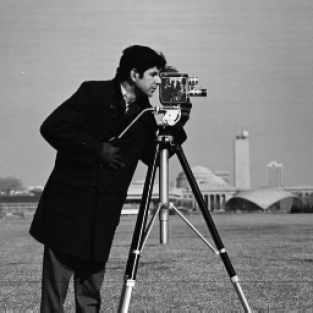
(a) cameraman (256 by 256)

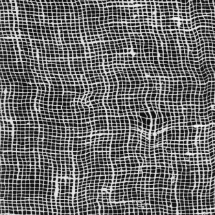
(b) net (640 by 640)

Figure 4: Images used to compare the coding performance of R-K-SVD and the standard K-SVD in Figures 5 and 6.

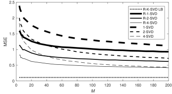
(a) coding error

(b) image patches

(c) K-SVD coding, MSE 0.98

(d) R-K-SVD coding, MSE 0.61

(e) standard atoms

(f) steerable atoms

Figure 5: Coding performance for cameraman based on 17,330 sliding patches. Quantitative comparison of the coding error (a) for K-SVD and R-K-SVD. A qualitative comparison of coding (b-d) and atoms (e,f) is shown for $M=20,K=4$. Red outlines highlight patches where the advantages of R-K-SVD are clearest. Blue outlines show atoms in the standard dictionary that are related by rotation.

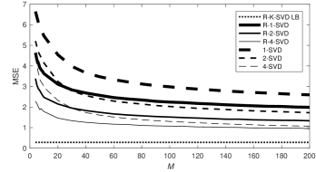
(a) coding error

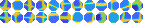
(b) image patches

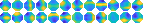
(c) K-SVD coding, MSE 4.13

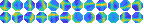
(d) R-K-SVD coding, MSE 2.51

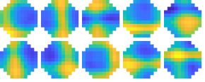
(e) standard atoms

(f) steerable atoms

Figure 6: Coding performance for net based on 396,855 sliding patches. Quantitative comparison of the coding error (a) for K-SVD and R-K-SVD. A qualitative comparison of coding (b-d) and atoms (e,f) is shown for $M=10,K=2$.

Parameter Sensitivity. In a third coding experiment, we study parameter sensitivity with regard to the number of iterations of R-K-SVD and number of angles tested in $[0,2\pi)$ in Fig. 7 and 8, respectively. For both cameraman and net, the optimal performance is reached after 10 iterations and 40 angles tested.

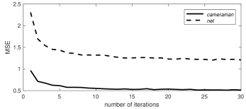
Figure 7: Convergence with respect to the number of iterations (see Figure 2) for $M=20,K=5$.

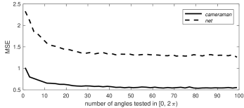
Figure 8: Influence of the number of angles tested in $[0,2\pi)$ for $M=20,K=5$.

III-B Texture Classification

We also explore the advantage of using rotational sparse coding in a texture classification application. Speaking generally, the task is to classify an input image as belonging to one of several texture classes (e.g., sand, pebbles), assuming access to a training set with a number of exemplar images from each class. See Figure 9 for examples of texture classes.

Texture classification is amenable to dictionary learning-based approaches because textures often contain repeated elements (called microtextures or textons) that can be learned. Thus, a dictionary learned on examples of a given class should contain some discriminative information about that class. A set of dictionaries, one learned on each class, should be useful for classification. Our hypothesis is that, in this context, the rotational dictionary should be superior to the standard one because it is able to achieve small coding errors with fewer atoms, meaning that the per-class dictionaries can be very discriminative. Stated another way, we hypothesize that textons repeat not only at different locations, but also with different rotations, and therefore rotational dictionary learning will be able to represent them more easily.

Dataset. We evaluated the texture classification performance on the Outex Database [29]. Outex contains photographs of materials (e.g., fabric, tile) acquired with a standardized protocol. In particular, the Outex_TC_10 validation suite is the most commonly used in the literature and contains 24 texture classes (see Figure 9). Considered texture samples are 128 by 128-pixel images cropped from physically translated and rotated versions of larger samples. The training set contains 480 images including 20 upright samples per class. The test set includes $24$ rotated samples where angles considered are ($5^{\circ}$, $10^{\circ}$, $15^{\circ}$, $30^{\circ}$, $45^{\circ}$, $60^{\circ}$, $75^{\circ}$, and $90^{\circ}$) and where each angle index contains 20 samples per class, resulting in 3840 test images. We expect this to be a good fit for rotational dictionary learning because the construction of the testing set explicitly rewards rotation-invariant methods.

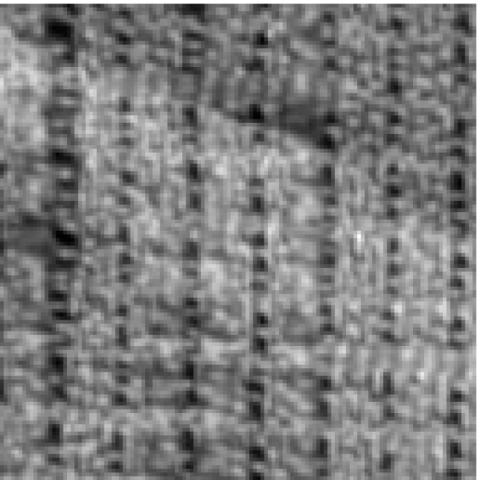
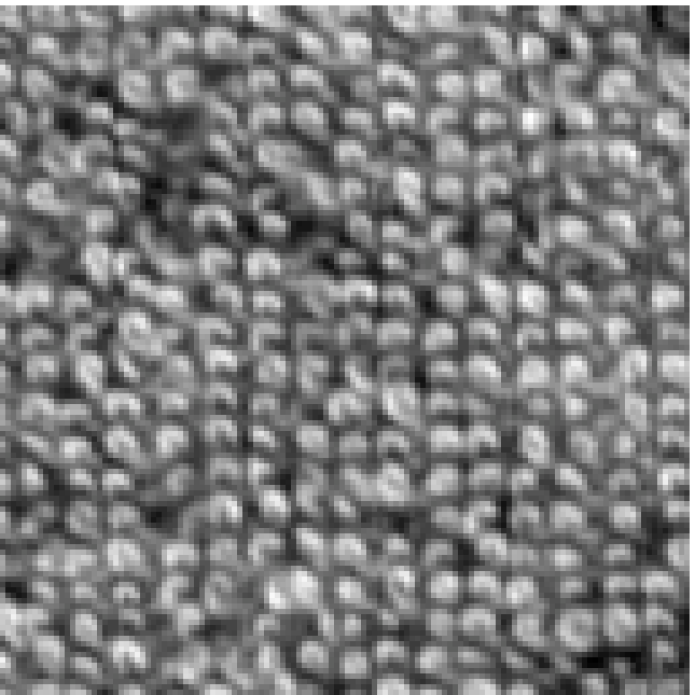
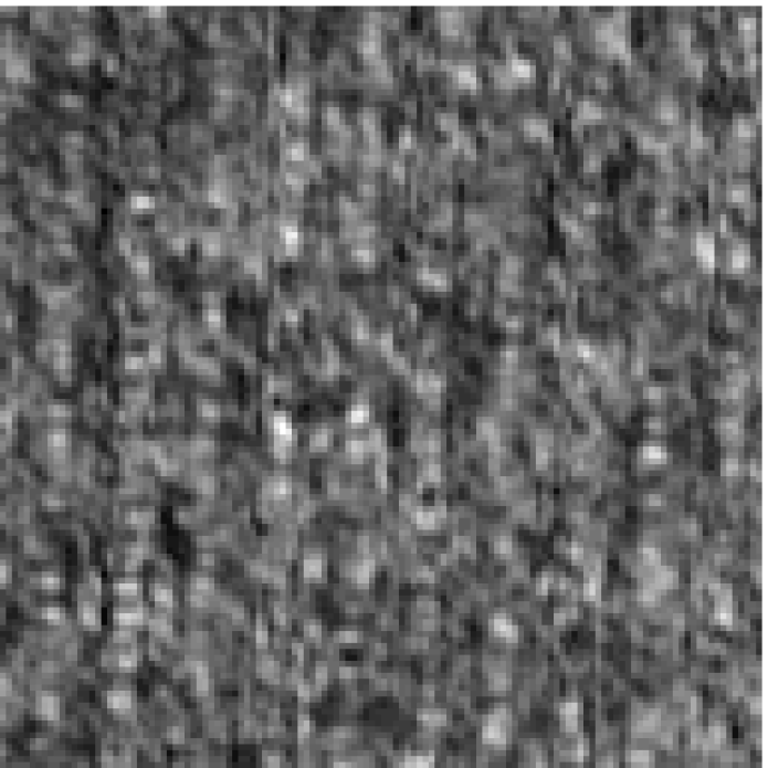
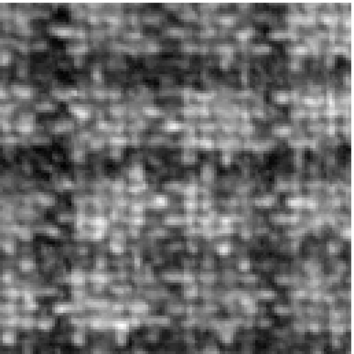
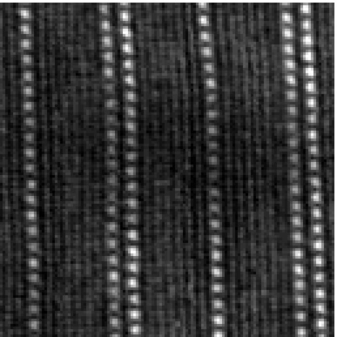
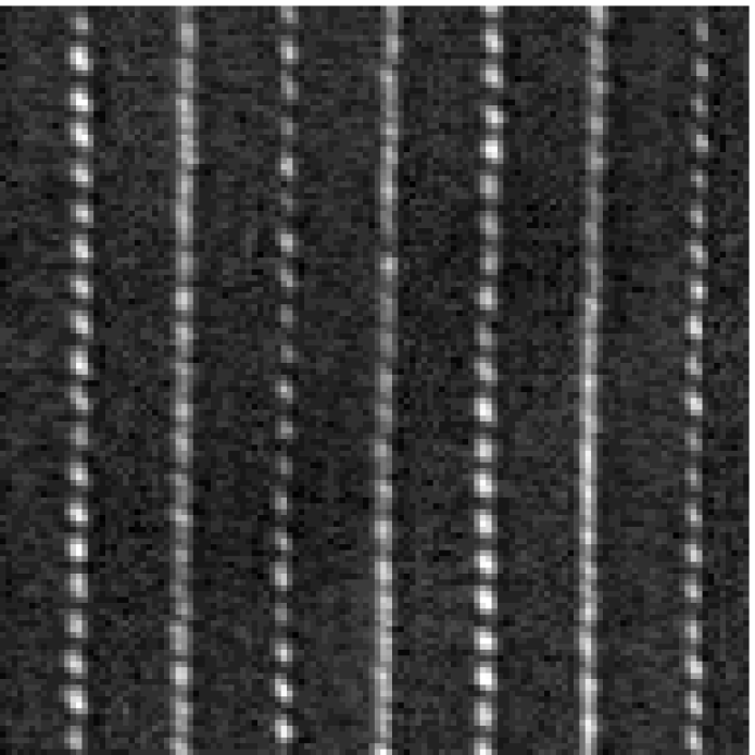
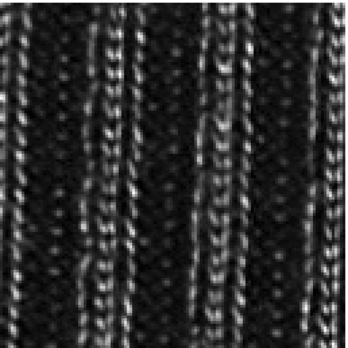
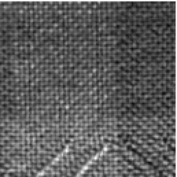
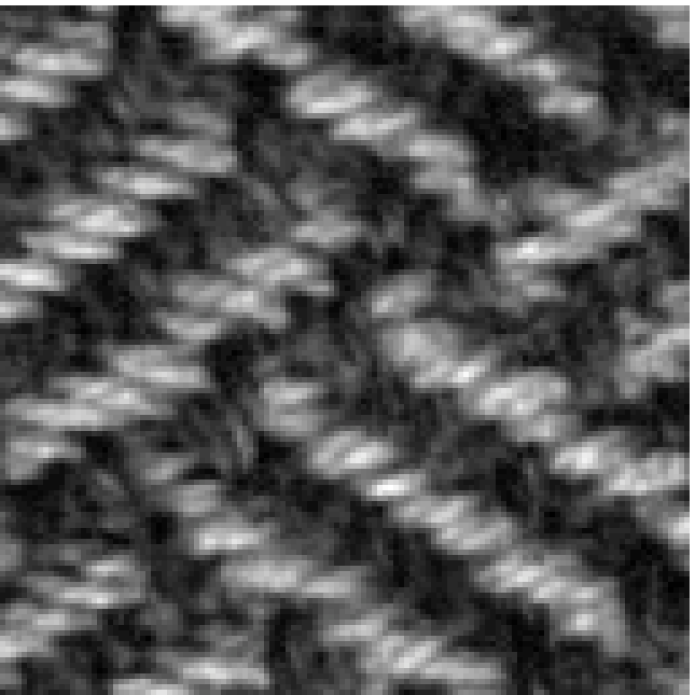
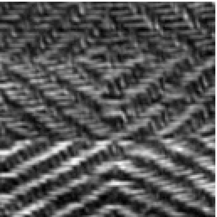
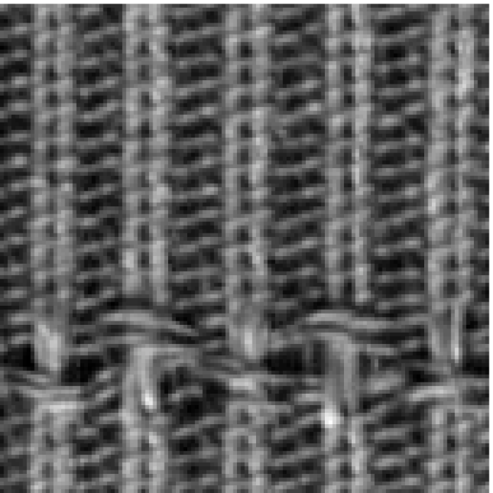
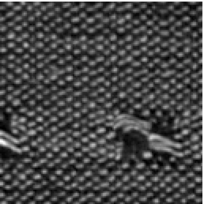
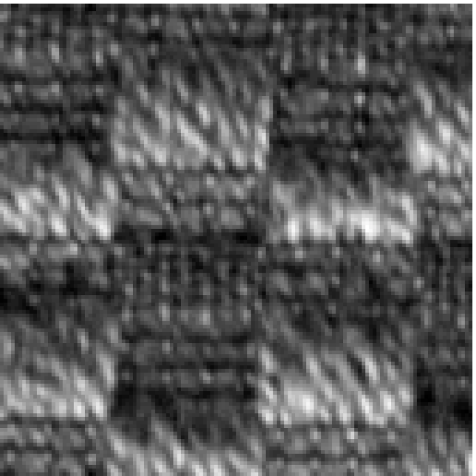
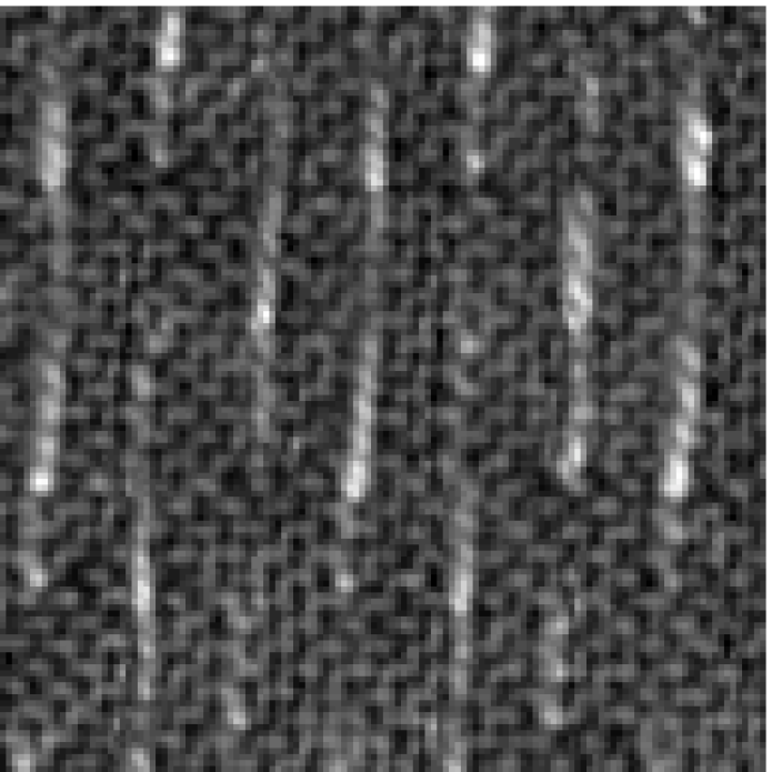
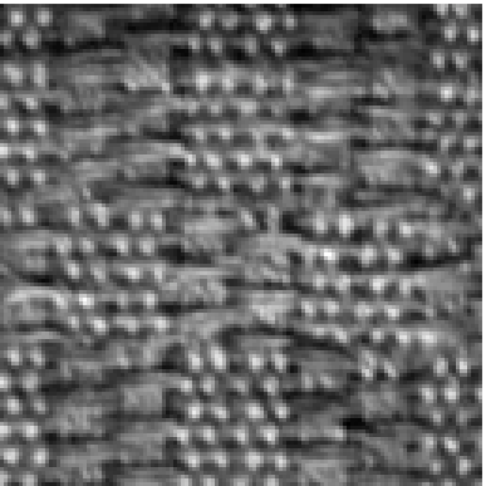
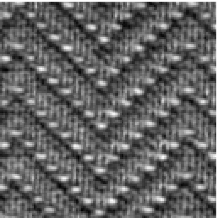
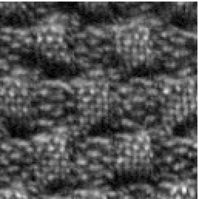
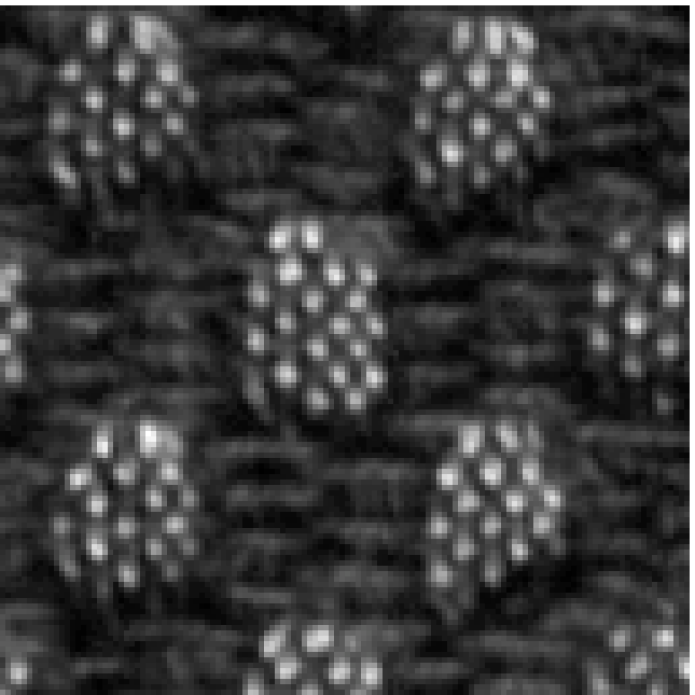
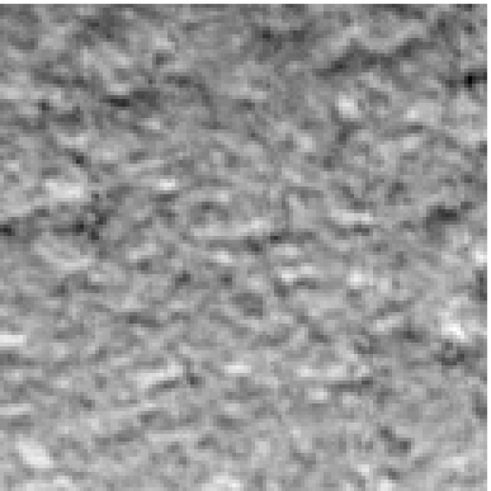
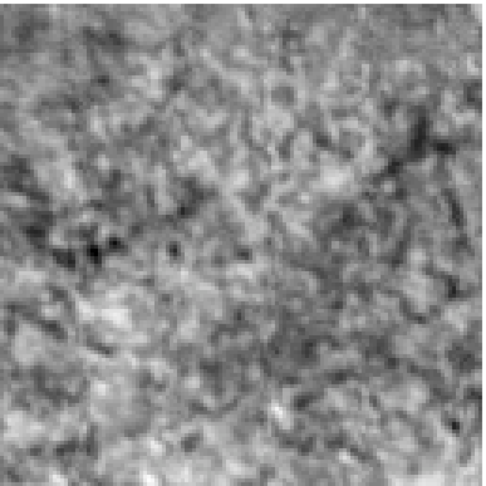
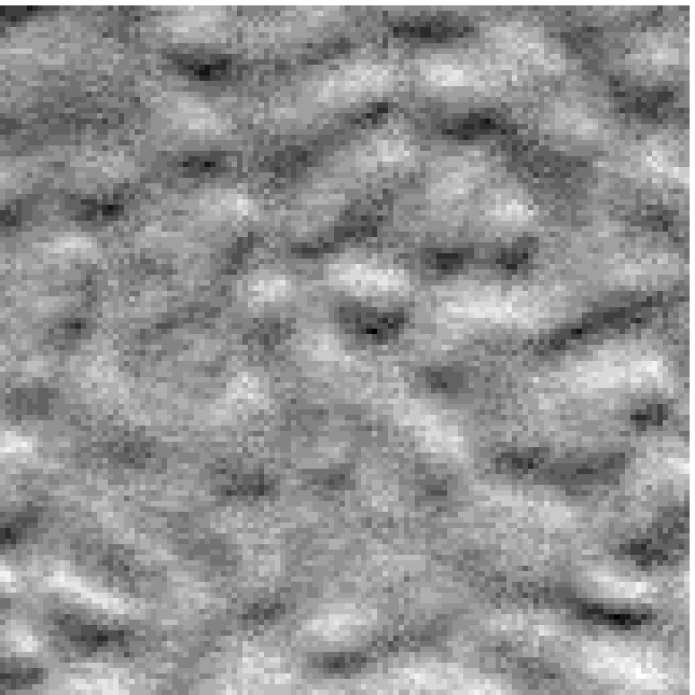
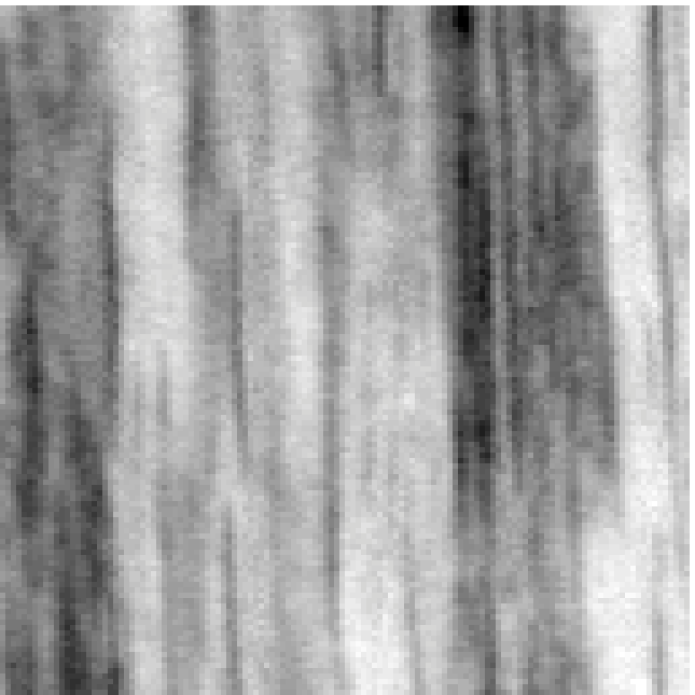
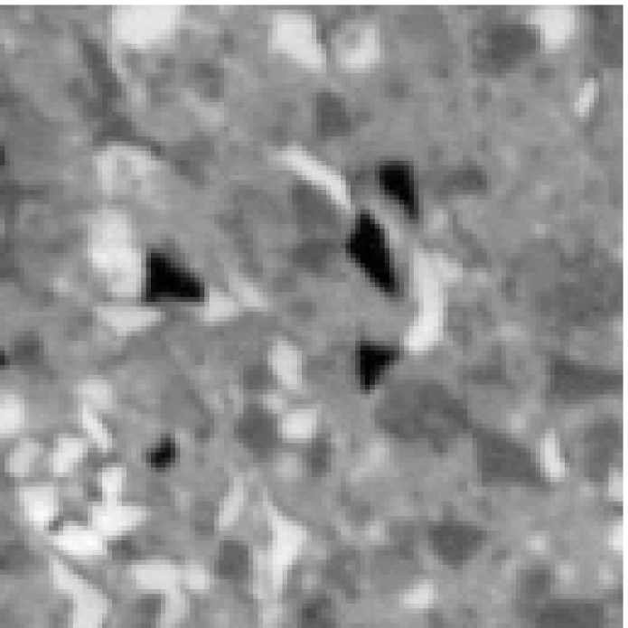
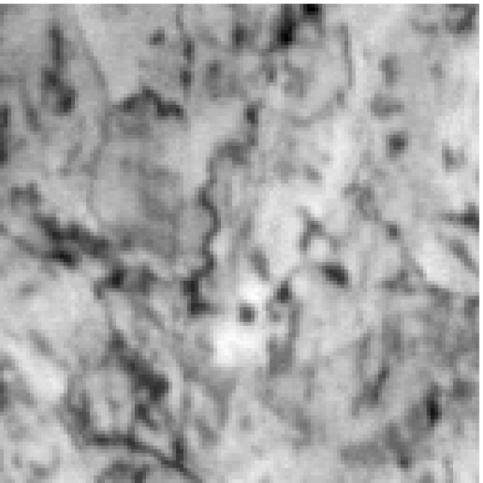
Figure 9: Upright samples of the 24 texture classes included the Outex_TC_10 validation suite. Each image is 128 by 128.

Classifier. Our classification approach is as follows. First, we learn one sparse dictionary per class from the training images. To do this, we split each training image into sliding patches (stride of one pixel). For each class, we randomly select 4,000 of patches from each associated training image resulting in a dataset of 80,000 patches for sparse coding After thus learning one dictionary for each class, we use these dictionaries to code every patch from each training image. For each patch, we assign the class label corresponding to the class dictionary that codes the patch with the minimum sum squared error. We aggregate these patch-level classifications into a histogram for each training image; this histogram is a 24 by 1 feature vector for each training image. To classify a testing image, we form a histogram in the same way and classify the image based on its nearest neighbor in the training set (using the $\chi^{2}$ distance: $d(a,b)=\sum_{i}(a[i]-b[i])^{2}/(a[i]+b[i])$).

We compare three variations of this approach: one using standard sparse coding (K-SVD), one using standard sparse coding with an augmented training set (aug-K-SVD), and one using rotational sparse coding (R-K-SVD). For the augmented approach, during dictionary learning, each training patch takes a random rotation in the set {$5^{\circ}$, $10^{\circ}$, $15^{\circ}$, $30^{\circ}$, $45^{\circ}$, $60^{\circ}$, $75^{\circ}$, $90^{\circ}$}, which mimics the test data. This is a common and effective strategy for adding invariance to classifiers (e.g., artificial neural networks); it essentially teaches the classifier that rotations should be ignored.

For all three approaches, the parameters to set are the size of the dictionary, $M$, the patch size, $N$, and the sparsity level, $K$. These are jointly swept over the values $\{10,25,50,100\}$, $\{11,13,15\}$, and $\{1,2,3\}$, respectively. From these 36 parameter settings, the best combination is selected via cross-validation on the training set: after dictionary learning, a random subset comprising 88% of the training images is held out and classified (the 88% ratio is selected to because it is the ratio of training to test data). This procedure is repeated 100 times and the accuracies of each fold averaged. The parameter setting with the highest average cross-validation accuracy is used during testing. The selected parameters for K-SVD were M=100, N=11, K=3; for augmented K-SVD were M=100, N=15, K=1; and for R-K-SVD were M=100, N=15, K=1.

Comparison methods. While there are numerous published results on Outex (see, e.g., [30] for a table with over a dozen methods from the last two decades), we also ran our own comparisons. Specifically, we compared our approach with current state of the art deep learning frameworks trained end-to-end. We compared seven architectures with and without pretraining and rotational data augmentation (for more details, see Appendix B). The best results, obtained with ResNet50 [31], InceptionV3 [32] and DenseNet169 [33] are reported as comparisons in Table I. As an additional comparison, we used the approach proposed by Cimpoi et al. [34] based on Fisher Vectors and CNNs (FV-CNN). After resampling the images to 231 by 231 using bicubic interpolation, OverFeat [35] was used to extract deep 1024 feature maps from AlexNet (fast model) at the last convolutional layer. FVs were then computed following the setup proposed in [34] with 64 Gaussian mixture components using VLfeat [36]. We retained the first 64 principal components, resulting in a length-64 feature vector for each image. (This length was chosen to maximize testing accuracy; the values we tried were 24, 32, 64, 128, and 256.) We classify testing images by their nearest neighbor in the training set (here using Euclidean distance because the feature vectors are not histograms). We repeat the same procedure for the augmented training set as described in the previous subsection.

Results. We report the results in terms of testing accuracy in Table I. For additional context, we include six recently-reported results—again, see [30] for a more extensive table. The accuracy of our rotational sparse coding-based classifier is 100%, which we believe is the first time a perfect result has been reported for the Outex_TC_10 dataset. The next best result in the literature comes from an artificial neural network-based approach [37], which reports 99.95% (a misclassification of only two testing images), and our implementation of DenseNet169 achieved 99.98 (missing only one testing image). So, while the present results are not a tremendous improvement in accuracy, it is remarkable that our relatively simple approach achieves perfect performance, especially given the number of methods that have been tried. We also show that standard dictionary learning performs significantly better than chance (1/24 = 0.0417), and that augmenting the training set does improve the accuracy. Results for the FV-CNN are significantly better than for the standard dictionary learning, but they do not approach the state of the art, even with data augmentation. This may indicate that, while the FV-CNN captures useful image features, data augmentation alone is not sufficient to provide the rotation invariance needed for Outex. These results indicate that the rotational formulation of dictionary learning is useful in classifying rotation-invariant textures.

TABLE I: Texture classification accuracy on Outex_TC_10

method	accuracy
Hadizadeh 2015 [38]	0.9730
Shrivastava et al. 2015 [39]	0.9919
Zand et al. 2015 [40]	0.9838
Liu et al. 2016 [41]	0.9987
Marcos et al. 2016 [37]	0.9995
Depeursinge et al. 2017 [30]	0.9956
K-SVD	0.4432
aug-K-SVD	0.5635
FV-CNN (64 features) [34]	0.5471
FV-CNN-aug (64 features) [34]	0.6487
ResNet50 [31]	0.9945
InceptionV3 [32]	0.9944
DenseNet169 [33]	0.9983
R-K-SVD	1.0000

• The top seven rows are results reported in other papers. The bottom eight rows are results from experiments in this paper, with our own implementations of the corresponding methods.

To shed more light on the sparse coding methods, we comment here on the results of the parameter sweeps described above—see Table II in Appendix A for the full results. First, the cross-validation accuracy is highest for standard sparse coding, while its testing performance is the lowest. This is consistent with overfitting: because training and validation both occur only on upright images, the standard dictionary fits upright appearance; the other two methods specifically learn in a rotational way, which naturally sacrifices some training performance. Second, the augmented and rotational methods generally benefit from using large patches ($N=15$), while there is no clear trend for the standard method. The underlying tradeoff is that, when larger patches are used, there is effectively less training data (because an image contains fewer independent large patches) and it is higher dimensional (because there are more pixels in each patch). Larger patches also slow down the training and testing stages. Third, all the methods have the highest cross-validation accuracy for the largest dictionary, $M=100$. The dictionary size, $M$, and the sparsity, $K$, control the balance between the representation and discrimination abilities of the dictionary. Larger $M$ and $K$ mean more representation power, which decreases the coding error for patches of the chosen class. But, larger $M$ and $K$ also reduce the coding error for patches outside the chosen class, reducing discrimination. The results suggest that single textures are heterogeneous enough to require a large dictionary to describe them well.

III-C Rotation Speed

In our final experiment, we compare the proposed steering-based patch rotation to standard rotations using interpolation. For a fixed patch size, $N$ by $N$, we form matrices ${\bm{\mathbf{R}}}_{\text{nearest}}$ and ${\bm{\mathbf{R}}}_{\text{bicubic}}$, which are $N^{2}$ by $N^{2}$ matrices that perform a rotation by $100+\sqrt{2}$ degrees using nearest neighbor and bicubic interpolation, respectively. We also create a steerable basis, ${\bm{\mathbf{\Phi}}}$ and steering matrix ${\bm{\mathbf{S}}}$, as described in Section II-D, which achieves the same rotation. Finally, we create a lowpass steerable basis, ${\bm{\mathbf{\Phi}}}_{\text{low}}$, and steering matrix ${\bm{\mathbf{S}}}_{\text{low}}$, where the cutoff frequencies $T_{s}$ have been reduced by half as compared to ${\bm{\mathbf{\Phi}}}$. Thus, for a vectorized patch, ${\bm{\mathbf{x}}}$, rotation can be performed by one of ${\bm{\mathbf{R}}}_{\text{nearest}}{\bm{\mathbf{x}}}$, ${\bm{\mathbf{R}}}_{\text{bicubic}}{\bm{\mathbf{x}}}$, ${\bm{\mathbf{\Phi}}}{\bm{\mathbf{S}}}({\bm{\mathbf{\Phi}}}^{*}{\bm{\mathbf{\Phi}}})^{-1}{\bm{\mathbf{\Phi}}}^{*}{\bm{\mathbf{x}}}$, or ${\bm{\mathbf{\Phi}}}_{\text{low}}{\bm{\mathbf{S}}}_{\text{low}}({\bm{\mathbf{\Phi}}}_{\text{low}}^{*}{\bm{\mathbf{\Phi}}}_{\text{low}})^{-1}{\bm{\mathbf{\Phi}}}_{\text{low}}^{*}{\bm{\mathbf{x}}}$. We compare these four types of rotation on a 51 by 51 patch in Figure 10. The steering-based rotation is qualitatively similar to bicubic interpolation, and it avoids the staircase artifacts present in the nearest neighbor approach. Reducing the cutoff frequencies gives a smoother result.

(a) original

(b) nearest

(c) bicubic

(d) steering

(e) steering${}_{\text{low}}$

Figure 10: Comparison of quality between nearest neighbor, bicubic, and the proposed steering-based rotation. Steering is comparable to bicubic interpolation, while the nearest neighbor interpolation exhibits staircase artifacts.

In order to compare these three rotation methods in the context of the R-K-SVD algorithm, we generate a set of 50,000 random patches and concatenate them into an $N^{2}$ by 50,000 matrix, ${\bm{\mathbf{X}}}$. We then measure the time it takes to left multiply this matrix by ${\bm{\mathbf{R}}}_{\text{nearest}}$ and ${\bm{\mathbf{R}}}_{\text{bicubic}}$. We also compute $\hat{{\bm{\mathbf{X}}}}=({\bm{\mathbf{\Phi}}}^{*}{\bm{\mathbf{\Phi}}})^{-1}{\bm{\mathbf{\Phi}}}^{*}{\bm{\mathbf{X}}}$ and measure the time it takes to left multiply this by ${\bm{\mathbf{S}}}$ (and likewise for ${\bm{\mathbf{\Phi}}}_{\text{low}}$ and ${\bm{\mathbf{S}}}_{\text{low}}$). The rationale for this comparison is that finding $\hat{{\bm{\mathbf{X}}}}$ only occurs once in our algorithm, while the multiplication by ${\bm{\mathbf{R}}}$ or ${\bm{\mathbf{S}}}$ must happen every iteration. All matrix multiplications are done using sparse matrices in Matlab, and timing is performed with the timeit function. The results (Figure 11) show that using steering for rotation is faster than either nearest neighbor or bicubic interpolation, with steering being consistently more than twice as fast as bicubic interpolation.

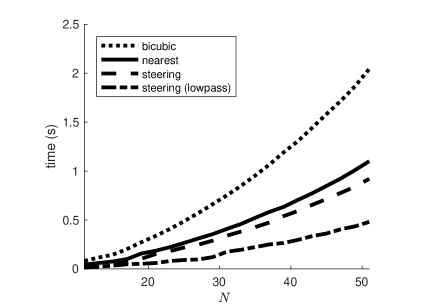
Figure 11: Timing results for rotating 50,000 patches of size $N$ by $N$. Rotation using steerability is significantly faster than bicubic interpolation.

IV Discussions and Conclusion

We presented a novel, fast rotational sparse coding approach based on steerability. Our experiments showed that the rotational formulation provides advantages over the standard sparse coding formulation for coding and texture classification. In particular, its ability to exploit the rotational symmetry of image patches allows the span of the learned dictionary to be reduced without compromising its representational power.

Much of image processing involves either cleverly exploiting or laboring to handle various invariances and equivariances. An excellent example of this theme is convolutional neural networks (CNNs), which, by relying on convolution, both provide useful invariance to translations as well as allow for smaller and faster models than fully-connected networks. For this reason, we believe that the ideas presented here on rotational sparse coding may be useful elsewhere in image processing, especially because the steerable basis can provide a very efficient implementation of rotation in many contexts beyond sparse coding. Indeed, there is already some work on adding steerability to CNNs [42, 43].

The design of discrete steerable bases remains an open topic. It is not clear whether a steerable orthonormal basis can be found, but it is likely that the ad hoc design described in Section II-D can be improved upon. And, even using our specific design, there are several parameters that could be explored further experimentally. We also note that reducing the maximum frequencies provides an easy way to trade rotation quality for speed.

The coding experiments give a sense of how much more expressive rotational sparse coding is than the standard formulation. In particular, we observed for both cameraman and net images that R-K-SVD provides a lower MSE than standard K-SVD, even when the former uses $K=1$ and the latter $K=2$. The visualization of the corresponding atoms and reconstructed patches in Figures 5 and 6 (b-f) shows that R-K-SVD better preserves edge sharpness as no averaging over rotations is happening (see also Fig. 1). We also observed that a standard K-SVD yields atoms that are approximate rotations of each other (e.g., Fig. 5 (e)), meaning that the atom budget is spent on representing rotations of unique patterns.

In our texture classification experiment, we show that a simple classifier based on rotational sparse coding can achieve perfect performance on the Outex_TC_00010 dataset. While modern CNNs can approach this result, they must be pretrained and are not as easy to interpret as the rotational sparse coding model. Our approach is reminiscent of (and partially inspired by) textons [44], with the difference that, here, our textons are not clusters in a feature space, but rather entire dictionaries that encode complicated surfaces. However, our aim is not to promote this specific classifier. Instead, we think the texture classification experiments illustrate a key feature of the rotational formulation of dictionary learning: the tradeoff between representation and discrimination. Because the rotational dictionaries have a better model for the formation of patches, they can lie closer to the true data, allowing accurate representations without a loss of discrimination (i.e., an explosion of the span as discussed with Figure 1). Certainly, tackling challenges like material classification or even texture classification with more intraclass variation, e.g., variations in scale, will require more complicated classification schemes than we discussed here. We see potential in supervised and discriminative sparse coding formulations for learning the atoms, such as those proposed in [45, 46, 47]. In addition, it may be fruitful to combine the rotational formulation, which provides hand-designed invariances, with deep neural networks, which can learn very effective image features, along the lines of the Deep TEN architecture [48] or the rotation invariant CNN in [37].

Appendix A Cross-Validation Results

Table II gives the full results of the parameter sweep described in Section III-B.Classifier and discussed in Section III-B.Results.

Appendix B Deep Learning Comparison Details and Full Results

We compare the results obtained on the Outex_TC_00010 dataset with various state of the art CNN architectures, namely VGG16, VGG19 [49], ResNet50 [31], DenseNet121, DenseNet169, DenseNet201 [33] and InceptionV3 [32]. The networks are either trained from scratch (random weights initialization) or finetuned using weights pre-trained on ImageNet [50]. In both training schemes, the last layer of the networks is replaced by a randomly initialized dense softmax layer with 24 neurons. The Outex images are pre-processed in the same manner as the ImageNet images used for pre-training the networks (generally zero mean and unit variance using ImageNet training set statistics). Note that the input images have to be resized to $224\times 224$ for training and evaluating the VGG16 and VGG19 as these networks require fixed input sizes (no global average pooling). The networks are trained for 100 epochs using an Adam optimizer with categorical cross-entropy and standard hyper-parameters: $\beta_{1}=0.9$, $\beta_{2}=0.999$, batch size $=32$, learning rate $=10^{-4}$, decay rate $=10^{-3}$. The data augmentation employed in these experiments includes random vertical and horizontal flips as well as random rotations in the interval $[0,\pi]$. We used a Keras implementation with TensorFlow backend and trained and evaluated the networks with a Titan Xp graphic card.

Resulting classification performances are reported in Table III. The best result (99.82% accuracy) is achieved with a pre-trained DenseNet121, finetuned and using data augmentation. The top three results are also reported alongside the main results in Table I.

TABLE III: Average accuracy and standard deviation (10 repetitions)

network and training	accuracy
VGG16 scratch	0.4233 $\pm{0.0501}$
VGG16 scratch + data-augm.	0.8968 $\pm{0.0331}$
VGG16 pre-trained	0.5740 $\pm{0.0290}$
VGG16 pre-trained + data-augm.	0.9850 $\pm{0.0067}$
VGG19 scratch	0.3198 $\pm{0.0520}$
VGG19 scratch + data-augm.	0.8431 $\pm{0.0672}$
VGG19 pre-trained	0.5966 $\pm{0.0347}$
VGG19 pre-trained + data-augm.	0.9790 $\pm{0.0074}$
ResNet50 scratch	0.3930 $\pm{0.0413}$
ResNet50 scratch + data-augm.	0.6875 $\pm{0.0635}$
ResNet50 pre-trained	0.8807 $\pm{0.0203}$
ResNet50 pre-trained + data-augm.	0.9945 $\pm{0.0041}$
DenseNet121 scratch	0.6308 $\pm{0.0187}$
DenseNet121 scratch + data-augm.	0.9611 $\pm{0.0158}$
DenseNet121 pre-trained	0.9034 $\pm{0.0102}$
DenseNet121 pre-trained + data-augm.	0.9982 $\pm{0.0016}$
DenseNet169 scratch	0.6520 $\pm{0.0130}$
DenseNet169 scratch + data-augm.	0.9501 $\pm{0.0297}$
DenseNet169 pre-trained	0.9252 $\pm{0.0116}$
DenseNet169 pre-trained + data-augm.	0.9983 $\pm{0.0010}$
DenseNet201 scratch	0.6450 $\pm{0.0202}$
DenseNet201 scratch + data-augm.	0.9621 $\pm{0.0140}$
DenseNet201 pre-trained	0.9401 $\pm{0.0092}$
DenseNet201 pre-trained + data-augm.	0.9980 $\pm{0.0011}$
InceptionV3 scratch	0.6323 $\pm{0.0347}$
InceptionV3 scratch + data-augm.	0.8479 $\pm{0.0324}$
InceptionV3 pre-trained	0.8888 $\pm{0.0248}$
InceptionV3 pre-trained + data-augm.	0.9944 $\pm{0.0018}$

Michael McCann (S’10-M’15) received the B.S.E. in biomedical engineering in 2010 from the University of Michigan and the Ph.D. degree in biomedical engineering from Carnegie Mellon University in 2015. From 2015-2019, he worked with Michael Unser’s group at the École polytechnique fédérale de Lausanne (EPFL). He is currently a Postdoctoral Research Associate with Saiprasad Ravishankar’s group in the Dept. of Computational Mathematics, Science and Engineering at Michigan State University. His research interests center on developing algorithms for biomedical image reconstruction using tools from signal processing, optimization, and machine learning.

Vincent Andrearczyk Vincent Andrearczyk received a double Masters degree in electronics and signal processing from ENSEEIHT, France and Dublin City University, in 2012 and 2013 respectively. He completed his PhD degree on deep learning for texture and dynamic texture analysis at Dublin City University in 2017. He is currently a post-doctoral researcher at the University of Applied Sciences and Arts Western Switzerland with a research focus on deep learning for medical image analysis.

Michael Unser (M’89-SM’94-F’99) is professor and director of EPFL’s Biomedical Imaging Group, Lausanne, Switzerland. His primary area of investigation is biomedical image processing. He is internationally recognized for his research contributions to sampling theory, wavelets, the use of splines for image processing, stochastic processes, and computational bioimaging. He has published over 250 journal papers on those topics. He is the author with P. Tafti of the book An introduction to sparse stochastic processes, Cambridge University Press 2014. From 1985 to 1997, he was with the Biomedical Engineering and Instrumentation Program, National Institutes of Health, Bethesda USA, conducting research on bioimaging. Dr. Unser has held the position of associate Editor-in-Chief (2003-2005) for the IEEE Transactions on Medical Imaging. He is currently member of the editorial boards of SIAM J. Imaging Sciences, IEEE J. Selected Topics in Signal Processing, and Foundations and Trends in Signal Processing. He is the founding chair of the technical committee on Bio Imaging and Signal Processing (BISP) of the IEEE Signal Processing Society. Prof. Unser is a fellow of the IEEE (1999), an EURASIP fellow (2009), and a member of the Swiss Academy of Engineering Sciences. He is the recipient of several international prizes including three IEEE-SPS Best Paper Awards and two Technical Achievement Awards from the IEEE (2008 SPS and EMBS 2010).

Adrien Depeursinge (M’06) Adrien Depeursinge received the B.Sc. and M.Sc. degrees in electrical engineering from the Swiss Federal Institute of Technology (EPFL), Lausanne, Switzerland with a specialization in signal processing. From 2006 to 2010, he performed his Ph.D. thesis on medical image analysis at the University Hospitals of Geneva (HUG). He then spent two years as a Postdoctoral Fellow at the Department of Radiology of the School of Medicine at Stanford University. He has currently a joint position as an Associate Professor at the Institute of Information Systems, University of Applied Sciences Western Switzerland (HES-SO), and as a Senior Research Scientist at EPFL.

References

- [1] I. Tosic and P. Frossard, “Dictionary Learning,” IEEE Signal Processing Magazine, vol. 28, no. 2, pp. 27–38, Mar. 2011.
- [2] K. Engan, S. Aase, and J. Hakon Husoy, “Method of optimal directions for frame design,” in 1999 IEEE International Conference on Acoustics, Speech, and Signal Processing. Proceedings., vol. 5, Phoenix, AZ, Mar. 1999, pp. 2443–2446.
- [3] M. Aharon, M. Elad, and A. Bruckstein, “-SVD: An Algorithm for Designing Overcomplete Dictionaries for Sparse Representation,” IEEE Transactions on Signal Processing, vol. 54, no. 11, pp. 4311–4322, Nov. 2006.
- [4] J. Mairal, F. Bach, J. Ponce, and G. Sapiro, “Online dictionary learning for sparse coding,” in Proceedings of the 26th Annual International Conference on Machine Learning. Montreal, Canada: ACM, Jun. 2009, pp. 689–696.
- [5] K. Skretting and K. Engan, “Recursive least squares dictionary learning algorithm,” IEEE Transactions on Signal Processing, vol. 58, no. 4, pp. 2121–2130, Apr. 2010.
- [6] S. Ravishankar and Y. Bresler, “MR image reconstruction from highly undersampled k-space data by dictionary learning,” IEEE Transactions on Medical Imaging, vol. 30, no. 5, pp. 1028–1041, May 2011.
- [7] Q. Xu, H. Yu, X. Mou, L. Zhang, J. Hsieh, and G. Wang, “Low-dose X-ray CT reconstruction via dictionary learning,” IEEE Transactions on Medical Imaging, vol. 31, no. 9, pp. 1682–1697, Sep. 2012.
- [8] Y. Chen, L. Shi, Q. Feng, J. Yang, H. Shu, L. Luo, J.-L. Coatrieux, and W. Chen, “Artifact suppressed dictionary learning for low-dose CT image processing,” IEEE Transactions on Medical Imaging, vol. 33, no. 12, pp. 2271–2292, Dec. 2014.
- [9] X. Lu, Y. Yuan, and X. Zheng, “Joint dictionary learning for multispectral change detection,” IEEE Transactions on Cybernetics, vol. 47, no. 4, pp. 884–897, Apr. 2017.
- [10] J. Lu, G. Wang, and J. Zhou, “Simultaneous feature and dictionary learning for image set based face recognition,” IEEE Transactions on Image Processing, vol. 26, no. 8, pp. 4042–4054, Aug. 2017.
- [11] T. H. Vu, H. S. Mousavi, V. Monga, G. Rao, and U. K. A. Rao, “Histopathological Image Classification Using Discriminative Feature-Oriented Dictionary Learning,” IEEE Transactions on Medical Imaging, vol. 35, no. 3, pp. 738–751, Mar. 2016.
- [12] Y.-C. Chen, C. S. Sastry, V. M. Patel, P. J. Phillips, and R. Chellappa, “In-plane rotation and scale invariant clustering using dictionaries,” IEEE Transactions on Image Processing, vol. 22, no. 6, pp. 2166–2180, Jun. 2013.
- [13] C. Garcia-Cardona and B. Wohlberg, “Convolutional dictionary learning: A comparative review and new algorithms,” IEEE Transactions on Computational Imaging, vol. 4, no. 3, pp. 366–381, Sep. 2018.
- [14] H. Bristow, A. Eriksson, and S. Lucey, “Fast Convolutional Sparse Coding,” in 2013 IEEE Conference on Computer Vision and Pattern Recognition. IEEE, Jun. 2013, pp. 391–398.
- [15] P. Jost, P. Vandergheynst, S. Lesage, and R. Gribonval, “MoTIF: An Efficient Algorithm for Learning Translation Invariant Dictionaries,” in 2006 IEEE International Conference on Acoustics Speed and Signal Processing Proceedings, vol. 5, Toulouse, France, May 2006, pp. V–857–V–860.
- [16] H. Wersing, J. Eggert, and E. Körner, “Sparse coding with invariance constraints,” in Artificial Neural Networks and Neural Information Processing, Istanbul, Turkey, Jun. 2003, pp. 385–392.
- [17] M. Morup and M. N. Schmidt, “Transformation invariant sparse coding,” in 2011 IEEE International Workshop on Machine Learning for Signal Processing, Santander, Spain, Sep. 2011.
- [18] S. Aeron and E. Kernfeld, “Group-invariant subspace clustering,” in 53rd Annual Allerton Conference on Communication, Control, and Computing, Monticello, IL, Sep. 2015.
- [19] S. Gu, W. Zuo, Q. Xie, D. Meng, X. Feng, and L. Zhang, “Convolutional sparse coding for image super-resolution,” in 2015 IEEE International Conference on Computer Vision (ICCV). IEEE, Dec. 2015.
- [20] B. Wohlberg, “Convolutional sparse representations as an image model for impulse noise restoration,” in 2016 IEEE 12th Image, Video, and Multidimensional Signal Processing Workshop (IVMSP). IEEE, Jul. 2016.
- [21] K. Degraux, U. S. Kamilov, P. T. Boufounos, and D. Liu, “Online convolutional dictionary learning for multimodal imaging,” in 2017 IEEE International Conference on Image Processing (ICIP). Bejing, Chine: IEEE, Sep. 2017.
- [22] E. Simoncelli, W. Freeman, E. Adelson, and D. Heeger, “Shiftable multiscale transforms,” IEEE Transactions on Information Theory, vol. 38, no. 2, pp. 587–607, Mar. 1992.
- [23] M. Unser and N. Chenouard, “A Unifying Parametric Framework for 2d Steerable Wavelet Transforms,” SIAM Journal on Imaging Sciences, vol. 6, no. 1, pp. 102–135, Jan. 2013.
- [24] M. Uenohara and T. Kanade, “Optimal approximation of uniformly rotated images: relationship between karhunen-loeve expansion and discrete cosine transform,” IEEE Transactions on Image Processing, vol. 7, no. 1, pp. 116–119, Jan. 1998.
- [25] O. Chabiron, F. Malgouyres, J.-Y. Tourneret, and N. Dobigeon, “Toward fast transform learning,” International Journal of Computer Vision, vol. 114, no. 2-3, pp. 195–216, Oct. 2014.
- [26] Y. C. Pati, R. Rezaiifar, and P. Krishnaprasad, “Orthogonal matching pursuit: recursive function approximation with applications to wavelet decomposition,” in Proceedings of 27th Asilomar Conference on Signals, Systems and Computers, Pacific Grove, CA, Nov. 1993.
- [27] J. Mairal, F. Bach, and J. Ponce, “Sparse Modeling for Image and Vision Processing,” Foundations and Trends® in Computer Graphics and Vision, vol. 8, no. 2-3, pp. 85–283, Dec. 2014.
- [28] P. Brodatz, Textures: A Photographic Album for Artists and Designers. New York: Dover Publications, Dec. 1966.
- [29] T. Ojala, T. Mäenpää, M. Pietikäinen, J. Viertola, J. Kyllönen, and S. Huovinen, “Outex – new framework for empirical evaluation of texture analysis algorithms,” in 16th International Conference on Pattern Recognition, ser. ICPR, vol. 1. Quebec City, Quebec: IEEE Computer Society, Aug. 2002, pp. 701–706.
- [30] A. Depeursinge, Z. Puspoki, J. P. Ward, and M. Unser, “Steerable wavelet machines (SWM): Learning moving frames for texture classification,” IEEE Transactions on Image Processing, vol. 26, no. 4, pp. 1626–1636, Apr. 2017.
- [31] K. He, X. Zhang, S. Ren, and J. Sun, “Deep residual learning for image recognition,” in Proceedings of the IEEE conference on computer vision and pattern recognition, Las Vegas, NV, Jun. 2016, pp. 770–778.
- [32] C. Szegedy, V. Vanhoucke, S. Ioffe, J. Shlens, and Z. Wojna, “Rethinking the inception architecture for computer vision,” in Proceedings of the IEEE conference on computer vision and pattern recognition, Las Vegas, NV, Jun. 2016, pp. 2818–2826.
- [33] G. Huang, Z. Liu, K. Q. Weinberger, and L. van der Maaten, “Densely connected convolutional networks,” in Proceedings of the IEEE Conference on Computer Vision and Pattern Recognition, Honolulu, HI, Jul. 2017.
- [34] M. Cimpoi, S. Maji, I. Kokkinos, and A. Vedaldi, “Deep Filter Banks for Texture Recognition, Description, and Segmentation,” International Journal of Computer Vision, vol. 118, pp. 65–94, May 2016.
- [35] P. Sermanet, D. Eigen, X. Zhang, M. Mathieu, R. Fergus, and Y. LeCun, “Overfeat: Integrated recognition, localization and detection using convolutional networks,” arXiv:1312.6229 [cs], Dec. 2013.
- [36] A. Vedaldi and B. Fulkerson, “VLFeat: An open and portable library of computer vision algorithms,” http://www.vlfeat.org/, 2008.
- [37] D. Marcos, M. Volpi, and D. Tuia, “Learning rotation invariant convolutional filters for texture classification,” in 2016 23rd International Conference on Pattern Recognition (ICPR), Cancun, Mexico, Dec. 2016.
- [38] H. Hadizadeh, “Noise-resistant and rotation-invariant texture description and representation using local Gabor wavelets binary patterns,” in International Symposium on Artificial Intelligence and Signal Processing (AISP), ser. AISP, Mashhad, Iran, Mar. 2015, pp. 30–34.
- [39] N. Shrivastava and V. Tyagi, “Noise–invariant structure pattern for image texture classification and retrieval,” Multimedia Tools and Applications, pp. 1–20, Jul. 2015.
- [40] M. Zand, S. Doraisamy, A. A. Halin, and M. R. Mustaffa, “Texture classification and discrimination for region–based image retrieval,” Journal of Visual Communication and Image Representation, vol. 26, pp. 305–316, Oct. 2015.
- [41] L. Liu, S. Lao, P. Fieguth, Y. Guo, X. Wang, and M. Pietikäinen, “Median robust extended local binary pattern for texture classification,” IEEE Transactions on Image Processing, vol. 25, no. 3, pp. 1368–1381, Jan. 2016.
- [42] M. Weiler, F. A. Hamprecht, and M. Storath, “Learning steerable filters for rotation equivariant CNNs,” in 2018 IEEE/CVF Conference on Computer Vision and Pattern Recognition, Salt Lake City, UT, Jun. 2018.
- [43] V. Andrearczyk, J. Fageot, V. Oreiller, X. Montet, and A. Depeursinge, “Exploring local rotation invariance in 3D CNNs with steerable filters,” in International Conference on Medical Imaging with Deep Learning, London, England, Jul. 2019.
- [44] J. Malik, S. Belongie, T. Leung, and J. Shi, “Contour and Texture Analysis for Image Segmentation,” International Journal of Computer Vision, vol. 43, no. 1, pp. 7–27, Jun. 2001.
- [45] J. Mairal, F. Bach, J. Ponce, G. Sapiro, and A. Zisserman, “Supervised dictionary learning,” Advances in Neural Information Processing Systems, pp. 1033–1040, 2008.
- [46] Z. Jiang, Z. Lin, and L. S. Davis, “Label consistent k-SVD: Learning a discriminative dictionary for recognition,” IEEE Transactions on Pattern Analysis and Machine Intelligence, vol. 35, no. 11, pp. 2651–2664, Nov. 2013.
- [47] S. Bahrampour, N. M. Nasrabadi, A. Ray, and W. K. Jenkins, “Multimodal task-driven dictionary learning for image classification,” IEEE Transactions on Image Processing, vol. 25, no. 1, pp. 24–38, Jan. 2016.
- [48] H. Zhang, J. Xue, and K. Dana, “Deep TEN: Texture encoding network,” in 2017 IEEE Conference on Computer Vision and Pattern Recognition (CVPR), Honolulu, HI, Jul. 2017.
- [49] K. Simonyan and A. Zisserman, “Very deep convolutional networks for large-scale image recognition,” arXiv preprint arXiv:1409.1556, 2014.
- [50] J. Deng, W. Dong, R. Socher, L.-J. Li, K. Li, and L. Fei-Fei, “ImageNet: A Large-Scale Hierarchical Image Database,” in Proceedings of the IEEE conference on computer vision and pattern recognition, 2009.