The Protein Family Classification in Protein Databases via Entropy Measures

Abstract

In the present work, we review the fundamental methods which have been developed in the last few years for classifying into families and clans the distribution of amino acids in protein databases. This is done through functions of random variables, the Entropy Measures of probabilities of the occurrence of the amino acids. An intensive study of the Pfam databases is presented with restriction to families which could be represented by rectangular arrays of amino acids with m rows (protein domains) and n columns (amino acids). This work is also an invitation to scientific research groups worldwide to undertake the statistical analysis with arrays of different numbers of rows and columns, since we believe in the mathematical characterization of the distribution of amino acids as a fundamental insight on the determination of protein structure and evolution.

1 Introduction and Motivation

DESIDERATA: “To translate the information contained on protein databases in terms of random variables in order to model a dynamics of folding and unfolding of proteins”.

The information on the planetary motion has been annotated on Astronomical almanacs (Ephemerides) along centuries and can be derived and analyzed by Classical Dynamics and Deterministic Chaos as well as confirmed and corrected by General Relativity. The information which is accumulated on Biological almanacs (Protein databases) on the last decades, is still waiting for its first description to be done by a successful theory of folding and unfolding of proteins. We think that this study should be started from the evolution of protein families and its association into Family clans as a necessary step of their development.

The first fundamental idea to be developed here is that proteins do not evolute independently. We introduce several arguments and we have done many calculations to span the bridge over the facts about protein evolution in order to emphasize the existence of a protein family formation process (PFFP), a successful pattern recognition method and a coarse-grained protein dynamics are driven by optimal control theory [1, 2, 3, 4, 5, 6]. Proteins, or their “intelligent” parts, protein domains, evolute together as a family of protein domains. We then realize that the exclusion of the evolution of an “orphan” protein is guaranteed by the probabilistic approach to be introduced in the present contribution. We think that the elucidation of the nature of intermediate stages of the folding/unfolding dynamics, in order to circumvent the Levinthal “paradox” [7, 8] as well as the determination of initial conditions, should be found from a detailed study of this PFFP process. A byproduct of this approach is the possibility of testing the hypothesis of agglutination of protein families into Clans by rigorous statistical methods like ANOVA [9, 4].

We take many examples of Entropy Measures as the generalized functions of random variables on our modelling. These are the probabilities of occurrence of amino acids in rectangular arrays which are the representatives of families of protein domains. In section 2, the sample space which is adequate for this statistical approach is described in detail. We start from the definition of probabilities of occurrence and the restrictions imposed on the number of feasible families by the structure of this sample space. Section 3 introduces the set of Sharma-Mittal Entropy Measures [10, 4] to be adopted as the functions of probabilities of occurrence in the statistical analysis to be developed. The Mutual Information measures associated with the Sharma-Mittal set, as well as the normalized Jaccard distance measures, are also introduced in this section. In section 4, we present a naive sketch of assessing Protein database, to set the stage for a more efficient approach of the following sections. In section 5, we point out the inconvenience of the Maple computing system for the statistical calculations to be done, by displaying tables with all CPU and real times necessary to perform all necessary calculations. We have also provided in this section, some adaptation of our methods in order to be used with the Perl computing system and we compare the new times of calculation with those by using Maple at the beginning of the section. We also include some comments on the use of Perl, especially on its oddness to calculate with the input data given in arrays and the way of circumventing this. However, we also stress that despite the fact that joint probabilities and their powers could be usually calculated, the output will come randomly distributed and the CPU and real times will increase too much to favour the calculation of the entropy measures. This is due to the intrinsic “Hash” structure [11] of the Perl computing system. We then introduce a modified array structure in order to calculate with Perl.

2 The Sample Space for a Statistical Treatment

We consider a rectangular array of m rows (protein domains) and n columns (amino acids). These arrays are organized from the protein database whose domains are classified into families and clans by the professional expertise of senior biologists [12, 13].

The random variable is the probability of occurrences of amino acids, $p_{j}(a)$, $j=1,2,\ldots,n$, $a=A,C,D,\ldots,W,Y$ (one-letter code for amino acids), to be given by

$$p_{j}(a)\equiv\frac{n_{j}(a)}{m}$$ (1)

where $n_{j}(a)$ is the number of occurrences of the amino acid a in the $j$-th column. Eq.(1) could be also interpreted as the components of n vectors of 20 components each

$$\begin{pmatrix}p_{1}(A)\\ \vdots\\ p_{1}(Y)\end{pmatrix}\begin{pmatrix}p_{2}(A)\\ \vdots\\ p_{2}(Y)\end{pmatrix}\ldots\begin{pmatrix}p_{n}(A)\\ \vdots\\ p_{n}(Y)\end{pmatrix}$$ (2)

and we have

$$\sum_{a}n_{j}(a)=m\,,\,\,\forall j\,\Rightarrow\,\sum_{a}p_{j}(a)=1\,,\,\,\forall j$$ (3)

Analogously, we could also introduce the joint probability of occurrence of a pair of amino acids a, b in columns j, k, respectively $P_{jk}(a,b)$ as the random variables. These are given by

$$P_{jk}(a,b)=\frac{n_{jk}(a,b)}{m}$$ (4)

where $n_{jk}(a,b)$ is the number of occurrences of the pair of amino acids a, b in columns j, k, respectively.

A convenient interpretation of these joint probabilities could be the elements of $\frac{n(n-1)}{2}$, square matrices of $20\times 20$ elements, to be written as

$$P_{jk}=\begin{pmatrix}P_{jk}(A,A)&\ldots&P_{jk}(A,Y)\\ \vdots&\ddots&\vdots\\ P_{jk}(Y,A)&\ldots&P_{jk}(Y,Y)\end{pmatrix}$$ (5)

where $j=1,2,\ldots,(n-1)$; $k=j+1,\ldots,n$.

We can also write,

$$P_{jk}(a,b)=P_{jk}(a|b)p_{k}(b)\,,$$ (6)

This equation can be also taken as another definition of joint probability. $\!P\!_{jk}(\!a|b)$ is the Conditional probability of occurrence of the amino acid a in column j if the amino acid b is already found in column k. We then have,

$$\sum_{a}P_{jk}(a|b)=1$$ (7)

From eqs.(6), (7), we have:

$$\sum_{a}P_{jk}(a,b)=p_{k}(b)$$ (8)

and from eq.(8),

$$\sum_{a}\sum_{b}P_{jk}(a,b)=1$$ (9)

which is an identity since $P_{jk}(a,b)$ is also a probability.

Eqs.(8) and (9) can be also derived from

$$\sum_{a}n_{jk}(a,b)=n_{k}(b)\,;\quad\sum_{a}\sum_{b}n_{jk}(a,b)=m$$ (10)

and the definitions, eqs.(1), (4).

We now have from Bayes’ law:

$$P_{jk}(a|b)p_{k}(b)=P_{kj}(b|a)p_{j}(a)$$ (11)

and from eq.(11), the property of symmetry,

$$P_{jk}(a,b)=P_{kj}(b,a)$$ (12)

The matrices $P_{jk}$ can be organized in a triangular array:

$$P=\begin{matrix}{}&P_{12}&P_{13}&P_{14}&\ldots&P_{1\,n-2}&P_{1\,n-1}&P_{1\,n}\\ {}&{}&P_{23}&P_{24}&\ldots&P_{2\,n-2}&P_{2\,n-1}&P_{2\,n}\\ {}&{}&{}&P_{34}&\ldots&P_{3\,n-2}&P_{3\,n-1}&P_{3\,n}\\ {}&{}&{}&{}&\ddots&\vdots&\vdots&\vdots\\ {}&{}&{}&{}&{}&P_{n-3\,n-2}&P_{n-3\,n-1}&P_{n-3\,n}\\ {}&{}&{}&{}&{}&{}&P_{n-2\,n-1}&P_{n-2\,n}\\ {}&{}&{}&{}&{}&{}&{}&P_{n-1\,n}\end{matrix}$$ (13)

The number of matrices until the $P_{jk}$-th one is given by

$$C_{jk}=j(n-1)-\frac{j(j-1)}{2}-(n-k)$$ (14)

These numbers can be also arranged as a triangular array:

Eq.(13) should be used for the construction of a computational code to perform all necessary calculations. We postpone to other publication the presentation of some interesting results on the analysis of eq.(15).

The calculation of the matrix elements $P_{jk}(a,b)$ from a rectangular array $m\times n$ of amino acids is done by the “concatenation” process which is easily implemented on computational codes. We choose a pair of columns $j=\bar{\jmath}$, $k=\bar{k}$ from the strings, $a=A$, $C$, $\ldots$, $W$, $Y$, $b=A$, $C$, $\ldots$, $W$, $Y$ and we look for the occurrence of the combinations $ab=AA$, $AC$, $\ldots$, $AW$, $AY$, $CA$, $CC$, $\ldots$, $CW$, $CY$, $\ldots$, $WA$, $WC$, $\ldots$, $WW$, $WY$, $\ldots$, $YA$, $YC$, $\ldots$, $YW$, $YY$. We then calculate their numbers of occurrences $n_{\bar{\jmath}\bar{k}}(A,A)$, $n_{\bar{\jmath}\bar{k}}(A,C)$, $\ldots$, $n_{\bar{\jmath}\bar{k}}(Y,W)$, $n_{\bar{\jmath}\bar{k}}(Y,Y)$ and the corresponding probabilities $P_{\bar{\jmath}\bar{k}}(A,A)$, $P_{\bar{\jmath}\bar{k}}(A,C)$, $\ldots$,
$P_{\bar{\jmath}\bar{k}}(Y,W)$, $P_{\bar{\jmath}\bar{k}}(Y,Y)$ from eq.(4). We do the same for the other $\frac{n^{2}-n-2}{2}$ pairs of columns.

As an example, let us suppose that we have the $3\times 4$ array:

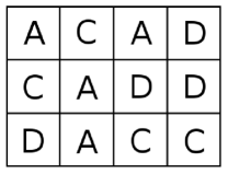
Figure 1: An example of a $3\times 4$ array with amino acids A, C, D.

Let us choose the pair of columns 1,2. We look for the occurrence of the combinations $AA$, $AC$, $AD$, $CA$, $CC$, $CD$, $DA$, $DC$, $DD$ on the pair of columns 1,2 of the array above and we found $n_{12}(A,C)=1$, $n_{12}(C,A)=1$, $n_{12}(D,A)=1$. The others $n_{12}(a,b)=0$. From eq.(4) we can write for the matrices $P_{jk}$ of eq.(5):

$$P_{12}=\begin{pmatrix}0&1/3&0\\ 1/3&0&0\\ 1/3&0&0\end{pmatrix}\!;P_{13}=\begin{pmatrix}1/3&0&0\\ 0&0&1/3\\ 0&1/3&0\end{pmatrix}\!;P_{14}=\begin{pmatrix}0&0&1/3\\ 0&0&1/3\\ 0&1/3&0\end{pmatrix}$$

$$P_{23}=\begin{pmatrix}0&1/3&1/3\\ 1/3&0&0\\ 0&0&0\end{pmatrix}\!;P_{24}=\begin{pmatrix}0&1/3&1/3\\ 0&0&1/3\\ 0&0&0\end{pmatrix}\!;P_{34}=\begin{pmatrix}0&0&1/3\\ 0&1/3&0\\ 0&0&1/3\end{pmatrix}$$ (16)

The Maple computing system “recognizes” the matricial structure through its Linear Algebra package. The Perl computing system “operates” only with “strings”. The results above are easily obtained in Maple, but in Perl we have to find alternative ways of calculating the joint probabilities. The first method is to calculate the probabilities per row of the $3\times 4$ array. We have for the first row:

$$\Pi_{12}^{(1)}=\begin{pmatrix}0&1/3&0\\ 0&0&0\\ 0&0&0\end{pmatrix}\!;\,\,\Pi_{13}^{(1)}=\begin{pmatrix}1/3&0&0\\ 0&0&0\\ 0&0&0\end{pmatrix}\!;\,\,\Pi_{14}^{(1)}=\begin{pmatrix}0&0&1/3\\ 0&0&0\\ 0&0&0\end{pmatrix}$$

$$\Pi_{23}^{(1)}=\begin{pmatrix}0&0&0\\ 1/3&0&0\\ 0&0&0\end{pmatrix}\!;\,\,\Pi_{24}^{(1)}=\begin{pmatrix}0&0&0\\ 0&0&1/3\\ 0&0&0\end{pmatrix}\!;\,\,\Pi_{34}^{(1)}=\begin{pmatrix}0&0&1/3\\ 0&0&0\\ 0&0&0\end{pmatrix}$$ (17)

For the second row:

$$\Pi_{12}^{(2)}=\begin{pmatrix}0&0&0\\ 1/3&0&0\\ 0&0&0\end{pmatrix}\!;\,\,\Pi_{13}^{(2)}=\begin{pmatrix}0&0&0\\ 0&0&1/3\\ 0&0&0\end{pmatrix}\!;\,\,\Pi_{14}^{(2)}=\begin{pmatrix}0&0&0\\ 0&0&1/3\\ 0&0&0\end{pmatrix}$$

$$\Pi_{23}^{(2)}=\begin{pmatrix}0&0&1/3\\ 0&0&0\\ 0&0&0\end{pmatrix}\!;\,\,\Pi_{24}^{(2)}=\begin{pmatrix}0&0&1/3\\ 0&0&0\\ 0&0&0\end{pmatrix}\!;\,\,\Pi_{34}^{(2)}=\begin{pmatrix}0&0&0\\ 0&0&0\\ 0&0&1/3\end{pmatrix}$$ (18)

For the third row:

$$\Pi_{12}^{(3)}=\begin{pmatrix}0&0&0\\ 0&0&0\\ 1/3&0&0\end{pmatrix}\!;\,\,\Pi_{13}^{(3)}=\begin{pmatrix}0&0&0\\ 0&0&0\\ 0&1/3&0\end{pmatrix}\!;\,\,\Pi_{14}^{(3)}=\begin{pmatrix}0&0&0\\ 0&0&0\\ 0&1/3&0\end{pmatrix}$$

$$\Pi_{23}^{(3)}=\begin{pmatrix}0&1/3&0\\ 0&0&0\\ 0&0&0\end{pmatrix}\!;\,\,\Pi_{24}^{(3)}=\begin{pmatrix}0&1/3&0\\ 0&0&0\\ 0&0&0\end{pmatrix}\!;\,\,\Pi_{34}^{(3)}=\begin{pmatrix}0&0&0\\ 0&1/3&0\\ 0&0&0\end{pmatrix}$$ (19)

We stress that Perl does not recognize these matrix structures. This is just our arrangement in order to make comparison with Maple calculations. However, Perl “knows” how to sum the calculations done per rows to obtain:

$$\Pi_{12}^{(1)}+\Pi_{12}^{(2)}+\Pi_{12}^{(3)}=\begin{pmatrix}0&1/3&0\\ 1/3&0&0\\ 1/3&0&0\end{pmatrix}\equiv P_{12}$$ (20)

$$\Pi_{13}^{(1)}+\Pi_{13}^{(2)}+\Pi_{13}^{(3)}=\begin{pmatrix}1/3&0&0\\ 0&0&1/3\\ 0&1/3&0\end{pmatrix}\equiv P_{13}$$ (21)

$$\Pi_{14}^{(1)}+\Pi_{14}^{(2)}+\Pi_{14}^{(3)}=\begin{pmatrix}0&0&1/3\\ 0&0&1/3\\ 0&1/3&0\end{pmatrix}\equiv P_{14}$$ (22)

$$\Pi_{23}^{(1)}+\Pi_{23}^{(2)}+\Pi_{23}^{(3)}=\begin{pmatrix}0&1/3&1/3\\ 1/3&0&0\\ 0&0&0\end{pmatrix}\equiv P_{23}$$ (23)

$$\Pi_{24}^{(1)}+\Pi_{24}^{(2)}+\Pi_{24}^{(3)}=\begin{pmatrix}0&1/3&1/3\\ 0&0&1/3\\ 0&0&0\end{pmatrix}\equiv P_{24}$$ (24)

$$\Pi_{34}^{(1)}+\Pi_{34}^{(2)}+\Pi_{34}^{(3)}=\begin{pmatrix}0&0&1/3\\ 0&1/3&0\\ 0&0&1/3\end{pmatrix}\equiv P_{34}$$ (25)

We are then able to translate the Perl output in “matrix language”. However, this output does not come as an ordered set of joint probabilities, as we have done by arranging the output in the form of the matrices $\Pi_{jk}^{(l)}$, $j=1,2,3$, $k=2,3,4$, $l=1,2,3$. In order to calculate functions of the probabilities as the entropy measures, it will take too much time for the Perl computing system to collect the necessary probability values. This is due to the “Hash” structure of the Perl as compared to the usual “array” structure of the Maple. A new form of arranging the strings to favour an a priori ordination will circumvent this inconvenience of the “hash” structure. Let us then write the following extended string associated to the $m\times n$ rectangular array:

$$\Big{(}\underbrace{(\overset{1}{A}\overset{2}{C}\overset{3}{D})}_{1}\underbrace{(\overset{1}{C}\overset{2}{A}\overset{3}{A})}_{2}\underbrace{(\overset{1}{A}\overset{2}{D}\overset{3}{C})}_{3}\underbrace{(\overset{1}{D}\overset{2}{D}\overset{3}{C})}_{4}\Big{)}$$

We then get

$$P_{12}(A,C)=1/3,\quad P_{12}(C,A)=1/3,\quad P_{12}(D,A)=1/3$$

$$P_{13}(A,A)=1/3,\quad P_{13}(C,D)=1/3,\quad P_{13}(D,C)=1/3$$

$$P_{14}(A,D)=1/3,\quad P_{14}(C,D)=1/3,\quad P_{14}(D,C)=1/3$$

$$P_{23}(C,A)=1/3,\quad P_{23}(A,D)=1/3,\quad P_{23}(A,C)=1/3$$

$$P_{24}(C,D)=1/3,\quad P_{24}(A,D)=1/3,\quad P_{24}(A,C)=1/3$$

$$P_{34}(A,D)=1/3,\quad P_{34}(D,D)=1/3,\quad P_{34}(C,C)=1/3$$ (26)

All the other joint probabilities $P_{jk}(a,b)$ are equal to zero.

This is a feasible treatment for the “hash” structure. In the example solved above the probabilities will come already ordered in triads. This will save time in the calculations with the Perl system.

It should be stressed that the Perl computing system does not recognize any formal relations of Linear Algebra. However, it does quite well if these relations are converted into products and sums. In order to give an example of working with the Perl system, we take a calculation with the usual Shannon Entropy measure. The calculation of the Entropy for the columns $j$,$k$ is done by

$$S_{jk}=-\sum_{a}\sum_{b}P_{jk}(a,b)\log P_{jk}(a,b)=-\mathrm{Tr}\Big{(}P_{jk}(\log P_{jk})^{\mathrm{T}}\Big{)}$$ (27)

where $P_{jk}$ is the matrix given in eq.(5) and $\mathrm{Tr,T}$ stands for the operations of taking the trace and transposing a matrix, respectively. The matrix $(\log P_{jk})^{\mathrm{T}}$ is given by

$$(\log P_{jk})^{\mathrm{T}}=\begin{pmatrix}\log P_{jk}(A,A)&\ldots&\log P_{jk}(Y,A)\\ \vdots&{}&\vdots\\ \log P_{jk}(A,Y)&\ldots&\log P_{jk}(Y,Y)\end{pmatrix}$$

we also include for a useful reference, the matrix

$$p_{j}(p_{k})^{\mathrm{T}}=\begin{pmatrix}p_{j}(A)p_{k}(A)&\ldots&p_{j}(A)p_{k}(Y)\\ \vdots&{}&\vdots\\ p_{j}(Y)p_{k}(A)&\ldots&p_{j}(Y)p_{k}(Y)\end{pmatrix}$$

Since from eqs.(20)–(25), we have

$$P_{jk}=\sum_{l=1}^{m}\Pi_{jk}^{(l)}$$ (28)

we can write:

$$S_{jk}=-\mathrm{Tr}\left(\left(\sum_{l=1}^{m}\Pi_{jk}^{(l)}\right)(\log P_{jk})^{\mathrm{T}}\right)=-\sum_{l=1}^{m}\mathrm{Tr}\Big{(}\Pi_{jk}^{(l)}(\log P_{jk})^{\mathrm{T}}\Big{)}$$ (29)

There is no problem for calculating in Perl, if we prepare eq.(28) by expressing previously all the products and sums to be done. The real problem with Perl calculations is the arrangement of the output of values $P_{jk}(a,b)$, due to the “hash” structure as have been stressed above.

3 Entropy Measures. The Sharma-Mittal set and the associated Jaccard Entropy measure

We start this section with the definition of the two-parameter Sharma-Mittal entropies [10, 1, 2]

$$(SM)_{jk}(r,s) =-\frac{1}{1-r}\left(1-\left(\sum_{a}\sum_{b}\big{(}P_{jk}(a,b)\big{)}^{s}\right)^{\frac{1-r}{1-s}}\right)$$ (30)

$$(SM)_{j}(r,s) =-\frac{1}{1-r}\left(1-\left(\sum_{a}\big{(}p_{j}(a)\big{)}^{s}\right)^{\frac{1-r}{1-s}}\right)$$ (31)

where $p_{j}(a)$ and $P_{jk}(a,b)$ are the simple and joint probabilities of occurrence of amino acids as defined on eqs.(1) and (4), respectively. r, s are non-dimensional parameters.

We can associate to the entropy measures above their corresponding one parameter forms to be given by the limits:

$$H_{jk}(s) =\lim_{r\to s}(SM)_{jk}(r,s)=-\frac{1}{1-s}\left(1-\sum_{a}\sum_{b}\big{(}P_{jk}(a,b)\big{)}^{s}\right)$$ (32)

$$H_{j}(s) =\lim_{r\to s}(SM)_{j}(r,s)=-\frac{1}{1-s}\left(1-\sum_{a}\big{(}p_{j}(a)\big{)}^{s}\right)$$ (33)

These are the Havrda-Charvat Entropy Measures and they will be specially emphasized in the present work. Other alternative proposals for the single parameter entropies are given by

The Renyi’s Entropy measures:

$$R_{jk}(s) =\lim_{r\to 1}(SM)_{jk}(r,s)=\frac{1}{1-s}\log\left(\sum_{a}\sum_{b}\big{(}P_{jk}(a,b)\big{)}^{s}\right)$$ (34)

$$R_{j}(s) =\lim_{r\to 1}(SM)_{j}(r,s)=\frac{1}{1-s}\log\left(\sum_{a}\big{(}p_{j}(a)\big{)}^{s}\right)$$ (35)

The Landsberg-Vedral Entropy measures:

$$L_{jk}(s)=\!\lim_{\quad r\to 2-s}(SM)_{jk}(r,s) =\frac{1}{1-s}\left(1-\Big{(}\sum_{a}\sum_{b}\big{(}P_{jk}(a,b)\big{)}^{s}\Big{)}^{-1}\right)$$ (36)

$$=\frac{H_{jk}(s)}{\sum\limits_{a}\sum\limits_{b}\big{(}P_{jk}(a,b)\big{)}^{s}}$$

$$L_{j}(s)=\!\lim_{\quad r\to 2-s}(SM)_{j}(r,s) =\frac{1}{1-s}\left(1-\Big{(}\sum_{a}\big{(}p_{j}(a)\big{)}^{s}\Big{)}^{-1}\right)$$ (37)

$$=\frac{H_{j}(s)}{\sum\limits_{a}\big{(}p_{j}(a)\big{)}^{s}}$$

All these Entropy measures have the free-parameter Shannon entropy in the limit $s\to 1$.

$$\lim_{s\to 1}H_{jk}(s) =\lim_{s\to 1}R_{jk}(s)=\lim_{s\to 1}L_{jk}(s)=S_{jk}$$ (38)

$$\lim_{s\to 1}H_{j}(s) =\lim_{s\to 1}R_{j}(s)=\lim_{s\to 1}L_{j}(s)=S_{j}$$ (39)

where

$$S_{jk} =-\sum_{a}\sum_{b}P_{jk}(a,b)\log P_{jk}(a,b)$$ (27)

$$S_{j} =-\sum_{a}p_{j}(a)\log p_{j}(a)$$ (40)

are the Shannon entropy measures [6].

We now introduce a convenient version of a Mutual Information measure:

$$M_{jk}(r,s)=\frac{1}{1-r}\left(1-\left(\frac{\sum\limits_{a}\sum\limits_{b}\big{(}P_{jk}(a,b)\big{)}^{s}}{\sum\limits_{a}\sum\limits_{b}\big{(}p_{j}(a)p_{k}(b)\big{)}^{s}}\right)^{\frac{1-r}{1-s}}\right)$$ (41)

We can see that $M_{jk}(r,0)=0$ and if $\exists\,\bar{\jmath},\bar{k}$ such that $P_{\bar{\jmath}\bar{k}}(a,b)=p_{\bar{\jmath}}(a)p_{\bar{k}}(b)$ $\Rightarrow$ $M_{\bar{\jmath}\bar{k}}(r,s)=0$. We also have,

$$M_{jk}(1,s)=\lim_{r\to 1}M_{jk}(r,s)=-\frac{1}{1-s}\log\left(\frac{\sum\limits_{a}\sum\limits_{b}\big{(}P_{jk}(a,b)\big{)}^{s}}{\sum\limits_{a}\sum\limits_{b}\big{(}p_{j}(a)p_{k}(b)\big{)}^{s}}\right)$$ (42)

and in the limit $s\to 1$

$$M_{jk}=\lim_{s\to 1}M_{jk}(1,s)= \sum_{a}\sum_{b}P_{jk}(a,b)\log P_{jk}(a,b)$$

$$-\sum_{a}\sum_{b}p_{j}(a)p_{k}(b)\log\big{(}p_{j}(a)p_{k}(b)\big{)}$$ (43)

and from the identities:

$$\sum_{a}p_{j}(a)=1\,,\,\forall j\,;\quad\sum_{b}p_{k}(b)=1\,,\,\forall k$$

$$\sum_{a}P_{jk}(a,b)=p_{k}(b)\,,\,\forall j\,;\quad\sum_{b}P_{jk}(a,b)=p_{j}(a)\,,\,\forall k$$

obtained from eqs.(3), (4), (6), (7), we can also write instead eq.(43):

$$M_{jk}=\sum_{a}\sum_{b}P_{jk}(a,b)\log P_{jk}(a,b)-\sum_{a}\sum_{b}P_{jk}(a,b)\log\big{(}p_{j}(a)p_{k}(b)\big{)}$$ (44)

It should be stressed that we are not assuming that $P_{jk}(a,b)\equiv p_{j}(a)p_{k}(b)$ above. This equality is assumed to be valid only for $j=\bar{\jmath}$, $k=\bar{k}$.

Eq.(43) or (44) can be also written as:

$$M_{jk}=-S_{jk}+S_{j}+S_{k}$$ (45)

where $S_{jk}$ and $S_{j}$, $S_{k}$ are the Shannon entropy measures for joint and single probabilities, respectively, eqs.(27), (40).

As an additional topic, we emphasize that the Mutual Information measure can be also derived from the Kullback-Leibler divergence [6] which is written as

$$(KL)_{jk}(b)=\sum_{a}P_{jk}(a|b)\log\left(\frac{P_{jk}(a|b)}{p_{j}(a)}\right)$$ (46)

where $P_{jk}(a|b)$ is the Conditional probability, eq.(8). We then have,

$$(KL)_{jk}(b)=\sum_{a}\frac{P_{jk}(a,b)}{p_{k}(b)}\log\left(\frac{P_{jk}(a,b)}{p_{j}(a)p_{k}(b)}\right)$$ (47)

and the $M_{jk}$ mutual information measure will be given by

$$M_{jk}=\sum_{b}p_{k}(b)(KL)_{jk}(b)=\sum_{a}\sum_{b}P_{jk}(a,b)\log\left(\frac{P_{jk}(a,b)}{p_{j}(a)p_{k}(b)}\right)$$ (48)

which is the same as eq.(44), q.e.d.

As the last topic of this section, we now introduce the concept of Information Distance and we then derive the Jaccard Entropy measure as an obvious consequence. Let us write:

$$d_{jk}(r,s)=H_{jk}(r,s)-M_{jk}(r,s)$$ (49)

Since we are working with Entropy measures, we have to satisfy the non-negativeness criteria:

$$H_{jk}(r,s)\geq 0\,;\quad M_{jk}(r,s)\geq 0\,;\quad H_{jk}(r,s)-M_{jk}(r,s)\geq 0$$ (50)

This means that by satisfying the inequalities (50), restrictions on the $r$, $s$ parameters should be discovered and considered for the description of the protein databases by Entropy measures like $H_{jk}(r,s)$.

From inequalities (50), we can write,

$$0\leq d_{jk}(r,s)=H_{jk}(r,s)-M_{jk}(r,s)\leq H_{jk}(r,s)$$ (51)

and

$$0\leq J_{jk}(r,s)\leq 1$$ (52)

where

$$J_{jk}(r,s)=1-\frac{M_{jk}(r,s)}{H_{jk}(r,s)}$$ (53)

is the normalized Jaccard Entropy Measure as obtained from the normalized Information Distance. We then give below the results of checking the inequalities (50) for some families of the Pfam database. We shall take the limit $r\to s$ and we work with the corresponding one-parameter Entropy measures: $H_{j}(s)$, $H_{jk}(s)$, $M_{jk}(s)$, $J_{jk}(s)$. We then have to check:

$$H_{jk}(s)\geq 0\, ,\quad M_{jk}(s)\geq 0\,,\quad H_{jk}(s)-M_{jk}(s)\geq 0\,,$$

$$0\leq J_{jk}(s)=1-\frac{M_{jk}(s)}{H_{jk}(s)}\leq 1$$

Table 1: Study of the non-negativeness of $H_{jk}(s)$, $M_{jk}(s)$ and $d_{jk}(s)$ values for the protein family PF06850.

$\mathbf{s}$	$\mathbf{H_{jk}(s)}$	$\mathbf{M_{jk}(s)}$	$\mathbf{d_{jk}(s)}$
$0.1$	$0$	$0$	$0$
$0.3$	$0$	$0$	$0$
$0.5$	$0$	$0$	$0$
$0.7$	$0$	$0$	$0$
$0.9$	$0$	$0$	$0$
$1.0$	$0$	$0$	$0$
$1.2$	$0$	$718$	$16$
$1.5$	$0$	$1708$	$38$
$1.7$	$0$	$2351$	$61$
$1.9$	$0$	$2898$	$192$
$2.0$	$0$	$3139$	$309$

The $s$-values corresponding to negative $M_{jk}(s)$ values do not lead to a useful characterization of the Jaccard Entropy measure according to the inequality on eq.(51) which is violated in this case and these $s$-values will not be taken into consideration. Other studies of the Entropy values and specially those of the behaviour of the association of entropies, will give additional restrictions on the feasible $s$-range. The scope of the present work does not allow an intensive study of these techniques of entropy association [2] which will then appear on a forthcoming contribution.

Table 2: Study of the non-negativeness of $H_{jk}(s)$, $M_{jk}(s)$ and $d_{jk}(s)$ values for the protein family PF00135.

$\mathbf{s}$	$\mathbf{H_{jk}(s)}$	$\mathbf{M_{jk}(s)}$	$\mathbf{d_{jk}(s)}$
$0.1$	$0$	$0$	$0$
$0.3$	$0$	$0$	$0$
$0.5$	$0$	$0$	$0$
$0.7$	$0$	$0$	$0$
$0.9$	$0$	$0$	$0$
$1.0$	$0$	$0$	$0$
$1.2$	$0$	$0$	$0$
$1.5$	$0$	$0$	$467$
$1.7$	$0$	$0$	$14509$
$1.9$	$0$	$0$	$19026$
$2.0$	$0$	$0$	$19451$

Table 3: Study of the non-negativeness of $H_{jk}(s)$, $M_{jk}(s)$ and $d_{jk}(s)$ values for the protein family PF00005.

$\mathbf{s}$	$\mathbf{H_{jk}(s)}$	$\mathbf{M_{jk}(s)}$	$\mathbf{d_{jk}(s)}$
$0.1$	$0$	$0$	$0$
$0.3$	$0$	$0$	$0$
$0.5$	$0$	$0$	$0$
$0.7$	$0$	$0$	$0$
$0.9$	$0$	$0$	$0$
$1.0$	$0$	$0$	$0$
$1.2$	$0$	$8$	$5$
$1.5$	$0$	$33$	$4741$
$1.7$	$0$	$55$	$9679$
$1.9$	$0$	$65$	$12442$
$2.0$	$0$	$69$	$13203$

The results on the previous three tables will clarify the idea of restriction of the $s$-values of entropy measures for obtaining a sound classification of families and clans on the Pfam database. We now announce that the non-negativeness of the values of $H_{jk}(s)$, $M_{jk}(s)$ and $d_{jk}(s)$ is actually guaranteed if we restrict to $s\leq 1$ for all 1069 families which are classified into 68 clans and already characterized at section 2. In figures 2, 3, 4, we present the histograms of the Jaccard Entropy measures for some $s\leq 1$ values of the $s$-parameter.

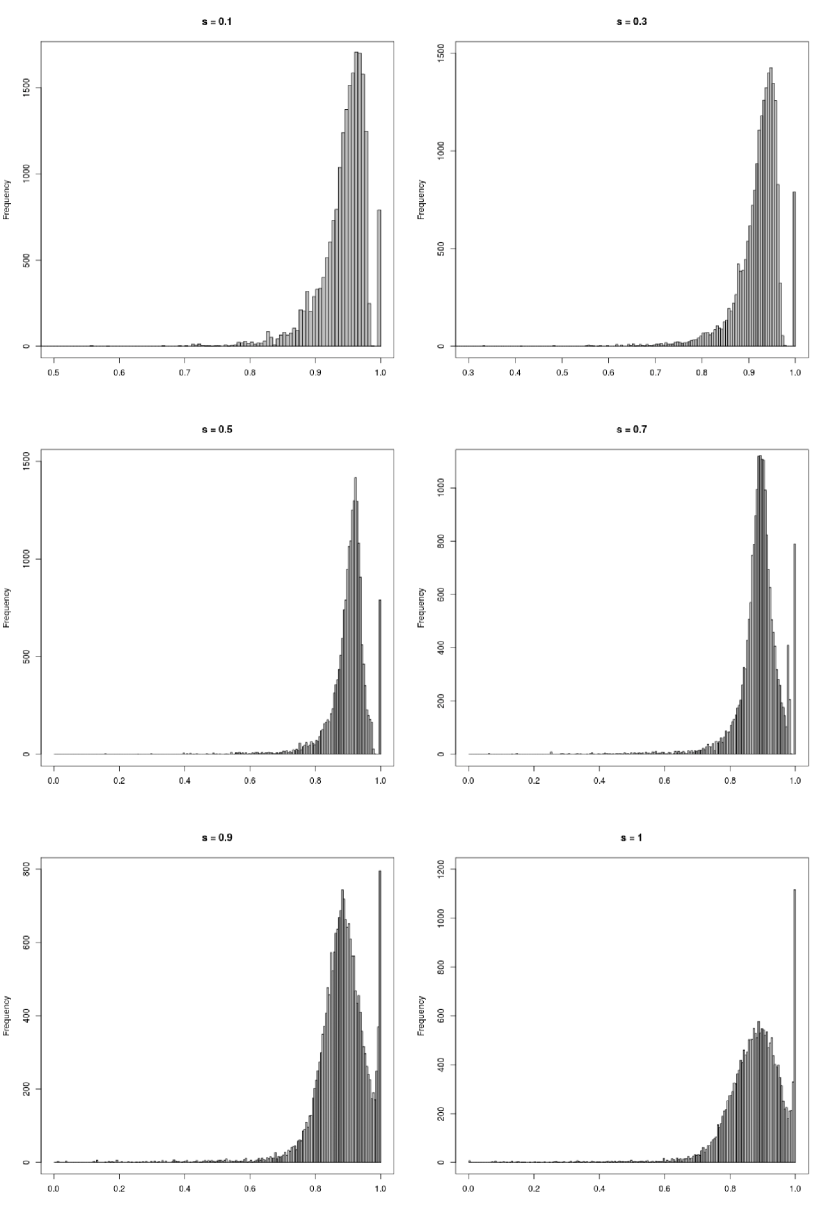
Figure 2: Histograms of Jaccard Entropy for family PF06850.

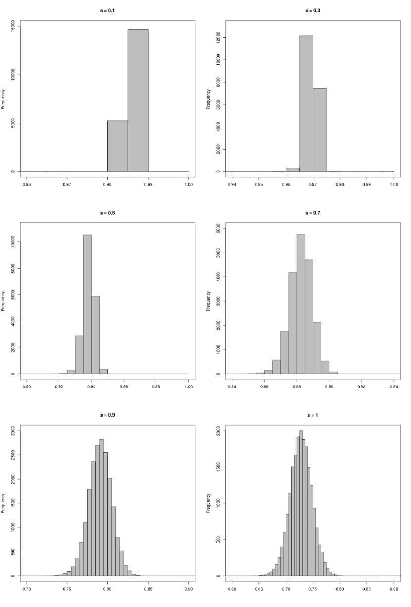
Figure 3: Histograms of Jaccard Entropy for family PF00135.

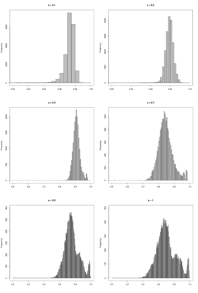
Figure 4: Histograms of Jaccard Entropy for family PF00005.

We also present the curves corresponding to the Average Jaccard Entropy Measure (formula) for 09 families, a well-posed measure, with the restriction $s\leq 1$, which is given by

$$J(s,f)=\frac{2}{n(n-1)}\sum_{j}\sum_{k}J_{jk}(s,f)$$

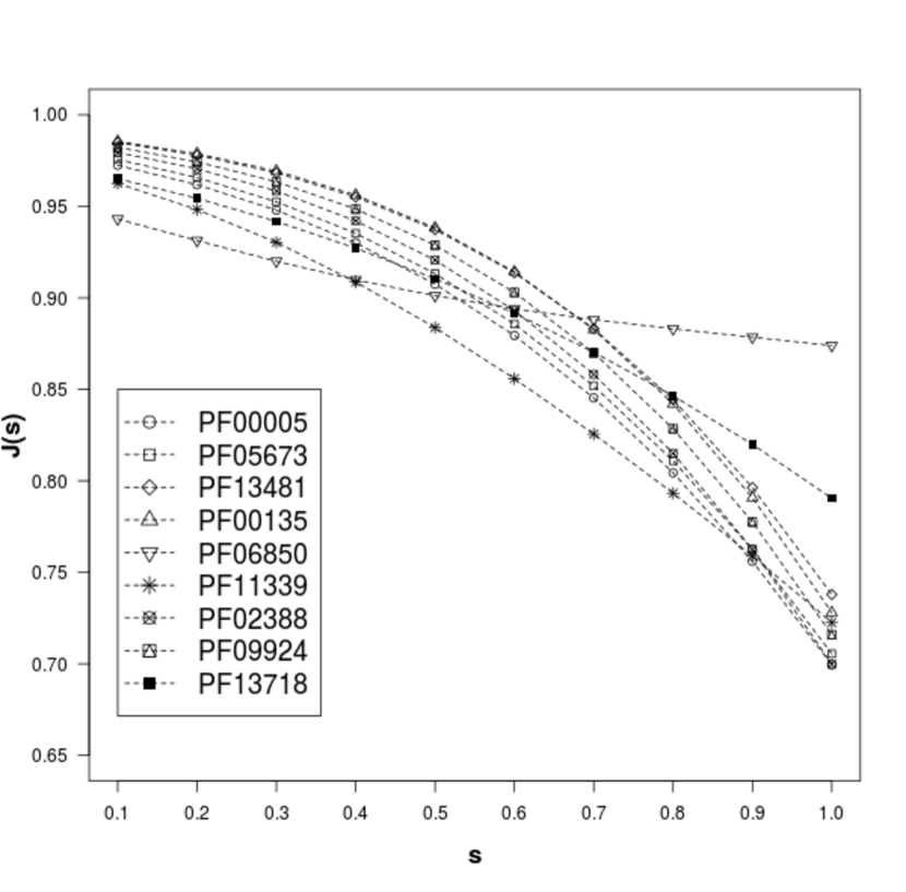
Figure 5: Curves of the Average Jaccard Entropy measures for families PF00005, PF05673, PF13481, PF00135, PF06850, PF11339, PF02388, PF09924, PF13718.

4 A First Assessment of Protein Databases with Entropy Measures

As a motivation for future research to be developed in sections 6, 7, we now introduce the first application of the formulae derived on the previous sections in terms of a naive analysis of averages and standard deviations of Entropy measure distributions. This will be also the first attempt at classifying the distribution of amino acids in a generic protein database. A robust approach to this research topic will be introduced and intensively analyzed on sections 6, 7 with the introduction of ANOVA statistics and the corresponding Hypothesis testing.

We then consider a Clan with F families. The Havrda-Charvat entropy measure associated to a pair of columns on the representative $m\times n$ array of each family with a specified value of the s parameter is given by

$$H_{jk}(s;f)=-\frac{1}{1-s}\left(1-\sum_{a}\sum_{b}\big{(}P_{jk}(a,b;f)\big{)}^{s}\right)$$ (54)

We can then define an average of these entropy measures for each family by

$$\langle H(s;f)\rangle=\frac{2}{n(n-1)}\sum_{j}\sum_{k}H_{jk}(s;f)$$ (55)

We also consider the average value of the averages over the set of F families:

$$\langle H(s)\rangle_{F}=\frac{1}{F}\sum_{f=1}^{F}\langle H(s;f)\rangle$$ (56)

The Standard deviation of the Entropy measures $H_{jk}(s;f)$ with relation to the given average in eq.(55) can be written as:

$$\sigma(s;f)=\left(\frac{1}{\frac{n(n-1)}{2}-1}\sum_{j}\sum_{k}\big{(}H_{jk}(s;f)-\langle H(s;f)\rangle\big{)}^{2}\right)^{1/2}$$ (57)

and finally, the Standard deviation of the average $\langle H(s;f)\rangle$ with respect to the average $\langle H(s)\rangle_{F}$:

$$\sigma_{F}(s)=\left(\frac{1}{F-1}\sum_{f=1}^{F}\big{(}\langle H(s;f)\rangle-\langle H(s)\rangle_{F}\big{)}^{2}\right)^{1/2}$$ (58)

We present in figs.6, 7 below the diagrams corresponding to formulae (55) and (57). We should stress that only Clans with a minimum of five families are considered.

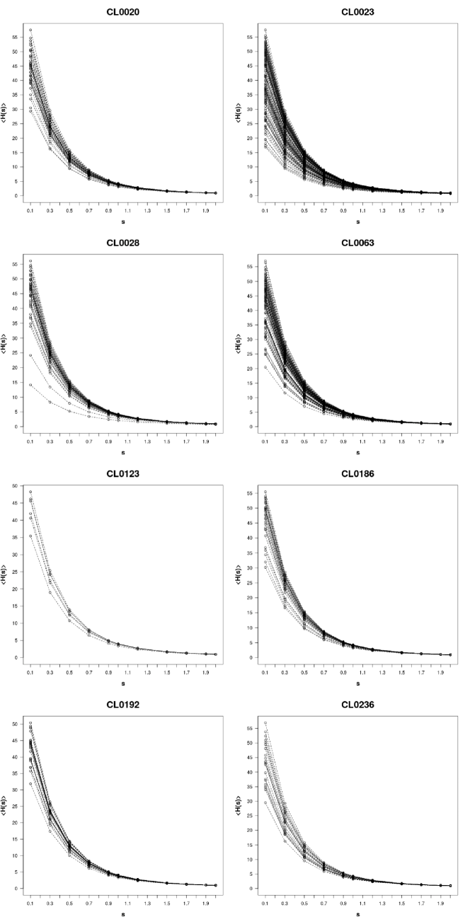
Figure 6: The Average values of the Havrda-Charvat Entropy measures for the families of a selected set of Clans and eleven values of the $s$-parameter, eq.(55).

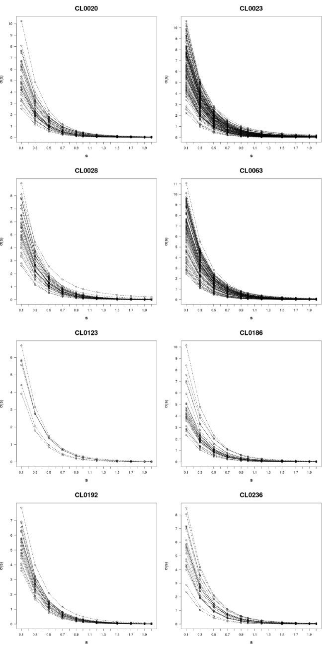
Figure 7: The standard deviation of the Havrda-Charvat Entropy measures with relation to the averages of these entropies for each family and eleven values of the $s$-parameter, eq.(57).

We now present the values of $\langle H(s)\rangle_{F}$ and $\sigma_{F}(s)$ for a selected number of Clans and eleven values of the $s$-parameter, according to eqs.(56) and (58).

Table 4: The average values and the standard deviation of the Average Havrda-Charvat Entropy measures for eleven values of the $s$-parameter and a selected set of 8 Clans.

Clans from Pfam 27.0 — Havrda-Charvat Entropies
Clan number	$\scriptstyle s$	$\scriptstyle\langle H(s)\rangle_{F}$	$\scriptstyle\sigma(s)_{F}$	Clan number	$\scriptstyle s$	$\scriptstyle\langle H(s)\rangle_{F}$	$\scriptstyle\sigma(s)_{F}$
	$\scriptstyle 0.1$	$\scriptstyle 44.212$	$\scriptstyle 6.396$		$\scriptstyle 0.1$	$\scriptstyle 43.001$	$\scriptstyle 4.667$
	$\scriptstyle 0.3$	$\scriptstyle 23.375$	$\scriptstyle 3.057$		$\scriptstyle 0.3$	$\scriptstyle 22.851$	$\scriptstyle 2.295$
	$\scriptstyle 0.5$	$\scriptstyle 12.992$	$\scriptstyle 1.492$		$\scriptstyle 0.5$	$\scriptstyle 12.765$	$\scriptstyle 1.161$
	$\scriptstyle 0.7$	$\scriptstyle 7.645$	$\scriptstyle 0.746$		$\scriptstyle 0.7$	$\scriptstyle 7.546$	$\scriptstyle 0.605$
	$\scriptstyle 0.9$	$\scriptstyle 4.784$	$\scriptstyle 0.384$		$\scriptstyle 0.9$	$\scriptstyle 4.741$	$\scriptstyle 0.326$
CL0020	$\scriptstyle 1.0$	$\scriptstyle 3.875$	$\scriptstyle 0.278$	CL0123	$\scriptstyle 1.0$	$\scriptstyle 3.846$	$\scriptstyle 0.242$
(38 families)	$\scriptstyle 1.2$	$\scriptstyle 2.661$	$\scriptstyle 0.150$	(06 families)	$\scriptstyle 1.2$	$\scriptstyle 2.648$	$\scriptstyle 0.137$
	$\scriptstyle 1.5$	$\scriptstyle 1.680$	$\scriptstyle 0.063$		$\scriptstyle 1.5$	$\scriptstyle 1.676$	$\scriptstyle 0.062$
	$\scriptstyle 1.7$	$\scriptstyle 1.311$	$\scriptstyle 0.038$		$\scriptstyle 1.7$	$\scriptstyle 1.309$	$\scriptstyle 0.038$
	$\scriptstyle 1.9$	$\scriptstyle 1.062$	$\scriptstyle 0.023$		$\scriptstyle 1.9$	$\scriptstyle 1.061$	$\scriptstyle 0.024$
	$\scriptstyle 2.0$	$\scriptstyle 0.967$	$\scriptstyle 0.018$		$\scriptstyle 2.0$	$\scriptstyle 0.966$	$\scriptstyle 0.019$
	$\scriptstyle 0.1$	$\scriptstyle 39.235$	$\scriptstyle 10.175$		$\scriptstyle 0.1$	$\scriptstyle 46.084$	$\scriptstyle 6.790$
	$\scriptstyle 0.3$	$\scriptstyle 20.908$	$\scriptstyle 4.984$		$\scriptstyle 0.3$	$\scriptstyle 24.260$	$\scriptstyle 3.224$
	$\scriptstyle 0.5$	$\scriptstyle 11.733$	$\scriptstyle 2.510$		$\scriptstyle 0.5$	$\scriptstyle 13.417$	$\scriptstyle 1.561$
	$\scriptstyle 0.7$	$\scriptstyle 6.982$	$\scriptstyle 1.305$		$\scriptstyle 0.7$	$\scriptstyle 7.853$	$\scriptstyle 0.772$
	$\scriptstyle 0.9$	$\scriptstyle 4.422$	$\scriptstyle 0.704$		$\scriptstyle 0.9$	$\scriptstyle 4.886$	$\scriptstyle 0.392$
CL0023	$\scriptstyle 1.0$	$\scriptstyle 3.604$	$\scriptstyle 0.525$	CL0186	$\scriptstyle 1.0$	$\scriptstyle 3.949$	$\scriptstyle 0.282$
(119 families)	$\scriptstyle 1.2$	$\scriptstyle 2.504$	$\scriptstyle 0.302$	(29 families)	$\scriptstyle 1.2$	$\scriptstyle 2.701$	$\scriptstyle 0.149$
	$\scriptstyle 1.5$	$\scriptstyle 1.606$	$\scriptstyle 0.144$		$\scriptstyle 1.5$	$\scriptstyle 1.696$	$\scriptstyle 0.060$
	$\scriptstyle 1.7$	$\scriptstyle 1.263$	$\scriptstyle 0.093$		$\scriptstyle 1.7$	$\scriptstyle 1.320$	$\scriptstyle 0.035$
	$\scriptstyle 1.9$	$\scriptstyle 1.030$	$\scriptstyle 0.063$		$\scriptstyle 1.9$	$\scriptstyle 1.067$	$\scriptstyle 0.020$
	$\scriptstyle 2.0$	$\scriptstyle 0.940$	$\scriptstyle 0.053$		$\scriptstyle 2.0$	$\scriptstyle 0.970$	$\scriptstyle 0.016$
	$\scriptstyle 0.1$	$\scriptstyle 44.906$	$\scriptstyle 7.996$		$\scriptstyle 0.1$	$\scriptstyle 42.862$	$\scriptstyle 4.566$
	$\scriptstyle 0.3$	$\scriptstyle 23.671$	$\scriptstyle 3.906$		$\scriptstyle 0.3$	$\scriptstyle 22.791$	$\scriptstyle 2.190$
	$\scriptstyle 0.5$	$\scriptstyle 13.114$	$\scriptstyle 1.961$		$\scriptstyle 0.5$	$\scriptstyle 12.741$	$\scriptstyle 1.072$
	$\scriptstyle 0.7$	$\scriptstyle 7.692$	$\scriptstyle 1.015$		$\scriptstyle 0.7$	$\scriptstyle 7.538$	$\scriptstyle 0.537$
	$\scriptstyle 0.9$	$\scriptstyle 4.799$	$\scriptstyle 0.545$		$\scriptstyle 0.9$	$\scriptstyle 4.739$	$\scriptstyle 0.275$
CL0028	$\scriptstyle 1.0$	$\scriptstyle 3.882$	$\scriptstyle 0.406$	CL0192	$\scriptstyle 1.0$	$\scriptstyle 3.847$	$\scriptstyle 0.199$
(41 families)	$\scriptstyle 1.2$	$\scriptstyle 2.660$	$\scriptstyle 0.232$	(26 families)	$\scriptstyle 1.2$	$\scriptstyle 2.650$	$\scriptstyle 0.107$
	$\scriptstyle 1.5$	$\scriptstyle 1.676$	$\scriptstyle 0.109$		$\scriptstyle 1.5$	$\scriptstyle 1.678$	$\scriptstyle 0.044$
	$\scriptstyle 1.7$	$\scriptstyle 1.307$	$\scriptstyle 0.070$		$\scriptstyle 1.7$	$\scriptstyle 1.311$	$\scriptstyle 0.026$
	$\scriptstyle 1.9$	$\scriptstyle 1.058$	$\scriptstyle 0.047$		$\scriptstyle 1.9$	$\scriptstyle 1.062$	$\scriptstyle 0.015$
	$\scriptstyle 2.0$	$\scriptstyle 0.963$	$\scriptstyle 0.039$		$\scriptstyle 2.0$	$\scriptstyle 0.967$	$\scriptstyle 0.012$
	$\scriptstyle 0.1$	$\scriptstyle 42.312$	$\scriptstyle 8.023$		$\scriptstyle 0.1$	$\scriptstyle 43.251$	$\scriptstyle 7.469$
	$\scriptstyle 0.3$	$\scriptstyle 22.454$	$\scriptstyle 3.857$		$\scriptstyle 0.3$	$\scriptstyle 22.905$	$\scriptstyle 3.564$
	$\scriptstyle 0.5$	$\scriptstyle 12.534$	$\scriptstyle 1.896$		$\scriptstyle 0.5$	$\scriptstyle 12.757$	$\scriptstyle 1.734$
	$\scriptstyle 0.7$	$\scriptstyle 7.411$	$\scriptstyle 0.956$		$\scriptstyle 0.7$	$\scriptstyle 7.524$	$\scriptstyle 0.863$
	$\scriptstyle 0.9$	$\scriptstyle 4.660$	$\scriptstyle 0.496$		$\scriptstyle 0.9$	$\scriptstyle 4.719$	$\scriptstyle 0.440$
CL0063	$\scriptstyle 1.0$	$\scriptstyle 3.784$	$\scriptstyle 0.362$	CL0236	$\scriptstyle 1.0$	$\scriptstyle 3.828$	$\scriptstyle 0.317$
(92 families)	$\scriptstyle 1.2$	$\scriptstyle 2.611$	$\scriptstyle 0.198$	(21 families)	$\scriptstyle 1.2$	$\scriptstyle 2.636$	$\scriptstyle 0.169$
	$\scriptstyle 1.5$	$\scriptstyle 1.658$	$\scriptstyle 0.086$		$\scriptstyle 1.5$	$\scriptstyle 1.669$	$\scriptstyle 0.069$
	$\scriptstyle 1.7$	$\scriptstyle 1.297$	$\scriptstyle 0.051$		$\scriptstyle 1.7$	$\scriptstyle 1.304$	$\scriptstyle 0.040$
	$\scriptstyle 1.9$	$\scriptstyle 1.053$	$\scriptstyle 0.032$		$\scriptstyle 1.9$	$\scriptstyle 1.058$	$\scriptstyle 0.024$
	$\scriptstyle 2.0$	$\scriptstyle 0.960$	$\scriptstyle 0.026$		$\scriptstyle 2.0$	$\scriptstyle 0.964$	$\scriptstyle 0.019$

In figs.8a and 8b below, we present the graphs corresponding to Table 4. These results just point out a more elaborate formulation of the problem.

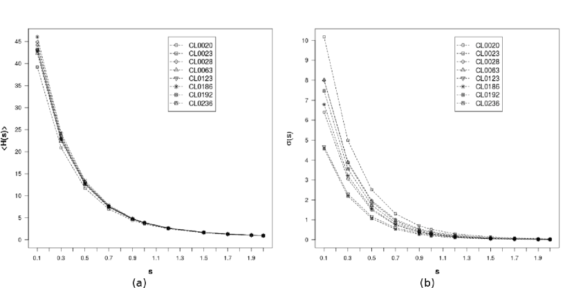
Figure 8: (a) The average values of Havrda-Charvat Entropies for a set of 08 Clans. (b) The Standard Deviation of the averages for Havrda-Charvat Entropies for a set of 08 Clans.

We now proceed to analyze a proposal (naive) for testing the robustness of the Clan concept. We will check if Pseudo-Clans which have the same number of families (a minimum of 05 families) of the corresponding Clans will have essentially different values of $\langle H(s)\rangle_{F}$ and $\sigma_{F}(s)$. The families to be associated with a Pseudo-Clan are obtained by sorting on the set of 1069 families and by withdrawal of the families already sorted. In Table 5 below we present the values $\langle H(s)\rangle_{F}$ and $\sigma_{F}(s)$ for the Pseudo-Clans obtained by the procedure described above.

The Figures 9a, 9b, do correspond to the comparison of data of Table 4 (Clans) with those of Table 5 (Pseudo-Clans). Clans are in red, Pseudo-Clans in blue.

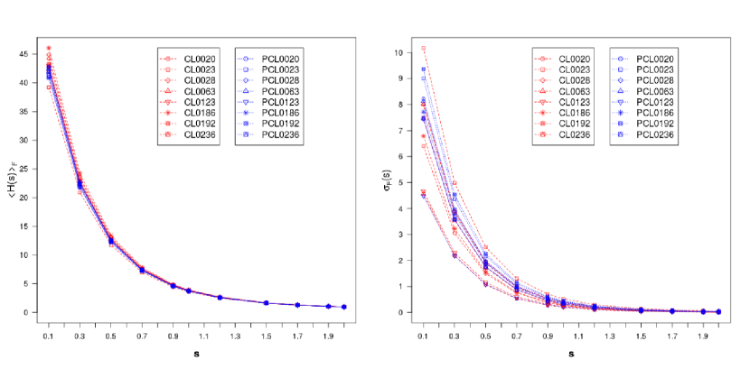
Figure 9: (a) The comparison of Clans and Pseudo-Clans average values. (b) The comparison of Clans and Pseudo-Clans standard deviation values.

Table 5: The average values and the standard deviation of the Average Havrda-Charvat Entropy measures for eleven values of the $s$-parameter and a selected set of 8 Pseudo-Clans.

Pseudo-Clans / Pfam 27.0 — Havrda-Charvat Entropies
Pseudo-Clan	$\scriptstyle s$	$\scriptstyle\langle H(s)\rangle_{F}$	$\scriptstyle\sigma(s)_{F}$		Pseudo-Clan	$\scriptstyle s$	$\scriptstyle\langle H(s)\rangle_{F}$	$\scriptstyle\sigma(s)_{F}$
number					number
	$\scriptstyle 0.1$	$\scriptstyle 42.381$	$\scriptstyle 8.224$			$\scriptstyle 0.1$	$\scriptstyle 42.042$	$\scriptstyle 4.484$
	$\scriptstyle 0.3$	$\scriptstyle 22.480$	$\scriptstyle 3.979$			$\scriptstyle 0.3$	$\scriptstyle 22.359$	$\scriptstyle 2.175$
	$\scriptstyle 0.5$	$\scriptstyle 12.542$	$\scriptstyle 1.972$			$\scriptstyle 0.5$	$\scriptstyle 12.508$	$\scriptstyle 1.082$
	$\scriptstyle 0.7$	$\scriptstyle 7.410$	$\scriptstyle 1.005$			$\scriptstyle 0.7$	$\scriptstyle 7.409$	$\scriptstyle 0.555$
	$\scriptstyle 0.9$	$\scriptstyle 4.657$	$\scriptstyle 0.528$			$\scriptstyle 0.9$	$\scriptstyle 4.667$	$\scriptstyle 0.293$
PCL0020	$\scriptstyle 1.0$	$\scriptstyle 3.781$	$\scriptstyle 0.389$		PCL0123	$\scriptstyle 1.0$	$\scriptstyle 3.791$	$\scriptstyle 0.216$
(38 families)	$\scriptstyle 1.2$	$\scriptstyle 2.607$	$\scriptstyle 0.216$		(06 families)	$\scriptstyle 1.2$	$\scriptstyle 2.618$	$\scriptstyle 0.120$
	$\scriptstyle 1.5$	$\scriptstyle 1.655$	$\scriptstyle 0.096$			$\scriptstyle 1.5$	$\scriptstyle 1.663$	$\scriptstyle 0.053$
	$\scriptstyle 1.7$	$\scriptstyle 1.295$	$\scriptstyle 0.059$			$\scriptstyle 1.7$	$\scriptstyle 1.301$	$\scriptstyle 0.032$
	$\scriptstyle 1.9$	$\scriptstyle 1.051$	$\scriptstyle 0.037$			$\scriptstyle 1.9$	$\scriptstyle 1.056$	$\scriptstyle 0.020$
	$\scriptstyle 2.0$	$\scriptstyle 0.958$	$\scriptstyle 0.030$			$\scriptstyle 2.0$	$\scriptstyle 0.962$	$\scriptstyle 0.016$
	$\scriptstyle 0.1$	$\scriptstyle 41.023$	$\scriptstyle 9.007$			$\scriptstyle 0.1$	$\scriptstyle 40.888$	$\scriptstyle 7.719$
	$\scriptstyle 0.3$	$\scriptstyle 21.825$	$\scriptstyle 4.360$			$\scriptstyle 0.3$	$\scriptstyle 21.790$	$\scriptstyle 3.768$
	$\scriptstyle 0.5$	$\scriptstyle 12.219$	$\scriptstyle 2.163$			$\scriptstyle 0.5$	$\scriptstyle 12.220$	$\scriptstyle 1.891$
	$\scriptstyle 0.7$	$\scriptstyle 7.247$	$\scriptstyle 1.104$			$\scriptstyle 0.7$	$\scriptstyle 7.258$	$\scriptstyle 0.981$
	$\scriptstyle 0.9$	$\scriptstyle 4.573$	$\scriptstyle 0.582$			$\scriptstyle 0.9$	$\scriptstyle 4.585$	$\scriptstyle 0.529$
PCL0023	$\scriptstyle 1.0$	$\scriptstyle 3.714$	$\scriptstyle 0.427$		PCL0186	$\scriptstyle 1.0$	$\scriptstyle 3.730$	$\scriptstyle 0.394$
(119 families)	$\scriptstyle 1.2$	$\scriptstyle 2.573$	$\scriptstyle 0.240$		(29 families)	$\scriptstyle 1.2$	$\scriptstyle 2.582$	$\scriptstyle 0.227$
	$\scriptstyle 1.5$	$\scriptstyle 1.640$	$\scriptstyle 0.109$			$\scriptstyle 1.5$	$\scriptstyle 1.646$	$\scriptstyle 0.109$
	$\scriptstyle 1.7$	$\scriptstyle 1.286$	$\scriptstyle 0.068$			$\scriptstyle 1.7$	$\scriptstyle 1.290$	$\scriptstyle 0.071$
	$\scriptstyle 1.9$	$\scriptstyle 1.046$	$\scriptstyle 0.044$			$\scriptstyle 1.9$	$\scriptstyle 1.048$	$\scriptstyle 0.049$
	$\scriptstyle 2.0$	$\scriptstyle 0.954$	$\scriptstyle 0.037$			$\scriptstyle 2.0$	$\scriptstyle 0.956$	$\scriptstyle 0.041$
	$\scriptstyle 0.1$	$\scriptstyle 42.716$	$\scriptstyle 7.435$			$\scriptstyle 0.1$	$\scriptstyle 42.756$	$\scriptstyle 9.361$
	$\scriptstyle 0.3$	$\scriptstyle 23.658$	$\scriptstyle 3.573$			$\scriptstyle 0.3$	$\scriptstyle 22.666$	$\scriptstyle 4.535$
	$\scriptstyle 0.5$	$\scriptstyle 12.641$	$\scriptstyle 1.756$			$\scriptstyle 0.5$	$\scriptstyle 12.635$	$\scriptstyle 2.253$
	$\scriptstyle 0.7$	$\scriptstyle 7.468$	$\scriptstyle 0.886$			$\scriptstyle 0.7$	$\scriptstyle 7.458$	$\scriptstyle 1.151$
	$\scriptstyle 0.9$	$\scriptstyle 4.692$	$\scriptstyle 0.460$			$\scriptstyle 0.9$	$\scriptstyle 4.681$	$\scriptstyle 0.608$
PCL0028	$\scriptstyle 1.0$	$\scriptstyle 3.808$	$\scriptstyle 0.335$		PCL0192	$\scriptstyle 1.0$	$\scriptstyle 3.797$	$\scriptstyle 0.448$
(41 families)	$\scriptstyle 1.2$	$\scriptstyle 2.625$	$\scriptstyle 0.183$		(26 families)	$\scriptstyle 1.2$	$\scriptstyle 2.615$	$\scriptstyle 0.250$
	$\scriptstyle 1.5$	$\scriptstyle 1.664$	$\scriptstyle 0.079$			$\scriptstyle 1.5$	$\scriptstyle 1.657$	$\scriptstyle 0.113$
	$\scriptstyle 1.7$	$\scriptstyle 1.302$	$\scriptstyle 0.048$			$\scriptstyle 1.7$	$\scriptstyle 1.296$	$\scriptstyle 0.070$
	$\scriptstyle 1.9$	$\scriptstyle 1.056$	$\scriptstyle 0.030$			$\scriptstyle 1.9$	$\scriptstyle 1.051$	$\scriptstyle 0.046$
	$\scriptstyle 2.0$	$\scriptstyle 0.962$	$\scriptstyle 0.024$			$\scriptstyle 2.0$	$\scriptstyle 0.958$	$\scriptstyle 0.037$
	$\scriptstyle 0.1$	$\scriptstyle 41.870$	$\scriptstyle 8.134$			$\scriptstyle 0.1$	$\scriptstyle 41.551$	$\scriptstyle 7.476$
	$\scriptstyle 0.3$	$\scriptstyle 22.252$	$\scriptstyle 3.914$			$\scriptstyle 0.3$	$\scriptstyle 22.090$	$\scriptstyle 3.591$
	$\scriptstyle 0.5$	$\scriptstyle 12.440$	$\scriptstyle 1.929$			$\scriptstyle 0.5$	$\scriptstyle 12.357$	$\scriptstyle 1.763$
	$\scriptstyle 0.7$	$\scriptstyle 7.366$	$\scriptstyle 0.977$			$\scriptstyle 0.7$	$\scriptstyle 7.322$	$\scriptstyle 0.887$
	$\scriptstyle 0.9$	$\scriptstyle 4.638$	$\scriptstyle 0.510$			$\scriptstyle 0.9$	$\scriptstyle 4.614$	$\scriptstyle 0.459$
PCL0063	$\scriptstyle 1.0$	$\scriptstyle 3.771$	$\scriptstyle 0.375$		PCL0236	$\scriptstyle 1.0$	$\scriptstyle 3.752$	$\scriptstyle 0.334$
(92 families)	$\scriptstyle 1.2$	$\scriptstyle 2.603$	$\scriptstyle 0.207$		(21 families)	$\scriptstyle 1.2$	$\scriptstyle 2.595$	$\scriptstyle 0.181$
	$\scriptstyle 1.5$	$\scriptstyle 1.654$	$\scriptstyle 0.092$			$\scriptstyle 1.5$	$\scriptstyle 1.652$	$\scriptstyle 0.077$
	$\scriptstyle 1.7$	$\scriptstyle 1.295$	$\scriptstyle 0.057$			$\scriptstyle 1.7$	$\scriptstyle 1.294$	$\scriptstyle 0.046$
	$\scriptstyle 1.9$	$\scriptstyle 1.052$	$\scriptstyle 0.036$			$\scriptstyle 1.9$	$\scriptstyle 1.051$	$\scriptstyle 0.028$
	$\scriptstyle 2.0$	$\scriptstyle 0.959$	$\scriptstyle 0.030$			$\scriptstyle 2.0$	$\scriptstyle 0.959$	$\scriptstyle 0.022$

From the figures and tables above we can see that the region $s\leq 1$ leads to a better characterization of the Entropy measures distributions on protein databases.

For completeness, we list some useful formulae obtained from eqs.(55), (56), (58) which help to predict the profile of the curves above:

$$\langle H(s;f)\rangle=-\frac{1}{1-s}\left(1-\frac{2}{n(n-1)}\sum_{a,b,j,k}e^{-s\lvert\log P_{jk}(a,b;f)\rvert}\right)$$ (59)

$$\langle H(s)\rangle_{F}=-\frac{1}{1-s}\left(1-\frac{2}{Fn(n-1)}\sum_{f,a,b,j,k}e^{-s\lvert\log P_{jk}(a,b;f)\rvert}\right)$$ (60)

$$\sigma_{F}(s)=\frac{2(F-1)^{1/2}}{Fn(n-1)}\left(\sum_{f=1}^{F}\left(\sum_{a,b,j,k}e^{-s\lvert\log P_{jk}(a,b;f)\rvert}\right)^{2}\right)^{1/2}$$ (61)

5 The treatment of data with the Maple Computing system and its inadequacy for calculating Joint probabilities of occurrence. Alternative systems.

In this section, we specifically study the performance of the Maple system and an example of alternative computing system, the Perl system, for calculating the simple and joint probabilities of occurrences of amino acids. We also use these two systems for calculating 19 $s$-power values of these probabilities. We now select the family PF06850 in order to get an idea of the CPU and real times which are necessary for calculating the probabilities and their powers for the set of 1069 families. We start the calculation by adopting the Maple system version 18. There are some comments to be made on the construction of a computational code for calculating joint probabilities. This will be done in detail at the end of CPU and real times for the calculation of the simple and joint probabilities by using the developed code. The table below will repeat the times for calculating $200\times 20=4\times 10^{3}$ and $200\times\frac{200-1}{2}\times 20\times 20=7.96\times 10^{6}$ of simple and joint probability values, respectively, for the PF06850 Pfam family.

Table 6: CPU time and real times for the calculation of the simple and joint probabilities of occurrence associated with the protein family PF06850.

Maple System, version 18	$t_{CPU}$ (sec)	$t_{R}$ (sec)
Simple probabilities	$0.527$	$0.530$
Joint probabilities	$5073.049$	$4650.697$

After calculating all values of the probabilities $p_{j}(a)$ and $P_{jk}(a,b)$, we can proceed to evaluate the powers $\big{(}p_{j}(a)\big{)}^{s}$ and $\big{(}P_{j}k(a,b)\big{)}^{s}$ for 19 $s$-values. Our aim will be to use these values for calculating the Entropy Measures according to eqs.(32), (33). It should be noticed that the values of $p_{j}(a)$ and $P_{jk}(a,b)$, have to be calculated only once by using a specific computational code already referred on this work. Nevertheless, the use of the code for calculating the joint probabilities associated to 1069 protein families is the hardest of all calculations to be undertaken and it takes too much time. These probabilities once calculated should be grouped in sets of 400 values each corresponding to a pair of columns $j$, $k$ among the $\frac{n(n-1)}{2}$ feasible ones and the calculating of entropy value associated to this pair of columns $j$, $k$. Given a $s$-value and after calculating the entropy of this first pair $H_{1\,2}$ as a function of the 400 variables $\big{(}P_{jk}(a,b)\big{)}^{s}$, $j\neq 1$, $k\neq 2$ and he/she will proceeds to calculate again all values of $\frac{n(n-1)}{2}\times(20)^{2}$ in order to extract another value of joint probability for calculating the corresponding entropy value. This seems to be associated to the unknowing of the concepts of a function of several variables, unfortunately. After circumventing these mistakes coming from a bad educational formation, we succeed at keeping all calculated values of the probabilities and we then proceed to the calculation of the powers $\big{(}p_{j}(a)\big{)}^{s}$, $\big{(}P_{jk}(a,b)\big{)}^{s}$ of these values and the corresponding entropy measures. In tables 7, 8, 9, 10 below, we report all these calculations for 19 values of the $s$-parameter.

Table 7: CPU and real times for the calculation of 19 $s$-powers of simple probabilities of occurrence associated with the protein family PF06850.

Maple System, version 18,
$s$-powers of probability $\big{(}p_{j}(a)\big{)}^{s}$
$s$	$t_{CPU}$ (sec)	$t_{R}$ (sec)
$0.1$	$0.263$	$0.358$
$0.2$	$0.137$	$0.145$
$0.3$	$0.268$	$0.277$
$0.4$	$0.139$	$0.153$
$0.5$	$0.240$	$0.219$
$0.6$	$0.144$	$0.157$
$0.7$	$0.276$	$0.254$
$0.8$	$0.144$	$0.157$
$0.9$	$0.264$	$0.235$
$1.0$	$0.088$/$0.151$	$0.095$/$0.307$
$2.0$	$0.153$	$0.095$
$3.0$	$0.128$	$0.131$
$4.0$	$0.148$	$0.141$
$5.0$	$0.096$	$0.144$
$6.0$	$0.148$	$0.167$
$7.0$	$0.148$	$0.155$
$8.0$	$0.181$	$0.094$
$9.0$	$0.104$	$0.092$
$10.0$	$0.104$	$0.100$
Total	$3.173$	$3.164$

Table 8: CPU and real times for the calculation of 19 $s$-powers of joint probabilities of occurrence associated with the protein family PF06850.

Maple System, version 18,
$s$-powers of probability $\big{(}P_{jk}(a,b)\big{)}^{s}$
$s$	$t_{CPU}$ (sec)	$t_{R}$ (sec)
$0.1$	$390.432$	$206.646$
$0.2$	$382.887$	$202.282$
$0.3$	$401.269$	$210.791$
$0.4$	$416.168$	$216.993$
$0.5$	$427.572$	$221.541$
$0.6$	$430.604$	$223.227$
$0.7$	$421.904$	$218.484$
$0.8$	$434.888$	$224.267$
$0.9$	$431.948$	$223.023$
$1.0$	$442.933$/$482.612$	$224.731$/$259.301$
$2.0$	$176.212$	$147.455$
$3.0$	$234.100$	$174.853$
$4.0$	$289.184$	$181.552$
$5.0$	$327.740$	$178.117$
$6.0$	$334.800$	$194.691$
$7.0$	$349.064$	$195.258$
$8.0$	$361.304$	$195.437$
$9.0$	$386.217$	$197.150$
$10.0$	$397.276$	$197.868$
Total	$7036.502$	$3834.366$

The last row in tables 7, 8, includes the times necessary for calculating the probabilities of table 6.

We are then able to proceed to the calculation of the corresponding Havrda-Charvat entropy measures, $H_{j}(s)$, $H_{jk}(s)$: The results for 19 $s$-values are given in tables 9, 10 below.

Table 9: CPU and real times for the calculation of the Entropy measures $H_{j}(s)$ for the protein family PF06850.

Maple System, version 18,
Entropy Measures $H_{j}(s)$
$s$	$t_{CPU}$ (sec)	$t_{R}$ (sec)
$0.1$	$0.148$	$0.261$
$0.2$	$0.084$	$0.153$
$0.3$	$0.120$	$0.189$
$0.4$	$0.124$	$0.198$
$0.5$	$0.160$	$0.299$
$0.6$	$0.092$	$0.139$
$0.7$	$0.159$	$0.199$
$0.8$	$0.137$	$0.175$
$0.9$	$0.120$	$0.166$
$1.0$	$0.192$/$0.175$	$0.339$/$0.159$
$2.0$	$0.144$	$0.099$
$3.0$	$0.147$	$0.105$
$4.0$	$0.084$	$0.101$
$5.0$	$0.136$	$0.070$
$6.0$	$0.096$	$0.119$
$7.0$	$0.115$	$0.078$
$8.0$	$0.120$	$0.109$
$9.0$	$0.133$	$0.080$
$10.0$	$0.132$	$0.133$
Total	$2.443$	$3.012$

Table 10: CPU and real times for the calculation of the Entropy measures $H_{jk}(s)$ for the protein family PF06850.

Maple System, version 18,
Entropy Measures $H_{jk}(s)$
$s$	$t_{CPU}$ (sec)	$t_{R}$ (sec)
$0.1$	$156.332$	$133.242$
$0.2$	$160.797$	$136.706$
$0.3$	$169.024$	$140.960$
$0.4$	$176.824$	$147.853$
$0.5$	$184.120$	$150.163$
$0.6$	$190.304$	$154.058$
$0.7$	$196.633$	$157.750$
$0.8$	$205.940$	$164.101$
$0.9$	$215.559$	$169.549$
$1.0$	$253.648$/$124.501$	$204.634$/$148.993$
$2.0$	$141.148$	$184.030$
$3.0$	$158.536$	$167.173$
$4.0$	$173.136$	$181.282$
$5.0$	$197.680$	$238.723$
$6.0$	$215.000$	$111.476$
$7.0$	$145.257$	$115.221$
$8.0$	$156.848$	$122.957$
$9.0$	$157.300$	$126.233$
$10.0$	$166.399$	$135.080$
Total	$3420.485$	$2941.791$

The total time for calculating all the Havrda-Charvat Entropy measure content of probabilities of occurrence of amino acids on a specific family is given in table 11 below.

Table 11: Total CPU and real times for calculating the Entropy measure content of a family PF06850 and approximations for Grand Total of all sample space.

Maple System,	Entropy Measures	Entropy Measures
version 18	$\scriptstyle H\!_{j}(s)$ — 19 $\scriptstyle s$-values	$\scriptstyle H\!_{jk}(s)$ — 19 $\scriptstyle s$-values
Total CPU time	$\scriptstyle 0.527+3.173+2.443$	$\scriptstyle 5,073.049+7,036.502+$
(family PF06850)	$\scriptstyle=6.143$ sec	$\scriptstyle 3,420.485=15,530.036$ sec
Grand Total CPU time	$\scriptstyle 6,566.867$ sec	$\scriptstyle 16,601,608.484$ sec
(1069 families)	$\scriptstyle=1.824$ hs	$\scriptstyle=192.148$ days
Total Real time	$\scriptstyle 0.530+3.164+3.012$	$\scriptstyle 4,650.697+3,834.366+$
(family PF06850)	$\scriptstyle=6.706$ sec	$\scriptstyle 2,941.791=11,426.854$ sec
Grand Total Real time	$\scriptstyle 7,168.714$ sec	$\scriptstyle 12,215,306.926$ sec
(1069 families)	$\scriptstyle=1.991$ hs	$\scriptstyle=141.381$ days

From inspections of table 11, we realize that the Total CPU and real times for calculating the Havrda-Charvat entropies $H_{j}(s)$, of simple probabilities of occurrence $p_{j}(a)$ are obtained by summing up the total time results from tables 6, 7 and 9. For the Havrda-Charvat entropies $H_{jk}(s)$, we have to sum up the total times at table 6, 8 and 10. We take for granted that the times for calculating the Entropy Measure content of each family will not differ too much and the results 3rd and 5th rows of table 11 are obtained by multiplying by 1069 — the number of families in the sample space.

The results of table 11 suggest the inadequacy of the Maple computing system for analyzing the Entropy measure content of an example of protein database. We have restricted ourselves to operate with usual operating systems, Linux or OSX, on laptops. We have also worked with the alternative Perl computing system. The Maple computing system has an “array” structure which is very effective for doing calculations which require a knowledge of mathematical methods. On the contrary, the alternative Perl computing system has a “hash” structure as was emphasized in the 2nd section and it operates very well elementary operations with very large numbers. It is essential the comparison of a senior erudite which is largely conversant with a large amount of mathematical methods versus a “genius” brought to fame by media, who is able only to multiply in a very fast way, numbers of many digits.

In order to specify the probabilities of computational configurations with the usual desktops and laptops, we list below some of them which have been used in the present work. The computing systems were the Maple ($M$) and Perl ($P$), the operating systems, the Linux ($L$) and Mac OSX ($O$) and the structures: The Array I ($A_{I}$), Array II ($A_{I\!I}$) and Hash ($H$) (page 8, section 2). The available computational configurations to undertake the task of assessment of protein databases with Entropy measures could be listed as:

1. $MLA_{I}$ — Maple, Linux, Array I

2. $POH$ — Perl, OSX, Hash

3. $PLA_{I\!I}$ — Perl, Linux, Array II

4. $POA_{I\!I}$ — Perl, OSX, Array II

The following table will display a comparison of the CPU and real times for the calculation of 19 $s$-values of the joint probabilities $\big{(}P_{jk}(a,b)^{s}\big{)}$ for the protein family PF06850 by the four configurations nominated above. It should be stressed that we are here comparing the times for calculating the $s$-power with the values of the probabilities themselves previously calculated and kept on a file.

Table 12: A comparison of calculation times (CPU and real) for 19 $s$-powers of joint probabilities only of PF06850 protein family, using the four configurations $MLA_{I}$, $POA_{I\!I}$, $PLA_{I\!I}$, $POH$.

$\scriptstyle\mathbf{s}$	$\scriptstyle\mathbf{t_{CPU}}$ (sec)				$\scriptstyle\mathbf{t_{R}}$ (sec)
	$\scriptstyle MLA_{I}$	$\scriptstyle POA_{I\!I}$	$\scriptstyle PLA_{I\!I}$	$\scriptstyle POH$	$\scriptstyle MLA_{I}$	$\scriptstyle POA_{I\!I}$	$\scriptstyle PLA_{I\!I}$	$\scriptstyle POH$
$\scriptstyle 0.1$	$\scriptstyle 390.432$	$\scriptstyle 33.478$	$\scriptstyle\mathbf{41.633}$	$\scriptstyle 24.849$	$\scriptstyle 206.646$	$\scriptstyle 88.527$	$\scriptstyle 83.139$	$\scriptstyle 26.862$
$\scriptstyle 0.2$	$\scriptstyle 382.887$	$\scriptstyle 31.711$	$\scriptstyle 26.483$	$\scriptstyle 25.093$	$\scriptstyle 202.282$	$\scriptstyle 80.624$	$\scriptstyle 53.384$	$\scriptstyle 26.904$
$\scriptstyle 0.3$	$\scriptstyle 401.269$	$\scriptstyle 31.726$	$\scriptstyle 25.286$	$\scriptstyle 24.751$	$\scriptstyle 210.791$	$\scriptstyle 80.519$	$\scriptstyle 50.689$	$\scriptstyle 27.305$
$\scriptstyle 0.4$	$\scriptstyle 416.168$	$\scriptstyle 31.448$	$\scriptstyle 26.138$	$\scriptstyle 26.345$	$\scriptstyle 216.993$	$\scriptstyle 79.032$	$\scriptstyle 51.409$	$\scriptstyle 27.687$
$\scriptstyle 0.5$	$\scriptstyle 427.572$	$\scriptstyle 32.860$	$\scriptstyle\mathbf{25.822}$	$\scriptstyle 26.726$	$\scriptstyle 221.541$	$\scriptstyle 93.048$	$\scriptstyle 51.334$	$\scriptstyle 27.528$
$\scriptstyle 0.6$	$\scriptstyle 430.604$	$\scriptstyle 33.444$	$\scriptstyle 27.013$	$\scriptstyle 25.021$	$\scriptstyle 223.227$	$\scriptstyle 102.317$	$\scriptstyle 52.889$	$\scriptstyle 25.408$
$\scriptstyle 0.7$	$\scriptstyle 421.904$	$\scriptstyle 31.053$	$\scriptstyle 25.814$	$\scriptstyle 25.011$	$\scriptstyle 218.484$	$\scriptstyle 79.255$	$\scriptstyle 51.466$	$\scriptstyle 26.414$
$\scriptstyle 0.8$	$\scriptstyle 434.888$	$\scriptstyle 31.526$	$\scriptstyle 26.725$	$\scriptstyle 25.183$	$\scriptstyle 224.267$	$\scriptstyle 80.469$	$\scriptstyle 53.388$	$\scriptstyle 25.668$
$\scriptstyle 0.9$	$\scriptstyle 431.948$	$\scriptstyle 31.482$	$\scriptstyle 26.895$	$\scriptstyle 25.409$	$\scriptstyle 223.023$	$\scriptstyle 80.002$	$\scriptstyle 53.579$	$\scriptstyle 25.536$
$\scriptstyle 1.0$	$\scriptstyle 442.933$	$\scriptstyle 32.056$	$\scriptstyle 25.990$	$\scriptstyle 25.096$	$\scriptstyle 224.731$	$\scriptstyle 80.917$	$\scriptstyle 51.687$	$\scriptstyle 25.640$
$\scriptstyle 2.0$	$\scriptstyle 176.212$	$\scriptstyle 32.638$	$\scriptstyle 27.089$	$\scriptstyle 26.012$	$\scriptstyle 147.454$	$\scriptstyle 80.751$	$\scriptstyle 54.384$	$\scriptstyle 26.960$
$\scriptstyle 3.0$	$\scriptstyle 234.100$	$\scriptstyle 31.892$	$\scriptstyle 25.766$	$\scriptstyle 24.498$	$\scriptstyle 174.853$	$\scriptstyle 85.853$	$\scriptstyle 51.843$	$\scriptstyle 24.717$
$\scriptstyle 4.0$	$\scriptstyle 284.184$	$\scriptstyle 31.662$	$\scriptstyle 26.515$	$\scriptstyle 25.251$	$\scriptstyle 181.552$	$\scriptstyle 91.837$	$\scriptstyle 52.636$	$\scriptstyle 25.718$
$\scriptstyle 5.0$	$\scriptstyle 327.740$	$\scriptstyle 32.295$	$\scriptstyle 27.516$	$\scriptstyle 24.925$	$\scriptstyle 178.117$	$\scriptstyle 87.486$	$\scriptstyle 54.908$	$\scriptstyle 25.814$
$\scriptstyle 6.0$	$\scriptstyle 334.800$	$\scriptstyle 32.674$	$\scriptstyle 28.126$	$\scriptstyle 25.440$	$\scriptstyle 194.691$	$\scriptstyle 86.569$	$\scriptstyle 54.611$	$\scriptstyle 25.847$
$\scriptstyle 7.0$	$\scriptstyle 349.064$	$\scriptstyle 31.674$	$\scriptstyle 23.908$	$\scriptstyle 26.389$	$\scriptstyle 195.258$	$\scriptstyle 86.215$	$\scriptstyle 49.262$	$\scriptstyle 27.745$
$\scriptstyle 8.0$	$\scriptstyle 361.304$	$\scriptstyle 33.105$	$\scriptstyle 26.020$	$\scriptstyle 25.106$	$\scriptstyle 195.437$	$\scriptstyle 116.601$	$\scriptstyle 51.889$	$\scriptstyle 26.735$
$\scriptstyle 9.0$	$\scriptstyle 386.217$	$\scriptstyle 31.881$	$\scriptstyle 26.208$	$\scriptstyle 24.783$	$\scriptstyle 197.150$	$\scriptstyle 81.372$	$\scriptstyle 53.114$	$\scriptstyle 25.155$
$\scriptstyle 10.0$	$\scriptstyle 397.276$	$\scriptstyle 32.269$	$\scriptstyle 26.125$	$\scriptstyle 24.979$	$\scriptstyle 197.868$	$\scriptstyle 87.963$	$\scriptstyle 52.541$	$\scriptstyle 26.504$
Total	$\scriptstyle 7036.502$	$\scriptstyle 611.374$	$\scriptstyle 515.072$	$\scriptstyle 480.867$	$\scriptstyle 3834.365$	$\scriptstyle 1649.357$	$\scriptstyle 1028.655$	$\scriptstyle 500.147$
Total	$\scriptstyle 7,522,020.640$	$\scriptstyle 653,588.806$	$\scriptstyle 550,611.968$	$\scriptstyle 514,046.813$	$\scriptstyle 4,098,936.190$	$\scriptstyle 1,763,162.630$	$\scriptstyle 1,099,632.200$	$\scriptstyle 534,157.143$
(1069) families	$\scriptstyle=87.067$ days	$\scriptstyle=7.565$ days	$\scriptstyle=6.373$ days	$\scriptstyle=5.950$ days	$\scriptstyle=47.441$ days	$\scriptstyle=20.407$ days	$\scriptstyle=12.727$ days	$\scriptstyle=6.188$ days

We can check that the times on table 12 seem to be generically ordered as

$$t_{MLA_{I}}>t_{POA_{I\!I}}>t_{PLA_{I\!I}}>t_{POH}$$ (62)

From this ordering of computing times, we are then able to consider that the inconvenience of using the “hash” structure which has been emphasized on section 2, was not circumvented by working with a modified array structure ($A_{I\!I}$ instead of $H$), at least for the Mac Pro machine used in these calculations. We do not also know if this machine has been even used with an “overload” of programs from the assumed part-time job of the experimenter (maybe 99.99% time job!). Anyhow, the usual Hash structure of Perl computing system has delayed the calculation of the Entropy Measures and even with the help of the modified $A_{I\!I}$ structure, it does not succeed at computing with this structure if operated on a OSX computing system.

On the other hand, the configuration $MLA_{I}$ could be chosen for parallelizing the respective adopted code in a work to be done with supercomputer facilities. If we try to avoid this kind of computational facility, in the belief that the problem of classifying the distribution of amino acids of a protein database in terms of Entropy Measures could be treated with less powerful but very objective “weapons”, we should try to look for very fast laptop machines instead, by working with a Linux operating system, a Perl computing system and a modified array structure. This means that it would be worthwhile the continuation of the present work with the $PLA_{I\!I}$ configuration. This is now in progress and will be published elsewhere.

We summarize the conclusions commented above on tables 13–16 below for the calculation of CPU and Real times of 19 $s$-powers of joint probabilities $\big{(}P_{jk}(a,b)\big{)}^{s}$ and the corresponding values of Havrda-Charvat entropy measures. The necessary times for calculating the joint probabilities themselves has not been taken into consideration. It would be very useful to make a comparison of the results of table 10 with those on tables 14, 16, and table 12 with tables 13, 15 as well.

As a last remark of this section, we shall take into consideration, the restrictions of $s\leq 1$ for working with Jaccard Entropy measures and we calculate the total CPU and real times for the set of $s$-values: $s=$ $0.1$, $0.2$, $0.3$, $0.4$, $0.5$, $0.6$, $0.7$, $0.8$, $0.9$, $1.0$. The results are presented in table 17 below for the $PLA_{I\!I}$ configuration and the calculation of the Havrda-Charvat entropies.

Table 13: Calculation of CPU and Real times of 19 $s$-powers of joint probabilities $\big{(}P_{jk}(a,b)\big{)}^{s}$ measures for 06 families from 03 Clans with the $POA_{I\!I}$ configuration.

CL0028

CL0023

CL0257

s

PF06850

PF00135

PF00005

PF13481

PF02388

PF09924

$\scriptstyle t_{CPU}$ (sec)

$\scriptstyle t_{R}$ (sec)

$\scriptstyle t_{CPU}$ (sec)

$\scriptstyle t_{R}$ (sec)

$\scriptstyle t_{CPU}$ (sec)

$\scriptstyle t_{R}$ (sec)

$\scriptstyle t_{CPU}$ (sec)

$\scriptstyle t_{R}$ (sec)

$\scriptstyle t_{CPU}$ (sec)

$\scriptstyle t_{R}$ (sec)

$\scriptstyle t_{CPU}$ (sec)

$\scriptstyle t_{R}$ (sec)

$\scriptstyle 0.1$

$\scriptstyle 33.478$

$\scriptstyle 88.527$

$\scriptstyle 46.747$

$\scriptstyle 130.014$

$\scriptstyle 41.475$

$\scriptstyle 169.679$

$\scriptstyle 44.187$

$\scriptstyle 171.636$

$\scriptstyle 44.716$

$\scriptstyle 242.376$

$\scriptstyle 46.177$

$\scriptstyle 288.259$

$\scriptstyle 0.2$

$\scriptstyle 31.711$

$\scriptstyle 80.624$

$\scriptstyle 42.157$

$\scriptstyle 90.687$

$\scriptstyle 36.893$

$\scriptstyle 78.893$

$\scriptstyle 38.567$

$\scriptstyle 88.754$

$\scriptstyle 37.088$

$\scriptstyle 88.091$

$\scriptstyle 40.709$

$\scriptstyle 148.371$

$\scriptstyle 0.3$

$\scriptstyle 31.726$

$\scriptstyle 80.519$

$\scriptstyle 39.957$

$\scriptstyle 82.240$

$\scriptstyle 36.929$

$\scriptstyle 97.270$

$\scriptstyle 38.800$

$\scriptstyle 81.613$

$\scriptstyle 37.350$

$\scriptstyle 88.664$

$\scriptstyle 38.986$

$\scriptstyle 119.781$

$\scriptstyle 0.4$

$\scriptstyle 31.448$

$\scriptstyle 79.032$

$\scriptstyle 41.737$

$\scriptstyle 87.934$

$\scriptstyle 36.252$

$\scriptstyle 80.428$

$\scriptstyle 38.500$

$\scriptstyle 78.757$

$\scriptstyle 35.592$

$\scriptstyle 80.337$

$\scriptstyle 36.773$

$\scriptstyle 87.217$

$\scriptstyle 0.5$

$\scriptstyle 32.860$

$\scriptstyle 93.048$

$\scriptstyle 41.130$

$\scriptstyle 89.997$

$\scriptstyle 38.203$

$\scriptstyle 93.595$

$\scriptstyle 37.618$

$\scriptstyle 80.179$

$\scriptstyle 35.117$

$\scriptstyle 78.476$

$\scriptstyle 35.534$

$\scriptstyle 82.528$

$\scriptstyle 0.6$

$\scriptstyle 33.944$

$\scriptstyle 102.317$

$\scriptstyle 41.417$

$\scriptstyle 120.420$

$\scriptstyle 37.143$

$\scriptstyle 81.289$

$\scriptstyle 38.387$

$\scriptstyle 81.667$

$\scriptstyle 45.900$

$\scriptstyle 501.222$

$\scriptstyle 35.830$

$\scriptstyle 83.439$

$\scriptstyle 0.7$

$\scriptstyle 31.053$

$\scriptstyle 79.255$

$\scriptstyle 40.422$

$\scriptstyle 78.531$

$\scriptstyle 36.386$

$\scriptstyle 84.421$

$\scriptstyle 43.216$

$\scriptstyle 562.659$

$\scriptstyle 43.452$

$\scriptstyle 259.861$

$\scriptstyle 35.261$

$\scriptstyle 72.605$

$\scriptstyle 0.8$

$\scriptstyle 31.526$

$\scriptstyle 80.469$

$\scriptstyle 41.556$

$\scriptstyle 118.519$

$\scriptstyle 36.955$

$\scriptstyle 79.543$

$\scriptstyle 41.862$

$\scriptstyle 148.028$

$\scriptstyle 35.047$

$\scriptstyle 78.469$

$\scriptstyle 35.718$

$\scriptstyle 85.142$

$\scriptstyle 0.9$

$\scriptstyle 31.482$

$\scriptstyle 80.002$

$\scriptstyle 41.386$

$\scriptstyle 81.747$

$\scriptstyle 36.811$

$\scriptstyle 81.025$

$\scriptstyle 35.518$

$\scriptstyle 78.547$

$\scriptstyle 35.540$

$\scriptstyle 74.570$

$\scriptstyle 40.534$

$\scriptstyle 204.673$

$\scriptstyle 1.0$

$\scriptstyle 32.056$

$\scriptstyle 80.917$

$\scriptstyle 40.724$

$\scriptstyle 80.958$

$\scriptstyle 37.234$

$\scriptstyle 80.587$

$\scriptstyle 36.610$

$\scriptstyle 87.848$

$\scriptstyle 36.353$

$\scriptstyle 78.767$

$\scriptstyle 39.095$

$\scriptstyle 125.292$

$\scriptstyle 2.0$

$\scriptstyle 32.638$

$\scriptstyle 80.751$

$\scriptstyle 40.701$

$\scriptstyle 79.667$

$\scriptstyle 38.452$

$\scriptstyle 79.336$

$\scriptstyle 36.916$

$\scriptstyle 111.199$

$\scriptstyle 36.658$

$\scriptstyle 81.415$

$\scriptstyle 40.415$

$\scriptstyle 182.552$

$\scriptstyle 3.0$

$\scriptstyle 31.892$

$\scriptstyle 85.853$

$\scriptstyle 40.822$

$\scriptstyle 79.293$

$\scriptstyle 38.223$

$\scriptstyle 80.688$

$\scriptstyle 37.356$

$\scriptstyle 84.312$

$\scriptstyle 36.658$

$\scriptstyle 81.415$

$\scriptstyle 39.774$

$\scriptstyle 157.090$

$\scriptstyle 4.0$

$\scriptstyle 31.662$

$\scriptstyle 91.837$

$\scriptstyle 41.208$

$\scriptstyle 79.825$

$\scriptstyle 37.936$

$\scriptstyle 98.905$

$\scriptstyle 37.000$

$\scriptstyle 86.906$

$\scriptstyle 36.012$

$\scriptstyle 77.741$

$\scriptstyle 38.794$

$\scriptstyle 140.857$

$\scriptstyle 5.0$

$\scriptstyle 32.295$

$\scriptstyle 87.486$

$\scriptstyle 41.059$

$\scriptstyle 82.191$

$\scriptstyle 38.293$

$\scriptstyle 83.289$

$\scriptstyle 36.245$

$\scriptstyle 80.873$

$\scriptstyle 35.308$

$\scriptstyle 77.225$

$\scriptstyle 39.927$

$\scriptstyle 147.368$

$\scriptstyle 6.0$

$\scriptstyle 32.674$

$\scriptstyle 86.569$

$\scriptstyle 41.215$

$\scriptstyle 86.311$

$\scriptstyle 37.601$

$\scriptstyle 82.375$

$\scriptstyle 36.395$

$\scriptstyle 97.307$

$\scriptstyle 35.748$

$\scriptstyle 76.573$

$\scriptstyle 39.327$

$\scriptstyle 154.829$

$\scriptstyle 7.0$

$\scriptstyle 31.674$

$\scriptstyle 86.215$

$\scriptstyle 41.290$

$\scriptstyle 88.714$

$\scriptstyle 38.341$

$\scriptstyle 80.991$

$\scriptstyle 36.724$

$\scriptstyle 95.148$

$\scriptstyle 36.194$

$\scriptstyle 75.341$

$\scriptstyle 39.826$

$\scriptstyle 153.204$

$\scriptstyle 8.0$

$\scriptstyle 33.105$

$\scriptstyle 116.601$

$\scriptstyle 40.984$

$\scriptstyle 83.157$

$\scriptstyle 37.756$

$\scriptstyle 81.073$

$\scriptstyle 40.524$

$\scriptstyle 105.466$

$\scriptstyle 36.716$

$\scriptstyle 82.921$

$\scriptstyle 41.056$

$\scriptstyle 175.943$

$\scriptstyle 9.0$

$\scriptstyle 31.881$

$\scriptstyle 81.372$

$\scriptstyle 41.469$

$\scriptstyle 113.561$

$\scriptstyle 38.748$

$\scriptstyle 82.499$

$\scriptstyle 37.874$

$\scriptstyle 94.981$

$\scriptstyle 40.341$

$\scriptstyle 121.311$

$\scriptstyle 39.847$

$\scriptstyle 144.595$

$\scriptstyle 10.0$

$\scriptstyle 32.269$

$\scriptstyle 87.963$

$\scriptstyle 41.466$

$\scriptstyle 89.366$

$\scriptstyle 37.807$

$\scriptstyle 81.043$

$\scriptstyle 37.134$

$\scriptstyle 88.005$

$\scriptstyle 40.053$

$\scriptstyle 136.243$

$\scriptstyle 40.333$

$\scriptstyle 171.395$

Total

$\scriptstyle 611.374$

$\scriptstyle 1649.357$

$\scriptstyle 787.447$

$\scriptstyle 1743.132$

$\scriptstyle 717.438$

$\scriptstyle 1676.929$

$\scriptstyle 729.433$

$\scriptstyle 2303.885$

$\scriptstyle 719.843$

$\scriptstyle 2381.018$

$\scriptstyle 743.916$

$\scriptstyle 2725.140$

Table 14: Calculation of CPU and Real times of Havrda-Charvat Entropy measures for 06 families from 03 Clans with the $POA_{I\!I}$ configuration.

CL0028

CL0023

CL0257

s

PF06850

PF00135

PF00005

PF13481

PF02388

PF09924

$\scriptstyle t_{CPU}$ (sec)

$\scriptstyle t_{R}$ (sec)

$\scriptstyle t_{CPU}$ (sec)

$\scriptstyle t_{R}$ (sec)

$\scriptstyle t_{CPU}$ (sec)

$\scriptstyle t_{R}$ (sec)

$\scriptstyle t_{CPU}$ (sec)

$\scriptstyle t_{R}$ (sec)

$\scriptstyle t_{CPU}$ (sec)

$\scriptstyle t_{R}$ (sec)

$\scriptstyle t_{CPU}$ (sec)

$\scriptstyle t_{R}$ (sec)

$\scriptstyle 0.1$

$\scriptstyle 19.451$

$\scriptstyle 26.196$

$\scriptstyle 22.620$

$\scriptstyle 56.287$

$\scriptstyle 25.411$

$\scriptstyle 121.508$

$\scriptstyle 18.968$

$\scriptstyle 32.706$

$\scriptstyle 23.380$

$\scriptstyle 80.826$

$\scriptstyle 22.502$

$\scriptstyle 77.826$

$\scriptstyle 0.2$

$\scriptstyle 19.245$

$\scriptstyle 24.901$

$\scriptstyle 22.851$

$\scriptstyle 69.992$

$\scriptstyle 23.362$

$\scriptstyle 65.508$

$\scriptstyle 18.810$

$\scriptstyle 26.835$

$\scriptstyle 23.366$

$\scriptstyle 87.098$

$\scriptstyle 23.330$

$\scriptstyle 60.684$

$\scriptstyle 0.3$

$\scriptstyle 19.582$

$\scriptstyle 26.001$

$\scriptstyle 23.963$

$\scriptstyle 60.960$

$\scriptstyle 22.598$

$\scriptstyle 72.363$

$\scriptstyle 18.602$

$\scriptstyle 26.028$

$\scriptstyle 20.012$

$\scriptstyle 43.734$

$\scriptstyle 21.929$

$\scriptstyle 48.947$

$\scriptstyle 0.4$

$\scriptstyle 20.194$

$\scriptstyle 31.418$

$\scriptstyle 22.211$

$\scriptstyle 54.562$

$\scriptstyle 23.448$

$\scriptstyle 63.369$

$\scriptstyle 19.176$

$\scriptstyle 30.482$

$\scriptstyle 21.218$

$\scriptstyle 67.817$

$\scriptstyle 22.182$

$\scriptstyle 45.480$

$\scriptstyle 0.5$

$\scriptstyle 20.162$

$\scriptstyle 31.653$

$\scriptstyle 23.163$

$\scriptstyle 67.391$

$\scriptstyle 22.153$

$\scriptstyle 55.173$

$\scriptstyle 19.281$

$\scriptstyle 34.495$

$\scriptstyle 21.037$

$\scriptstyle 55.237$

$\scriptstyle 23.200$

$\scriptstyle 62.384$

$\scriptstyle 0.6$

$\scriptstyle 20.941$

$\scriptstyle 34.979$

$\scriptstyle 23.961$

$\scriptstyle 62.158$

$\scriptstyle 22.342$

$\scriptstyle 57.081$

$\scriptstyle 20.794$

$\scriptstyle 44.558$

$\scriptstyle 21.087$

$\scriptstyle 54.900$

$\scriptstyle 22.477$

$\scriptstyle 62.421$

$\scriptstyle 0.7$

$\scriptstyle 20.805$

$\scriptstyle 34.057$

$\scriptstyle 23.679$

$\scriptstyle 82.669$

$\scriptstyle 19.587$

$\scriptstyle 35.750$

$\scriptstyle 19.982$

$\scriptstyle 41.314$

$\scriptstyle 20.375$

$\scriptstyle 32.699$

$\scriptstyle 22.398$

$\scriptstyle 66.438$

$\scriptstyle 0.8$

$\scriptstyle 20.900$

$\scriptstyle 34.146$

$\scriptstyle 22.787$

$\scriptstyle 60.924$

$\scriptstyle 19.081$

$\scriptstyle 34.116$

$\scriptstyle 18.890$

$\scriptstyle 28.054$

$\scriptstyle 20.167$

$\scriptstyle 32.685$

$\scriptstyle 23.056$

$\scriptstyle 61.376$

$\scriptstyle 0.9$

$\scriptstyle 20.909$

$\scriptstyle 34.568$

$\scriptstyle 22.808$

$\scriptstyle 54.890$

$\scriptstyle 19.030$

$\scriptstyle 33.258$

$\scriptstyle 18.894$

$\scriptstyle 29.712$

$\scriptstyle 19.422$

$\scriptstyle 26.934$

$\scriptstyle 23.543$

$\scriptstyle 65.099$

$\scriptstyle 1.0$

$\scriptstyle 21.353$

$\scriptstyle 35.024$

$\scriptstyle 22.860$

$\scriptstyle 51.308$

$\scriptstyle 19.789$

$\scriptstyle 32.218$

$\scriptstyle 19.869$

$\scriptstyle 37.922$

$\scriptstyle 21.076$

$\scriptstyle 35.774$

$\scriptstyle 22.528$

$\scriptstyle 52.209$

$\scriptstyle 2.0$

$\scriptstyle 20.505$

$\scriptstyle 32.920$

$\scriptstyle 21.085$

$\scriptstyle 46.921$

$\scriptstyle 19.672$

$\scriptstyle 33.778$

$\scriptstyle 19.083$

$\scriptstyle 62.081$

$\scriptstyle 22.530$

$\scriptstyle 82.336$

$\scriptstyle 21.783$

$\scriptstyle 51.656$

$\scriptstyle 3.0$

$\scriptstyle 23.923$

$\scriptstyle 58.898$

$\scriptstyle 22.020$

$\scriptstyle 47.298$

$\scriptstyle 18.788$

$\scriptstyle 31.926$

$\scriptstyle 19.097$

$\scriptstyle 35.399$

$\scriptstyle 24.210$

$\scriptstyle 83.371$

$\scriptstyle 21.636$

$\scriptstyle 69.905$

$\scriptstyle 4.0$

$\scriptstyle 24.622$

$\scriptstyle 68.692$

$\scriptstyle 21.954$

$\scriptstyle 50.909$

$\scriptstyle 18.556$

$\scriptstyle 26.512$

$\scriptstyle 19.208$

$\scriptstyle 32.014$

$\scriptstyle 24.300$

$\scriptstyle 112.613$

$\scriptstyle 21.458$

$\scriptstyle 49.931$

$\scriptstyle 5.0$

$\scriptstyle 24.221$

$\scriptstyle 60.107$

$\scriptstyle 22.131$

$\scriptstyle 58.975$

$\scriptstyle 19.424$

$\scriptstyle 33.185$

$\scriptstyle 18.231$

$\scriptstyle 25.898$

$\scriptstyle 24.199$

$\scriptstyle 95.807$

$\scriptstyle 22.011$

$\scriptstyle 55.109$

$\scriptstyle 6.0$

$\scriptstyle 24.475$

$\scriptstyle 64.843$

$\scriptstyle 22.911$

$\scriptstyle 72.004$

$\scriptstyle 20.582$

$\scriptstyle 38.006$

$\scriptstyle 18.330$

$\scriptstyle 25.959$

$\scriptstyle 22.741$

$\scriptstyle 61.516$

$\scriptstyle 21.857$

$\scriptstyle 67.976$

$\scriptstyle 7.0$

$\scriptstyle 24.593$

$\scriptstyle 70.336$

$\scriptstyle 22.779$

$\scriptstyle 51.309$

$\scriptstyle 20.564$

$\scriptstyle 38.390$

$\scriptstyle 19.583$

$\scriptstyle 30.719$

$\scriptstyle 23.222$

$\scriptstyle 88.997$

$\scriptstyle 23.018$

$\scriptstyle 85.054$

$\scriptstyle 8.0$

$\scriptstyle 25.613$

$\scriptstyle 83.423$

$\scriptstyle 20.058$

$\scriptstyle 34.861$

$\scriptstyle 20.460$

$\scriptstyle 35.589$

$\scriptstyle 19.977$

$\scriptstyle 37.130$

$\scriptstyle 23.825$

$\scriptstyle 110.933$

$\scriptstyle 24.474$

$\scriptstyle 90.322$

$\scriptstyle 9.0$

$\scriptstyle 24.139$

$\scriptstyle 73.873$

$\scriptstyle 21.418$

$\scriptstyle 44.709$

$\scriptstyle 19.274$

$\scriptstyle 32.129$

$\scriptstyle 18.871$

$\scriptstyle 29.089$

$\scriptstyle 24.207$

$\scriptstyle 106.471$

$\scriptstyle 23.349$

$\scriptstyle 74.724$

$\scriptstyle 10.0$

$\scriptstyle 25.785$

$\scriptstyle 101.370$

$\scriptstyle 22.183$

$\scriptstyle 46.878$

$\scriptstyle 23.625$

$\scriptstyle 87.442$

$\scriptstyle 22.652$

$\scriptstyle 64.895$

$\scriptstyle 23.779$

$\scriptstyle 86.225$

$\scriptstyle 21.802$

$\scriptstyle 57.444$

Total

$\scriptstyle 421.418$

$\scriptstyle 927.405$

$\scriptstyle 427.442$

$\scriptstyle 1075.005$

$\scriptstyle 397.746$

$\scriptstyle 927.301$

$\scriptstyle 368.298$

$\scriptstyle 675.290$

$\scriptstyle 424.153$

$\scriptstyle 1345.973$

$\scriptstyle 428.533$

$\scriptstyle 1204.985$

Table 15: Calculation of CPU and Real times of 19 $s$-powers of joint probabilities $\big{(}P_{jk}(a,b)\big{)}^{s}$ measures for 06 families from 03 Clans with the $PLA_{I\!I}$ configuration.

CL0028

CL0023

CL0257

s

PF06850

PF00135

PF00005

PF13481

PF02388

PF09924

$\scriptstyle t_{CPU}$ (sec)

$\scriptstyle t_{R}$ (sec)

$\scriptstyle t_{CPU}$ (sec)

$\scriptstyle t_{R}$ (sec)

$\scriptstyle t_{CPU}$ (sec)

$\scriptstyle t_{R}$ (sec)

$\scriptstyle t_{CPU}$ (sec)

$\scriptstyle t_{R}$ (sec)

$\scriptstyle t_{CPU}$ (sec)

$\scriptstyle t_{R}$ (sec)

$\scriptstyle t_{CPU}$ (sec)

$\scriptstyle t_{R}$ (sec)

$\scriptstyle 0.1$

$\scriptstyle 41.633$

$\scriptstyle 83.139$

$\scriptstyle 43.135$

$\scriptstyle 83.901$

$\scriptstyle 44.003$

$\scriptstyle 84.655$

$\scriptstyle 26.613$

$\scriptstyle 52.365$

$\scriptstyle 27.452$

$\scriptstyle 53.350$

$\scriptstyle 43.132$

$\scriptstyle 83.249$

$\scriptstyle 0.2$

$\scriptstyle 26.483$

$\scriptstyle 53.384$

$\scriptstyle 26.373$

$\scriptstyle 50.442$

$\scriptstyle 26.610$

$\scriptstyle 52.904$

$\scriptstyle 26.599$

$\scriptstyle 51.822$

$\scriptstyle 43.199$

$\scriptstyle 83.497$

$\scriptstyle 25.762$

$\scriptstyle 50.203$

$\scriptstyle 0.3$

$\scriptstyle 25.286$

$\scriptstyle 50.689$

$\scriptstyle 26.644$

$\scriptstyle 50.992$

$\scriptstyle 29.965$

$\scriptstyle 53.250$

$\scriptstyle 24.946$

$\scriptstyle 48.846$

$\scriptstyle 25.498$

$\scriptstyle 50.303$

$\scriptstyle 25.904$

$\scriptstyle 50.737$

$\scriptstyle 0.4$

$\scriptstyle 26.138$

$\scriptstyle 51.409$

$\scriptstyle 25.255$

$\scriptstyle 48.576$

$\scriptstyle 26.696$

$\scriptstyle 52.482$

$\scriptstyle 27.769$

$\scriptstyle 53.837$

$\scriptstyle 25.753$

$\scriptstyle 51.013$

$\scriptstyle 25.684$

$\scriptstyle 50.371$

$\scriptstyle 0.5$

$\scriptstyle 25.822$

$\scriptstyle 51.837$

$\scriptstyle 26.041$

$\scriptstyle 50.492$

$\scriptstyle 26.648$

$\scriptstyle 52.171$

$\scriptstyle 25.026$

$\scriptstyle 48.927$

$\scriptstyle 25.727$

$\scriptstyle 49.887$

$\scriptstyle 25.513$

$\scriptstyle 48.793$

$\scriptstyle 0.6$

$\scriptstyle 27.013$

$\scriptstyle 52.889$

$\scriptstyle 25.778$

$\scriptstyle 50.324$

$\scriptstyle 24.912$

$\scriptstyle 49.340$

$\scriptstyle 26.062$

$\scriptstyle 51.312$

$\scriptstyle 26.066$

$\scriptstyle 51.417$

$\scriptstyle 25.435$

$\scriptstyle 49.686$

$\scriptstyle 0.7$

$\scriptstyle 25.814$

$\scriptstyle 51.466$

$\scriptstyle 25.496$

$\scriptstyle 49.954$

$\scriptstyle 25.284$

$\scriptstyle 50.268$

$\scriptstyle 23.698$

$\scriptstyle 48.134$

$\scriptstyle 25.723$

$\scriptstyle 50.760$

$\scriptstyle 25.822$

$\scriptstyle 51.122$

$\scriptstyle 0.8$

$\scriptstyle 26.725$

$\scriptstyle 53.388$

$\scriptstyle 26.254$

$\scriptstyle 50.865$

$\scriptstyle 25.456$

$\scriptstyle 50.870$

$\scriptstyle 25.816$

$\scriptstyle 51.196$

$\scriptstyle 26.883$

$\scriptstyle 52.511$

$\scriptstyle 29.837$

$\scriptstyle 57.367$

$\scriptstyle 0.9$

$\scriptstyle 26.895$

$\scriptstyle 53.579$

$\scriptstyle 23.740$

$\scriptstyle 47.296$

$\scriptstyle 26.237$

$\scriptstyle 51.725$

$\scriptstyle 28.441$

$\scriptstyle 54.743$

$\scriptstyle 25.237$

$\scriptstyle 50.532$

$\scriptstyle 27.951$

$\scriptstyle 54.289$

$\scriptstyle 1.0$

$\scriptstyle 25.990$

$\scriptstyle 51.687$

$\scriptstyle 27.225$

$\scriptstyle 54.384$

$\scriptstyle 26.014$

$\scriptstyle 51.969$

$\scriptstyle 27.148$

$\scriptstyle 52.701$

$\scriptstyle 23.672$

$\scriptstyle 48.547$

$\scriptstyle 26.314$

$\scriptstyle 51.932$

$\scriptstyle 2.0$

$\scriptstyle 27.089$

$\scriptstyle 54.384$

$\scriptstyle 26.237$

$\scriptstyle 50.335$

$\scriptstyle 27.756$

$\scriptstyle 54.761$

$\scriptstyle 26.424$

$\scriptstyle 52.503$

$\scriptstyle 24.811$

$\scriptstyle 49.859$

$\scriptstyle 25.846$

$\scriptstyle 51.125$

$\scriptstyle 3.0$

$\scriptstyle 25.766$

$\scriptstyle 51.843$

$\scriptstyle 27.342$

$\scriptstyle 52.508$

$\scriptstyle 25.135$

$\scriptstyle 50.954$

$\scriptstyle 27.753$

$\scriptstyle 53.650$

$\scriptstyle 25.072$

$\scriptstyle 49.142$

$\scriptstyle 25.727$

$\scriptstyle 50.990$

$\scriptstyle 4.0$

$\scriptstyle 26.515$

$\scriptstyle 52.636$

$\scriptstyle 25.716$

$\scriptstyle 50.531$

$\scriptstyle 25.106$

$\scriptstyle 50.449$

$\scriptstyle 24.871$

$\scriptstyle 50.279$

$\scriptstyle 25.674$

$\scriptstyle 51.536$

$\scriptstyle 26.897$

$\scriptstyle 52.227$

$\scriptstyle 5.0$

$\scriptstyle 27.516$

$\scriptstyle 54.908$

$\scriptstyle 26.002$

$\scriptstyle 50.390$

$\scriptstyle 24.666$

$\scriptstyle 49.463$

$\scriptstyle 23.973$

$\scriptstyle 47.554$

$\scriptstyle 25.675$

$\scriptstyle 51.032$

$\scriptstyle 27.810$

$\scriptstyle 53.820$

$\scriptstyle 6.0$

$\scriptstyle 28.126$

$\scriptstyle 54.611$

$\scriptstyle 27.441$

$\scriptstyle 53.032$

$\scriptstyle 26.014$

$\scriptstyle 52.209$

$\scriptstyle 25.676$

$\scriptstyle 50.426$

$\scriptstyle 26.235$

$\scriptstyle 51.375$

$\scriptstyle 26.180$

$\scriptstyle 51.346$

$\scriptstyle 7.0$

$\scriptstyle 23.908$

$\scriptstyle 49.262$

$\scriptstyle 26.812$

$\scriptstyle 51.556$

$\scriptstyle 24.696$

$\scriptstyle 49.783$

$\scriptstyle 25.519$

$\scriptstyle 50.741$

$\scriptstyle 25.863$

$\scriptstyle 50.995$

$\scriptstyle 25.593$

$\scriptstyle 50.611$

$\scriptstyle 8.0$

$\scriptstyle 26.020$

$\scriptstyle 51.889$

$\scriptstyle 25.431$

$\scriptstyle 49.135$

$\scriptstyle 26.757$

$\scriptstyle 52.518$

$\scriptstyle 26.369$

$\scriptstyle 49.668$

$\scriptstyle 26.401$

$\scriptstyle 52.682$

$\scriptstyle 25.084$

$\scriptstyle 50.596$

$\scriptstyle 9.0$

$\scriptstyle 26.208$

$\scriptstyle 53.114$

$\scriptstyle 25.856$

$\scriptstyle 50.090$

$\scriptstyle 25.803$

$\scriptstyle 51.253$

$\scriptstyle 24.628$

$\scriptstyle 47.880$

$\scriptstyle 25.379$

$\scriptstyle 51.014$

$\scriptstyle 27.049$

$\scriptstyle 52.891$

$\scriptstyle 10.0$

$\scriptstyle 26.125$

$\scriptstyle 52.541$

$\scriptstyle 24.963$

$\scriptstyle 47.402$

$\scriptstyle 24.369$

$\scriptstyle 48.065$

$\scriptstyle 42.270$

$\scriptstyle 83.281$

$\scriptstyle 24.878$

$\scriptstyle 49.926$

$\scriptstyle 24.563$

$\scriptstyle 48.616$

Total

$\scriptstyle 515.072$

$\scriptstyle 1028.655$

$\scriptstyle 511.741$

$\scriptstyle 992.205$

$\scriptstyle 509.127$

$\scriptstyle 1009.089$

$\scriptstyle 509.601$

$\scriptstyle 999.865$

$\scriptstyle 505.198$

$\scriptstyle 999.378$

$\scriptstyle 516.103$

$\scriptstyle 1009.971$

Table 16: Calculation of CPU and Real times of Havrda-Charvat Entropy measures for 06 families from 03 Clans with the $PLA_{I\!I}$ configuration.

CL0028

CL0023

CL0257

s

PF06850

PF00135

PF00005

PF13481

PF02388

PF09924

$\scriptstyle t_{CPU}$ (sec)

$\scriptstyle t_{R}$ (sec)

$\scriptstyle t_{CPU}$ (sec)

$\scriptstyle t_{R}$ (sec)

$\scriptstyle t_{CPU}$ (sec)

$\scriptstyle t_{R}$ (sec)

$\scriptstyle t_{CPU}$ (sec)

$\scriptstyle t_{R}$ (sec)

$\scriptstyle t_{CPU}$ (sec)

$\scriptstyle t_{R}$ (sec)

$\scriptstyle t_{CPU}$ (sec)

$\scriptstyle t_{R}$ (sec)

$\scriptstyle 0.1$

$\scriptstyle 21.219$

$\scriptstyle 26.895$

$\scriptstyle 18.698$

$\scriptstyle 23.442$

$\scriptstyle 19.383$

$\scriptstyle 24.675$

$\scriptstyle 21.351$

$\scriptstyle 26.966$

$\scriptstyle 19.059$

$\scriptstyle 24.560$

$\scriptstyle 21.451$

$\scriptstyle 26.829$

$\scriptstyle 0.2$

$\scriptstyle 22.604$

$\scriptstyle 28.014$

$\scriptstyle 21.109$

$\scriptstyle 26.536$

$\scriptstyle 20.336$

$\scriptstyle 25.665$

$\scriptstyle 19.555$

$\scriptstyle 24.562$

$\scriptstyle 19.370$

$\scriptstyle 24.681$

$\scriptstyle 22.504$

$\scriptstyle 27.855$

$\scriptstyle 0.3$

$\scriptstyle 19.056$

$\scriptstyle 24.130$

$\scriptstyle 20.692$

$\scriptstyle 25.663$

$\scriptstyle 21.934$

$\scriptstyle 27.466$

$\scriptstyle 21.084$

$\scriptstyle 26.236$

$\scriptstyle 19.317$

$\scriptstyle 24.934$

$\scriptstyle 19.681$

$\scriptstyle 24.732$

$\scriptstyle 0.4$

$\scriptstyle 21.552$

$\scriptstyle 27.442$

$\scriptstyle 19.981$

$\scriptstyle 25.021$

$\scriptstyle 18.794$

$\scriptstyle 24.142$

$\scriptstyle 21.065$

$\scriptstyle 26.485$

$\scriptstyle 20.878$

$\scriptstyle 26.291$

$\scriptstyle 21.947$

$\scriptstyle 26.979$

$\scriptstyle 0.5$

$\scriptstyle 31.952$

$\scriptstyle 88.406$

$\scriptstyle 21.161$

$\scriptstyle 26.374$

$\scriptstyle 19.123$

$\scriptstyle 24.309$

$\scriptstyle 22.534$

$\scriptstyle 27.851$

$\scriptstyle 19.729$

$\scriptstyle 25.011$

$\scriptstyle 21.888$

$\scriptstyle 27.168$

$\scriptstyle 0.6$

$\scriptstyle 20.195$

$\scriptstyle 25.362$

$\scriptstyle 21.006$

$\scriptstyle 26.371$

$\scriptstyle 21.426$

$\scriptstyle 30.303$

$\scriptstyle 20.640$

$\scriptstyle 26.050$

$\scriptstyle 19.424$

$\scriptstyle 24.279$

$\scriptstyle 20.750$

$\scriptstyle 26.175$

$\scriptstyle 0.7$

$\scriptstyle 19.168$

$\scriptstyle 23.924$

$\scriptstyle 20.989$

$\scriptstyle 26.482$

$\scriptstyle 21.440$

$\scriptstyle 27.129$

$\scriptstyle 19.370$

$\scriptstyle 24.287$

$\scriptstyle 19.274$

$\scriptstyle 24.779$

$\scriptstyle 21.545$

$\scriptstyle 26.830$

$\scriptstyle 0.8$

$\scriptstyle 21.982$

$\scriptstyle 27.362$

$\scriptstyle 19.760$

$\scriptstyle 24.681$

$\scriptstyle 20.662$

$\scriptstyle 25.948$

$\scriptstyle 21.324$

$\scriptstyle 26.648$

$\scriptstyle 21.685$

$\scriptstyle 26.964$

$\scriptstyle 21.644$

$\scriptstyle 27.160$

$\scriptstyle 0.9$

$\scriptstyle 21.356$

$\scriptstyle 27.235$

$\scriptstyle 21.251$

$\scriptstyle 26.550$

$\scriptstyle 19.518$

$\scriptstyle 24.880$

$\scriptstyle 21.276$

$\scriptstyle 26.736$

$\scriptstyle 21.283$

$\scriptstyle 26.981$

$\scriptstyle 19.217$

$\scriptstyle 23.910$

$\scriptstyle 1.0$

$\scriptstyle 20.206$

$\scriptstyle 25.608$

$\scriptstyle 20.914$

$\scriptstyle 26.173$

$\scriptstyle 20.726$

$\scriptstyle 25.877$

$\scriptstyle 21.430$

$\scriptstyle 26.625$

$\scriptstyle 20.102$

$\scriptstyle 25.198$

$\scriptstyle 19.810$

$\scriptstyle 25.348$

$\scriptstyle 2.0$

$\scriptstyle 19.435$

$\scriptstyle 24.882$

$\scriptstyle 20.660$

$\scriptstyle 25.675$

$\scriptstyle 20.798$

$\scriptstyle 26.326$

$\scriptstyle 20.301$

$\scriptstyle 25.481$

$\scriptstyle 19.588$

$\scriptstyle 24.837$

$\scriptstyle 20.446$

$\scriptstyle 25.755$

$\scriptstyle 3.0$

$\scriptstyle 20.549$

$\scriptstyle 25.646$

$\scriptstyle 19.988$

$\scriptstyle 25.479$

$\scriptstyle 20.629$

$\scriptstyle 25.516$

$\scriptstyle 19.914$

$\scriptstyle 25.230$

$\scriptstyle 20.438$

$\scriptstyle 25.648$

$\scriptstyle 19.393$

$\scriptstyle 24.815$

$\scriptstyle 4.0$

$\scriptstyle 19.528$

$\scriptstyle 24.693$

$\scriptstyle 20.649$

$\scriptstyle 25.610$

$\scriptstyle 19.428$

$\scriptstyle 24.637$

$\scriptstyle 20.505$

$\scriptstyle 26.001$

$\scriptstyle 20.868$

$\scriptstyle 26.009$

$\scriptstyle 20.060$

$\scriptstyle 25.643$

$\scriptstyle 5.0$

$\scriptstyle 19.698$

$\scriptstyle 24.824$

$\scriptstyle 21.076$

$\scriptstyle 26.468$

$\scriptstyle 19.865$

$\scriptstyle 24.753$

$\scriptstyle 19.120$

$\scriptstyle 24.267$

$\scriptstyle 19.466$

$\scriptstyle 24.423$

$\scriptstyle 21.760$

$\scriptstyle 27.244$

$\scriptstyle 6.0$

$\scriptstyle 20.809$

$\scriptstyle 26.319$

$\scriptstyle 20.352$

$\scriptstyle 25.914$

$\scriptstyle 19.507$

$\scriptstyle 24.362$

$\scriptstyle 20.110$

$\scriptstyle 25.587$

$\scriptstyle 20.708$

$\scriptstyle 25.961$

$\scriptstyle 21.240$

$\scriptstyle 26.665$

$\scriptstyle 7.0$

$\scriptstyle 20.287$

$\scriptstyle 25.951$

$\scriptstyle 21.073$

$\scriptstyle 26.459$

$\scriptstyle 19.482$

$\scriptstyle 24.861$

$\scriptstyle 18.272$

$\scriptstyle 23.535$

$\scriptstyle 19.015$

$\scriptstyle 24.460$

$\scriptstyle 20.646$

$\scriptstyle 25.964$

$\scriptstyle 8.0$

$\scriptstyle 21.427$

$\scriptstyle 26.885$

$\scriptstyle 19.494$

$\scriptstyle 24.421$

$\scriptstyle 20.107$

$\scriptstyle 25.228$

$\scriptstyle 20.645$

$\scriptstyle 26.095$

$\scriptstyle 21.039$

$\scriptstyle 26.222$

$\scriptstyle 20.014$

$\scriptstyle 25.155$

$\scriptstyle 9.0$

$\scriptstyle 21.623$

$\scriptstyle 27.335$

$\scriptstyle 21.554$

$\scriptstyle 26.517$

$\scriptstyle 19.239$

$\scriptstyle 24.529$

$\scriptstyle 20.629$

$\scriptstyle 25.929$

$\scriptstyle 21.035$

$\scriptstyle 26.450$

$\scriptstyle 21.086$

$\scriptstyle 26.526$

$\scriptstyle 10.0$

$\scriptstyle 20.815$

$\scriptstyle 26.379$

$\scriptstyle 21.127$

$\scriptstyle 26.630$

$\scriptstyle 19.927$

$\scriptstyle 25.340$

$\scriptstyle 19.781$

$\scriptstyle 25.063$

$\scriptstyle 21.438$

$\scriptstyle 27.019$

$\scriptstyle 17.286$

$\scriptstyle 22.390$

Total

$\scriptstyle 403.461$

$\scriptstyle 557.294$

$\scriptstyle 391.524$

$\scriptstyle 490.466$

$\scriptstyle 382.324$

$\scriptstyle 485.946$

$\scriptstyle 388.906$

$\scriptstyle 489.634$

$\scriptstyle 383.716$

$\scriptstyle 484.707$

$\scriptstyle 392.368$

$\scriptstyle 493.143$

Table 17: Calculation of CPU and Real times of Havrda-Charvat Entropy measures for 06 families from 03 Clans with parameters $0<s\leq 1$ and the $PLA_{I\!I}$ configuration.

CL0028

CL0023

CL0257

s

PF06850

PF00135

PF00005

PF13481

PF02388

PF09924

$\scriptstyle t_{CPU}$ (sec)

$\scriptstyle t_{R}$ (sec)

$\scriptstyle t_{CPU}$ (sec)

$\scriptstyle t_{R}$ (sec)

$\scriptstyle t_{CPU}$ (sec)

$\scriptstyle t_{R}$ (sec)

$\scriptstyle t_{CPU}$ (sec)

$\scriptstyle t_{R}$ (sec)

$\scriptstyle t_{CPU}$ (sec)

$\scriptstyle t_{R}$ (sec)

$\scriptstyle t_{CPU}$ (sec)

$\scriptstyle t_{R}$ (sec)

$\scriptstyle 0.1$

$\scriptstyle 21.219$

$\scriptstyle 26.895$

$\scriptstyle 18.698$

$\scriptstyle 23.442$

$\scriptstyle 19.383$

$\scriptstyle 24.675$

$\scriptstyle 21.351$

$\scriptstyle 26.966$

$\scriptstyle 19.059$

$\scriptstyle 24.560$

$\scriptstyle 21.451$

$\scriptstyle 26.829$

$\scriptstyle 0.2$

$\scriptstyle 22.604$

$\scriptstyle 28.014$

$\scriptstyle 21.109$

$\scriptstyle 26.536$

$\scriptstyle 20.336$

$\scriptstyle 25.665$

$\scriptstyle 19.555$

$\scriptstyle 24.562$

$\scriptstyle 19.370$

$\scriptstyle 24.681$

$\scriptstyle 22.504$

$\scriptstyle 27.855$

$\scriptstyle 0.3$

$\scriptstyle 19.056$

$\scriptstyle 24.130$

$\scriptstyle 20.692$

$\scriptstyle 25.663$

$\scriptstyle 21.934$

$\scriptstyle 27.466$

$\scriptstyle 21.084$

$\scriptstyle 26.236$

$\scriptstyle 19.317$

$\scriptstyle 24.934$

$\scriptstyle 19.681$

$\scriptstyle 24.732$

$\scriptstyle 0.4$

$\scriptstyle 21.552$

$\scriptstyle 27.442$

$\scriptstyle 19.981$

$\scriptstyle 25.021$

$\scriptstyle 18.794$

$\scriptstyle 24.142$

$\scriptstyle 21.065$

$\scriptstyle 26.485$

$\scriptstyle 20.878$

$\scriptstyle 26.291$

$\scriptstyle 21.947$

$\scriptstyle 26.979$

$\scriptstyle 0.5$

$\scriptstyle 31.952$

$\scriptstyle 88.406$

$\scriptstyle 21.161$

$\scriptstyle 26.374$

$\scriptstyle 19.123$

$\scriptstyle 24.309$

$\scriptstyle 22.534$

$\scriptstyle 27.851$

$\scriptstyle 19.729$

$\scriptstyle 25.011$

$\scriptstyle 21.888$

$\scriptstyle 27.168$

$\scriptstyle 0.6$

$\scriptstyle 20.195$

$\scriptstyle 25.362$

$\scriptstyle 21.006$

$\scriptstyle 26.371$

$\scriptstyle 21.426$

$\scriptstyle 30.303$

$\scriptstyle 20.640$

$\scriptstyle 26.050$

$\scriptstyle 19.424$

$\scriptstyle 24.279$

$\scriptstyle 20.750$

$\scriptstyle 26.175$

$\scriptstyle 0.7$

$\scriptstyle 19.168$

$\scriptstyle 23.924$

$\scriptstyle 20.989$

$\scriptstyle 26.482$

$\scriptstyle 21.440$

$\scriptstyle 27.129$

$\scriptstyle 19.370$

$\scriptstyle 24.287$

$\scriptstyle 19.274$

$\scriptstyle 24.779$

$\scriptstyle 21.545$

$\scriptstyle 26.830$

$\scriptstyle 0.8$

$\scriptstyle 21.982$

$\scriptstyle 27.362$

$\scriptstyle 19.760$

$\scriptstyle 24.681$

$\scriptstyle 20.662$

$\scriptstyle 25.948$

$\scriptstyle 21.324$

$\scriptstyle 26.648$

$\scriptstyle 21.685$

$\scriptstyle 26.964$

$\scriptstyle 21.644$

$\scriptstyle 27.160$

$\scriptstyle 0.9$

$\scriptstyle 21.356$

$\scriptstyle 27.235$

$\scriptstyle 21.251$

$\scriptstyle 26.550$

$\scriptstyle 19.518$

$\scriptstyle 24.880$

$\scriptstyle 21.276$

$\scriptstyle 26.736$

$\scriptstyle 21.283$

$\scriptstyle 26.981$

$\scriptstyle 19.217$

$\scriptstyle 23.910$

$\scriptstyle 1.0$

$\scriptstyle 20.206$

$\scriptstyle 25.608$

$\scriptstyle 20.914$

$\scriptstyle 26.173$

$\scriptstyle 20.726$

$\scriptstyle 25.877$

$\scriptstyle 21.430$

$\scriptstyle 26.625$

$\scriptstyle 20.102$

$\scriptstyle 25.198$

$\scriptstyle 19.810$

$\scriptstyle 25.348$

Total

$\scriptstyle 219.290$

$\scriptstyle 324.380$

$\scriptstyle 205.561$

$\scriptstyle 257.293$

$\scriptstyle 203.342$

$\scriptstyle 260.394$

$\scriptstyle 209.629$

$\scriptstyle 262.446$

$\scriptstyle 200.121$

$\scriptstyle 253.678$

$\scriptstyle 210.437$

$\scriptstyle 262.986$

Grand

$\scriptstyle 1284.343$

$\scriptstyle 1895.873$

$\scriptstyle 1199.098$

$\scriptstyle 1727.300$

$\scriptstyle 1131.878$

$\scriptstyle 1693.572$

$\scriptstyle 1066.375$

$\scriptstyle 1511.927$

$\scriptstyle 1124.465$

$\scriptstyle 1681.087$

$\scriptstyle 1211.808$

$\scriptstyle 1772.106$

Total

The corresponding times for calculating the joint probabilities and $s$-powers of these have been added up to report the results for the Havrda-Charvat entropies of the Grand total row. We think that these times are very well affordable indeed.

Table 18: Total CPU and real times for calculating the Entropy measure content of a family PF06850 and approximations for Grand Total of all sample space.

$POA_{I\!I}$	Entropy Measures	Entropy Measures
	$H\!_{j}(s)$ — 19 $s$-values	$H\!_{jk}(s)$ — 19 $s$-values
Total CPU time	$0.358+2.562+0.292$	$550.129+611.374$
(family PF06850)	$=3.212$ sec	$+421.418=1,582.921$ sec
Grand Total CPU time	$3,433.628$ sec	$1,692,142.549$ sec
(1069 families)	$=0.954$ hs	$=19.585$ days
Total Real time	$1.062+9.300+0.332$	$593.848+1,649.357+$
(family PF06850)	$=10.694$ sec	$927.405=3.170.61$ sec
Grand Total Real time	$11,431.886$ sec	$3,389,382.090$ sec
(1069 families)	$=3.175$ hs	$=39.229$ days

Table 19: Total CPU and real times for calculating the Entropy measure content of a family PF06850 and approximations for Grand Total of all sample space.

$PLA_{I\!I}$	Entropy Measures	Entropy Measures
	$H\!_{j}(s)$ — 19 $s$-values	$H\!_{jk}(s)$ — 19 $s$-values
Total CPU time	$0.291+1.801+0.640$	$787.254+515.072$
(family PF06850)	$=2.732$ sec	$+403.461=1,705.787$ sec
Grand Total CPU time	$2,920.508$ sec	$1,823,486.303$ sec
(1069 families)	$=0.811$ hs	$=21.105$ days
Total Real time	$0.642+7.261+1.291$	$1,068.026+1,028.655$
(family PF06850)	$=9.194$ sec	$+557.294=2,603.975$ sec
Grand Total Real time	$9,828.386$ sec	$2,783,649.275$ sec
(1069 families)	$=2.730$ hs	$=32.218$ days

6 Concluding Remarks and Suggestions for Future Work

The treatment of the distributions of probability of occur in protein databases is a twofold procedure. We intend to find a way of characterizing the protein database by values of Entropy Measures in order to provide a sound discussion to be centered on the maximization of a convenient average Entropy Measure to represent the entire protein database. We also intend to derive a partition function in order to derive a thermodynamical theory associated to the temporal evolution of the database. If the corresponding evolution of the protein families is assumed to be registered on the subsequent versions of the database (Table 17), we will then be able to describe the sought thermodynamical evolution from this theory as well as to obtain from it the convenient description of all intermediate Levinthal’s stages which seem to be necessary for describing the folding/unfolding dynamical process.

We summarize this approach by the need of starting from a thermodynamical theory of the evolution of protein databases via Entropy measures to the construction of a successful dynamical theory of protein families. In other words, from the thermodynamics of evolution of a protein database, we will derive a statistical mechanics to give us physical insight on the construction of a successful dynamics of protein families.

References

• [1] R.P. Mondaini — A Survey of Geometric Techniques for Pattern Recognition of probability of occurrence of Amino acids in Protein Families — BIOMAT 2016, 304 – 326, (2017), World Scientific Co. Pte. Ltd.
• [2] R.P. Mondaini, S.C. de Albuquerque Neto — The Pattern Recognition of Probability Distributions of Amino Acids in Protein Families – BIOMAT 2016, 29–50, (2017) World Scientific Co. Pte. Ltd.
• [3] R.P. Mondaini, S.C. de Albuquerque Neto – Pattern Recognition of Amino acids by a Poisson Statistical Approach – 31st International Colloquium on Group Theoretical Methods in Physics, Lecture Notes in Physics, Springer Verlag (2017).
• [4] R.P. Mondaini, S.C. de Albuquerque Neto — Entropy Measures and the Statistical Analysis of Protein Family Classifications – BIOMAT 2015,193–210, (2016), World Scientific Co. Pte. Ltd.
• [5] R.P. Mondaini, S.C. de Albuquerque Neto — Optimal Control of a Coarse-grained Model for Protein Dynamics — BIOMAT 2014, 11–25, (2015), World Scientific Co. Pte. Ltd.
• [6] R.P. Mondaini — Entropy Measures based method for the classification of Protein Domains into Families and Clans – BIOMAT 2013, 209 - 218, (2014), World Scientific Co. Pte. Ltd.
• [7] C. Levinthal — Are there Pathways for Protein Folding? — Journal de Chimie Physique et Physico-Chimie Biologique, 65(1968)44–45.
• [8] M. Karplus — The Levinthal Paradox, Yesterday and Today — Folding and Design 2(1)(1997) 569–575.
• [9] M.H. De Groot, M.J. Schervish — Probability and Statistics, 4th edition - Addison-Wesley, 2012.
• [10] B.D. Sharma, D.P. Mittal — New Non-additive Measures of Entropy for a Discrete Probability Distribution —J. Math. Sci. 10(1975) 28–40.
• [11] T.H. Cormen, C.B. Leiserson, L.R. Rivest, C. Stein — Introduction to Algorithms – MIT Press, 2001.
• [12] R.D. Finn, A. Bateman, J. Clements, P. Coggill, R.Y. Eberhardt, S.R. Eddy, A. Heger, K. Hetherington, L. Holm, J. Mistry, E.L.L. Sonnhammer, J. Tate, M. Punta — The Pfam Protein Families Database —Nucleic Acids Research 42 (2014) D222–D230.
• [13] R.D. Finn, P. Coggill, R. Y. Eberhardt, S.R. Eddy, J. Mistry, A.L. Mitchell, S.C. Potter, M. Punta, M. Qureshi, A. Sangrador-Veras, G.A. Salazar, J. Tate, A. Bateman — The Pfam Protein Families Database: Towards a Sustainable Future — Nucleic Acids Research, 44 (2016) D279 –D285.