A Distributed Asynchronous Method of Multipliers
for Constrained Nonconvex Optimization

Abstract

This paper presents a fully asynchronous and distributed approach for tackling optimization problems in which both the objective function and the constraints may be nonconvex. In the considered network setting each node is active upon triggering of a local timer and has access only to a portion of the objective function and to a subset of the constraints. In the proposed technique, based on the method of multipliers, each node performs, when it wakes up, either a descent step on a local augmented Lagrangian or an ascent step on the local multiplier vector. Nodes realize when to switch from the descent step to the ascent one through an asynchronous distributed logic-AND, which detects when all the nodes have reached a predefined tolerance in the minimization of the augmented Lagrangian. It is shown that the resulting distributed algorithm is equivalent to a block coordinate descent for the minimization of the global augmented Lagrangian. This allows one to extend the properties of the centralized method of multipliers to the considered distributed framework. Two application examples are presented to validate the proposed approach: a distributed source localization problem and the parameter estimation of a neural network.

1 Introduction

Nonconvex optimization problems are commonly encountered when dealing with control, estimation and learning within cyber-physical networks. In these contexts, typically each device knows only a portion of the whole objective function and a subset of the constraints, so that, to avoid the presence of a central coordinator, distributed algorithms are needed.

Distributed optimization algorithms handling local constraints are basically designed for convex problems, except for some specific problem settings. In [1], the authors propose a distributed random projection algorithm, while a proximal based algorithm is presented in [2]. A subgradient projection algorithm has been presented in [3] and an extension taking into account communication delays is given in [4]. In [5] randomized block-coordinate descent methods are employed, to solve convex optimization problems with linearly coupled constraints over networks.

Another relevant class of algorithms is that of distributed primal-dual methods (see, e.g. [6, 7, 8]). Within this framework, an iterative scheme combining dual decomposition and proximal minimization is introduced in [9]. Distributed approaches based on the Alternating Directions Method of Multipliers (ADMM) are presented in [10, 11, 12].

Asynchronous communication protocols are a typical requirement in real world networks (see, e.g., [13] and references therein). Several asynchronous version of distributed optimization algorithms have been proposed in literature, a typical example being the class of gossip-based algorithms [14, 15]. By building on these works, an asynchronous algorithm based on the Method of Multipliers and accounting for communication failures is introduced in [16]. In [17] an asynchronous ADMM is proposed for a separable, constrained optimization problem. An asynchronous proximal dual algorithm has been presented in [18].

Distributed algorithms for nonconvex optimization have started to appear in the literature only recently. In [19] a stochastic gradient method is proposed to minimize the sum of smooth nonconvex functions subject to a constraint known to all agents. In [20] a decentralized Frank-Wolfe method for finding a stationary point of the sum of differentiable and nonconvex functions is given. In [21, 22] the authors propose distributed algorithms, respectively for balanced and general directed graphs, based on the idea of tracking the whole function gradient and performing successive convex approximation of the nonconvex cost function. Notice that the approaches in [19, 20, 21, 22] do not deal with local constraints, but only with global ones known to all the agents. A perturbed push-sum algorithm for the unconstrained minimization of the sum of nonconvex smooth functions is given in [23]. A distributed algorithm dealing with local constraints has been presented in [24] for a structured class of nonconvex optimization problems.

The contribution of this paper is a fully distributed asynchronous optimization algorithm, hereafter referred to as ASYnchronous Method of Multipliers (ASYMM). The proposed algorithm addresses constrained optimization problems over networks, in which both local cost functions and local constraints may be nonconvex. It features two types of local updates at each node: a primal descent and a multiplier update, which are regulated by an asynchronous distributed logic-AND algorithm. An interesting feature of ASYMM is that a node does not need to wait for all multiplier updates to start a new primal descent, but rather it just needs to receive the neighbors’ multipliers.

The main theoretical result consists in showing that ASYMM implements a suitable inexact version of the Method of Multipliers, in which the primal minimization is performed by means of a block coordinate descent algorithm up to a given tolerance. Thanks to this connection, ASYMM inherits the main properties of the corresponding centralized method [25, 26]. A further contribution is to provide a bound on the norm of the augmented Lagrangian gradient based on the local tolerances, which is instrumental to recover convergence results in the case of inexact primal minimization (see, e.g., [26, Section 2.2.5]). Finally, it is shown that the proposed algorithm can effectively solve big-data problem (i.e., with a high dimensional decision variable). Indeed, thanks to its block-wise structure, each agent can optimize over and transmit only one block of the entire solution estimate.

The paper is organized as follows. In Section 2 the distributed optimization set-up is presented. The proposed algorithm is presented in Section 3 and analyzed and discussed in Section 4. In Section 5 an extension for dealing with high dimensional optimization problems is presented. Finally, two numerical applications are presented in Section 6 and some conclusions are drawn in Section 7.

2 Set-up and Preliminaries

2.1 Notation and definitions

Given a matrix $A\in\mathbb{R}^{n\times m}$ we denote by $A[i,j]$ the $(i,j)$-th element of $A$, by $A[:,i]$ its $i$-th column, by $A[i,:]$ its $i$-th row and by $A[i{:}j,k]$ the elements of the $k$-th column of $A$ from row $i$ to $j$. We write $A\left[i,:\right]=b$ to assign the value $b$ to all the elements in the $i$-th row of $A$. Given two vectors $a,b\in\mathbb{R}^{n}$ and a constant $c$, we write $a>c$ if all elements of $a$ are greater than $c$ and $a>b$ if $a[i]>b[i]$ for all $i$. If $J=\{j_{1},...,j_{m}\}$ is a set of indexes, we denote by $[z_{j}]_{j\in J}$ the vector $[z_{j_{1}}^{\top},...,z_{j_{m}}^{\top}]^{\top}$.

The following definitions will be useful in the following.

A function $\Psi(x)$ has Lipschitz continuous gradient if there exists a constant $L$ such that $\|\nabla\Psi(x)-\nabla\Psi(y)\|\leq L\|x-y\|$ for all $x,y$. It is $\sigma$-strongly convex if $(\nabla\Psi(x)-\nabla\Psi(y))^{\top}(x-y)\geq\sigma\|x-y\|^{2}$.

Let $\bm{x}=[x_{1}^{\top},...,x_{N}^{\top}]^{\top}$, with $x_{i}\in\mathbb{R}^{n}$ and let $U=[U_{1},\dots,U_{N}]$, with $U_{i}\in\mathbb{R}^{Nn\times n}$ for all $i$, be a partition of the identity matrix such that $\bm{x}=\sum_{i=1}^{N}U_{i}x_{i}$ and $x_{i}=U_{i}^{\top}\bm{x}$. The function $\Phi(\bm{x})$ has block component-wise Lipschitz continuous gradient if there are constants $L_{i}\geq 0$ such that $\|\nabla_{x_{i}}\Phi(\bm{x}+U_{i}s_{i})-\nabla_{x_{i}}\Phi(\bm{x})\|\leq L_{i}\|s_{i}\|$ for all $\bm{x}\in\mathbb{R}^{Nn}$ and $s_{i}\in\mathbb{R}^{n}$.

We say that indexes in $\{1,\ldots,N\}$ are drawn according to an essentially cyclic rule if there exists $M\geq N$ such that every $i\in\{1,\ldots,N\}$ is drawn at least once every $M$ extractions.

2.2 Distributed Optimization Problem

Consider the following optimization problem

$$\mathop{\rm minimize}_{x} \sum_{i=1}^{N}f_{i}(x)$$ (1)

subject to $${h}_{i}(x)=0, i=1,...,N,$$

$${g}_{i}(x)\leq 0, i=1,...,N,$$

where $f_{i}:\mathbb{R}^{n}\to\mathbb{R}$, ${h}_{i}:\mathbb{R}^{n}\to\mathbb{R}^{m_{i}^{E}}$ and ${g}_{i}:\mathbb{R}^{n}\to\mathbb{R}^{m_{i}^{I}}$. Throughout the paper the following assumption is made.

Assumption 1.

Functions $f_{i}$ and each component of ${h}_{i},{g}_{i}$ are of class $C^{2}$ and have bounded Hessian. Problem (1) has at least one feasible solution, every local minimum of (1) is a regular point and it satisfies the second order sufficiency conditions. $\square$

The aim of the paper is to present a method for solving problem (1) in a distributed way, by employing a network of $N$ peer processors without a central coordinator. Each processor has a local memory, local computation capability and can exchange information with neighboring nodes. Moreover, functions $f_{i}$, ${h}_{i}$ and ${g}_{i}$ are private to node $i$. The network is described by a fixed, undirected and connected graph $\mathcal{G}=(\mathcal{V},\mathcal{E})$, where $\mathcal{V}=\{1,...,N\}$ is the set of nodes and $\mathcal{E}\subseteq\{1,...,N\}\times\{1,...,N\}$ is the set of edges. We denote by $\mathcal{N}_{i}=\{j\in\mathcal{V}\mid(i,j)\in\mathcal{E}\}$ the set of the neighbors of node $i$ and by $d_{i}=|\mathcal{N}_{i}|+1$. Also, we denote by $d_{G}$ the diameter of $\mathcal{G}$.

Regarding the communication protocol, a generalized version of the asynchronous model presented in [18] is considered. Each node has its own concept of time defined by a local timer, which triggers when the node has to awake, independently of the other nodes. Between two triggering events each node is in IDLE mode, i.e., it listens for messages from neighboring nodes and, if needed, updates some local variables, but it does not broadcast any information. When a trigger occurs, the node switches to AWAKE mode, performs local computations and sends the updated information to neighbors.

Assumption 2 (Local timers).

For each node $i$, there exists a constant $\bar{T}_{i}$ such that node $i$ wakes up at least once in every time interval of length $\bar{T}_{i}$. $\square$

Assumption 3 (No simultaneous awakening).

Only one node can be awake at each time instant. $\square$

Assumption 2 implies that in a time interval $\bar{T}=\max_{i\in\{1,\ldots,N\}}\bar{T}_{i}$ each node is awake at least once. Hence, under Assumption 3, nodes wake up in an essentially cyclic way. In practice, Assumption 3 can be relaxed, allowing for non neighboring nodes to be awake in the same time instant, at the price of a slightly more involved analysis of the proposed algorithm.

2.3 Equivalent Formulation and Method of Multipliers

In order to solve Problem (1) by means of the above defined network, let us rewrite it in the following form

$$\mathop{\rm minimize}_{x_{1},...,x_{N}} \sum_{i=1}^{N}f_{i}(x_{i})$$ (2)

subject to $$x_{i}=x_{j}, \forall(i,j)\in\mathcal{E},$$

$${h}_{i}(x_{i})=0, i\in\mathcal{V},$$

$${g}_{i}(x_{i})\leq 0, i\in\mathcal{V}.$$

where $x_{i}\in\mathbb{R}^{n}$ for all $i\in\mathcal{V}$. Notice that, thanks to the connectedness of $\mathcal{G}$, problems (2) and (1) are equivalent.

Let us now introduce the augmented Lagrangian associated to problem (2). Let $\nu_{ij}\in\mathbb{R}^{n}$ and $\rho_{ij}\in\mathbb{R}$ be the multiplier and penalty parameter associated to the equality constraint $x_{i}=x_{j}$. We compactly define $\nu_{i}=[\nu_{ij}]_{j\in\mathcal{N}_{i}}$, $\rho_{i}=[\rho_{ij}]_{j\in\mathcal{N}_{i}}$. Similarly, let $\lambda_{i}\in\mathbb{R}^{m_{i}^{E}}$ and $\varrho_{i}\in\mathbb{R}$ ( respectively $\mu_{i}\in\mathbb{R}^{m_{i}^{I}}$ and $\zeta_{i}\in\mathbb{R}$) be the multiplier and penalty parameter associated to the equality (respectively inequality) constraint of node $i$. Moreover, let $\bm{x}=[x_{1}^{\top},...,x_{N}^{\top}]^{\top}$; denote by $\bm{p}=[\rho_{i},\varrho_{i},\zeta_{i}]_{i\in\mathcal{V}}$ the vector stacking all the penalty parameters; $\nu=[\nu_{i}]_{i\in\mathcal{V}}$, $\lambda=[\lambda_{i}]_{i\in\mathcal{V}}$ and $\mu=[\mu_{i}]_{i\in\mathcal{V}}$ be the vectors stacking the corresponding multipliers, and, consistently, let $\bm{\theta}=[\nu^{\top},\lambda^{\top},\mu^{\top}]^{\top}$. Let us define for notational convenience

$$q_{c}(a,b)=\frac{1}{2c}\left(\max\{0,a+cb\}^{2}-a^{2}\right).$$ (3)

When $a$ and $b$ are vectors, the right hand side in (3) is intended component-wise. Then, the augmented Lagrangian associated to (2) is defined as

$$\mathcal{L}_{\bm{p}}(\bm{x},\bm{\theta})= \sum_{i=1}^{N}\bigg{\{}f_{i}(x_{i})$$

$$+\sum_{j\in\mathcal{N}_{i}}\left[\nu_{ij}^{\top}(x_{i}-x_{j})+\frac{\rho_{ij}}{2}\|x_{i}-x_{j}\|^{2}\right]+$$

$$+\lambda_{i}^{\top}{h}_{i}(x_{i})+\frac{\varrho_{i}}{2}\|{h}_{i}(x_{i})\|^{2}+$$

$$+\bm{1}^{\top}q_{\zeta_{i}}(\mu_{i},{g}_{i}(x_{i}))\bigg{\}}.$$ (4)

Notice that, more generally, one can associate a different penalty parameter to each component of the equality and inequality constraints of each node. This extension is omitted in order to streamline the presentation.

A powerful method for solving problem (2) is the well known Method of Multipliers, which consists of the following steps (see e.g. [27, 26]),

$$\bm{x}^{k+1} =\arg\min_{\bm{x}}\mathcal{L}_{\bm{p}^{k}}(\bm{x},\bm{\theta}^{k})$$ (5)

$$\nu_{ij}^{k+1} =\nu_{ij}^{k}+\rho_{ij}^{k}(x_{i}^{k+1}-x_{j}^{k+1}), \forall(i,j)\in\mathcal{E},$$ (6)

$$\lambda_{i}^{k+1} =\lambda_{i}^{k}+\varrho_{i}^{k}{h}_{i}(x_{i}^{k+1}), \forall i\in\mathcal{V},$$ (7)

$$\mu_{i}^{k+1} =\max\{0,\,\mu_{i}^{k}+\zeta_{i}^{k}{g}_{i}(x_{i}^{k+1})\}, \forall i\in\mathcal{V},$$ (8)

where the max operator is to be intended component-wise and $\bm{p}^{k+1}\geq\bm{p}^{k}\geq...\geq\bm{p}^{0}>0$.

A typical update rule for a penalty parameter $\rho_{ij}$ associated to an equality constraint $x_{i}=x_{j}$ is

$$\rho_{ij}^{k+1}=\begin{cases}\beta\rho_{ij}^{k},&\text{if }\|x_{i}^{k+1}-x_{j}^{k+1}\|>\gamma\|x_{i}^{k}-x_{j}^{k}\|,\\ \rho_{ij}^{k},&\text{otherwise},\end{cases}$$ (9)

where $\beta$ and $\gamma$ are positive constants (see [26, Section 2.2.5]). Similarly, the update rule for a penalty parameter $\varrho_{i}$ associated to an equality constraint $h_{i}(x_{i})=0$ is

$$\varrho_{i}^{k+1}=\begin{cases}\beta\varrho_{i}^{k},&\text{if }\|h_{i}(x_{i}^{k+1})\|>\gamma\|h_{i}(x_{i}^{k})\|,\\ \varrho_{i}^{k},&\text{otherwise},\end{cases}$$ (10)

while the rule for a penalty parameter $\zeta_{i}$ associated to an inequality constraint $g_{i}(x_{i})\leq 0$ is

$$\zeta_{i}^{k+1}=\begin{cases}\beta\zeta_{i}^{k},&\text{if }\|g_{i}^{+}(x_{i}^{k+1},\mu_{i}^{k+1},\zeta_{i}^{k})\|>\\ &\qquad>\gamma\|g_{i}^{+}(x_{i}^{k},\mu_{i}^{k},\zeta_{i}^{k})\|,\\ \zeta_{i}^{k},&\text{otherwise},\end{cases}$$ (11)

where $g_{i}^{+}(x_{i},\mu_{i},\zeta_{i})=\max\{g_{i}(x_{i}),-\frac{\mu_{i}}{\zeta_{i}}\}$.

The minimization step (5) can be carried out approximately at each step $k$, up to a certain precision $\varepsilon^{k}$. If the sequence $\{\varepsilon^{k}\}\to 0$ as $k\to\infty$, the minimization step is said asymptotically exact (see [26, Section 2.5]).

Sufficient conditions guaranteeing the convergence of method (5)-(8) to a local minimum of problem (2) have been given, e.g., in [26]. One of these conditions involves the regularity of the local minima of the optimization problem. In general, such a condition is not verified in problem (2) due to the constraints $x_{i}=x_{j}$ for all $(i,j)\in\mathcal{E}$. In [28, 29] the results in [26] have been extended to deal with the non regularity of the local minima of problem (2). With respect to those works, the main novelty of the solution proposed in this paper is that the network model is asynchronous and the switching between a primal and a multiplier update is performed by the nodes in a fully distributed way.

3 Asynchronous Method of Multipliers

In this section, the Asynchronous Method of Multipliers (ASYMM) for solving problem (2) in an asynchronous and distributed way is presented. Let us first present a distributed algorithm whose aim is to check whether all nodes in an asynchronous network have set a local flag to one. It can be seen as the asynchronous counterpart of the synchronous logic-AND algorithm presented in [30].

3.1 Asynchronous distributed logic-AND

Each node in the network is assigned a flag $C_{i}$ that is initially set to $0$ and is then changed to $1$ in finite time. The aim of the asynchronous distributed logic-AND algorithm is to check if all the nodes have $C_{i}=1$.

Each node $i$ stores a matrix $S_{i}\in\{0,1\}^{d_{G}\times d_{i}}$ which contains information about the status of the node itself and its neighbors. Let $S_{i}[l,j_{i}]$ denote the element in the $l$-th row and $j_{i}$-th column of $S_{i}$, where $j_{i}$ is the index associated to node $j$ by node $i$. The elements $S_{i}[1,j_{i}]$ for $j\in\mathcal{N}_{i}$ represent the values of the flags of nodes $j\in\mathcal{N}_{i}$ and $S_{i}[1,d_{i}]$ the one of node $i$ itself. This means that $S_{i}[1,d_{i}]=C_{i}$. Moreover, for $l=2,\dots,d_{G}$, the element $S_{i}[l,j_{i}]$, $j\in\mathcal{N}_{i}$, contains the status of the $(l-1)$-th row of $S_{j}$, which is defined as the product of all its entries. Similarly, $S_{i}[l,d_{i}]$ contains the status of the $(l-1)$-th row of $S_{i}$ and it is computed as

$$S_{i}[l,d_{i}]=\prod_{b=1}^{d_{i}}S_{i}[l-1,b].$$ (12)

Hence, one has that $S_{i}[l,d_{i}]=1$ if and only if $S_{i}[l-1,j_{i}]=1$ for all $j\in\mathcal{N}_{i}$ and $S_{i}[l-1,d_{i}]=1$.

$C_{i}\leftarrow 0$, $S_{i}\leftarrow\bm{0}_{d_{G}\times d_{i}}$

if $\prod_{b=1}^{d_{i}}S_{i}[d_{G},b]\neq 1$ then

     $S_{i}[1,d_{i}]\leftarrow C_{i}$

     $S_{i}[l,d_{i}]\leftarrow\prod_{b=1}^{d_{i}}S_{i}[l-1,b]$ for $l=2,...,d_{G}$

     BROADCAST $S_{i}[:,d_{i}]$ to all $j\in\mathcal{N}_{i}$

if $\prod_{b=1}^{d_{i}}S_{i}[d_{G},b]=1$ then

     STOP and send STOP signal to all $j\in\mathcal{N}_{i}$

if $S_{j}[:,d_{j}]$ received from $j\in\mathcal{N}_{i}$ and not received a STOP signal then

     $S_{i}[l,j_{i}]\leftarrow S_{j}[l,d_{j}]$ for $l=1,...,d_{G}$

if STOP received, set $S_{i}[d_{G},:]\leftarrow 1$

Algorithm 1 Asynchronous distributed logic-AND

A pseudo code of the distributed logic-AND algorithm is reported in Algorithm 1. Notice, in particular, that node $i$ has to broadcast to all its neighbors only the last column of $S_{i}$, i.e. $S_{i}[l,d_{i}]$ for $l=1,...,d_{G}$. Moreover, it stores only the $d_{j}$-th column of the matrices $S_{j}$ of its neighbors $j\in\mathcal{N}_{i}$, whenever it receives them.

It is apparent that a node will stop only when the last row of its matrix $S_{i}$ is composed by all $1$s, i.e. when

$$\prod_{b=1}^{d_{i}}S_{i}[d_{G},b]=1.$$ (13)

In the following result it is shown that (13) is satisfied at some node if and only if $C_{i}=1$ for all $i$.

Proposition 1.

Let Assumption 2 hold. If there exists a time instant after which $C_{j}{=}1$ indefinitely for all $j\in\mathcal{V}$, then $\prod_{b=1}^{d_{\ell}}S_{\ell}[d_{G},b]=1$ in finite time for all nodes $\ell\in\mathcal{V}$. Conversely, if there exists a node $\ell$ satisfying $\prod_{b=1}^{d_{\ell}}S_{\ell}[d_{G},b]=1$ at a certain time instant, then every node $j\in\mathcal{V}$ must have had $C_{j}=1$ at some previous time instant.

Proof.

In a time interval of $\bar{T}$, every node wakes up at least once. In the worst case, in which the distance between two generic nodes $j$ and $\ell$ is equal to the graph diameter ($d_{G}$), in a time $d_{G}\bar{T}$ there exists an ordered subsequence of awakenings following the path $j\to\ell$. Hence, if $C_{i}=1$ $\forall i$, node $h$ along this path will broadcast $S_{h}[:,d_{h}]=1$ to its neighbors and $S_{\ell}[d_{G},:]$ will eventually contain only $1$s, thus leading to $\prod_{b=1}^{d_{\ell}}S_{\ell}[d_{G},b]=1$. Now assume that $\prod_{b=1}^{d_{\ell}}S_{\ell}[d_{G},b]=1$ at some time instant and suppose, by contradiction, that there exists some node $j$ for which $C_{j}=0$ at all previous time instants. By assumption, all nodes $i\in\mathcal{N}_{j}$ have $S_{i}[1,j_{i}]=0$ (because columns sent by $j$ always contained a zero in that position), which in turn, implies that $S_{i}[2{:}d_{G},d_{i}]=0$ for all $i\in\mathcal{N}_{j}$. Then, for every $i\in\mathcal{N}_{j}$, every $m\in\mathcal{N}_{i}$ have $S_{m}[2,i_{m}]=0$ and hence $S_{m}[3:d_{G},d_{m}]=0$. By induction, node $\ell$ must have at least one element of its $d_{G}$-th row equal to $0$, which contradicts the assumption and hence completes the proof. ∎

Notice that the only information that the nodes need to know about the network is the graph diameter $d_{G}$. It is worth recalling that such a parameter can be preliminary computed in a distributed way (see, e.g., [31] and references therein). Furthermore, only an upper bound on $d_{G}$ is necessary to run Algorithm 1, at the price of an increase in the time needed in order to achieve the termination condition (13).

3.2 Asynchronous distributed optimization algorithm

It is worth stressing that the augmented Lagrangian defined in (4) is not separable in the local decision variables $x_{i}$. Thus, the minimization step in (5) cannot be performed by independently minimizing with respect to each variable. In order to devise a distributed algorithm for solving problem (2) it is useful to define a local augmented Lagrangian, whose minimization with respect to the decision variable $x_{i}$ is equivalent to the minimization of the entire augmented Lagrangian (4). To this aim, let $x_{\mathcal{N}_{i}}=[x_{j}]_{j\in\mathcal{N}_{i}\cup\{i\}}$, $\bm{\theta}_{\mathcal{N}_{i}}=[\lambda_{i},\mu_{i},\nu_{i},[\nu_{ji}]_{j\in\mathcal{N}_{i}}]$, and $\bm{p}_{\mathcal{N}_{i}}=[\varrho_{i},\zeta_{i},\rho_{i},[\rho_{ji}]_{j\in\mathcal{N}_{i}}]$. Then, the $i$-th local augmented Lagrangian, which groups together all the terms of (4) depending on $x_{i}$, is defined as

$$\tilde{\mathcal{L}}_{\bm{p}_{\mathcal{N}_{i}}}(x_{\mathcal{N}_{i}},\bm{\theta}_{\mathcal{N}_{i}}) =f_{i}(x_{i})+$$

$$+\sum_{j\in\mathcal{N}_{i}}\left[x_{i}^{\top}(\nu_{ij}-\nu_{ji})+\frac{\rho_{ij}+\rho_{ji}}{2}\|x_{i}-x_{j}\|^{2}\right]+$$

$$+\lambda_{i}^{\top}{h}_{i}(x_{i})+\frac{\varrho_{i}}{2}\|{h}_{i}(x_{i})\|^{2}+$$

$$+\bm{1}^{\top}q_{\zeta_{i}}(\mu_{i},{g}_{i}(x_{i})).$$ (14)

The following proposition holds.

Proposition 2.

Let Assumption 1 hold. Then

$$\nabla_{x_{i}}\mathcal{L}_{\bm{p}}(\bm{x},\bm{\theta})=\nabla_{x_{i}}\tilde{\mathcal{L}}_{\bm{p}_{\mathcal{N}_{i}}}(x_{\mathcal{N}_{i}},\bm{\theta}_{\mathcal{N}_{i}}).$$ (15)

Also, for fixed values of $x_{j}$, $j\neq i$,

$$\arg\min_{x_{i}}\mathcal{L}_{\bm{p}}(\bm{x},\bm{\theta})=\arg\min_{x_{i}}\tilde{\mathcal{L}}_{\bm{p}_{\mathcal{N}_{i}}}(x_{\mathcal{N}_{i}},\bm{\theta}_{\mathcal{N}_{i}}).$$ (16)

Moreover, $\tilde{\mathcal{L}}_{\bm{p}_{\mathcal{N}_{i}}}(x_{\mathcal{N}_{i}},\bm{\theta}_{\mathcal{N}_{i}})$ has Lipschitz continuous gradient for all $i\in\mathcal{V}$.

Proof.

From (4) and (14) it can be easily seen that

$$\mathcal{L}_{\bm{p}}(\bm{x},\bm{\theta})=\tilde{\mathcal{L}}_{\bm{p}_{\mathcal{N}_{i}}}(x_{\mathcal{N}_{i}},\bm{\theta}_{\mathcal{N}_{i}})+\Psi(x_{-i},\bm{\theta}_{-i})$$ (17)

where $\Psi(x_{-i},\bm{\theta}_{-i})$ is a function which does not depend on local variables of node $i$. Hence (15) and (16) follow. By Assumption 1 $\mathcal{L}_{\bm{p}}(\bm{x},\bm{\theta})\in C^{2}$ in the set $\{\bm{x}\mid g_{i}(x_{i})\neq-\mu_{i}/\zeta_{i},\forall i\in\mathcal{V}\}$ for all $\bm{\theta}$ and $\bm{p}>0$ (see e.g. [26], Proposition 3.1). Hence, one has that $\nabla_{\bm{x}}\mathcal{L}_{\bm{p}}(\bm{x},\bm{\theta})$ is almost everywhere differentiable for all $\bm{\theta}$ and $\bm{p}>0$. Moreover, from Assumption 1, it holds that $\nabla_{\bm{x}\bm{x}}\mathcal{L}_{\bm{p}}(\bm{x},\bm{\theta})$ is bounded, and $\mathcal{L}_{\bm{p}}(\bm{x},\bm{\theta})$ has Lipschitz continuous gradient for all $\bm{\theta}$ and $\bm{p}>0$. Hence $\mathcal{L}_{\bm{p}}(\bm{x},\bm{\theta})$ has block component-wise Lipschitz continuous gradients and, from (15) $\tilde{\mathcal{L}}_{\bm{p}_{\mathcal{N}_{i}}}(x_{\mathcal{N}_{i}},\bm{\theta}_{\mathcal{N}_{i}})$ has Lipschitz continuous gradient. ∎

The ASYMM algorithm for solving problem (2) in an asynchronous and distributed way is now introduced. When a node wakes up, it performs either one gradient descent step on its local augmented Lagrangian or a multiplier update. The nodes keep performing gradient descent steps, until all of them have reached a prescribed tolerance on the norm of the local augmented Lagrangian gradient. This check is performed by nodes themselves in a distributed way, by using the logic-AND algorithm presented in Section 3.1. When a node gets aware of this condition, it performs one ascent step on its local multiplier vector. After it has received the updated multipliers from all its neighbors, it gets back to the primal update.

More formally, when node $i$ wakes up, it checks through a flag, called $M_{done}$, if its multiplier vector and the neighboring ones are up to date. If this is the case (which corresponds to $M_{done}=0$), it performs one of the following two tasks:

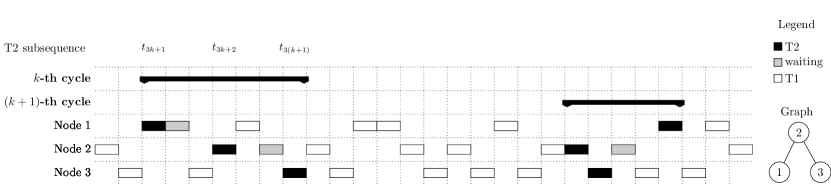
Figure 1: An example of the execution of ASYMM for a network with three nodes.

1. If $\prod_{l=1}^{d_{i}}S_{i}[d_{G},l]\neq 1$, node $i$ performs a gradient descent step on its local augmented Lagrangian (using $1/L_{i}$ as stepsize, where $L_{i}$ is the Lipschitz constant of $\tilde{\mathcal{L}}_{\bm{p}_{\mathcal{N}_{i}}}(x_{\mathcal{N}_{i}},\bm{\theta}_{\mathcal{N}_{i}})$) and checks if the local tolerance $\epsilon_{i}>0$ on the gradient has been reached. If the latter is true, it corresponds to setting $C_{i}\leftarrow 1$ in the distributed logic-AND Algorithm 1. Then, it updates matrix $S_{i}$, and broadcasts the updated $x_{i}$ and the column $S_{i}[:,d_{i}]$ to its neighbors.

2. If $\prod_{l=1}^{d_{i}}S_{i}[d_{G},l]=1$, node $i$ performs an ascent step on the local multiplier vector and updates the local penalty parameters according to equations (6)-(8) and (9)-(11), respectively. Then, it sets $M_{done}=1$ and broadcasts the updated multipliers and penalty parameters $\nu_{ij}$ and $\rho_{ij}$ (associated to constraints $x_{i}=x_{j}$) to its neighbors.

Algorithm 2 ASYMM

Initialize $x_{i}$, $\bm{\theta}_{i}$, $\mathcal{N}_{i}$, $\bm{p}_{i}$, $S_{i}=\bm{0}_{d_{G}\times d_{i}}$, $M_{done}$ = 0.

if $\prod_{b=1}^{d_{i}}S_{i}[d_{G},b]\neq 1$ and not $M_{done}$ then

     $x_{i}\leftarrow x_{i}-\frac{1}{L_{i}}\nabla_{x_{i}}\tilde{\mathcal{L}}_{\bm{p}_{\mathcal{N}_{i}}}(x_{\mathcal{N}_{i}},\bm{\theta}_{\mathcal{N}_{i}})$

     if $\|\nabla_{x_{i}}\tilde{\mathcal{L}}_{\bm{p}_{\mathcal{N}_{i}}}(x_{\mathcal{N}_{i}},\bm{\theta}_{\mathcal{N}_{i}})\|\leq\epsilon_{i}$ then $S_{i}[1,d_{i}]\leftarrow 1$

     

     $S_{i}[l,d_{i}]\leftarrow\prod_{b=1}^{d_{i}}S_{i}[l-1,b]$ for $l=2,...,d_{G}$

     BROADCAST $x_{i}$, $S_{i}[:,d_{i}]$ to all $j\in\mathcal{N}_{i}$

if $\prod_{b=1}^{d_{i}}S_{i}[d_{G},b]=1$ and not $M_{done}$ then

     $\nu_{ij}\leftarrow\nu_{ij}+\rho_{ij}(x_{i}-x_{j})$ for $j\in\mathcal{N}_{i}$

     $\lambda_{i}\leftarrow\lambda_{i}+\varrho_{i}{h}_{i}(x_{i})$

     $\mu_{i}\leftarrow\max\{0,\,\mu_{i}+\zeta_{i}{g}_{i}(x_{i})\}$

     update $\varrho_{i}$, $\zeta_{i}$ and $\rho_{i}$

     $M_{done}$ $\leftarrow$ 1

     BROADCAST $\nu_{ij}$, $\rho_{ij}$ to $j\in\mathcal{N}_{i}$

if $S_{j}[:,d_{j}]$ received from $j\in\mathcal{N}_{i}$ and not already received some new $\nu_{ji}$ then

     $S_{i}[l,j_{i}]\leftarrow S_{j}[l,d_{j}]$ for $l=1,...,d_{G}$

if $\nu_{ji}$ and $\rho_{ji}$ received from $j\in\mathcal{N}_{i}$ set $S_{i}\left[d_{G},:\right]\leftarrow 1$

if $x_{j}^{new}$ received from $j\in\mathcal{N}_{i}$, update $x_{j}\leftarrow x_{j}^{new}$

if $M_{done}$ and $\nu_{ji}$ received from all $j\in\mathcal{N}_{i}$ then

     $M_{done}$ $\leftarrow$ 0, $S_{i}\leftarrow\bm{0}_{d_{G}\times d_{i}}$, update $\epsilon_{i}$

When in IDLE , node $i$ continuously listens for messages from its neighbors, but does not broadcast any information. Received messages may contain either local optimization and logic-AND variables, or multiplier vectors and penalty parameters. If necessary, node $i$ suitably updates local logic-AND variables or the $M_{done}$ flag. Notice that, for node $i$, sending a new multiplier $\nu_{ij}$ or receiving a new $\nu_{ji}$ corresponds to sending or receiving a STOP signal in the asynchronous logic-AND algorithm.

The ASYMM pseudocode is reported in Algorithm 2 and an example of its execution is shown in Figure 1, where tasks T1 and T2 are denoted by white and black blocks, respectively.

Remark 1.

A gossip-based distributed algorithm based on the Method of Multipliers for convex optimization problems has been proposed in [16]. In ASYMM the logic-AND allows the nodes to perform multipliers updates asynchronously, while in [16] a global clock is employed to regulate such an update in a synchronous way. One main advantage of ASYMM is that it guarantees that a prescribed tolerance is reached by each node in the primal descent, which in turn is a crucial feature when solving nonconvex optimization problems.

4 ASYMM Analysis

In order to analyze the ASYMM algorithm, we start by noting that under Assumptions 2 and 3, from a global perspective, the local asynchronous updates can be treated as an algorithmic evolution in which, at each iteration, only one node wakes up in an essentially cyclic fashion.

Given the above, it is possible to associate an iteration of the distributed algorithm to each triggering. Denote by $t\in{\mathbb{N}}$ a discrete, universal time indicating the $t$-th iteration of the algorithm and define as $i_{t}\in\mathcal{V}$ the index of the node triggered at iteration $t$.

In the following, it will be shown that: (i) there is an equivalence relationship between ASYMM and an inexact Method of Multipliers and (ii) under suitable technical conditions, a bound on the gradient of the augmented Lagrangian can be derived from the local tolerances $\epsilon_{i}$.

4.1 Equivalence with an inexact Method of Multipliers

Consider an inexact Method of Multipliers which consists of solving the $k$-th instance of the augmented Lagrangian minimization by means of a block-coordinate gradient descent algorithm (see, e.g., [32] for a survey), which runs for a certain number of iterations $h^{k}$. A pseudo code of this inexact Method of Multipliers (inexact MM) is given in Algorithm 3, where $i_{h}$ is the index of the block chosen at iteration $h$ and the penalty parameters are updated as in (10)-(11).

for $k=0,1,...$ do

     $\hat{\bm{x}}^{0}=\bm{x}^{k}$

     for $h=1,...,h^{k}$ do

         $\hat{\bm{x}}^{h+1}=\hat{\bm{x}}^{h}-\frac{1}{L_{i_{h}}^{k}}U_{i_{h}}\nabla_{x_{i_{h}}}\mathcal{L}_{\bm{p}}(\hat{\bm{x}}^{h},\bm{\theta}^{k})$      

     $\bm{x}^{k+1}=\hat{\bm{x}}^{h^{k}+1}$

     $\nu_{ij}^{k+1}=\nu_{ij}^{k}+\rho_{ij}^{k}(x_{i}^{k+1}-x_{j}^{k+1}),\quad\forall(i,j)\in\mathcal{E}$

     $\lambda_{i}^{k+1}=\lambda_{i}^{k}+\varrho_{i}^{k}{h}_{i}(x_{i}^{k+1}),\forall i\in\mathcal{V}$

     $\mu_{i}^{k+1}=\max\{0,\,\mu_{i}^{k}+\zeta_{i}^{k}{g}_{i}(x_{i}^{k+1})\},\quad\forall i\in\mathcal{V}$

Algorithm 3 Inexact MM

It is worth remarking that the ordered sequence of indexes $h$ and $k$ used in Algorithm 3 does not coincide with the sequence of universal times $t$ of ASYMM. It will be rather shown that a (possibly reordered) subsequence of iterations in the universal time $t$ of ASYMM gives rise to suitable $h$ and $k$ sequences in Algorithm 3.

Let $t_{1},t_{2},...$ be a subsequence of $\{t\}$ such that at each $t_{\ell}$ a multiplier update (task T2) has been performed by node $i_{t_{\ell}}$ and let $t_{1}$ be the time instant of the first multiplier update. Then, the following result holds.

Lemma 3.

Each sequence $(i_{t_{kN+1}},...,i_{t_{(k+1)N}})$, for $k=0,1,...$, is a permutation of $\{1,...,N\}$. Moreover, if $\epsilon_{i}>0$ for all $i\in\mathcal{V}$, multiplier updates occur infinitely many times.

Proof.

Consider the first multiplier update, performed by node $i_{t_{1}}$ at $t_{1}$. Then, until all other nodes have performed their first multiplier update, there will be some node $j$ which has not received back all the new multipliers from its neighbors and has $M_{done}=1$. Hence, it cannot run task T1, and consequently it cannot set and broadcast $S_{j}[1,d_{j}]=1$. So, node $i_{t_{1}}$ has at least one element of the last row of $S_{i_{t_{1}}}$ at $0$, hence it cannot perform another multiplier update (although it could have started over performing task T1). The first part of the proof is completed by induction. In order to prove the second part of the lemma, assume, by contradiction, that the number of multiplier updates is finite and denote by $t_{M}$ the time instant of the last multiplier update. If $\text{mod}(M,N)\neq 0$, from the connectedness of $\mathcal{G}$ at $t_{M}+1$ there exists at least one node $j$ that: i) has not updated its multipliers yet; ii) has a neighbor who has already performed a multiplier update. Hence, node $j$ will perform a multiplier update next time it wakes up (which occurs in finite time by Assumption 2), thus contradicting the assumption that $t_{M}$ was the time instant of the last multiplier update. If $\text{mod}(M,N)=0$ (i.e., $(i_{t_{M-N+1}},\dots,i_{t_{M-1}},i_{t_{M}})$ is a permutation of $\{1,\ldots,N\}$), all the nodes that wake up after $t_{M}$ will run task T1. From a global perspective, this can be seen as a block coordinate descent algorithm on the augmented Lagrangian with a given multiplier vector. Since this algorithm converges to a stationary point [33], every node $i\in\mathcal{V}$ will reach its local tolerance $\epsilon_{i}>0$ in finite time and then set $S_{i}[1,d_{i}]=1$. From Proposition 1, after a finite number of iterations some node $j$ will satisfy $\prod_{b=1}^{d_{j}}S_{j}[d_{G},b]=1$ and hence it will run a new multiplier update, which contradicts the assumption that $t_{M}$ was the time instant of the last multiplier update. ∎

In the sequel the subset of universal times $t$, $\{{t_{kN+1}},...,{t_{(k+1)N}}\}$, during which $N$ tasks T2 are performed, will be referred to as the $k$-th cycle of ASYMM.

The example in Figure 1 shows the $k$-th and $(k{+}1)$-th cycles of an ASYMM run. According to Lemma 3, during a single cycle each node performs task T2 once. It is worth remarking that in the $k$-th cycle node $1$ starts over the $(k{+}1)$-th primal minimization before node $3$ has completed its $k$-th multiplier update. This happens because node $1$ has already received the updated multipliers and penalty parameters from node $2$, which is the only neighbor of node $1$. The same thing happens to node $3$ in the $(k{+}1)$-th cycle. This is a key feature of the asynchronous distributed scheme underlying ASYMM. It can also be observed that when node $3$ wakes up for the first time, after node $1$ has done the $k$-th dual update, it performs again task T1. In fact, node $3$ has not received a STOP signal yet, because it is not connected directly to node $1$.

Define $\bm{\theta}_{i}=[\lambda_{i},\mu_{i},\nu_{i}]$ and let $\tilde{x}_{i}^{t}$ and $\tilde{\bm{\theta}}_{i}^{t}$ be the value of the state vector and of the multiplier vector of node $i$, at iteration $t$, computed according to ASYMM. Then, the following Corollary holds, whose proof follows immediately from Lemma 3.

Corollary 4.

Let $\tau\in\{t_{kN+1},...,t_{(k+1)N}\}$, for some $k=0,1,...$. Then one has $\tilde{\bm{\theta}}_{i_{\tau}}^{t}=\tilde{\bm{\theta}}_{i_{\tau}}^{\tau}$ for all $t=\tau,\tau{+}1,\dots,t_{(k+1)N}$. $\square$

Corollary 4 states that once a multiplier vector is updated in a cycle, then, its value remains unchanged for the whole cycle.

Let ${\tau_{i}^{k}}$ be the time instant in which node $i$ performs task T2 in the $k$-th cycle, i.e., ${\tau_{i}^{k}}\in\{t_{kN+1},...,t_{(k+1)N}\}$ such that node $i$ is awake at time ${\tau_{i}^{k}}$. By using this Corollary 4, one can define

$$x_{i}^{k+1}=\tilde{x}_{i}^{\tau_{i}^{k}},\quad\bm{\theta}_{i}^{k+1}=\tilde{\bm{\theta}}_{i}^{\tau_{i}^{k}},$$

$k=0,1,...$ and by using Lemma 3 and reordering the indexes $i_{\tau}$,

$$\bm{x}^{k+1} =\left[\left(x_{1}^{k+1}\right)^{\top},...,\left(x_{N}^{k+1}\right)^{\top}\right]^{\top},$$

$$\bm{\theta}^{k+1} =\left[\left(\bm{\theta}_{1}^{k+1}\right)^{\top},...,\left(\bm{\theta}_{N}^{k+1}\right)^{\top}\right]^{\top}.$$

The next two lemmas show that a local primal (resp. multiplier) update is performed according to a common multiplier (resp. primal) variable.

Lemma 5.

For all $\tau\in\{t_{kN+1},...,t_{(k+1)N}\}$, $k=0,\!1,...$, every multiplier $\bm{\theta}_{i_{\tau}}^{k+1}$ is computed using the state vector $\bm{x}^{k+1}$.

Proof.

Consider $\tau\in\{t_{kN+1},...,t_{(k+1)N}\}$ for a given $k$. Node $i_{\tau}$ computes

$$x_{i_{\tau}}^{k+1} =\tilde{x}_{i_{\tau}}^{\tau},$$

$$\nu_{i_{\tau}j}^{k+1} =\nu_{i_{\tau}j}^{k}+\rho_{i_{\tau}j}^{k}(x_{i_{\tau}}^{k+1}-\tilde{x}_{j}^{\tau}), \forall j\in\mathcal{N}_{i_{\tau}},$$

$$\lambda_{i_{\tau}}^{k+1} =\lambda_{i_{\tau}}^{k}+\varrho_{i_{\tau}}^{k}{h}_{i_{\tau}}(x_{i_{\tau}}^{k+1}),$$

$$\mu_{i_{\tau}}^{k+1} =\max\{0,\,\mu_{i_{\tau}}^{k}+\zeta_{i_{\tau}}^{k}{g}_{i_{\tau}}(x_{i_{\tau}}^{k+1})\}.$$

First, notice that the update of node $i_{\tau}$ depends only on $x_{j}$ or $\bm{\theta}_{j}$ with $j\in\mathcal{N}_{i_{\tau}}$. Then, let us show that $\tilde{x}_{j}^{\tau}=x_{j}^{k+1}$ for all $j\in\mathcal{N}_{i_{\tau}}$. If a node $j\in\mathcal{N}_{i_{\tau}}$ has already performed its multiplier update in the $k$-th cycle, then, even if it woke up again before time $\tau$ it did not update $x_{j}$ (did not start a new primal update) because it has not received all the updated multipliers from its neighbors (node $i_{\tau}$ has not performed the multiplier update yet and thus has not sent $\nu_{i_{\tau}j}^{k+1}$ to node $j$). Therefore, $\tilde{x}_{j}^{\tau}=x_{j}^{k+1}$. If, vice-versa, node $j\in\mathcal{N}_{i_{\tau}}$ has not performed its multiplier update in the $k$-th cycle, then $\tilde{x}_{j}^{\tau}$ will become $x_{j}^{k+1}$ next time node $j$ wakes up (because node $i_{\tau}$ has sent it the updated multiplier while it was in idle, so that $j$ has set $S_{j}[d_{G},:]=1$). ∎

Lemma 6.

For all $t=\tau_{i}^{k},\tau_{i}^{k}+1,\dots,\tau_{i}^{k+1}$, every descent step on the augmented Lagrangian with respect to the block-coordinate $x_{i}$ is performed using the multiplier vector $\bm{\theta}^{k+1}$.

Proof.

Node $i$ can start over a block coordinate descent iteration after $\tau_{i}^{k}$ only when it has received all the new multipliers $\nu_{ji}^{k+1}$ (and the corresponding penalty parameters) from its neighbors. Thanks to (15), it is sufficient to show that each local descent on the $i$-th local augmented Lagrangian is performed using the multiplier vector $\bm{\theta}_{\mathcal{N}_{i}}^{k+1}$. This follows from Lemma 3 and Corollary 4 by using arguments similar to those in the proof of Lemma (5). ∎

Next lemma states that every node performs at least one primal update between the beginning of two consecutive cycles.

Lemma 7.

Between $t_{kN+1}$ and $t_{(k+1)N+1}$ every node performs task $T1$ at least once.

Proof.

Since at iteration $t_{(k+1)N}$ all the nodes have performed the $k$-th multiplier update, each of them has set $S_{i}[1,d_{i}]=0$ at some time between $t_{kN+1}$ and $t_{(k+1)N}$. At time $t_{(k+1)N+1}$ the first node performs the $(k+1)$-th multiplier update. This can occur only if each node $i$ has set $S_{i}[1,d_{i}]=1$ at some time between $t_{kN+1}$ and $t_{(k+1)N+1}$, which implies that each node performs task T1 at least once over the same time interval. ∎

The equivalence of ASYMM and Algorithm 3 is stated by the next theorem.

Theorem 8.

Let Assumptions 2 and 3 hold. Then, ASYMM is equivalent to an instance of Algorithm 3 in which the selection of nodes $i_{h}$ satisfies an essentially cyclic rule. Moreover, if in Algorithm 2, $\epsilon_{i}>0$, $\forall i\in\mathcal{V}$, the total number of primal descent steps $h^{k}$ is finite.

Proof.

Define $H_{i}^{k}{=}\{t\mid\tau_{i}^{k-1}{<}t{<}\tau_{i}^{k},\,i\text{ runs task T1 at }t\}$ for $k=0,1,...$, where $\tau_{i}^{-1}$ is the first time instant in which node $i$ is awake (doing task T1). Then, define ${H}^{k}=\bigcup_{i\in\mathcal{V}}H_{i}^{k}$, $h^{k}=|{H}^{k}|$ and let

$$\upsilon_{1}<\upsilon_{2}<...<\upsilon_{h^{k}}\$$

be the ordered sequence of elements (time instants) in ${H}^{k}$.

By setting $i_{h}=i_{v_{h}}$, for $h=1,\dots,h^{k}$, in Algorithm 3 and using Lemma 5 and Lemma 6, one has that ASYMM turns out to be equivalent to an instance of Algorithm 3. Moreover, from Lemma 7 every node runs task T1 at least once in $\{v_{1},\dots,v_{h^{k}}\}$. Hence, Algorithm 3 is run with an essentially cyclic update rule over a time window of length $h_{k}$, which is finite due to Lemma 3. ∎

Remark 2.

The duration of each ASYMM cycle can be bounded both from below and from above as follows. From the definition of $h^{k}$ it can be easily verified that $h^{k}\geq N$. Moreover, from Lemma 7 one has that $h^{k}\leq t_{(k+1)N+1}-t_{kN+1}-N$. Hence, $t_{(k+1)N+1}-t_{kN+1}\geq 2N$. On the other side, from Proposition 1 it follows that $t_{(k+1)N}-t_{kN+1}\leq d_{G}\bar{T}$ for all $k$.

4.2 A bound on the Lagrangian gradient

In virtue of the equivalence result in Theorem 8, ASYMM inherits the convergence properties of Algorithm 3 applied to Problem 2. In particular, in order to guarantee the convergence of the inexact MM to a local minimum, it is necessary that the Lagrangian minimization is asymptotically exact (see, e.g., [26, Section 2.5]). To this aim, in this section an upper bound $\varepsilon$ on the norm of the gradient of the augmented Lagrangian (4) is derived as a function of the local tolerances $\epsilon_{i}$ employed in task T1 of ASYMM. The result requires (at a given iteration $k$) a technical assumption of local (strong) convexity of the augmented Lagrangian.

Let us introduce the following preliminary result.

Lemma 9.

Let $\Phi(y_{1},\ldots,y_{N})$ be a $\sigma$-strongly convex function with block component-wise Lipschitz continuous gradients (with $L_{i}$ being the Lipschitz constant with respect to block $y_{i}$) in a subset $Y\subseteq\mathbb{R}^{n}$. Let $\{\bm{y}^{h}\}$ be a sequence generated according to $\bm{y}^{h+1}=\bm{y}^{h}-\frac{1}{L_{i_{h}}}U_{i_{h}}\nabla_{y_{i_{h}}}\Phi(\bm{y}^{h})$, where $\bm{y}^{0}\in Y$ and indexes $i_{h}\in\{1,\ldots,N\}$ are drawn in an essentially cyclic way. If, for some $\bar{h}_{i}>0$, $\|\nabla_{y_{i}}\Phi(\bm{y}^{\bar{h}_{i}})\|\leq\epsilon_{i},\;\forall i\in\{1,\ldots,N\}$, then

$$\|\nabla_{\bm{y}}\Phi(\bm{y}^{h})\|\leq\sqrt{\sum_{i=1}^{N}\left(\frac{L_{i}\epsilon_{i}}{\sigma}\right)^{2}}$$

for all $h\geq\bar{h}=\max_{i\in\{1,\ldots,N\}}\bar{h}_{i}$.

Proof.

See the Appendix. ∎

The next result provides a bound on the norm of the gradient of the augmented Lagrangian $\mathcal{L}(\bm{x},\bm{\theta})$ used in ASYMM.

Proposition 10.

Let Assumption 1 hold and assume that $\bm{x}^{k}$ generated by ASYMM belongs to a neighborhood of a local minimum of $\mathcal{L}_{\bm{p}^{k}}(\bm{x},\bm{\theta}^{k})$ where $\mathcal{L}_{\bm{p}^{k}}(\bm{x},\bm{\theta}^{k})$ is $\sigma^{k}$-strongly convex. Denote by $\epsilon_{i}^{k}$ the local tolerance set by node $i$ for the primal descent during cycle $k$ and by $L_{i}^{k}$ the Lipschitz constant of $\nabla_{x_{i}}\tilde{\mathcal{L}}_{\bm{p}_{\mathcal{N}_{i}}^{k}}(x_{\mathcal{N}_{i}},\bm{\theta}_{\mathcal{N}_{i}}^{k})$. Then, it holds

$$\|\nabla_{\bm{x}}\mathcal{L}_{\bm{p}^{k}}(\bm{x}^{k+1},\bm{\theta}^{k})\|\leq\varepsilon^{k}=\sqrt{\sum_{i=1}^{N}\left(\frac{L_{i}^{k}\epsilon_{i}^{k}}{\sigma^{k}}\right)^{2}}.$$

Proof.

From Proposition 2, $\mathcal{L}_{\bm{p}^{k}}(\bm{x},\bm{\theta}^{k})$ has block component-wise Lipschitz continuous gradient with constants $L_{i}^{k}$. Moreover, during the $k$-th cycle of ASYMM, there occurred that $\|\nabla_{x_{i}}\tilde{\mathcal{L}}_{\bm{p}_{\mathcal{N}_{i}}^{k}}(x_{\mathcal{N}_{i}},\bm{\theta}_{\mathcal{N}_{i}}^{k})\|\leq\epsilon_{i}^{k}$ and hence, by (15), also $\|\nabla_{x_{i}}\mathcal{L}_{\bm{p}^{k}}(\bm{x},\bm{\theta}^{k})\|\leq\epsilon_{i}^{k}$. Then, being $\bm{x}^{k+1}$ generated through a block coordinate descent (according to Theorem 8), the proof follows from Lemma 9. ∎

Proposition 10 relates the local tolerances adopted by the nodes in the primal descent to a global bound on the norm of the gradient of the augmented Lagrangian. The result requires to assume that the vector $\bm{x}^{k}$ generated during the $k$-th cycle of ASYMM lies in a neighborhood of a local minimum of the current augmented Lagrangian, in which the augmented Lagrangian itself is strongly convex. This assumption is indeed strong, but it is somehow standard in the nonconvex optimization literature (see, e.g., [26, Section 2.2.4]). In practice it turns out to be typically satisfied after a sufficient number of iterations of multiplier/penalty parameter updates. In fact, as $\bm{p}^{k}$ grows according to the update rules (9)-(11), the augmented Lagrangian tends to become locally strongly convex. Moreover, from a practical point of view, it has been observed that choosing the obtained $\bm{x}^{k}$ as the initial condition for the $(k{+}1)$-th minimization usually generates sequences $\{\bm{x}^{k}\}$ that remain within a neighborhood of the same local minimum of Problem (2), thus meaning that there exists a cycle $\bar{k}$ after which the assumption in Proposition 10 will hold indefinitely. Hence, if the assumptions of Proposition 10 hold from a certain cycle $\bar{k}$ and the local tolerances $\epsilon_{i}^{k}$ vanish as $k\to\infty$, the minimization of the augmented Lagrangian turns out to be asymptotically exact. Therefore, convergence results such those in [26, Section 2.5] can be recovered, when applying ASYMM to Problem (2). The interested reader is referred to [26, Chapter 2] for a thorough discussion on the convergence properties of the Method of Multipliers.

5 Dealing with big-data optimization

The ASYMM algorithm can be easily amended to deal with so called distributed big-data optimization, [34], i.e., the distributed solution of problems in which $x\in\mathbb{R}^{n}$ with $n$ very large. In this set up arising, e.g., in estimation and learning problems, two main problems may arise. On one hand, the primal and multiplier update steps may not be executable in a single step by some node because the computation of the whole gradient in the primal step may be cumbersome. Moreover, communication bottlenecks may arise, in fact it may happen for some node $i$, that the local optimization variable $x_{i}$ does not fit the communication channels between node $i$ and its neighbors.

Assume each agent $i$ to partition its local decision variable $x_{i}$ in $N_{i}$ blocks, i.e., $x_{i}=\left[x_{i,1}\dots x_{i,N_{i}}\right]^{\top}$, where $x_{i,m}=U_{i,m}^{\top}x_{i}$ and $x_{i}=\sum_{m=1}^{N_{i}}U_{i,m}x_{i,m}$.

Whenever node $i$ wakes up to perform task T1, it computes the primal descent step on one of the $N_{i}$ blocks (say $m$) instead of performing it on the whole $x_{i}$, i.e. it computes

$$x_{i,m}=x_{i,m}-\frac{1}{L_{i,m}}\nabla_{x_{i,m}}\tilde{\mathcal{L}}_{\bm{p}_{\mathcal{N}_{i}}}(x_{\mathcal{N}_{i}},\bm{\theta}_{\mathcal{N}_{i}})$$

where $m$ is picked in an essentially cyclic way. Similarly the update of the local multiplier vectors can be carried out on one block at a time, e.g.,

$$\nu_{ij,m}\leftarrow\nu_{ij,m}+\rho_{ij}(x_{i,m}-x_{j,m}).$$

By following the same reasoning adopted in Sections $3$ and $4$, it can be shown that the primal descent steps are equivalent to a block coordinate descent algorithm on the augmented Lagrangian and converge to a stationary point.

The only additional assumption needed for the convergence result is that functions $f_{i}$, ${h}_{i}$, ${g}_{i}$ have block component-wise Lipschitz continuous gradients. If for some node $i$, $x_{i}$ does not fit the communication channels (the same holds true for $\nu_{ij}$), ASYMM is easily extended by allowing node $i$ to transmit $x_{i,m}$ and $U_{i,m}$ at the end of each task T1 and to split the transmission on $\nu_{ij}$ in multiple steps.

6 Numerical Results

Two examples are presented to assess the performance of ASYMM. The first one involves nonconvex local constraints, while the second requires the minimization of a nonconvex objective function.

6.1 Distributed source localization

Consider a network of $N$ sensors, deployed over a certain region, communicating according to a connected graph $\mathcal{G}=(\mathcal{V},\mathcal{E})$, which have to solve the optimization problem

$$\mathop{\rm minimize}_{x} \sum_{i=1}^{N}f_{i}(x)$$

subject to $$\|x-c_{i}\|-R_{i}\leq 0, i=1,...,N$$

$$r_{i}-\|x-c_{i}\|\leq 0, i=1,...,N,$$

which can be rewritten in the form of problem (2).

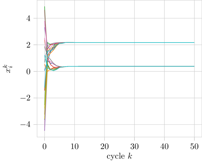
(a) Evolution of the local decision variables $x_{i}^{k}$.

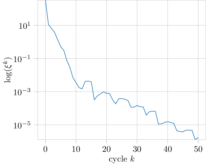
(b) Logarithm of the measure of infeasibility $\xi^{k}$.

Figure 2: Distributed source localization

Such a problem naturally arises, for example, in the context of source localization, in which each agent knows its own absolute location $c_{i}$ and takes a noisy measurement $y_{i}$ of its own distance from an an emitting source located at an unknown location $x^{\star}$ (for example through a laser) as $y_{i}=\|x^{\star}-c_{i}\|+w_{i}$. If we make the assumption of unknown but bounded (UBB) noise, i.e. for all $i=1,...,N$, the noise signal $w_{i}$ satisfies $|w_{i}|\leq\kappa_{i}$ for some $\kappa_{i}\geq 0$, then each node is able to define its own feasible set $X_{i}$ in which the unknown source location must lie as $X_{i}=\{x\mid r_{i}\leq\|x-c_{i}\|\leq R_{i}\}$, where $r_{i}=y_{i}-\kappa_{i}$ and $R_{i}=y_{i}+\kappa_{i}$. Notice that each set $X_{i}$ is a circular crown and hence it is a non convex set.

Suppose $f_{i}(x_{i})=x_{i}^{\top}x_{i}$ for all $i\in\mathcal{V}$. We report a simulation with $N=10$ nodes and $n=2$, in which $x^{\star}\in U[-2.5,2.5]^{n}$, $c_{i}\in U[-2.5,2.5]^{n}$ and $\kappa_{i}\in U[0,0.3]$ for all $i\in\mathcal{V}$, where $U[a,b]$ denotes the uniform distribution between $a$ and $b$. The graph is modeled through a connected Watts-Strogatz model in which nodes has mean degree $K=2$. Let us define the measure of infeasibility at iteration $k$ as

$$\xi^{k}= \sum_{i=1}^{N}\bigg{(}\max(0,\|x_{i}^{k}-c_{i}\|-R_{i})+$$

$$+\max(0,r_{i}-\|x_{i}^{k}-c_{i}\|)+\sum_{j\in\mathcal{N}_{i}}\|x_{i}^{k}-x_{j}^{k}\|\bigg{)}$$

We run ASYMM for $25000$ iterations with $\beta=4$ and $\gamma=0.25$. Figure 2(a) shows the evolution of $x_{i}^{k}$ for each $i\in\mathcal{V}$. Finally, in Figure 2(b) the values of $\xi^{k}$ are reported. As it can be seen, the nodes performed $50$ multiplier updates each, along the $25000$ iterations (corresponding to 2500 awakenings per node on average).

6.2 Distributed nonlinear classification

In this example we consider a nonlinear classification problem in which the data to be classified are represented as points $z\in\mathbb{R}^{2}$ which belong to two different classes. So, each point is associated a label $y\in\{-1,1\}$, which represents the class the point belongs to.

The considered classifier can be represented as a Neural Network (NN) consisting of one input layer with two units, two hidden layers with four and two units respectively, and an output layer with one unit (respectively green, blue and red in Figure 3). Moreover, a bias unit is present in both the input and the hidden layers (in yellow in Figure 3). Define $w_{1}\in\mathbb{R}^{2\times 4}$, $b_{1}\in\mathbb{R}^{4}$, $w_{2}\in\mathbb{R}^{4\times 2}$, $b_{2}\in\mathbb{R}^{2}$, $w_{3}\in\mathbb{R}^{2\times 1}$ and $b_{3}\in\mathbb{R}$. Moreover, define $x\in\mathbb{R}^{25}$ as the stack of all the previously defined variables.

Define the output of the first hidden layer as

$$l_{1}(z,w_{1},b_{1})=\tanh(w_{1}^{\top}z+b_{1}).$$ (18)

where the operator $\tanh$ is to be intended component-wise. Similarly, the output of the second hidden layer is

$$l_{2}(z,w_{1},b_{1},w_{2},b_{2})=\tanh(w_{2}^{\top}l_{1}(z,w_{1},b_{1})+b_{2})$$ (19)

and the output of the whole NN is

$$f(z,x)=\tanh(w_{3}^{\top}l_{2}(z,w_{1},b_{1},w_{2},b_{2})+b_{3})$$ (20)

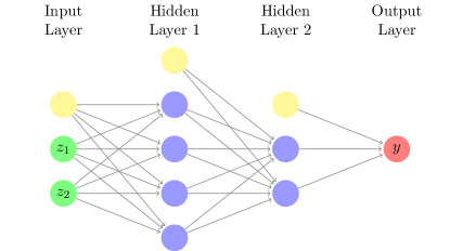
Figure 3: Graphical representation of the Neural Network used as classifier. In green the input units, in blue the hidden units, in red the output unit and in yellow the bias units.

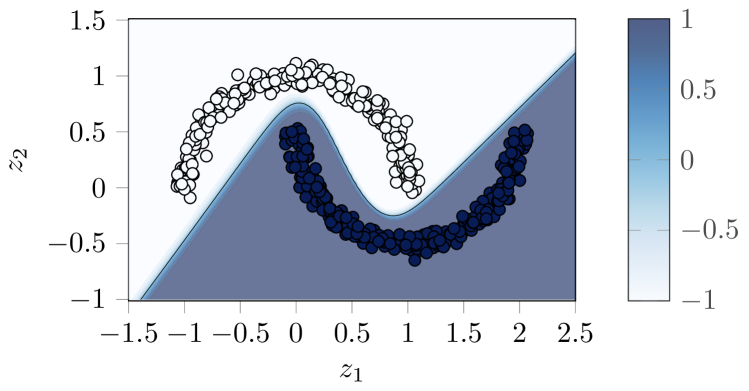
(a) Two moons dataset.

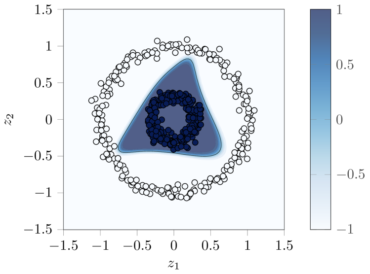
(b) Nested circles dataset.

Figure 4: Distributed nonlinear classification. Blue dots represent points with label $-1$ and white dots points with label $1$. Colored regions represent the output of the classifier (20) resulting from the solution of (22) provided by ASYMM. The color of the regions is associated to a number as in the color bar.

Given a set of labeled data points $(Z,Y)$, the classification problem can be written as

$$\mathop{\rm minimize}_{x}\sum_{z,y\in(Z,Y)}\left(f(z,x)-y\right)^{2}.$$ (21)

Suppose now that the dataset is distributed among $N$ nodes, which communicate according to a connected graph $\mathcal{G}=(\mathcal{V},\mathcal{E})$. Each node $i$ owns a portion of the dataset $(Z_{i},Y_{i})$, which must remain private and cannot be shared with the other nodes. In this framework, problem (21) can be rewritten in the equivalent form

$$\mathop{\rm minimize}_{x_{1},\dots,x_{N}} \sum_{i=1}^{N}\sum_{z,y\in(Z_{i},Y_{i})}\left(f(z,x_{i})-y\right)^{2}$$ (22)

subject to $$x_{i}=x_{j},\qquad\forall(i,j)\in\mathcal{E}$$

In our simulations two datasets are considered, which are benchmarks used in the context of machine learning. The first one consists of points belonging to two moon-shaped subsets (see Figure 4(a)), in which points of one subset have label $y=1$, points of the other have label $y=-1$. In the second one, data points are distributed along two nested circles. Points on the inner circle have label $y=1$, while the others have label $y=-1$ (see Figure 4(b)).

The ASYMM algorithm has been run on $N=10$ nodes, each one processing a local dataset $(Z_{i},Y_{i})$ consisting of 100 points. The obtained classifiers are represented in Figures 4(a) and 4(b). The colored regions represent the value of (20) computed in those points at the (local) minimum $x^{\star}$ obtained by ASYMM.

It is worth stressing that the example presents a low-size classification problem, with the purpose of illustrating the proposed technique. When massive data in higher dimensional spaces are available, it is necessary to consider a more complex neural network (i.e., with a much higher number of neurons) so that the dimension of the decision variable can be fairly high. In such a case, the big-data approach proposed in Section 5 can be adopted.

7 Conclusions

In this paper, an asynchronous distributed algorithm for nonconvex optimization problems over networks has been proposed. By suitably defining local augmented Lagrangian functions, the optimization process has been distributed among the agents of the network. A fully asynchronous implementation has been devised, taking advantage of a distributed logic-AND algorithm that allows the agents to regulate the sequence of primal and dual update steps. The proposed ASYMM algorithm is shown to be equivalent to an inexact version of the centralized method of multipliers, thus inheriting its main properties. An extension to big-data problems, featuring high-dimensional decision variables, has been also presented.

Ongoing research concerns the specialization of the proposed method to different application domains, including distributed set membership estimation and machine learning with constraints.

Appendix

Proof of Lemma 9

Consider a function $\Phi(y)$, $\sigma$-strongly convex in a subset $Y\subseteq\mathbb{R}^{n}$, with $L$-Lipschitz continuous gradient. Define $y^{\star}=\arg\min_{y\in Y}\Phi(y)$. From the definition, if $\Phi(y)$ is $\sigma$-strongly convex, then, using the Cauchy Schwartz inequality one obtains

$$\|\nabla\Phi(y)-\nabla\Phi(z)\|\geq\sigma\|y-z\|.$$

Then, it can be easily proved that

$$\sigma\|y-y^{\star}\|\leq\|\nabla\Phi(y)\|\leq L\|y-y^{\star}\|,\;\forall y\in Y$$ (23)

In order to prove Lemma 9 the following technical results are needed.

Lemma 11.

Performing a gradient descent algorithm on $\Phi(y)$, starting from $y^{0}$ and using a step-size equal to $\frac{1}{L}$, i.e.

$$y^{h+1}=y^{h}-\frac{1}{L}\nabla_{y}\Phi(y^{h})$$ (24)

produces a sequence $\{y^{h}\}$ such that,

$$\|y^{h+1}-y^{\star}\|\leq\|y^{h}-y^{\star}\|$$ (25)

Proof.

See, e.g., [35, Theorem 2.1.14]. ∎

Lemma 12.

Consider a sequence $\{y^{h}\}$ generated as $y^{h+1}=y^{h}-\frac{1}{L}\nabla\Phi(y^{h})$ with $y^{0}\in Y$. Then:

1. for all $h\geq\bar{h}$ it holds that

   $$\|\nabla\Phi(y^{h})\|\leq L\|y^{\bar{h}}-y^{\star}\|$$ (26)

2. if for some $\bar{h}$ it holds that $\|\nabla\Phi(y^{\bar{h}})\|=\varepsilon$, then

   $$\|\nabla\Phi(y^{h})\|\leq\frac{L\varepsilon}{\sigma}$$ (27)

   for all $h\geq\bar{h}$.

Proof.

Using the right side of (23) and Lemma 11 one has that

$$\|\nabla\Phi(y^{\bar{h}+1})\|\leq L\|y^{\bar{h}+1}-y^{\star}\|\leq L\|y^{\bar{h}}-y^{\star}\|$$

By induction, (26) follows directly and this concludes the proof for point 1. For point (ii), since $\|\nabla\Phi(y^{\bar{h}})\|=\varepsilon$, from the left side of (23), one has that

$$\sigma\|y^{\bar{h}}-y^{\star}\|\leq\varepsilon$$

which can be rewritten as

$$\|y^{\bar{h}}-y^{\star}\|\leq\frac{\varepsilon}{\sigma}$$ (28)

Then, substituting (28) in the right side of (23), we obtain (27) which, from point 1 concludes the proof. ∎

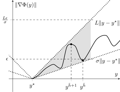
Figure 5: Representation of the results of Lemma 12.

A graphical representation of the previous Lemma is given in Figure 5. The gradient of $\Phi(y)$ is bounded by the dotted lines, as from (23). Moreover, from (25), given $\|\nabla_{y}\Phi(y^{\bar{h}})\|$, it holds that $\|\nabla_{y}\Phi(y^{\bar{h+1}})\|$ stays in the shaded region.

Finally, Lemma 9 is proved by noting that, from Lemma 12

$$\|\nabla_{y_{i}}\Phi(\bm{y}^{{h}})\|\leq\frac{L_{i}\epsilon_{i}}{\sigma}$$

for all $h\geq\bar{h}_{i}$, and

$$\|\nabla_{\bm{y}}\Phi(\bm{y}^{h})\|=\sqrt{\sum_{i=1}^{N}\|\nabla_{y_{i}}\Phi(\bm{y}^{{h}})\|^{2}}.$$

References

- [1] S. Lee and A. Nedic, “Distributed random projection algorithm for convex optimization,” IEEE Journal of Selected Topics in Signal Processing, vol. 7, no. 2, pp. 221–229, 2013.
- [2] K. Margellos, A. Falsone, S. Garatti, and M. Prandini, “Distributed constrained optimization and consensus in uncertain networks via proximal minimization,” IEEE Transactions on Automatic Control, vol. PP, no. 99, pp. 1–1, 2017.
- [3] A. Nedic and A. Ozdaglar, “Distributed subgradient methods for multi-agent optimization,” IEEE Transactions on Automatic Control, vol. 54, no. 1, pp. 48–61, 2009.
- [4] P. Lin, W. Ren, and Y. Song, “Distributed multi-agent optimization subject to nonidentical constraints and communication delays,” Automatica, vol. 65, pp. 120 – 131, 2016.
- [5] I. Necoara, “Random coordinate descent algorithms for multi-agent convex optimization over networks,” IEEE Transactions on Automatic Control, vol. 58, no. 8, pp. 2001–2012, 2013.
- [6] T.-H. Chang, A. Nedić, and A. Scaglione, “Distributed constrained optimization by consensus-based primal-dual perturbation method,” IEEE Transactions on Automatic Control, vol. 59, no. 6, pp. 1524–1538, 2014.
- [7] D. Yuan, D. W. Ho, and S. Xu, “Regularized primal-dual subgradient method for distributed constrained optimization.” IEEE Trans. Cybernetics, vol. 46, no. 9, pp. 2109–2118, 2016.
- [8] C.-X. Shi and G.-H. Yang, “Augmented lagrange algorithms for distributed optimization over multi-agent networks via edge-based method,” Automatica, vol. 94, pp. 55 – 62, 2018.
- [9] A. Falsone, K. Margellos, S. Garatti, and M. Prandini, “Dual decomposition for multi-agent distributed optimization with coupling constraints,” Automatica, vol. 84, pp. 149 – 158, 2017.
- [10] F. Iutzeler, P. Bianchi, P. Ciblat, and W. Hachem, “Explicit convergence rate of a distributed alternating direction method of multipliers,” IEEE Transactions on Automatic Control, vol. 61, no. 4, pp. 892–904, 2016.
- [11] P. Bianchi, W. Hachem, and I. Franck, “A stochastic coordinate descent primal-dual algorithm and applications,” in Machine Learning for Signal Processing (MLSP), 2014 IEEE International Workshop on. IEEE, 2014, pp. 1–6.
- [12] P. Bianchi, W. Hachem, and F. Iutzeler, “A coordinate descent primal-dual algorithm and application to distributed asynchronous optimization,” IEEE Transactions on Automatic Control, vol. 61, no. 10, pp. 2947–2957, 2016.
- [13] D. P. Bertsekas and J. N. Tsitsiklis, Parallel and distributed computation: numerical methods. Prentice hall Englewood Cliffs, NJ, 1989, vol. 23.
- [14] S. Boyd, A. Ghosh, B. Prabhakar, and D. Shah, “Randomized gossip algorithms,” IEEE transactions on information theory, vol. 52, no. 6, pp. 2508–2530, 2006.
- [15] A. Nedic, “Asynchronous broadcast-based convex optimization over a network,” IEEE Transactions on Automatic Control, vol. 56, no. 6, pp. 1337–1351, 2011.
- [16] D. Jakovetic, J. Xavier, and J. M. Moura, “Cooperative convex optimization in networked systems: Augmented lagrangian algorithms with directed gossip communication,” IEEE Transactions on Signal Processing, vol. 59, no. 8, pp. 3889–3902, 2011.
- [17] E. Wei and A. Ozdaglar, “On the convergence of asynchronous distributed alternating direction method of multipliers,” in Global conference on signal and information processing (GlobalSIP), 2013 IEEE. IEEE, 2013, pp. 551–554.
- [18] I. Notarnicola and G. Notarstefano, “Asynchronous distributed optimization via randomized dual proximal gradient,” IEEE Transactions on Automatic Control, vol. 62, no. 5, pp. 2095–2106, 2017.
- [19] P. Bianchi and J. Jakubowicz, “Convergence of a multi-agent projected stochastic gradient algorithm for non-convex optimization,” IEEE Transactions on Automatic Control, vol. 58, no. 2, pp. 391–405, 2013.
- [20] H.-T. Wai, A. Scaglione, J. Lafond, and E. Moulines, “A projection-free decentralized algorithm for non-convex optimization,” in Signal and Information Processing (GlobalSIP), 2016 IEEE Global Conference on. IEEE, 2016, pp. 475–479.
- [21] P. Di Lorenzo and G. Scutari, “Next: In-network nonconvex optimization,” IEEE Transactions on Signal and Information Processing over Networks, vol. 2, no. 2, pp. 120–136, 2016.
- [22] Y. Sun, G. Scutari, and D. Palomar, “Distributed nonconvex multiagent optimization over time-varying networks,” in Signals, Systems and Computers, 2016 50th Asilomar Conference on. IEEE, 2016, pp. 788–794.
- [23] T. Tatarenko and B. Touri, “Non-convex distributed optimization,” IEEE Transactions on Automatic Control, vol. 62, no. 8, pp. 3744–3757, 2017.
- [24] I. Notarnicola and G. Notarstefano, “A randomized primal distributed algorithm for partitioned and big-data non-convex optimization,” in Decision and Control (CDC), 2016 IEEE 55th Conference on. IEEE, 2016, pp. 153–158.
- [25] D. P. Bertsekas, “Multiplier methods: A survey,” Automatica, vol. 12, no. 2, pp. 133 – 145, 1976.
- [26] ——, Constrained optimization and Lagrange multiplier methods. Academic press, 2014.
- [27] R. T. Rockafellar, “Augmented lagrange multiplier functions and duality in nonconvex programming,” SIAM Journal on Control, vol. 12, no. 2, pp. 268–285, 1974.
- [28] I. Matei, J. S. Baras, M. Nabi, and T. Kurtoglu, “An extension of the method of multipliers for distributed nonlinear programming,” in Decision and Control (CDC), 2014 IEEE 53rd Annual Conference on. IEEE, 2014, pp. 6951–6956.
- [29] I. Matei and J. S. Baras, “Distributed nonlinear programming methods for optimization problems with inequality constraints,” in Decision and Control (CDC), 2015 IEEE 54th Annual Conference on. IEEE, 2015, pp. 2649–2654.
- [30] T. Ayken and J.-I. Imura, “Diffusion based stopping criterion for event-triggered distributed optimization,” SICE Journal of Control, Measurement, and System Integration, vol. 8, no. 6, pp. 371–379, 2015.
- [31] G. Oliva, R. Setola, and C. N. Hadjicostis, “Distributed finite-time calculation of node eccentricities, graph radius and graph diameter,” Systems & Control Letters, vol. 92, pp. 20–27, 2016.
- [32] S. J. Wright, “Coordinate descent algorithms,” Mathematical Programming, vol. 151, no. 1, pp. 3–34, 2015.
- [33] Y. Xu and W. Yin, “A globally convergent algorithm for nonconvex optimization based on block coordinate update,” Journal of Scientific Computing, pp. 1–35, 2017.
- [34] I. Notarnicola, Y. Sun, G. Scutari, and G. Notarstefano, “Distributed big-data optimization via block-iterative convexification and averaging,” in 2017 IEEE 56th Annual Conference on Decision and Control (CDC), 2017, pp. 2281–2288.
- [35] Y. Nesterov, Introductory lectures on convex optimization: A basic course. Springer Science & Business Media, 2013, vol. 87.