Quantum spin fluctuations and evolution of electronic structure in cuprates

Abstract

Correlation effects in CuO₂ layers give rise to a complicated landscape of collective excitations in high-T_c cuprates. Their description requires an accurate account for electronic fluctuations at a very broad energy range and remains a challenge for the theory. Particularly, there is no conventional explanation of the experimentally observed “resonant” antiferromagnetic mode, which is often considered to be a mediator of superconductivity. Here we model spin excitations of the hole-doped cuprates in the paramagnetic regime and show that this antiferromagnetic mode is associated with electronic transitions between anti-nodal X and Y points of the quasiparticle band that is pinned to the Fermi level. We observe that upon doping of 7-12% the electronic spectral weight redistribution leads to the formation of a very stable quasiparticle dispersion due to strong correlation effects. The reconstruction of the Fermi surface results in a flattening of the quasiparticle band at the vicinity of the nodal ${\rm M}\Gamma/2$ point, accompanied by a high density of charge carriers. Collective excitations of electrons between the nodal ${\rm M}\Gamma/2$ and ${\rm XM}/2$ points form the additional magnetic holes state in magnetic spectrum, which protects the antiferromagnetic fluctuation. Further investigation of the evolution of spin fluctuations with the temperature and doping allowed us to observe the incipience of the antiferromagnetic ordering already in the paramagnetic regime above the transition temperature. Additionally, apart from the most intensive low-energy magnetic excitations, the magnetic spectrum reveals less intensive collective spin fluctuations that correspond to electronic processes between peaks of the single-particle spectral function.

Despite enormous effort of the theoretical community, electronic structure and quantum spin fluctuations of cuprate compounds remain not well understood Anderson1705 . The reason for this lies probably in the fine balance between several competing collective phenomena in these systems, such as superconductivity and the presence of strong charge and spin fluctuations RevModPhys.66.763 ; RevModPhys.84.1383 . The latter is one of the most remarkable properties of cuprates and manifests itself in the antiferromagnetic (AFM) phase at low temperatures in the undoped regime. Moreover, strong electronic correlations imply that collective spin fluctuations are well developed even in the paramagnetic (PM) regime and have a large spin-correlation length. This can be seen as the formation of a Goldstone mode with the frequency proportional to the inverse of the AFM spin-correlation length, and can be observed via the intensity of the spin susceptibility at the $\text{M}=(\pi,\pi)$ point. The correlation length increases with decreasing temperature and the frequency vanishes at the transition temperature forming the AFM “soft” mode, as confirmed by the self-consistent spin-wave theory (see Ref. PhysRevB.60.1082 and references therein).

An outstanding property of collective spin excitations in cuprates is their extreme robustness against doping. Indeed, in slightly doped cuprate compounds the spin-correlation length remains large, and charge carriers move in a nearly perfect AFM environment RevModPhys.66.763 . The inelastic neutron scattering experiments allow to capture the sharp “resonance” in the magnon spectrum at the energy of 50-70 meV PhysRevLett.70.3490 ; Dai1344 ; Bourges1234 ; vignolle2007two ; doi:10.1143/JPSJ.81.011007 . This resonant AFM mode is present in cuprates within a broad range of temperatures and doping values, and is even proposed as a possible pairing mediator for superconductivity dahm2009strength ; RevModPhys.84.1383 . Various model calculations associate this mode either with paramagnetic fluctuations of correlated itinerant electrons PhysRevB.94.075127 ; PhysRevB.92.195108 or with particle-hole excitations that depend on the band structure of different cuprate compounds PhysRevX.6.021020 ; PhysRevB.94.165127 . However, there is no conventional understanding of the most distinctive feature of the AFM resonance – why does it remain unchanged in the broad range of doping values?

The theoretical description of collective excitations in cuprates requires a very advanced approach. At first glance, the Heisenberg PhysRevLett.67.3622 and $t$-$J$ shimahara1992fragility ; PhysRevB.68.054524 models look suitable for a solution to this problem. However, cuprates lie not very deep in the Mott-insulating phase, since the local Coulomb interaction $U$ in these systems only slightly exceeds the bandwidth. In addition, the presence of the large non-Heisenberg “ring exchange” PhysRevB.66.100403 and frustration induced by the next-nearest-neighbour hopping $t^{\prime}$ and nonlocal Coulomb interaction $V$ makes a description in terms of localized spins inappropriate. For the same reasons, the standard RPA method Pines66 is also inapplicable, although some attempts in this direction have already been made PhysRevB.65.014502 ; PhysRevB.63.054517 ; PhysRevLett.89.177002 . Therefore, the characterization of magnetic fluctuations in terms of electronic degrees of freedom requires more elaborated approaches. Some of them, such as the quantum Monte-Carlo method PhysRevB.92.195108 ; jia2014persistent , cannot describe collective spin excitations in the most interesting physical regime due to the sign problem PhysRevB.40.506 ; PhysRevB.41.9301 that appears already far above the transition temperature beyond the half-filling. The essential long-range nonlocality of collective spin excitations enhanced by the presence of the quasiparticle band at the Fermi level of electronic spectrum raises questions about the applicability of the extended dynamical mean-field theory (EDMFT) PhysRevB.52.10295 ; PhysRevLett.77.3391 . On the other hand, the latter is a very efficient description of the Mott-insulating materials and can still be used as a basis for further extension of the theory. There have been many attempts to go beyond the EDMFT RevModPhys.90.025003 . However, to our knowledge, the ladder Dual Boson (DB) approach Rubtsov20121320 ; PhysRevB.93.045107 is currently the only theory that accurately addresses the local and nonlocal collective electronic fluctuations in the moderately correlated regime, and remains applicable to realistic systems. For example, the DB theory fulfills charge conservation law PhysRevLett.113.246407 . Since the cuprate compounds show a non-Heisenberg behavior, the magnon-magnon interaction plays an extremely important role. Therefore, it should be accounted for in the local DB impurity problem via the spin hybridization function $\Lambda_{\omega}$, which may violate the spin conservation law KrienF . Recently, it has been shown that the latter is still fulfilled if one uses the constant hybridization function $\Lambda$ KrienF ; PhysRevLett.121.037204 in the theory. Therefore, the ladder Dual Boson method with the constant hybridization function is a minimal approach that correctly accounts for the competing charge and spin excitations on an equal footing.

In this work we consider spin excitations in the two-dimensional $t$-$t^{\prime}$ extended Hubbard model on a square lattice, which is the simplest model that captures correlation effects in CuO₂ layers of cuprates ANDERSEN19951573 ; PhysRevB.53.8751 ; PhysRevB.92.245113 . Particular parameters of the model are taken to be relevant for the La₂CuO₄ material. Thus, the nearest-neighbor hopping $t=0.3$, the local and nonlocal Coulomb interactions $U=3$ and $V=0.5$, respectively, the direct FM exchange interaction $J^{\rm d}=0.01$ (all units are given in eV) and the next-nearest-neighbor hopping $t^{\prime}=-0.15t$ ANDERSEN19951573 ; PhysRevB.53.8751 ; PhysRevB.92.245113 . It should be noted that there exist several model parametrizations of the cuprate compounds. The mapping of the electronic structure onto the Hubbard model usually leads to a smaller value of the local Coulomb interaction than in the case of the extended Hubbard model. On the other hand, the presence of nonlocal Coulomb interaction in the latter case effectively screens the local Coulomb interaction PhysRevLett.111.036601 . Also, the extended Hubbard model considered here enables more accurate description of the nonlocal physics than the Hubbard model.

The model description of cuprate compounds is performed here using the advanced Dual Boson method. The obtained results allow us to explain the phenomenon of robustness of the “resonant” mode against doping and to observe a tendency of the system to phase separation between the AFM and conducting holes states. In the undoped case PM spin fluctuations in cuprates show the incipient AFM “soft” mode. Finally, apart from the low-energy magnon band, we detect magnetic transitions between peaks (sub-bands) in the single-particle spectral function that are usually observed in resonant inelastic X-ray scattering (RIXS) experiments le2011intense ; Ghiringhelli1223532 ; guarise2014anisotropic ; PhysRevLett.119.097001 ; PhysRevB.97.155144 but have not been yet described theoretically.

I Results

We start the discussion of the obtained results with the most exciting question, namely the existence of the famous “resonant” mode in the spin fluctuation spectrum of cuprates. Since this mode corresponds to a finite frequency, one has to consider collective spin excitations in the paramagnetic regime. Indeed, in the magnetic phase AFM ordering forms the ground state of the system and corresponds to zero frequency. The strongest spin fluctuations in the PM regime emerge in the region close to the phase boundary between the PM and AFM states. Strictly speaking, the long-range order in the two-dimensional systems is allowed only in the ground state, which follows from the Mermin-Wagner theorem. Unfortunately, all modern approaches that provide an approximated solution of the problem based on the momentum space discretization implicitly imply the consideration of a finite system. For the latter case one cannot distinguish between long- and short-range ordering in the system RevModPhys.90.025003 . Thus, the transition temperature, which is identified here by the leading eigenvalue $\lambda$ of the Bethe-Salpeter equation for the magnetic susceptibility approaching unity as discussed in SM , corresponds to the disappearance of the short-range order. The latter is referred in the text to as the “leading magnetic instability”.

Since magnetic fluctuations are by definition collective electronic excitations the source of the AFM resonant mode should manifest itself already in the single-particle energy spectrum. According to the above discussions, the single particle spectral function $A(E)$ shown in Fig. 1 a) is obtained in the normal phase equally close to the phase boundary between the PM and AFM states ($\lambda=0.97\pm 0.02$) for different values of the electronic densities $\left\langle n\right\rangle=0.98$, 0.93 and 0.88, respectively. The undoped case corresponds to $\left\langle n\right\rangle=1$. Note that these results are obtained for different temperatures at which the system is located close to the leading magnetic instability. The corresponding inverse temperatures $\beta$ for these calculations are 10, 15 and 20 eV^-1, respectively.

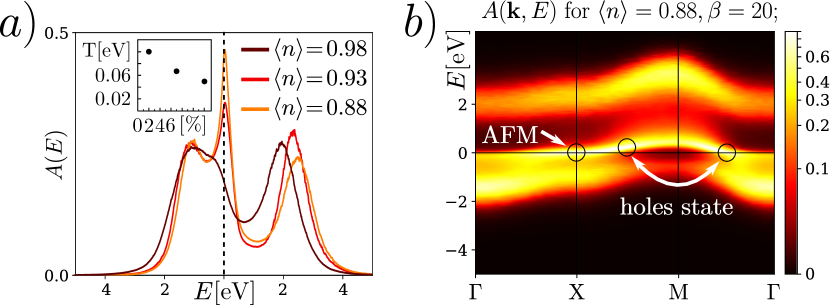
Figure 1: Single particle spectral function $A(E)$ of the extended Hubbard model for cuprates (a) is obtained for the different values of the hole-doping 2, 7 and 12 % for $\beta=10$, 15, and 20 eV^-1, respectively. With the increase of the doping it reveals a sharp peak at the Fermi energy, which corresponds to the existence of the flat band in the momentum space representation of the quasiparticle dispersion $A(\mathbf{k},E)$ (b), shown for $\left\langle n\right\rangle=0.88$. The inset in (a) shows points in the temperature T[eV] and doping [%] parameter space where calculations were performed.

As it is inherent in the Mott insulator, the energy spectrum of the undoped model for cuprates reveals two separated peaks (Hubbard sub-bands) that are located below and above the Fermi energy (see Fig. 1 a) and SM ). Upon small doping of $\sim 2\,\%$, the two-peak structure of the single-particle spectral function transforms to the three-peak structure, where the additional quasiparticle resonance appears at the Fermi level splitting off from the lower Hubbard band. The further increase of the doping to 7 and 12 % leads to an increase of the quasiparticle peak, which indicates the presence of a flat band in the quasiparticle dispersion where excessive charge carriers live (see Fig. 1 b). Remarkably, after the quasiparticle peak appears at the Fermi energy, the flat band at the anti-nodal point $\text{X}=(\pi,0)$ is pinned to the Fermi level and does not shift anymore with the further increase of the doping. This result is similar to previous theoretical studies of high-T_c cuprates PhysRevLett.89.076401 and Hubbard model on the triangular lattice PhysRevLett.112.070403 , where the case of the van Hove singularity at the Fermi level was considered. Apart from the pinning of the Fermi level, we observe that the hole-doping causes the reconstruction of the Fermi surface, which manifests itself in the flattening of the energy band at the vicinity of the ${\rm M}\Gamma/2=(\pi/2,\pi/2)$ nodal point. Redistribution of the spectral weight results in the increased density of holes that live around the X and ${\rm M}\Gamma/2$ points as depicted by white arrows in Fig. 1 b). The rest of the quasiparticle dispersion becomes very stable against doping due to strong correlation effects. Thus, the energy spectrum is shown here only for one particular case of $\left\langle n\right\rangle=0.88$. The other cases of doping are considered in the Supplemental Material SM .

One can also calculate the effective mass renormalization of electrons as $\varepsilon^{*}_{\mathbf{k}}=Z^{-1}\varepsilon_{\mathbf{k}}$ PhysRevB.62.R9283 for different values of doping discussed above. Here, $\varepsilon_{\mathbf{k}}$ is the Fourier transform of the hopping matrix parameterized by $t$ and $t^{\prime}$. It can be found that in the region close to the magnetic instability the system reveals almost the same renormalization coefficient $Z=4.7\pm 0.2$ SM for different dopings 2 %, 7 % and 12 %, which additionally confirms the fact that the quasiparticle dispersion becomes stable after it is pinned to the Fermi level. Note that our result for the mass renormalization qualitatively coincides with the experimental value observed in dahm2009strength ; Putzkee1501657 for another cuprate compound.

Now let us proceed to the two-particle description of the problem and look at the low-energy part of the momentum resolved magnetic susceptibility of the model shown in Fig. 2 b). Remarkably, the obtained dispersion of paramagnons does not change with doping and only reveals progressive broadening with an increase of the number of holes in the system SM similarly to what has been observed in a recent experiment PhysRevB.97.155144 . Another distinctive feature of the magnetic spectrum that is fortunately captured by the DB method is the high intensity at the $\text{M}=(\pi,\pi)$ point. This mode is associated with collective AFM fluctuations and is stable against the hole-doping with the maximum at the corresponding energies $E_{\rm max}=64\pm 3$ meV SM . Since specified small differences in the spin fluctuation spectrum are almost indistinguishable, the result for the magnetic susceptibility is shown in Fig. 2 b) only for one case of $\left\langle n\right\rangle=0.88$. Taking into account that the presence of doping usually destroys the ordering in the system, the result for the magnon dispersion looks counterintuitive at first glance. In order to get deeper understanding of this fact, one can look at the cut of the magnetic susceptibility at the maximum energy $E_{\rm max}$ shown in Fig 2 a) for different values of doping. Then, it becomes immediately clear that instead of breaking the AFM ordering, which corresponds here to the high peak at the M point, the conducting holes prefer to form their own magnetic state that appears as the second peak at the $\Gamma\text{X}/2=(\pi/2,0)$ point. Importantly, the height of the minor peak grows with the hole-doping, which explains the fact that the AFM mode stays in “resonance” and does not suffer from the existence of the excessive charge carriers in the system. A similar momentum-dependent variation of the spectral weight of spin fluctuations with doping was also reported in PhysRevB.97.155144 . The observed picture with no shift of the AFM intensity from the M point to an incommensurate position is consistent with the scenario of phase separation between the insulating AFM state and conducting droplets formed by the excessive charge carriers Auslender1982 ; nagaev1983physics .

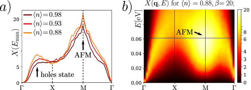
Figure 2: Momentum resolved magnetic susceptibility of the doped extended Hubbard model for cuprates (b) and its cut (a) at the energy $E_{\max}$ that corresponds to a maximum intensity at the M point. The corresponding value of the $E_{\max}$ is almost unchanged and for different hole-doping is $67$ meV (2 %), $66$ meV (7 %) and $61$ meV (12 %). The cut of the magnetic susceptibility reveals two-peaks that correspond to an AFM ordering (M-point) and magnetic holes state ($\Gamma\text{X}/2=(0,\pi/2)$ point).

Remarkably, the presence of the observed spin excitations in the doped extended Hubbard model for cuprates is reflected in the single-particle spectrum. It is known that in the undoped regime of the Mott insulator AFM fluctuations are governed by Anderson’s “superexchange” mechanism PhysRev.115.2 . Contrarily, in the doped case when the quasiparticle band lies at the Fermi energy the AFM spin fluctuation arise due to collective excitations of electrons between the anti-nodal $\text{X}=(\pi,0)$ and $\text{Y}=(0,\pi)$ points PhysRevLett.89.076401 ; PhysRevLett.112.070403 . This fact is also confirmed by the obtained energy spectrum (see Fig. 1 b)), where the high intensity at the Fermi level corresponds to the large density of the charge carriers that live at the vicinity of the X point as depicted by the small white arrow. Apart from the main AFM fluctuations, the presence of another region of high density of holes, appearing at the vicinity of the $\text{M}\Gamma/2=(\pi/2,\pi/2)$ point, allows an additional magnetic excitation of charge carriers between these two regions as shown by the white curved arrow. This excitation corresponds to the magnetic holes state shown in Fig. 2 a). Obviously, it is hard to distinguish only two peculiar points of the single-particle spectrum with states above and below the Fermi level that give the main contribution to the specified magnetic excitation, since the spectrum is broadened due to the presence of the large imaginary part of the electronic self-energy. Therefore, there is more than one pair of points that contribute to the magnetic holes state, which is also confirmed by the fact that the corresponding peak in Fig. 2 a) is relatively wide. However, the momentum space position of the latter allows to estimate the momentum difference between two areas of the single-particle spectrum that are responsible for this magnetic excitation. Looking back at the highest intensity points of the quasiparticle spectrum, one can conclude that the observed minor peak at the $\Gamma\text{X}/2=(\pi/2,0)$ point in the Fig. 2 a) indicates that this excitation happens roughly between the $\text{M}\Gamma/2$ and $\text{XM}/2=(\pi,\pi/2)$ points of the single-particle energy spectrum. Therefore, the redistribution of the quasiparticle weight in addition to the pinning of the quasiparticle spectrum to the Fermi energy allows to keep the single-particle energy spectrum stable against doping, which, in turn, is reflected in the unchanged magnon dispersion.

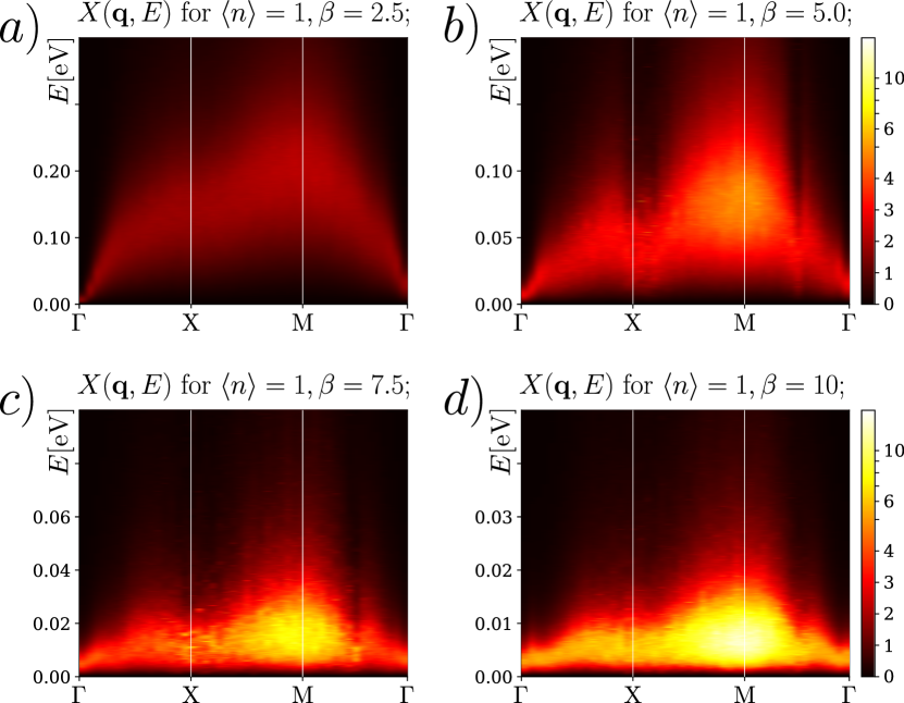
Figure 3: Momentum resolved magnetic susceptibility for the cuprate model for $\beta=2.5$ eV^-1 (a), 5.0 eV^-1 (b), 7.5 eV^-1 (c) and 10 eV^-1 (d). Intensity at the $\text{M}=(\pi,\pi)$ point corresponds to the formation of the AFM ordering and takes the maximum value at the energy $E_{\max}=219,\,90,\,18\,\text{and}\,9$ meV, respectively. The latter decreases when approaching the phase transition.

Since our modern approach allows to capture the fingerprint of the AFM ordering already in the paramagnetic phase near the leading magnetic instability, one can go deeper into the PM phase in order to observe the incipience of this fluctuation. Fig. 3 shows the momentum resolved low-energy part of the magnetic susceptibility of the undoped model for different temperatures. The Fig. 3 a) corresponds to the case of high temperature ($\beta=2.5$ eV^-1) and shows a standard paramagnon dispersion. Lowering the temperature to $\beta=5$ eV^-1, the characteristic energy scale of spin excitations decreases and the intensity at the M point of the magnon spectrum arises at the energy $E_{\max}=90$ meV (see Fig. 3 b)). Since the corresponding energy of the AFM fluctuations is proportional to the inverse of the spin correlation length, it decreases with the temperature as shown in the Fig. 3 c) ($\beta=7.5$ eV^-1) and goes almost to zero approaching the transition temperature at $\beta\simeq 10$ eV^-1 ($\lambda=0.96$) as shown in Fig. 3 d). Thus, it can be concluded that the antiferromagnetic mode that forms the ground state of the system in the ordered phase does not appear spontaneously below the transition temperature. On the contrary, it is developed at the finite energy well above the critical temperature already in the paramagnetic phase and “softens” approaching the phase boundary, which was also predicted in previous studies (see Ref. PhysRevB.60.1082 and references therein).

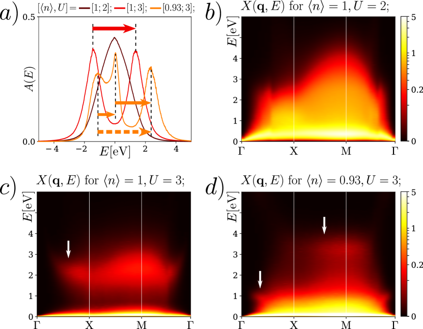
Figure 4: Single particle spectral function (a) and momentum resolved magnetic susceptibility in the strongly-correlated metallic $\left\langle n\right\rangle=1$, $U=2$ eV, $\beta=5$ eV^-1 (b); Mott-insulating $\left\langle n\right\rangle=1$, $U=3$ eV, $\beta=5$ eV^-1 (c); and doped Mott-insulating $\left\langle n\right\rangle=0.93$, $U=3$ eV, $\beta=15$ eV^-1 (d) regimes. In addition to the main low-lying mode of the high intensity, the magnon spectrum reveals additional one (c) and two (d) less pronounced high-energy bands that originate from the magnetic excitations between the corresponding peaks in the single particle spectral function depicted by the arrows in the top left panel. Energy $E$ is given in the units of eV.

Collective spin excitations of the Mott-insulator that are usually described theoretically are dispersive magnetic excitations that correspond either to the Anderson “superexchange” mechanism (in the undoped case), or to the collective electronic processes between the anti-nodal points of the quasiparticle band that lies at the Fermi energy (in the doped case) as discussed above. The characteristic energy of these excitations is of the order of the exchange interaction. In the most general case spin fluctuations are not restricted only to the low-energy magnon band and may reveal additional magnetic excitations. The latter have a completely different energy scale (of the order of the Coulomb interaction in the undoped case) and correspond to the electronic processes between peaks (sub-bands) of the single-particle spectral function. Moreover, they cannot be captured by the most of known theoretical approaches, since they are much less intense than the “usual” low-energy ones.

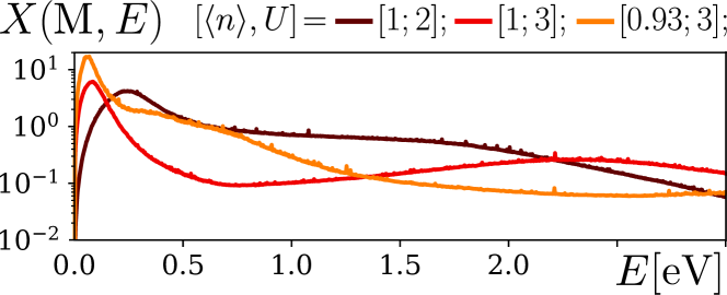
Figure 5: The cut of the momentum resolved magnetic susceptibility shown in Figs. 4 b)-d) at the M point as the function of the energy. The result is presented in the logarithmic scale.

In order to study the full spectrum of magnetic fluctuations, let us distinguish three cases of interest. First of all, it is worth noting that the considered model for cuprate compounds lies in the region close to the Mott insulator to metal phase transition. Reducing the local Coulomb interaction by $1$ eV ($U=2$ eV, $\left\langle n\right\rangle=1$) gives rise to a single peak in the single particle spectral function $A(E)$ in Fig. 4 a) shifting the material to a metal state. In addition, one can specify two more cases ($\left\langle n\right\rangle=1$ and $\left\langle n\right\rangle=0.93$) where the $A(E)$ of the extended Hubbard model for cuprates ($U=3$eV) has a two- and three-peak structure, respectively. Corresponding results for the momentum resolved magnetic susceptibility shown in Fig. 4 reveal one (b), two (c) and three (d) magnon bands. The less pronounced high-energy bands in Figs. 4 c) and d) are marked by white arrows. These additional bands originate from collective excitations between the specified peaks in the single particle spectral function, as depicted by arrows in the Fig. 4 a), similarly to the case of charge fluctuations PhysRevLett.113.246407 . It is worth mentioning that the process shown in Fig. 4 a) by the dashed arrow is suppressed, because it occurs between the most distant peaks and does not involve spin excitations from the Fermi level, contrary to the other two cases. Therefore, the corresponding magnon band is not observed in Fig. 4 d). For clarity, the cut of the magnetic susceptibility at the M point is shown in Fig. 5. The value of $X(\mathbf{q}$=M, $E)$ is given in a logarithmic scale in order to distinguish higher-energy bands from the intensive low-energy mode. Remarkably, the energy scale of these additional magnon bands coincides with the RIXS data obtained, for example, in Refs. Ghiringhelli1223532 ; guarise2014anisotropic for another cuprate compound. Unfortunately, the RIXS experiment cannot distinguish between the charge and spin excitations in the high-energy inter-band transitions. Therefore, the corresponding peak shown in these works contains both charge and spin fluctuations, and has the highest amplitude. Thus, the advanced DB scheme allows to capture the higher-energy transitions that are much less intensive than the lower-energy magnon band and to distinguish them from the charge excitations. To our knowledge, the existence of these high-energy magnetic excitations is reported in the literature for the first time.

II Conclusions

To summarize, in this work electronic properties of the doped extended Hubbard model for cuprate compounds in the paramagnetic phase close to the leading magnetic instability have been considered. Following the evolution of the electronic band structure of cuprates, we have observed that an additional quasiparticle band appears at the Fermi level already at the small values of doping. Further increase of doping leads to additional flattening of the energy band at the vicinity of the nodal $\text{M}\Gamma/2$ point and pinning the Fermi level to the anti-nodal points of the quasiparticle band. The redistribution of the quasiparticle density results in the spectral weight transfer to the vicinity of X (Y) and $\text{M}\Gamma/2$ points, which allows the observation of two magnetic modes in the spin fluctuation spectrum. Thus, collective electronic excitations between the anti-nodal X and Y points form the famous antiferromagnetic “resonant” mode, which remains unchanged in a broad range of temperatures and dopings. We have shown that protection of the AFM resonance is realized simultaneously through the pinning of the quasiparticle dispersion to the Fermi energy, and formation of another mode, which grows with doping and is located at the $\Gamma\text{X}/2$ point in the magnon spectrum. We have discovered that this mode corresponds to collective excitations of excessive charge carriers between the nodal $\text{M}\Gamma/2$ and anti-nodal XM/2 points.

The use of the advanced Dual Boson technique allowed us to investigate spin fluctuations in a wide spectral range. Thus, the incipience of the low-energy AFM mode in the undoped model for cuprates is captured in the paramagnetic regime far from the PM to AFM phase transition. This mode softens when approaching the transition temperature and forms the AFM ground state in the broken symmetry phase. The study of higher-energy magnetic fluctuations revealed additional less pronounced magnon bands. We have found that these bands originate from the collective electronic transitions between sub-bands in the quasiparticle energy spectrum and can be captured in the resonant inelastic X-ray scattering experiments le2011intense ; Ghiringhelli1223532 ; guarise2014anisotropic ; PhysRevLett.119.097001 ; PhysRevB.97.155144 .

III methods

The problem of collective excitations in cuprates is addressed here using the Dual Boson theory Rubtsov20121320 ; PhysRevB.93.045107 . The magnetic susceptibility in the ladder DB approximation is given by the following relation PhysRevLett.121.037204

$$\left[X^{\rm ladd}_{\mathbf{q}\omega}\right]^{-1}=J^{\rm d}_{\mathbf{q}}+\Lambda+\left[X^{\rm DMFT}_{\mathbf{q}\omega}\right]^{-1},$$ (1)

where $X^{\rm DMFT}_{\mathbf{q}\omega}$ is the DMFT-like PhysRevLett.62.324 ; RevModPhys.68.13 magnetic susceptibility written in terms of the local two-particle irreducible four-point vertices and lattice Green’s functions. The latter is dressed only in the local self-energy and is given by the usual EDMFT relation PhysRevB.52.10295 ; PhysRevLett.77.3391 . The single- and two-particle spectral functions are obtained, respectively, from the lattice Green’s function and magnetic susceptibility by a stochastic optimization method for analytic continuation SOM ; PhysRevB.62.6317 . The details of calculations can be found in SM .

The effective mass renormalization $Z$ of electrons can be found as $\varepsilon^{\ast}_{\mathbf{k}}=Z^{-1}\varepsilon_{\mathbf{k}}$, where the coefficient $Z$ reads PhysRevB.62.R9283

$$Z=1-\left.\frac{d\Sigma_{E}}{dE}\right|_{E=0},$$ (2)

since in the ladder DB approximation the electronic self-energy $\Sigma_{E}$ does not depend on momentum $\mathbf{k}$. Importantly, the calculation of the renormalization coefficient does not require the analytical continuation procedure. The result for the electronic self-energy can be found in SM .

The data that support the findings of this study are available from the corresponding author upon reasonable request.

Authors thank Nigel Hussey for inspiring discussions. We also thank Hartmut Hafermann for providing the impurity solver HAFERMANN20131280 based on the ALPS libraries 1742-5468-2011-05-P05001 , and Erik van Loon, Friedrich Krien and Arthur Huber for the help with the Dual Boson implementation.

The Authors declare no Competing Financial or Non-Financial Interests.

All authors discussed the results and contributed to the preparation of the manuscript.

E.A.S. and M.I.K. would like to thank the support of NWO via Spinoza Prize and of ERC Advanced Grant 338957 FEMTO/NANO. Also, E.A.S. and M.I.K. acknowledge the Stichting voor Fundamenteel Onderzoek der Materie (FOM), which is financially supported by the Nederlandse Organisatie voor Wetenschappelijk Onderzoek (NWO). I.S.K. acknowledges support from U.S. Department of Energy, Office of Science via Grant No. DOE ER 46932. A.I.L. acknowledges support from the excellence cluster “The Hamburg Centre for Ultrafast Imaging - Structure, Dynamics and Control of Matter at the Atomic Scale” and North-German Supercomputing Alliance (HLRN) under the Project No. hhp00040. The contribution of A.I.L. and A.N.R. was funded by the joint Russian Science Foundation (RSF)/DFG Grant No. 16-42-01057 / LI 1413/9-1.

Supplemental Material for
Quantum spin fluctuations and evolution of electronic structure in cuprates

IV Action

The action of the considered extended Hubbard model written in momentum space has the following form

$${\cal S}=-\sum_{\mathbf{k},\nu,\sigma}c^{*}_{\mathbf{k}\nu\sigma}\left[i\nu+\mu-\varepsilon^{\phantom{*}}_{\mathbf{k}}\right]\,c^{\phantom{\dagger}}_{\mathbf{k}\nu\sigma}+U\sum\limits_{\mathbf{q},\omega}n^{*}_{\mathbf{q}\omega\uparrow}n^{\phantom{*}}_{\mathbf{q}\omega\downarrow}+\frac{1}{2}\sum\limits_{\mathbf{q},\omega,\varsigma}V^{\,\varsigma}_{\mathbf{q}}\rho^{*\,\varsigma}_{\mathbf{q}\omega}\,\rho^{\,\varsigma}_{\mathbf{q}\omega}.$$ (3)

Here, $c^{*}_{\mathbf{k}\nu\sigma}$ ($c_{\mathbf{k}\nu\sigma}$) are Grassmann variables corresponding to creation (annihilation) of an electron with momentum $\mathbf{k}$, fermionic Matsubara frequency $\nu$ and spin $\sigma$. $\varepsilon_{\mathbf{k}}$ is the Fourier transform of the nearest-neighbor (NN) $t$ and next-NN $t^{\prime}$ hopping amplitudes. The label $\varsigma=\{c,s\}$ depicts charge $c$ and spin $s=\{x,y,z\}$ degrees of freedom, so that $U$ and $V^{\,c}_{\mathbf{q}}=V_{\mathbf{q}}$ describe local and nonlocal parts of the Coulomb interaction respectively, and $V^{\,s}_{\mathbf{q}}=-J^{\rm d}_{\mathbf{q}}/2$ is the nonlocal direct ferromagnetic exchange interaction. Here, we also introduce bosonic variables $\rho^{\,\varsigma}_{\mathbf{q}\omega}=~{}n^{\,\varsigma}_{\mathbf{q}\omega}-~{}\left\langle n^{\,\varsigma}_{\mathbf{q}\omega}\right\rangle$, where $n^{\,\varsigma}_{\mathbf{q}\omega}=\sum_{\mathbf{k}\nu\sigma\sigma^{\prime}}c^{*}_{\mathbf{k}+\mathbf{q},\nu+\omega,\sigma}\sigma^{\,\varsigma}_{\sigma\sigma^{\prime}}c^{\phantom{*}}_{\mathbf{k},\nu,\sigma^{\prime}}$ is the charge (spin) density with momentum $\mathbf{q}$ and bosonic Matsubara frequency $\omega$ and $\sigma^{\,c\,(s)}=I\,(\sigma)$ is the unit (Pauli) matrix for the charge (spin) channels, respectively.

The description of collective excitations is given here within the ladder Dual Boson theory  Rubtsov20121320 ; PhysRevB.90.235135 ; PhysRevB.93.045107 ; PhysRevB.94.205110 , which implies exact solution of the corresponding local impurity problem

$${\cal S}_{\rm imp}= -\sum\limits_{\nu,\sigma}c^{*}_{\nu\sigma}\left[i\nu+\mu-\Delta^{\phantom{*}}_{\nu}\right]c^{\phantom{*}}_{\nu\sigma}+U\sum\limits_{\omega}n^{*}_{\omega\uparrow}n^{\phantom{*}}_{\omega\downarrow}+\frac{1}{2}\sum\limits_{\omega,\varsigma}\Lambda^{\,\varsigma}_{\omega}\,\rho^{*\,\varsigma}_{\omega}\,\rho^{\,\varsigma}_{\omega},$$ (4)

where the fermionic $\Delta_{\nu}$ and bosonic $\Lambda^{\varsigma}_{\omega}$ hybridization functions are introduced similarly to the EDMFT PhysRevB.52.10295 ; PhysRevLett.77.3391 ; PhysRevB.61.5184 ; PhysRevLett.84.3678 ; PhysRevB.63.115110 ; PhysRevLett.90.086402 in order to effectively account for nonlocal excitations and have to be determined self-consistently. Note that the same functions have to be excluded from the remaining nonlocal part of the action

$${\cal S}_{\rm rem}=-\sum\limits_{\mathbf{k},\nu,\sigma}c^{*}_{\mathbf{k}\nu\sigma}\left[\Delta^{\phantom{*}}_{\nu}-\varepsilon^{\phantom{*}}_{\mathbf{k}}\right]c^{\phantom{*}}_{\bf{k}\nu\sigma}+\frac{1}{2}\sum\limits_{\mathbf{q},\omega,\varsigma}\left(V^{\,\varsigma}_{\mathbf{q}}-\Lambda^{\,\varsigma}_{\omega}\right)\rho^{*\,\varsigma}_{\mathbf{q}\omega}\,\rho^{\,\varsigma}_{\mathbf{q}\omega},$$ (5)

so that the total lattice problem ${\cal S}=\sum_{i}{\cal S}^{(i)}_{\rm imp}+{\cal S}_{\rm rem}$ is unchanged. Inclusion of bosonic hybridization functions is important and leads to a great improvement of results already at the dynamical mean-field level PhysRevB.90.235135 ; PhysRevB.94.205110 . Nevertheless, this procedure has some hidden difficulties. As it was shown recently, while the bosonic hybridization function $\Lambda^{c}_{\omega}$ in the charge channel performs rather well, the account for the same kind of frequency dependent function $\Lambda^{s}_{\omega}$ in the spin channel leads to the changed Ward identity and thus breaks the local spin conservation at the impurity level PhysRevB.96.075155 . Also, the inclusion of the bosonic hybridization function in the spin channel drastically complicates solution of the impurity problem and is often associated with the sign problem. Whereas the solution of this issue in the single-band case was recently proposed PhysRevB.87.125102 , an application of this method to realistic multiorbital systems is extremely complicated and is not done yet. However, there is still one particular form of the bosonic hybridization function, which does not violate local conservation laws, stays almost undiscussed. Indeed, when the bosonic hybridization for the spin channel is approximated by a constant function in the frequency space $\Lambda^{s}_{\omega}\to\Lambda^{s}$, the local Ward identity remains unchanged and conservation laws are fulfilled .

V Variation of the impurity problem

The important consequence of introducing of retarded interactions is that every variation $\delta\Delta_{\nu}$ and $\delta\Lambda_{\omega}^{\,\varsigma}$ doesn’t change the total action and, as a consequence, the partition function. It is also possible to vary retarded interactions in such a way that the impurity problem (4) remains unchanged as well. According to above discussions, let us assume that $\delta\Delta$ and $\delta\Lambda^{\,\varsigma}$ are constant variations of fermionic and bosonic hybridization functions. Therefore, the variation of the impurity action reads

$$2\,\delta{\cal S}_{\rm imp} =2\,\delta\Delta\sum_{\nu\sigma}c^{*}_{\nu\sigma}c^{\phantom{*}}_{\nu\sigma}+\delta\Lambda^{c}\sum_{\omega}\rho^{*\,c}_{\omega}\,\rho^{\,c}_{\omega}+\delta\Lambda^{s}\sum\limits_{s,\omega}\rho^{*\,s}_{\omega}\,\rho^{\,s}_{\omega}.$$ (6)

$$=2\,\delta\Delta\sum_{\nu\sigma}c^{*}_{\nu\sigma}c^{\phantom{*}}_{\nu\sigma}+2\,\delta\Lambda^{c}\sum_{\omega}n^{*}_{\omega\uparrow}n^{\phantom{*}}_{\omega\downarrow}-\delta\Lambda^{c}\sum_{\nu\sigma}c^{*}_{\nu\sigma}c^{\phantom{*}}_{\nu\sigma}+\delta\Lambda^{c}\left\langle n\right\rangle-6\,\delta\Lambda^{s}\sum\limits_{\omega}n^{*}_{\omega\uparrow}n^{\phantom{*}}_{\omega\downarrow}+\delta\Lambda^{s}\sum_{\nu\sigma}c^{*}_{\nu\sigma}c^{\phantom{*}}_{\nu\sigma}$$

$$=\Big{(}2\,\delta\Delta-\delta\Lambda^{c}+\delta\Lambda^{s}\Big{)}\sum_{\nu\sigma}c^{*}_{\nu\sigma}c^{\phantom{*}}_{\nu\sigma}+2\,\Big{(}\delta\Lambda^{c}-3\delta\Lambda^{s}\Big{)}\sum_{\omega}n^{*}_{\omega\uparrow}n^{\phantom{*}}_{\omega\downarrow}+\delta\Lambda^{c}\left\langle n\right\rangle,$$

where we considered an anisotropic case of spin fluctuations $\delta\Lambda^{x}=\delta\Lambda^{y}=\delta\Lambda^{z}=\delta\Lambda^{s}$. Since the impurity problem is assumed to be unchanged under these transformations, one gets the following relations for the introduced variations

$$\delta\Lambda^{c}=3\,\delta\Lambda^{s},$$ (7)

$$\delta\Delta=\frac{\delta\Lambda^{c}-\delta\Lambda^{s}}{2}=\delta\Lambda^{s}.$$ (8)

Here, the last relation describes a constant shift of the chemical potential $\mu$. Thus, the total variation of the impurity action is

$$\delta{\cal S}_{\rm imp}=\delta\Lambda^{c}\left\langle n\right\rangle/2,$$ (9)

which is just a constant shift of the energy that does not affect the calculation of local observables. Then, based on the above transformation, the initial action (4) of the impurity model can be simplified as

$${\cal S}_{\rm imp} =-\sum\limits_{\nu,\sigma}c^{*}_{\nu\sigma}\left[i\nu+\mu-\Delta^{\phantom{*}}_{\nu}\right]c^{\phantom{*}}_{\nu\sigma}+U\sum\limits_{\omega}n^{*}_{\omega\uparrow}n^{\phantom{*}}_{\omega\downarrow}+\frac{1}{2}\sum\limits_{\omega,\varsigma}\Lambda^{\,\varsigma}_{\omega}\,\rho^{*\,\varsigma}_{\omega}\,\rho^{\,\varsigma}_{\omega},$$ (10)

$$=-\sum\limits_{\nu,\sigma}c^{*}_{\nu\sigma}\left[i\nu+\mu-\Delta_{\nu}\right]c^{\phantom{*}}_{\nu\sigma}+U\sum_{\omega}n^{*}_{\omega\uparrow}n^{\phantom{*}}_{\omega\downarrow}+\frac{1}{2}\sum\limits_{\omega}\left[\Lambda^{c}_{\omega}-3\Lambda^{s}\right]\rho^{*\,c}_{\omega}\rho^{\,c}_{\omega}-\Lambda^{s}\sum_{\nu\sigma}c^{*}_{\nu\sigma}c^{\phantom{*}}_{\nu\sigma}$$

$$=-\sum\limits_{\nu,\sigma}c^{*}_{\nu\sigma}\left[i\nu+\tilde{\mu}-\Delta_{\nu}\right]c^{\phantom{*}}_{\nu\sigma}+U\sum_{\omega}n^{*}_{\omega\uparrow}n^{\phantom{*}}_{\omega\downarrow}+\frac{1}{2}\sum\limits_{\omega}\Lambda^{0}_{\omega}\,\rho^{*\,c}_{\omega}\,\rho^{\,c}_{\omega},$$

where $\delta\Lambda^{s}=-\Lambda^{s}$, $\tilde{\mu}=\mu+\Lambda^{s}$ and $\Lambda^{0}=\Lambda^{c}_{\omega}-3\Lambda^{s}$.

If the charge hybridization function is also taken as a constant $\Lambda^{c}_{\omega}=\Lambda^{c}$, then the action (10) simplifies to

$${\cal S}_{\rm imp}=-\sum\limits_{\nu,\sigma}c^{*}_{\nu\sigma}\left[i\nu+\mu^{\prime}-\Delta_{\nu}\right]c^{\phantom{*}}_{\nu\sigma}+U^{\prime}\sum_{\omega}n^{*}_{\omega\uparrow}n^{\phantom{8}}_{\omega\downarrow},$$ (11)

where $\mu^{\prime}=\mu+(\Lambda^{c}-\Lambda^{s})/2$ and $U^{\prime}=U+\Lambda^{c}-3\Lambda^{s}$.

Therefore, all local observables of impurity model (4) can be calculated using simpler local problems written in the EDMFT (10) and DMFT (11) forms. It turns out that this approximation is very attractive for numerical calculations, since the inclusion of the spin channel in the impurity problem (4) does not require additional implementation, since the simplified actions (10) and (11) contain only the charge degrees of freedom.

VI Variation of the lattice problem

The partition function of the initial problem is given by the following relation

$${\cal Z}=\int D[c]\,e^{-{\cal S}}.$$ (12)

According to the usual formulation of the Dual Boson theory Rubtsov20121320 ; PhysRevB.90.235135 ; PhysRevB.93.045107 ; PhysRevB.94.205110 , one can perform Hubbard–Stratonovich transformations of the nonlocal part of the action ${\cal S}_{\rm rem}$ and introduce new ${\it dual}$ variables $f^{*},f,\phi^{\,\varsigma}$ as

$$\exp\left\{\,\sum\limits_{{\bf k}\nu\sigma}c^{*}_{{\bf k}\nu\sigma}[\Delta_{\nu\sigma}-\varepsilon_{\bf k}]c^{\phantom{*}}_{{\bf k}\nu\sigma}\right\} ={\cal D}_{f}\int D[f]\,\exp\left\{-\sum\limits_{{\bf k}\nu\sigma}\left(f^{*}_{{\bf k}\nu\sigma}[\Delta_{\nu\sigma}-\varepsilon_{\bf k}]^{-1}f^{\phantom{*}}_{{\bf k}\nu\sigma}+c^{*}_{\nu\sigma}f^{\phantom{*}}_{\nu\sigma}+f^{*}_{\nu\sigma}c^{\phantom{*}}_{\nu\sigma}\right)\right\},$$

$$\exp\left\{\,\frac{1}{2}\sum\limits_{\mathbf{q}\omega}\rho^{*\,\varsigma}_{{\bf q}\omega}[\Lambda^{\,\varsigma}_{\omega}-V^{\,\varsigma}_{\mathbf{q}}]\rho^{\,\varsigma}_{\mathbf{q}\omega}\right\} ={\cal D}_{\varsigma}\int D[\phi^{\,\varsigma}]\,\exp\left\{-\frac{1}{2}\sum\limits_{\mathbf{q}\omega}\left(\phi^{*\,\varsigma}_{\mathbf{q}\omega}[\Lambda^{\,\varsigma}_{\omega}-V^{\,\varsigma}_{\mathbf{q}}]^{-1}\phi^{\,\varsigma}_{\mathbf{q}\omega}+\rho^{*\,\varsigma}_{\omega}\phi^{\,\varsigma}_{\omega}+\phi^{*\,\varsigma}_{\omega}\rho^{\,\varsigma}_{\omega}\right)\right\},$$

where ${\cal D}_{f}={\rm det}[\Delta_{\nu\sigma}-\varepsilon_{\bf k}]$ and ${\cal D}^{-1}_{\,\varsigma}=\mkern-6.0mu\mathop{}\sqrt[\mkern 8.0mu]{{\rm det}[\Lambda^{\varsigma}_{\omega}-V^{\,\varsigma}_{\bf q}]}$. Rescaling the fermionic field as $f_{{\bf k}\nu\sigma}\to{}f_{{\bf k}\nu\sigma}g^{-1}_{\nu\sigma}$ and bosonic field as $\phi^{\,\varsigma}_{\mathbf{q}\omega}\to{}\phi^{\,\varsigma}_{\mathbf{q}\omega}\alpha^{\,\varsigma~{}-1}_{\omega}$, we transform the initial problem (4) to ${\cal S}=\sum_{i}{\cal S}^{(i)}_{\rm imp}+{\cal S}_{\rm DB}$, where

$${\cal S}_{\rm DB}= -\sum_{\mathbf{k},\nu,\sigma}f^{*}_{\mathbf{k}\nu\sigma}g^{-1}_{\nu\sigma}(\varepsilon_{\mathbf{k}}-\Delta_{\nu})^{-1}g^{-1}_{\nu\sigma}f^{\phantom{*}}_{\mathbf{k}\nu\sigma}+\sum_{\mathbf{k},\nu,\sigma}\left[c^{*}_{\mathbf{k}\nu\sigma}g^{-1}_{\nu\sigma}f^{\phantom{*}}_{\mathbf{k}\nu\sigma}+f^{*}_{\mathbf{k}\nu\sigma}g^{-1}_{\nu\sigma}c^{\phantom{*}}_{\mathbf{k}\nu\sigma}\right]$$

$$-\frac{1}{2}\sum_{\mathbf{q},\omega,\varsigma}\phi^{*\,\varsigma}_{\mathbf{q}\omega}\alpha^{\,\varsigma~{}-1}_{\omega}(V^{\,\varsigma}_{\mathbf{q}}-\Lambda^{\varsigma}_{\omega})^{-1}\alpha^{\,\varsigma~{}-1}_{\omega}\phi^{\,\varsigma}_{\mathbf{q}\omega}+\frac{1}{2}\sum_{\mathbf{q},\omega}\left[\rho^{*\,\varsigma}_{\mathbf{q}\omega}\alpha^{\,\varsigma~{}-1}_{\omega}\phi^{\,\varsigma}_{\mathbf{q}\omega}+\phi^{*\,\varsigma}_{\mathbf{q}\omega}\alpha^{\,\varsigma~{}-1}_{\omega}\rho^{\,\varsigma}_{\mathbf{q}\omega}\right].$$

Let us now consider same variations of the lattice problem

$$\frac{\delta{\cal Z}}{\cal Z} =\frac{1}{\cal Z}\,\delta\left[{\cal D}_{f}{\cal D}_{c}{\cal D}_{s}\int D[c,f,\phi^{c},\phi^{s}]\,e^{-{\cal S}_{\rm DB}}e^{-\sum_{i}{\cal S}^{(i)}_{\rm imp}}\right]$$ (13)

$$=\frac{\delta{}{\cal D}_{f}}{{\cal D}_{f}}+\frac{\delta{}{\cal D}_{c}}{{\cal D}_{c}}+\frac{\delta{}{\cal D}_{s}}{{\cal D}_{s}}+\frac{{\cal D}_{f}{\cal D}_{c}{\cal D}_{s}}{\cal Z}\int D[c,f,\phi^{c},\phi^{s}]\left[-\delta{}{\cal S}_{\rm DB}\right]e^{-{\cal S}}+\frac{{\cal D}_{f}{\cal D}_{c}{\cal D}_{s}}{\cal Z}\int D[c,f,\phi^{c},\phi^{s}]\left[-\sum\limits_{i}\delta{}{\cal S}^{i}_{\rm imp}\right]e^{-{\cal S}}$$

that do not change the partition function ${\cal Z}$ as discussed above. Since the previously obtained total variation of the impurity action is $\delta{\cal S}_{\rm imp}=\delta\Lambda^{c}\left\langle n\right\rangle/2$, one gets the following expression

$$0=\delta\Lambda^{c}\left\langle n\right\rangle +2\delta\Delta\sum_{\mathbf{k},\nu,\sigma}\left\{\left[\Delta_{\nu\sigma}-\varepsilon_{\mathbf{k}}\right]^{-1}g^{-1}_{\nu\sigma}\left\langle f^{*}_{\mathbf{k}\nu\sigma}f^{\phantom{*}}_{\mathbf{k}\nu\sigma}\right\rangle_{\rm latt}g^{-1}_{\nu\sigma}\left[\Delta_{\nu\sigma}-\varepsilon_{\mathbf{k}}\right]^{-1}-\left[\Delta_{\nu\sigma}-\varepsilon_{\mathbf{k}}\right]^{-1}\right\}$$

$$+\delta\Lambda^{c}\sum_{\mathbf{q},\omega}\left\{\left[\Lambda^{c}_{\omega}-V_{\mathbf{q}}^{c}\right]^{-1}\alpha^{-1\,c}_{\omega}\left\langle\phi^{*\,c}_{\mathbf{q}\omega}\phi^{c}_{\mathbf{q}\omega}\right\rangle_{\rm latt}\alpha^{-1\,c}_{\omega}\left[\Lambda^{c}_{\omega}-V_{\mathbf{q}}^{c}\right]^{-1}-\left[\Lambda^{c}_{\omega}-V_{\mathbf{q}}^{c}\right]^{-1}\right\}$$

$$+\delta\Lambda^{s}\sum_{\mathbf{q},\omega,s}\left\{\left[\Lambda^{s}_{\omega}-V_{\mathbf{q}}^{s}\right]^{-1}\alpha^{-1\,s}_{\omega}\left\langle\phi^{*\,s}_{\mathbf{q}\omega}\phi^{s}_{\mathbf{q}\omega}\right\rangle_{\rm latt}\alpha^{-1\,s}_{\omega}\left[\Lambda^{s}_{\omega}-V_{\mathbf{q}}^{s}\right]^{-1}-\left[\Lambda^{s}_{\omega}-V_{\mathbf{q}}^{s}\right]^{-1}\right\}.$$ (14)

Using the exact relation between the lattice and dual quantities Rubtsov20121320 ; PhysRevB.90.235135 ; PhysRevB.93.045107 ; PhysRevB.94.205110 and connections between variations of hybridization functions (7) and (8), one gets the following analytical expression for the “Pauli principle”

$$3\sum_{\mathbf{q},\omega}X^{c}_{\mathbf{q}\omega}+\sum_{\mathbf{q},\omega,s}X^{s}_{\mathbf{q}\omega} =3\left\langle n\right\rangle-2\sum_{\mathbf{k},\nu,\sigma}G_{\mathbf{k}\nu\sigma}=\left\langle n\right\rangle.$$ (15)

Here $X_{\mathbf{q}\omega}$ and $\chi_{\omega}$ are the lattice and impurity susceptibilities, respectively. Therefore, if one takes the

$$\sum_{\mathbf{q},\omega}X^{\varsigma}_{\mathbf{q}\omega}=\sum_{\omega}\chi^{\varsigma}_{\omega}$$ (16)

self-consistency condition on the hybridization function $\Lambda^{\varsigma}$, the “Pauli principle” is fulfilled automatically, because the impurity problem is solved numerically exactly and the following relation

$$3\sum_{\omega}\chi^{c}_{\omega}+\sum_{s,\omega}\chi^{s}_{\omega} =\left\langle n\right\rangle$$ (17)

is correct by definition.

VII Calculation of observables

All lattice quantities of the considered problem can be obtained following the standard Dual Boson scheme Rubtsov20121320 ; PhysRevB.90.235135 ; PhysRevB.93.045107 ; PhysRevB.94.205110 with the only one difference in the self-consistency condition (16) on the constant bosonic hybridization function $\Lambda^{\varsigma}$. In our work we restrict ourselves to the ladder Dual Boson description of collective excitations. Therefore, the lattice self-energy $\Sigma_{\mathbf{k}\nu\sigma}$ is approximated by that of the local impurity problem (4) and the nonlocal contribution is omitted in order to obey charge and spin conservation laws. Then, the lattice Green’s function is equal to the EDMFT Green’s function $G_{\mathbf{k}\nu\sigma}$ and the magnetic susceptibility can be written in the following form PhysRevLett.121.037204

$$\left[X^{\rm ladd}_{\mathbf{q}\omega}\right]^{-1}=J^{\rm d}_{\mathbf{q}}+\Lambda+\left[X^{\rm DMFT}_{\mathbf{q}\omega}\right]^{-1},$$ (18)

where $X^{\rm DMFT}_{\mathbf{q}\omega}$ is the DMFT-like PhysRevLett.62.324 ; RevModPhys.68.13 magnetic susceptibility written in terms of the local two-particle irreducible four-point vertices and lattice Green’s functions. Numerical calculations of the Green’s function and susceptibility are performed on the $32\times 32$ lattice. Number of $\bf{k}$ points in the Brillouin Zone is the same as for the lattice sites, namely $32\times 32$. Number of fermionic Matsubara frequencies is 36, which is twice larger than the bosonic one. The single- and two-particle spectral functions are shown in Fig. 6 and Fig. 8, respectively, and obtained from the lattice Green’s function and magnetic susceptibility by the stochastic optimization method for analytic continuation SOM ; PhysRevB.62.6317 .

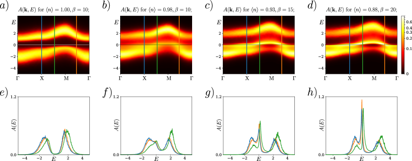
Figure 6: Evolution of the energy spectrum $A(\mathbf{q},E)$ of the La₂CuO₄ (top row) and its cut at X, XM/2 and $\text{M}\Gamma/2$ (bottom row) obtained in the paramagnetic regime close to the PM to AFM phase boundary for different values of hole-doping (from left to right) $\left\langle n\right\rangle=1$, 0.98, 0.93, and 0.88, respectively. The energy $E$ is given in the units of eV.

The evolution of the electronic band structure of cuprates with the hole-doping is shown in Fig. 6 a)-d). One can observe that already at small hole-doping of 2 %, the two-peak structure of the single-particle spectral function formed by the lower and upper Hubbard bands transforms to the three-peak structure, where the additional quasiparticle resonance appears at the Fermi level splitting off from the lower Hubbard band. The further increase of the doping to $\left\langle n\right\rangle=0.93$ and $\left\langle n\right\rangle=0.88$ leads to the additional flattening of the quasiparticle band at the vicinity of the nodal $\text{M}\Gamma/2$ point and pinning of the Fermi level to the nodal and anti-nodal points of the energy spectrum. The redistribution of the quasiparticle density upon doping results in sharp peaks and almost identical behavior of the electronic density at the X and $\text{M}\Gamma/2$ points as shown in Fig. 6 e)-h). The corresponding result for the electronic self-energy is presented in the Fig 7.

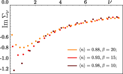
Figure 7: Imaginary part of the electronic self-energy for the extended Hubbard model for cuprates in the Matsubara frequency representation obtained in the paramagnetic regime close to the PM to AFM phase boundary for different values of hole-doping $\left\langle n\right\rangle=0.98$, 0.93 and 0.88. The energy and Matsubara frequencies are given in the eV.

Fig. 8 shows the magnon spectrum as a function of hole-doping. As one can see, the obtained dispersion of paramagnons is almost unchanged with doping and only reveals progressive broadening with the increase of number of holes. The high intensity at the M point has the maximum at the corresponding energies $E_{\rm max}=67$ meV ($\left\langle n\right\rangle=0.98$), $66$ meV ($\left\langle n\right\rangle=0.93$) and $61$ meV ($\left\langle n\right\rangle=0.88$) and is associated with collective AFM fluctuations.

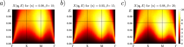
Figure 8: Momentum resolved magnetic susceptibility of the cuprate model obtained in the paramagnetic regime close to the PM to AFM phase boundary for different values of hole-doping (from left to right) $\left\langle n\right\rangle=0.98$, $\left\langle n\right\rangle=0.93$ and $\left\langle n\right\rangle=0.88$. The energy $E$ is given in the eV.

References

- (1) Anderson, P. W. Is There Glue in Cuprate Superconductors? Science 316, 1705–1707 (2007). URL http://science.sciencemag.org/content/316/5832/1705.
- (2) Dagotto, E. Correlated electrons in high-temperature superconductors. Rev. Mod. Phys. 66, 763–840 (1994). URL https://link.aps.org/doi/10.1103/RevModPhys.66.763.
- (3) Scalapino, D. J. A common thread: The pairing interaction for unconventional superconductors. Rev. Mod. Phys. 84, 1383–1417 (2012). URL https://link.aps.org/doi/10.1103/RevModPhys.84.1383.
- (4) Irkhin, V. Y., Katanin, A. A. & Katsnelson, M. I. Self-consistent spin-wave theory of layered Heisenberg magnets. Phys. Rev. B 60, 1082–1099 (1999). URL https://link.aps.org/doi/10.1103/PhysRevB.60.1082.
- (5) Mook, H. A., Yethiraj, M., Aeppli, G., Mason, T. E. & Armstrong, T. Polarized neutron determination of the magnetic excitations in . Phys. Rev. Lett. 70, 3490–3493 (1993). URL https://link.aps.org/doi/10.1103/PhysRevLett.70.3490.
- (6) Dai, P. et al. The Magnetic Excitation Spectrum and Thermodynamics of High-Tc Superconductors. Science 284, 1344–1347 (1999). URL http://science.sciencemag.org/content/284/5418/1344.
- (7) Bourges, P. et al. The Spin Excitation Spectrum in Superconducting YBa2Cu3O6.85. Science 288, 1234–1237 (2000). URL http://science.sciencemag.org/content/288/5469/1234.
- (8) Vignolle, B. et al. Two energy scales in the spin excitations of the high-temperature superconductor La2-xSrxCuO4. Nature Physics 3, 163–167 (2007).
- (9) Fujita, M. et al. Progress in Neutron Scattering Studies of Spin Excitations in High-Tc Cuprates. Journal of the Physical Society of Japan 81, 011007 (2012). URL https://doi.org/10.1143/JPSJ.81.011007.
- (10) Dahm, T. et al. Strength of the spin-fluctuation-mediated pairing interaction in a high-temperature superconductor. Nature Physics 5, 217–221 (2009).
- (11) Li, W.-J., Lin, C.-J. & Lee, T.-K. Signatures of strong correlation effects in resonant inelastic X-ray scattering studies on cuprates. Phys. Rev. B 94, 075127 (2016). URL https://link.aps.org/doi/10.1103/PhysRevB.94.075127.
- (12) Kung, Y. F. et al. Doping evolution of spin and charge excitations in the Hubbard model. Phys. Rev. B 92, 195108 (2015). URL https://link.aps.org/doi/10.1103/PhysRevB.92.195108.
- (13) Jia, C., Wohlfeld, K., Wang, Y., Moritz, B. & Devereaux, T. P. Using RIXS to Uncover Elementary Charge and Spin Excitations. Phys. Rev. X 6, 021020 (2016). URL https://link.aps.org/doi/10.1103/PhysRevX.6.021020.
- (14) Kanász-Nagy, M., Shi, Y., Klich, I. & Demler, E. A. Resonant inelastic X-ray scattering as a probe of band structure effects in cuprates. Phys. Rev. B 94, 165127 (2016). URL https://link.aps.org/doi/10.1103/PhysRevB.94.165127.
- (15) Hayden, S. M. et al. High-energy spin waves in . Phys. Rev. Lett. 67, 3622–3625 (1991). URL https://link.aps.org/doi/10.1103/PhysRevLett.67.3622.
- (16) Shimahara, H. & Takada, S. Fragility of the antiferromagnetic long-range-order and spin correlation in the two-dimensional tJ model. Journal of the Physical Society of Japan 61, 989–997 (1992).
- (17) Sega, I., Prelovšek, P. & Bonča, J. Magnetic fluctuations and resonant peak in cuprates: Towards a microscopic theory. Phys. Rev. B 68, 054524 (2003). URL https://link.aps.org/doi/10.1103/PhysRevB.68.054524.
- (18) Katanin, A. A. & Kampf, A. P. Spin excitations in Consistent description by inclusion of ring exchange. Phys. Rev. B 66, 100403 (2002). URL https://link.aps.org/doi/10.1103/PhysRevB.66.100403.
- (19) Pines, D. & Nozières, P. The Theory of Quantum Liquids: Normal Fermi liquids (W.A. Benjamin, Philadelphia, 1966).
- (20) Brinckmann, J. & Lee, P. A. Renormalized mean-field theory of neutron scattering in cuprate superconductors. Phys. Rev. B 65, 014502 (2001). URL https://link.aps.org/doi/10.1103/PhysRevB.65.014502.
- (21) Manske, D., Eremin, I. & Bennemann, K. H. Analysis of the resonance peak and magnetic coherence seen in inelastic neutron scattering of cuprate superconductors: A consistent picture with tunneling and conductivity data. Phys. Rev. B 63, 054517 (2001). URL https://link.aps.org/doi/10.1103/PhysRevB.63.054517.
- (22) Abanov, A., Chubukov, A. V., Eschrig, M., Norman, M. R. & Schmalian, J. Neutron Resonance in the Cuprates and its Effect on Fermionic Excitations. Phys. Rev. Lett. 89, 177002 (2002). URL https://link.aps.org/doi/10.1103/PhysRevLett.89.177002.
- (23) Jia, C. et al. Persistent spin excitations in doped antiferromagnets revealed by resonant inelastic light scattering. Nature communications 5, 3314 (2014).
- (24) White, S. R. et al. Numerical study of the two-dimensional Hubbard model. Phys. Rev. B 40, 506–516 (1989). URL https://link.aps.org/doi/10.1103/PhysRevB.40.506.
- (25) Loh, E. Y. et al. Sign problem in the numerical simulation of many-electron systems. Phys. Rev. B 41, 9301–9307 (1990). URL https://link.aps.org/doi/10.1103/PhysRevB.41.9301.
- (26) Sengupta, A. M. & Georges, A. Non-Fermi-liquid behavior near a T=0 spin-glass transition. Phys. Rev. B 52, 10295–10302 (1995). URL https://link.aps.org/doi/10.1103/PhysRevB.52.10295.
- (27) Si, Q. & Smith, J. L. Kosterlitz-Thouless Transition and Short Range Spatial Correlations in an Extended Hubbard Model. Phys. Rev. Lett. 77, 3391–3394 (1996). URL http://link.aps.org/doi/10.1103/PhysRevLett.77.3391.
- (28) Rohringer, G. et al. Diagrammatic routes to nonlocal correlations beyond dynamical mean field theory. Rev. Mod. Phys. 90, 025003 (2018). URL https://link.aps.org/doi/10.1103/RevModPhys.90.025003.
- (29) Rubtsov, A., Katsnelson, M. & Lichtenstein, A. Dual boson approach to collective excitations in correlated fermionic systems. Annals of Physics 327, 1320 – 1335 (2012). URL http://www.sciencedirect.com/science/article/pii/S0003491612000164.
- (30) Stepanov, E. A. et al. Self-consistent dual boson approach to single-particle and collective excitations in correlated systems. Phys. Rev. B 93, 045107 (2016). URL http://link.aps.org/doi/10.1103/PhysRevB.93.045107.
- (31) van Loon, E. G. C. P., Hafermann, H., Lichtenstein, A. I., Rubtsov, A. N. & Katsnelson, M. I. Plasmons in Strongly Correlated Systems: Spectral Weight Transfer and Renormalized Dispersion. Phys. Rev. Lett. 113, 246407 (2014). URL http://link.aps.org/doi/10.1103/PhysRevLett.113.246407.
- (32) Krien, F. et al. Conservation in two-particle self-consistent extensions of dynamical mean-field theory. Phys. Rev. B 96, 075155 (2017). URL https://link.aps.org/doi/10.1103/PhysRevB.96.075155.
- (33) Stepanov, E. A. et al. Effective Heisenberg Model and Exchange Interaction for Strongly Correlated Systems. Phys. Rev. Lett. 121, 037204 (2018). URL https://link.aps.org/doi/10.1103/PhysRevLett.121.037204.
- (34) Andersen, O., Liechtenstein, A., Jepsen, O. & Paulsen, F. DA energy bands, low-energy hamiltonians, , , , and . Journal of Physics and Chemistry of Solids 56, 1573 – 1591 (1995). URL http://www.sciencedirect.com/science/article/pii/0022369795002693.
- (35) Feiner, L. F., Jefferson, J. H. & Raimondi, R. Effective single-band models for the high- cuprates. I. Coulomb interactions. Phys. Rev. B 53, 8751–8773 (1996). URL https://link.aps.org/doi/10.1103/PhysRevB.53.8751.
- (36) Mazurenko, V. V., Solovyev, I. V. & Tsirlin, A. A. Covalency effects reflected in the magnetic form factor of low-dimensional cuprates. Phys. Rev. B 92, 245113 (2015). URL https://link.aps.org/doi/10.1103/PhysRevB.92.245113.
- (37) Schüler, M., Rösner, M., Wehling, T. O., Lichtenstein, A. I. & Katsnelson, M. I. Optimal Hubbard Models for Materials with Nonlocal Coulomb Interactions: Graphene, Silicene, and Benzene. Phys. Rev. Lett. 111, 036601 (2013). URL https://link.aps.org/doi/10.1103/PhysRevLett.111.036601.
- (38) Le Tacon, M. et al. Intense paramagnon excitations in a large family of high-temperature superconductors. Nature Physics 7, 725 (2011).
- (39) Ghiringhelli, G. et al. Long-Range Incommensurate Charge Fluctuations in (Y,Nd)Ba2Cu3O6+x. Science (2012). URL http://science.sciencemag.org/content/early/2012/07/11/science.1223532.
- (40) Guarise, M. et al. Anisotropic softening of magnetic excitations along the nodal direction in superconducting cuprates. Nature communications 5, 5760 (2014).
- (41) Minola, M. et al. Crossover from Collective to Incoherent Spin Excitations in Superconducting Cuprates Probed by Detuned Resonant Inelastic X-Ray Scattering. Phys. Rev. Lett. 119, 097001 (2017). URL https://link.aps.org/doi/10.1103/PhysRevLett.119.097001.
- (42) Chaix, L. et al. Resonant inelastic x-ray scattering studies of magnons and bimagnons in the lightly doped cuprate . Phys. Rev. B 97, 155144 (2018). URL https://link.aps.org/doi/10.1103/PhysRevB.97.155144.
- (43) Stepanov, E. A. et al. Quantum spin fluctuations and evolution of electronic structure in cuprates. Supplemental material (2018).
- (44) Irkhin, V. Y., Katanin, A. A. & Katsnelson, M. I. Robustness of the Van Hove Scenario for High- Superconductors. Phys. Rev. Lett. 89, 076401 (2002). URL https://link.aps.org/doi/10.1103/PhysRevLett.89.076401.
- (45) Yudin, D. et al. Fermi Condensation Near van Hove Singularities Within the Hubbard Model on the Triangular Lattice. Phys. Rev. Lett. 112, 070403 (2014). URL https://link.aps.org/doi/10.1103/PhysRevLett.112.070403.
- (46) Lichtenstein, A. I. & Katsnelson, M. I. Antiferromagnetism and d-wave superconductivity in cuprates: A cluster dynamical mean-field theory. Phys. Rev. B 62, R9283 (2000). URL https://link.aps.org/doi/10.1103/PhysRevB.62.R9283.
- (47) Putzke, C. et al. Inverse correlation between quasiparticle mass and Tc in a cuprate high-Tc superconductor. Science Advances 2 (2016). URL http://advances.sciencemag.org/content/2/3/e1501657.
- (48) Auslender, M. I. & Katsnel’son, M. I. Effective spin Hamiltonian and phase separation in the almost half-filled Hubbard model and the narrow-band s-f model. Theor. and Math. Phys. 51, 436 (1982).
- (49) Nagaev, E. L. Physics of magnetic semiconductors (Moscow: Mir Publishers, 1983).
- (50) Anderson, P. W. New Approach to the Theory of Superexchange Interactions. Phys. Rev. 115, 2–13 (1959). URL https://link.aps.org/doi/10.1103/PhysRev.115.2.
- (51) Metzner, W. & Vollhardt, D. Correlated Lattice Fermions in Dimensions. Phys. Rev. Lett. 62, 324–327 (1989). URL http://link.aps.org/doi/10.1103/PhysRevLett.62.324.
- (52) Georges, A., Kotliar, G., Krauth, W. & Rozenberg, M. J. Dynamical mean-field theory of strongly correlated fermion systems and the limit of infinite dimensions. Rev. Mod. Phys. 68, 13–125 (1996). URL http://link.aps.org/doi/10.1103/RevModPhys.68.13.
- (53) Krivenko, I. & Harland, M. SOM: Implementation of the Stochastic Optimization Method for Analytic Continuation. eprint arXiv:1808.00603 (2018). URL https://arxiv.org/abs/1808.00603. eprint 1808.00603.
- (54) Mishchenko, A. S., Prokof’ev, N. V., Sakamoto, A. & Svistunov, B. V. Diagrammatic quantum Monte Carlo study of the Fröhlich polaron. Phys. Rev. B 62, 6317–6336 (2000). URL https://link.aps.org/doi/10.1103/PhysRevB.62.6317.
- (55) Hafermann, H., Werner, P. & Gull, E. Efficient implementation of the continuous-time hybridization expansion quantum impurity solver. Computer Physics Communications 184, 1280 – 1286 (2013). URL http://www.sciencedirect.com/science/article/pii/S0010465512004092.
- (56) Bauer, B. et al. The ALPS project release 2.0: open source software for strongly correlated systems. Journal of Statistical Mechanics: Theory and Experiment 2011, P05001 (2011). URL http://stacks.iop.org/1742-5468/2011/i=05/a=P05001.
- (57) van Loon, E. G. C. P., Lichtenstein, A. I., Katsnelson, M. I., Parcollet, O. & Hafermann, H. Beyond extended dynamical mean-field theory: Dual boson approach to the two-dimensional extended Hubbard model. Phys. Rev. B 90, 235135 (2014). URL http://link.aps.org/doi/10.1103/PhysRevB.90.235135.
- (58) Stepanov, E. A., Huber, A., van Loon, E. G. C. P., Lichtenstein, A. I. & Katsnelson, M. I. From local to nonlocal correlations: The Dual Boson perspective. Phys. Rev. B 94, 205110 (2016). URL https://link.aps.org/doi/10.1103/PhysRevB.94.205110.
- (59) Smith, J. L. & Si, Q. Spatial correlations in dynamical mean-field theory. Phys. Rev. B 61, 5184–5193 (2000). URL http://link.aps.org/doi/10.1103/PhysRevB.61.5184.
- (60) Chitra, R. & Kotliar, G. Effect of Long Range Coulomb Interactions on the Mott Transition. Phys. Rev. Lett. 84, 3678–3681 (2000). URL http://link.aps.org/doi/10.1103/PhysRevLett.84.3678.
- (61) Chitra, R. & Kotliar, G. Effective-action approach to strongly correlated fermion systems. Phys. Rev. B 63, 115110 (2001). URL http://link.aps.org/doi/10.1103/PhysRevB.63.115110.
- (62) Biermann, S., Aryasetiawan, F. & Georges, A. First-Principles Approach to the Electronic Structure of Strongly Correlated Systems: Combining the Approximation and Dynamical Mean-Field Theory. Phys. Rev. Lett. 90, 086402 (2003). URL http://link.aps.org/doi/10.1103/PhysRevLett.90.086402.
- (63) Krien, F. et al. Conservation in two-particle self-consistent extensions of dynamical mean-field theory. Phys. Rev. B 96, 075155 (2017). URL https://link.aps.org/doi/10.1103/PhysRevB.96.075155.
- (64) Otsuki, J. Spin-boson coupling in continuous-time quantum Monte Carlo. Phys. Rev. B 87, 125102 (2013). URL https://link.aps.org/doi/10.1103/PhysRevB.87.125102.
- (65) This conclusion can be made when replacing the frequency dependent hybridization function in the spin channel by a constant in derivation of Ward identity in PhysRevB.96.075155 .