Flavor anomalies and dark matter in SUSY with an extra U(1)

Abstract

Motivated by the recent anomalies in $b\rightarrow s$ transitions that emerged at LHCb, we consider a model with an $L_{\mu}-L_{\tau}$ gauge symmetry and additional vector-like fermions. We find that by introducing supersymmetry the model can be made consistent with the long-standing deviation in the measured value of the anomalous magnetic moment of the muon, $(g-2)_{\mu}$, and neutralino dark matter of broad mass ranges and properties. In particular, dark matter candidates include the well-known 1 TeV higgsino, which in the MSSM is typically not compatible with solutions to the $(g-2)_{\mu}$ puzzle. Moreover, its spin-independent cross section could be at the origin of the recent small excess in XENON-1T data. We apply to the model constraints arising from flavor precision measurements and direct searches at the Large Hadron Collider and show that they do not currently exclude the relevant parameter space regions.

1 Introduction

In the last few years several $B$-physics experiments have reported a number of deviations from the Standard Model (SM) in flavor-changing $b\to s$ transitions, which might possibly suggest the presence of new physics. Anomalies have been first observed in the angular observable $P_{5}^{\prime}$, measured at the Large Hadron Collider’s $B$-meson factory LHCbAaij:2015oid (also confirmed by the Belle experimentWehle:2016yoi ), and in the branching ratios for decays $B_{s}\to\phi\mu^{+}\mu^{-}$Aaij:2015esa and $B\to K\mu^{+}\mu^{-}$Aaij:2014pli . While these observables are not necessarily associated with very clean signatures of new physics, as the QCD uncertainties in their calculation tend to be sizable, their anomalies have been backed up by reported deviations (or, more precisely, deficits) in the QCD-clean observables $R_{K}$ and $R_{K^{\ast}}$Aaij:2014ora ; Aaij:2017vbb , the ratios of semi-leptonic $B$-meson decays to a kaon and a pair of electrons or muons, which seem to additionally indicate a violation of lepton-flavor universality (LFUV). While the limited local statistical significance of the latter anomalies, $2.6$ and $2.2\,\sigma$, respectively, all but prevents one from claiming a genuine new physics phenomenon, it gives nonetheless rise to interesting speculations about the possible nature of the mechanisms responsible for their emergence.

Interestingly, the observation of LFUV signals that specifically involve muons can evoke enticing parallels with the longstanding $\sim 3.5\,\sigma$ discrepancy from the SM value observed in the measurement of the anomalous magnetic moment of the muon, $(g-2)_{\mu}$, at BrookhavenBennett:2006fi . In light of the wave of renewed interest in the $(g-2)_{\mu}$ anomaly with the onset of new experiments at FermilabGrange:2015fou ; Chapelain:2017syu and, in the near future, J-PARCIshida:2009zz ; Mibe:2010zz ; Iinuma:2011zz ; Saito:2012zz ; Otani:2015jra , which are expected to improve the sensitivity of the BNL experiment by a factor of four, it becomes compelling to try and address all these lepton-related anomalies within a common framework beyond the SM (BSM).

Viable BSM scenarios explaining the LFUV $b\rightarrow s$ anomalies are generally roughly divided into three categories. The first two categories involve tree-level interactions characterized by the exchange of a new gauge boson ($Z^{\prime}$) (seeBuras:2012jb ; Gauld:2013qja ; Buras:2013dea ; Altmannshofer:2014cfa ; Crivellin:2015mga ; Crivellin:2015lwa for early studies), or of a leptoquarkHiller:2014yaa . In the former case, new scalars and vector-like (VL) fermions may also be added to the model, if the flavor-violating couplings are to be generated dynamicallyKing:2017anf . Scenarios with a new $Z^{\prime}$ gauge boson have been shown to be able to additionally accommodate the $(g-2)_{\mu}$ anomaly, most easily when the $Z^{\prime}$ is much lighter than $\sim 1\,\mathrm{GeV}$ and feebly interactingDatta:2017pfz ; Sala:2017ihs , but also when the new states lie at, or just above, the electroweak symmetry-breaking (EWSB) scaleBelanger:2015nma . In the third category, loop-level box diagrams built out of new Yukawa couplings of BSM scalars and VL fermions can be used to fit the experimental $b\rightarrow s$ deviationsGripaios:2015gra ; Arnan:2016cpy , albeit the Yukawa couplings required are $\mathcal{O}(\sim 2)$, which usually signals a breakdown of perturbativity at energy scales as low as a few hundred TeV.

On the other hand, typical box diagrams that can be constructed out of the gauge and Yukawa couplings of SM-like size, like those of the Minimal Supersymmetric Standard Model (MSSM), do not give large enough contributions to explain the LFUV anomalies, even in the case where general flavor-violating interactions are allowedAltmannshofer:2014rta ; DAmico:2017mtc . It has been shown that introducing R-parity violating interactions, in particular those generated by an $LQD^{c}$ superpotential term, can enhance squark-mediated loop contributions so that the $b\to s$ anomalies are accommodatedBiswas:2014gga ; Das:2017kfo ; Earl:2018snx . However, uncomfortably large values of R-parity violating couplings are required in this case. Incidentally, we note here that Ref.Altmannshofer:2017poe employs a model with R-parity violation to address another set of flavor observables, in semileptonic $b\rightarrow c$ transitions, whose measurements at Babar, Belle, and LHCbLees:2013uzd ; Hirose:2016wfn ; Aaij:2015yra have also shown a significant deviation from the SM. Since it was pointed out (e.g.,Buttazzo:2017ixm ) that combining viable explanations of the latter with the $b\rightarrow s$ anomalies via new gauge bosons incurs non-trivial model-building challenges, we refrain from including the $b\rightarrow c$ anomalies in this work.

When it comes to the $(g-2)_{\mu}$ anomaly, finally, one should note that supersymmetric (SUSY) spectra featuring sleptons, charginos, and neutralinos in the few hundred GeV range are known to provide a viable solution, as long as they happen to be much lighter than the states charged under SU(3)Akula:2013ioa ; Kowalska:2015zja , which are strongly constrained by the 125$\,\mathrm{GeV}$ Higgs boson mass and direct LHC searches.

One issue of great interest in the context of constructing viable SM extensions is the nature of dark matter (DM) in the Universe. The presence of a DM candidate can be easily accommodated in nearly all of the models mentioned above, as long as they feature a discrete symmetry stabilizing the DM candidate. The latter might emerge as a remnant $\mathbb{Z}_{2}$ from the breaking of the new abelian gauge group in models with a $Z^{\prime}$ boson, or be due to R-parity in SUSY models, or other. However, in the most basic simplified models engineered to explain the flavor anomalies the DM candidate does not emerge as a natural byproduct of the theory, but it is rather added by hand. For example, in SM extensions by a new abelian gauge symmetry, which provide one of the most natural frameworks for the violation of flavor universality, a viable DM particle takes generally the form of an extra inert scalar field, which does not play a part in the spontaneous breaking of the new gauge symmetrySierra:2015fma ; Belanger:2015nma ; Ko:2017yrd ; Kawamura:2017ecz ; Chiang:2017zkh , or of an extra DM fermionKile:2014jea ; Celis:2016ayl ; Altmannshofer:2016jzy ; Cline:2017lvv ; Ko:2017quv ; Baek:2017sew ; Cline:2017qqu ; Falkowski:2018dsl . From this point of view, extensions of the SM based on SUSY offer the advantage of having the DM candidate, which is already embedded naturally in the theory, in the form of the lightest neutralino.

One might consider other reasons why it is worth exploring the possibility of a SUSY extension as a viable explanation for the $b\rightarrow s$ anomalies, $(g-2)_{\mu}$, and the relic DM density. Besides protecting the parameters of the scalar sector against large quantum corrections, SUSY provides a framework for the presence of a large number of particles in the spectrum, which end up greatly facilitating an explanation of the $(g-2)_{\mu}$ anomaly with much a broader range of DM mass values than in typical models not based on supersymmetry. In fact, in typical non-SUSY $Z^{\prime}$ models one is constrained by the measurement of $(g-2)_{\mu}$ to a rough upper bound for the DM mass, $m_{\textrm{DM}}\lesssim 250\,\mathrm{GeV}$Belanger:2015nma . Incidentally, note that this feature has been very recently employed inBanerjee:2018eaf , where a $U(1)$-extension of the SM with two extra singlet superfields was supersymmetrized. Because of the large number of neutralinos in the spectra, it was shown there that the parameter space in agreement with the $(g-2)_{\mu}$ anomaly is also consistent with a larger neutralino mass scale than in the MSSM, and with data from a set of neutrino experiments that is not explained in analogous non-SUSY scenarios.

In the context of the weakly interacting massive particle (WIMP) paradigm having a heavier DM is particularly appealing. Firstly, light WIMPs are becoming increasingly constrained by direct DM searches, both at the LHC and, especially, in underground Xenon detectors. The $\,\mathrm{TeV}$-scale range of WIMP mass, on the other hand, is much unscathed by the current direct bounds. Secondly, DM at the TeV scale has emerged after the discovery of the 125$\,\mathrm{GeV}$ Higgs boson as a natural favorite in many models of new physics, and particularly in SUSY. In fact, the mass of the Higgs boson implies expectations for the SUSY spectrum that naturally accommodate TeV-scale DM candidates like the $\sim 1\,\mathrm{TeV}$ higgsino (see, e.g.,Kowalska:2013hha , andKowalska:2015kaa ; Roszkowski:2017nbc ; Kowalska:2018toh for recent reviews).

In this regard, it is very recent news that the XENON-1T Collaboration has recorded a slight excess of events possibly corresponding to a signal in the hundreds of GeV or a TeV rangeAprile:2018dbl . Again, it is way too early to become excited, but there exists a possibility that the data point towards a DM candidate consistent with the TeV-scale, like the $\sim 1\,\mathrm{TeV}$ higgsino.

In this study we consider a supersymmetric class of BSM scenarios with a spontaneously broken U(1)_X gauge symmetry and VL fermions, which can explain the LFUV experimental anomalies. As a concrete example we identify U(1)_X with the anomaly-free global symmetry of the SM, $L_{\mu}-L_{\tau}$Foot:1990mn ; He:1990pn ; He:1991qd (the difference between the muon and tau lepton numbers), following, e.g., Ref.Altmannshofer:2014cfa and other subsequent papers. Apart from the $B$-physics anomalies, U(1)${}_{L_{\mu}-L_{\tau}}$ can accommodate several other experimentally measured phenomena, like particular textures in the neutrino mass matricesMa:2001md and the discrepancy in $(g-2)_{\mu}$Baek:2001kca ; Ma:2001md ; Altmannshofer:2016brv . Additionally, it guarantees that the new BSM sector remains well hidden from direct searches at proton and electron colliders, a welcome feature given the ever increasing lower bounds on BSM particle masses. We show that this framework resolves the $(g-2)_{\mu}$ discrepancy with, among others, a $1\,\mathrm{TeV}$ higgsino DM candidate, which is not possible in the MSSM.

The structure of the paper is as follows. In Sec. 2 we introduce the model and discuss some of its most relevant features for a subsequent analysis of the $B$-physics anomalies. In Sec. 3 we discuss in detail BSM contributions to the observables $R_{K}$ and $R_{K^{\ast}}$, $B_{s}$ mixing, and $(g-2)_{\mu}$ that can arise in our model. The main results of the study are presented in Sec. 4, which contains several benchmark points, a study of their dark matter properties and bounds and prospect from LHC searches and electroweak precision observables. We summarize our findings and conclude in Sec. 5. We provide technical details of the supersymmetric model in Appendix A.

2 Supersymmetric model with extra gauged U(1)

Motivated by the fact that extensions of the SM by a new gauge boson provide arguably the most natural solution to the LHCb flavor anomaliesAltmannshofer:2014cfa , we consider in this work an extra abelian anomaly-free gauge group, $U(1)_{L_{\mu}-L_{\tau}}$ (denoted $U(1)_{X}$ in the rest of the paper). Under the new gauge symmetry the SM quarks remain neutral, whereas the SM leptons acquire $L_{\mu}-L_{\tau}$ charges. Thus, the quantum numbers of the SM lepton Weyl spinors under the SU(3)$\times$SU(2)${}_{L}\times$U(1)${}_{Y}\times$U(1)_X group are

$$l_{1}:(\mathbf{1},\mathbf{2},-1/2,0) e_{R}:(\mathbf{1},\mathbf{1},1,0)$$ (1)

$$l_{2}:(\mathbf{1},\mathbf{2},-1/2,1) \mu_{R}:(\mathbf{1},\mathbf{1},1,-1)$$ (2)

$$l_{3}:(\mathbf{1},\mathbf{2},-1/2,-1) \tau_{R}:(\mathbf{1},\mathbf{1},1,1)\,,$$ (3)

where we use a standard convention for the electron doublet, $l_{1}=(\nu_{e},e_{L})^{T}$ and equivalent conventions for muons and taus apply.

The U(1)_X symmetry is broken by the vacuum expectation values (vevs) of 2 new scalar fields, which are singlets under the SM group,

$$S_{1}:(\mathbf{1},\mathbf{1},0,-1)\quad S_{2}:(\mathbf{1},\mathbf{1},0,1)\,,$$ (4)

and which will be promoted to left-chiral superfields after supersymmetrization of the Lagrangian. Note that in what follows we always indicate with lower-case letters the SM fields and with capital ones the BSM states.

In order to generate the flavor-changing coupling of the new gauge boson, $Z^{\prime}$, to the $b_{L}$ and $s_{L}$ quarks one needs a VL pair of SU(2)-doublet quarks, one of which will mix with the SM left-handed quarks after the breaking of the U(1)_X symmetry:

$$Q:(\mathbf{3},\mathbf{2},1/6,-1)=\left({\begin{array}[]{c}U_{L}\\ D_{L}\end{array}}\right)\quad Q^{\prime}:(\mathbf{\bar{3}},\mathbf{2},-1/6,1)=\left({\begin{array}[]{c}D_{R}\\ U_{R}\end{array}}\right)\,.$$ (5)

We also introduce two U(1)_X neutral generations of VL leptons:

$$L:(\mathbf{1},\mathbf{2},-1/2,0)=\left({\begin{array}[]{c}N_{L}\\ E_{L}\end{array}}\right)\quad L^{\prime}:(\mathbf{1},\mathbf{2},1/2,0)=\left({\begin{array}[]{c}E_{R}\\ N_{R}\end{array}}\right),$$ (6)

$$E:(\mathbf{1},\mathbf{1},1,0)\quad E^{\prime}:(\mathbf{1},\mathbf{1},-1,0)\,.$$ (7)

The reason for introducing new leptons is twofold. On theoretical grounds one could argue that VL lepton families are expected in the presence of TeV-scale VL quarks, if the model is to be eventually compatible with some sort of Grand Unification (GUT) mechanism (we will not, however, make any attempt at a GUT completion in this work). Moreover, the addition of VL leptons opens up extra channels for the interaction of the muons with the photon, which will lead to a better fit to the $(g-2)_{\mu}$ anomaly over a broad range of input parameters (see alsoAltmannshofer:2016oaq for a similar setup in the non-SUSY framework).

We can now write the superpotential of our model,

$$W \supset -Y_{e}\,lh_{d}e_{R}-Y_{d}\,qh_{d}d_{R}+Y_{u}qh_{h}u_{R}+\mu h_{u}h_{d}$$ (8)

$$-{\lambda}_{E,2}S_{2}E^{\prime}\mu_{R}-{\lambda}_{E,3}S_{1}E^{\prime}\tau_{R}-\widetilde{Y}_{1}\,L\,h_{d}E+\widetilde{Y}_{2}L^{\prime}h_{u}E^{\prime}-\widetilde{Y}_{l_{1}}l_{1}h_{d}E-\widetilde{Y}_{e_{1}}L\,h_{d}e_{R}$$

$$-{\lambda}_{L,2}S_{1}l_{2}\,L^{\prime}-{\lambda}_{L,3}S_{2}\,l_{3}\,L^{\prime}-{\lambda}_{Q,i=1,..3}\,S_{1}q_{i}\,Q^{\prime}$$

$$+M_{L}LL^{\prime}+M_{E}EE^{\prime}+M_{Q}QQ^{\prime}+\mu_{S}S_{1}S_{2}\,,$$

where in the first line of Eq. (8) one can read the MSSM contributions, with Yukawa couplings $Y_{e,d,u}$ that should be read as $3\times 3$ matrices, and an implied anti-symmetric sum over SU(2) indices. We have noted with ${\lambda}_{E,2,3}$, ${\lambda}_{L,2,3}$, ${\lambda}_{Q,i}$, $\widetilde{Y}_{1,2,l_{1},e_{1}}$ the new Yukawa couplings allowed by the symmetries, $\mu_{S}$ is the $\mu$-term of the superfields $S_{1}$, $S_{2}$, and $M_{L,E,Q}$ are VL superpotential mass terms. We summarize the quantum numbers of the SM/MSSM fields in Appendix A. Note that with respect to the MSSM particle content, the model introduced in Eq. (8) is characterized by one extra up-type quark, one extra down-type quark, two extra leptons of electric charge $-1$ and one extra TeV-scale Dirac neutrino, and their antiparticles.

The terms of the soft SUSY-breaking Lagrangian beyond the usual MSSM contributions read

$$\mathcal{L} \supset -\left(m_{L}^{2}|\tilde{L}|^{2}+m_{L^{\prime}}^{2}|\tilde{L}^{\prime}|^{2}+m_{E}^{2}|\tilde{E}|^{2}+m_{E^{\prime}}^{2}|\tilde{E}^{\prime}|^{2}+m_{Q}^{2}|\tilde{Q}|^{2}+m_{Q^{\prime}}^{2}|\tilde{Q}^{\prime}|^{2}+\right.$$ (9)

$$\left.+m_{S_{1}}^{2}|S_{1}|^{2}+m_{S_{2}}^{2}|S_{2}|^{2}\right)-\left(m_{\tilde{l}^{{\dagger}}_{1}}^{2}\tilde{l}_{1}^{{\dagger}}\tilde{L}+m_{\tilde{e}^{{\dagger}}_{R}}^{2}\tilde{e}_{R}^{{\dagger}}\tilde{E}+m_{\tilde{l}_{1}}^{2}\tilde{l}_{1}\tilde{L}^{\prime}+m_{\tilde{e}_{R}}^{2}\tilde{e}_{R}\tilde{E}^{\prime}+\textrm{h.c.}\right)$$

$$-\left(B_{M_{L}}\,\tilde{L}\tilde{L}^{\prime}+B_{M_{E}}\,\tilde{E}\tilde{E}^{\prime}+B_{M_{Q}}\,\tilde{Q}\tilde{Q}^{\prime}+B_{\mu_{S}}\,\tilde{S}_{1}\tilde{S}_{2}+\textrm{h.c.}\right)$$

$$+\left(a_{S_{2}}^{(2)}S_{2}\tilde{E}^{\prime}\tilde{\mu}_{R}+a_{S_{1}}^{(3)}S_{1}\tilde{E}^{\prime}\tilde{\tau}_{R}+a_{S_{1}}^{(2)}S_{1}\tilde{L}^{\prime}\tilde{\l}_{2}+a_{S_{2}}^{(3)}S_{2}\tilde{L}^{\prime}\tilde{l}_{3}+a_{S_{1}}^{Q}S_{1}\tilde{Q}^{\prime}\tilde{q}\right.$$

$$\left.+a_{Y_{1}}H_{d}\tilde{L}\tilde{E}+a_{Y_{2}}H_{u}\tilde{L}^{\prime}\tilde{E}^{\prime}+a_{Y_{l_{1}}}H_{d}\tilde{l}_{1}\tilde{E}+a_{Y_{e_{1}}}H_{d}\tilde{L}\tilde{e}_{R}+\textrm{h.c.}\right)\,,$$

where the coefficients of the terms in Eq. (9) represent new soft masses, B-terms, and A-terms, with self-explanatory meaning of the symbols. One finds additional states in the sfermion spectrum with respect to the MSSM: 4 extra squarks, 4 extra charged sleptons, and 2 sneutrinos.

Finally, there are 4 real degrees of freedom in the 2 complex SM singlets $S_{1}$ and $S_{2}$, one of which is transferred to the massive $Z^{\prime}$ gauge boson, whereas the remaining ones give rise to 2 additional neutral “Higgs” fields, $h^{\prime}$, $H^{\prime}$, and one pseudoscalar, $A^{\prime}$. The gaugino content is enriched by 1 Majorana-like $Z^{\prime}$-ino, $\widetilde{Z}^{\prime}$, and, after U(1)_X breaking, 2 additional Majorana singlinos, $\widetilde{S}_{1}$ and $\widetilde{S}_{2}$. The tadpole equations of the scalar fields beyond the MSSM ones, and the scalar mass matrix diagonalization, are shown in Appendix A. The parameter of greatest impact in the new scalar sector is the ratio of the vevs of the scalar fields $S_{1}$ and $S_{2}$, $\tan\beta_{S}\equiv v_{1}/v_{2}$.

As was mentioned above, in this work we refrain from investigating GUT completions, or other possible UV extensions of the model in Eq. (8). We rather focus on the phenomenological and experimental signatures that set it apart from the MSSM and non-SUSY versions of $Z^{\prime}$ models. For this reason we make throughout the paper the simplifying assumption, often invoked in the literature, that the kinetic mixing of the U(1)_Y and U(1)_X gauge bosons is negligible at the scale of interest for the experimental signatures. Indeed, radiative corrections arising below the scale at which the VL superfields $Q$ and $Q^{\prime}$ decouple do in principle generate a non-zero kinetic mixing $\epsilon^{\prime}$ asHoldom:1985ag

$$\epsilon^{\prime}\sim\frac{g_{1}g_{X}}{48\pi^{2}}\ln\left(\frac{M_{Q}^{2}}{\mu^{2}}\right),$$ (10)

where $g_{1}$ and $g_{X}$ are the U(1)_Y and U(1)_X gauge couplings, respectively, and $\mu$ is the renormalization scale. This quantity, however, never exceeds typical values of the order of $\sim 10^{-3}$ for $M_{Q}$ and $g_{X}$ ranges considered in this study and can be neglected in a first approximation. Incidentally, note that $\epsilon^{\prime}\approx 0$ also implies there is no tree-level mixing between the MSSM and the new sector fields neither in the Higgs sector, nor in the neutralino mass matrices. As we shall see, this feature has important phenomenological consequences when it comes to the LHC constraints on the model.

We also do not attempt to embed the model in a theory of flavor, which might eventually justify the structure of the Yukawa couplings emerging from the phenomenological analysis. Effectively, this means we delegate the theoretical explanation of whatever texture is favored by the data to the specifics of the unknown UV completion. In this spirit we further reduce the number of input parameters by imposing that the following parameters are negligible: ${\lambda}_{E,3}\approx{\lambda}_{L,3}\approx{\lambda}_{Q,1}\approx\widetilde{Y}_{l_{1}}\approx\widetilde{Y}_{e_{1}}\approx 0$. Note that the latter assumption also prevents our model from generating flavor-changing neutral currents among the MSSM fields, which are strongly constrained experimentally.

In conclusion, the only way the MSSM and the extra sectors communicate with each other at tree-level, apart from a direct coupling of $Z^{\prime}$ to muons and taus, is through the mixing of the new quark and lepton fields with the SM quarks and lepton via the vevs of $S_{1}$ and $S_{2}$. The size of this mixing, together with the value of the gauge coupling $g_{X}$, are the main parameters of interest while discussing the phenomenological properties of the model. We present explicitly the tree-level fermion mixing matrices, charged slepton mass matrix, neutralino mass matrix and new Higgs states of the model in Appendix A.

3 Flavor signatures and the muon g – 2

We give in what follows a brief overview of the flavor structure of the model, which provides a simultaneous solution to the $R_{K/K^{\ast}}$ puzzles and the $(g-2)_{\mu}$ anomaly. We further observe these properties are consistent with expectations of a DM particle close to the TeV scale.

3.1 LFUV puzzles and B-meson mixing

The solution to the $R_{K}$/$R_{K^{\ast}}$ puzzle does not deviate significantly from the well-studied non-SUSY $L_{\mu}-L_{\tau}$ counterpartAltmannshofer:2014cfa . The impact of new physics in $b\to s\,l\,l$ transitions is usually described in a model-independent way by the effective Hamiltonian

$$\mathcal{H}_{eff}=-\frac{4G_{F}}{\sqrt{2}}V_{tb}V_{ts}^{*}\sum_{i}(C_{i}O_{i}+C_{i}^{{}^{\prime}}O_{i}^{{}^{\prime}})+\textrm{h.c.}\,,$$ (11)

where $G_{F}$ is the Fermi constant and $V_{tb}$ and $V_{ts}$ are the elements of the CKM matrix. Equation (11) gives a linear combination of dimension-six operators, $O_{i}$, and the corresponding Wilson coefficients $C_{i}$.

Dominant contributions to semi-leptonic decays are given by four-fermion contact operators:

$$O_{9}=\frac{e^{2}}{16\pi^{2}}(\bar{s}_{L}\gamma^{\mu}b_{L})(\bar{l}\gamma_{\mu}l)\,, O_{9}^{{}^{\prime}}=\frac{e^{2}}{16\pi^{2}}(\bar{s}_{R}\gamma^{\mu}b_{R})(\bar{l}\gamma_{\mu}l)\,,$$ (12)

$$O_{10}=\frac{e^{2}}{16\pi^{2}}(\bar{s}_{L}\gamma^{\mu}b_{L})(\bar{l}\gamma_{\mu}\gamma_{5}l)\,, O_{10}^{{}^{\prime}}=\frac{e^{2}}{16\pi^{2}}(\bar{s}_{R}\gamma^{\mu}b_{R})(\bar{l}\gamma_{\mu}\gamma_{5}l)\,,$$ (13)

with $l=e,\mu,\tau$. The impact of scalar operators is negligible once the constraints from $B_{s}\to\mu^{+}\mu^{-}$ are taken into accountAlonso:2014csa . On the other hand, chromomagnetic dipole operator and four-quark operators do not contribute to the LFUV processes.

New physics contributions (denoted by the subscript NP) to Wilson coefficients $C_{9}$ and $C_{10}$ are constrained by a number of experimental measurements, several of which reported anomalies in $b\to s\mu^{+}\mu^{-}$ transitions. The most up-to-date global fitAltmannshofer:2017yso takes into account the measurement of $B^{0}\to K^{*0}\mu^{+}\mu^{-}$ angular distribution, by the LHCb CollaborationAaij:2013qta ; Aaij:2015oid and BelleAbdesselam:2016llu ; Wehle:2016yoi , decay rate deficits in the branching ratios $B_{s}^{0}\to\phi\mu^{+}\mu^{-}$Aaij:2015esa , $B^{0}\to K^{0}\mu^{+}\mu^{-}$, $B^{+}\to K^{+}\mu^{+}\mu^{-}$, $B^{+}\to K^{*+}\mu^{+}\mu^{-}$Aaij:2014pli , as well as determination of the LFUV observables $R_{K}$Aaij:2014ora and $R^{*}_{K}$Aaij:2017vbb . The allowed ranges of the coefficients $C_{9,\textrm{NP}}^{\mu}$ and $C_{10,\textrm{NP}}^{\mu}$ at $2\,\sigma$ have emerged to be

$$C_{9,\textrm{NP}}^{\mu} = [-1.7:-0.6]\,,$$ (14)

$$C_{10,\textrm{NP}}^{\mu} = [-0.1:0.7]\,,$$ (15)

where the superscript $\mu$ indicates a contribution from the operators with two muons in the final state. Note that, in order to explain LFUV, the equivalent $C_{9,10,\textrm{NP}}^{e}$ coefficients for the electron must not show a comparable deviation from the SM. Furthermore, the $C_{9,10}^{\prime}$ coefficients have been found to be consistent with the null SM expectation.

In a generic model with a tree-level contribution from a heavy non-universal $Z^{\prime}$ gauge boson,

$$\mathcal{L}\supset\Delta_{L}^{bs}\,\bar{s}_{L}\gamma^{\nu}Z^{\prime}_{\nu}\,b_{L}+\frac{1}{2}\Delta^{\mu\mu}_{9}\,\bar{\mu}\gamma^{\nu}Z^{\prime}_{\nu}\,\mu+\frac{1}{2}\Delta^{\mu\mu}_{10}\,\bar{\mu}\gamma^{\nu}\gamma^{5}Z^{\prime}_{\nu}\,\mu\,,$$ (16)

where the contributions to the right-handed quark current are negligible (as is the case in our model), the above-mentioned Wilson coefficients can be expressed asAltmannshofer:2014rta

$$C_{9,\textrm{NP}}^{\mu} = -\frac{\Delta_{L}^{bs}\Delta^{\mu\mu}_{9}}{V_{tb}V_{ts}^{\ast}}\left(\frac{\Lambda_{v}}{m_{Z^{\prime}}}\right)^{2},\qquad C_{9,\textrm{NP}}^{\prime\ \mu}=0\,,$$

$$C_{10,\textrm{NP}}^{\mu} = -\frac{\Delta_{L}^{bs}\Delta^{\mu\mu}_{10}}{V_{tb}V_{ts}^{\ast}}\left(\frac{\Lambda_{v}}{m_{Z^{\prime}}}\right)^{2}\,,\qquad C_{10,\textrm{NP}}^{\prime\ \mu}=0\,,$$ (17)

where $m_{Z^{\prime}}$ is the mass of the $Z^{\prime}$ boson,

$$\Lambda_{v}=\left(\frac{\pi}{\sqrt{2}G_{F}\alpha_{\textrm{em}}}\right)^{1/2}\approx 4.94\,\mathrm{TeV},$$ (18)

is the typical effective scale of the new physics, and $\Delta_{L}^{bs}$, $\Delta^{\mu\mu}_{9,10}\equiv\Delta_{R}^{\mu\mu}\pm\Delta_{L}^{\mu\mu}$ are the effective couplings of the $Z^{\prime}$ boson to the SM-like particles.

The hadronic coupling, $\Delta_{L}^{bs}$, is subject to strong constraints from the measurement of $B_{s}$ meson mixing. The quantity of interest isAltmannshofer:2014rta

$$R_{BB}\equiv\frac{M_{12}}{M_{12,\textrm{SM}}}-1=\frac{\left(246\,\mathrm{GeV}\times\Delta_{L}^{bs}\right)^{2}}{m_{Z^{\prime}}^{2}}\left[\frac{g_{2}^{2}}{16\pi^{2}}\left(V_{tb}V_{ts}^{\ast}\right)^{2}S_{0}\right]^{-1},$$ (19)

where $S_{0}\approx 2.3$ is a loop function. The bounds from $B_{s}$ meson mixing have been recently updated to include the latest Flavour Lattice Averaging Group (FLAG) results yielding the limits at $2\sigma$DiLuzio:2017fdq

$$-0.21<R_{BB}<0.014\ .$$ (20)

In our model, $Z^{\prime}$ directly couples with flavor-diagonal strength $g_{X}$ to the muon and tau gauge eigenstates and to VL quark doublets $Q$, $Q^{\prime}$ (we assume all U(1)_X charges $Q_{X}=\pm 1$, cf. Sec. 2). In order to impose the above constraints, the couplings $\Delta_{L}^{bs}$ and $\Delta^{\mu\mu}_{L,R}$ of the $Z^{\prime}$ boson to the physical $b$ and $s$ quarks and muons have to be eventually expressed in terms of the model’s input parameters. To do this, we diagonalize the mass matrices given in Appendix A by means of two pairs of unitary matrices, $D_{L},D_{R}$ and $D_{L}^{\prime},D_{R}^{\prime}$, such that

$$\mathcal{D}_{d}=D_{L}^{{\dagger}}\mathcal{M}_{d}D_{R}\,,\quad\mathcal{D}_{e}=D_{L}^{\prime\,{\dagger}}\mathcal{M}_{e}D_{R}^{\prime},$$ (21)

where $\mathcal{M}_{d}$ and $\mathcal{M}_{e}$ are, respectively, the down-type quark and charged-lepton mass matrices, presented explicitly in Appendix A, and $\mathcal{D}_{d}$ and $\mathcal{D}_{e}$ are the corresponding diagonal matrices.

By adopting a standard notation for mass eigenstates $d_{i},e_{i}$ in terms of gauge eigenstates $d^{\prime}_{i},e^{\prime}_{i}$ – ordered like in Appendix A – so that

$$d_{L(R)\,j}=\sum_{r}D^{{\dagger}}_{L(R)\,jr}d_{L(R)\,r}^{\prime}\ ,\quad e_{L(R)\,j}=\sum_{r}D^{\prime\,{\dagger}}_{L(R)\,jr}e_{L(R)\,r}^{\prime}\,,$$ (22)

one gets

$$\Delta_{L}^{bs} = g_{X}Q_{X}\,D^{{\dagger}}_{L\,34}D_{L\,42}\,,$$ (23)

$$\Delta^{\mu\mu}_{L} = g_{X}Q_{X}\,|D_{L\,22}^{\prime}|^{2},$$ (24)

$$\Delta^{\mu\mu}_{R} = g_{X}Q_{X}\,|D_{R\,22}^{\prime}|^{2}.$$ (25)

One can easily infer from the form of the down-type quark mass matrix, Eq. (53), that the right-handed effective coupling of the $b,s$ quarks to the $Z^{\prime}$ boson, $D_{R\,43}D^{{\dagger}}_{R\,24}$, is zero at tree level. Also, since we assume ${\lambda}_{E,3}\approx{\lambda}_{L,3}\approx 0$, at the tree level the muons and taus do not mix and one can safely neglect $D^{\prime}_{L\,32}\approx D^{\prime}_{R\,32}\approx 0$.

Equations (23)-(25) are to a very good approximation expressed in terms of the model’s input parameters as

$$\Delta_{L}^{bs} \approx g_{X}Q_{X}\frac{{\lambda}_{Q,2}{\lambda}_{Q,3}\,v_{1}^{2}}{2M_{Q}^{2}+\left({\lambda}_{Q,2}^{2}+{\lambda}_{Q,3}^{2}\right)v_{1}^{2}},$$ (26)

$$\Delta_{L(R)}^{\mu\mu} \approx g_{X}Q_{X}\frac{2M_{L(E)}^{2}}{2M_{L(E)}^{2}+{\lambda}_{L(E),2}^{2}v_{1(2)}^{2}}\,.$$ (27)

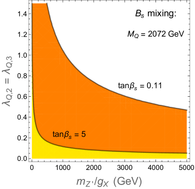
(a)

(b)

Figure 1: (a) The parameter space consistent with constraints from $B_{s}$ mixing in the ($m_{Z^{\prime}}/g_{Z}$, ${\lambda}_{Q,2}={\lambda}_{Q,3}$) plane for two choices of $\tan\beta_{S}$: $\tan\beta_{S}=0.11$ in orange and $\tan\beta_{S}=5$ in yellow. (b) The impact of the $R_{K}/R_{K^{\ast}}$ constraints on the $C_{9,\textrm{NP}}^{\mu}$ and $C_{10,\textrm{NP}}^{\mu}$ Wilson coefficients (Eqs. (14) and (15)) in the same plane, for the same two choices of $\tan\beta_{S}$.

In Fig. 1(a) we show in the ($m_{Z^{\prime}}/g_{X}$, ${\lambda}_{Q,2}={\lambda}_{Q,3}$) plane the parameter space consistent at the $2\,\sigma$ level with the $B_{s}$ mixing measurementDiLuzio:2017fdq . We choose two representative values of $\tan\beta_{S}$: $\tan\beta_{S}=0.11$ (orange parameter space) and $\tan\beta_{S}=5$ (yellow). Note that the parameter space is much more constrained for $\tan\beta_{S}>1$, due to the fact that the mixing between the U(1)_X-charged quark $D_{L}$ and the SM down-type quarks is directly proportional to the $v_{1}$ vev only. This is a feature that will affect the bounds on the quark mixing sector throughout this work.

In Fig. 1(b) we show the impact of the $R_{K}/R_{K^{\ast}}$ constraint on the $C_{9,\textrm{NP}}^{\mu}$ and $C_{10,\textrm{NP}}^{\mu}$ Wilson coefficients – i.e. Eqs. (14) and (15) are satisfied within the colored regions – in the ($m_{Z^{\prime}}/g_{X}$, ${\lambda}_{Q,2}={\lambda}_{Q,3}$) plane, for the same two choices of $\tan\beta_{S}$. Again, one can see that much larger parameter space is available when $\tan\beta_{S}\ll 1$.

3.2 Muon g – 2 and connections to dark matter

We recall that, once recent estimates of the hadronic and light-by-light scattering uncertainties are taken into account, the measured value of the anomalous magnetic moment of the muon, $(g-2)_{\mu}$, shows a $\sim 3.5\,\sigma$ discrepancy with the SM: $\delta\left(g-2\right)_{\mu}=(27.4\pm 7.6)\times 10^{-10}$Davier:2016iru . (Another recent review of the hadronic vacuum polarization contributions and uncertaintiesJegerlehner:2017lbd yields an even more convincing $\delta\left(g-2\right)_{\mu}=(31.3\pm 7.7)\times 10^{-10}$.) In our model one observes several contributions to the calculation of $(g-2)_{\mu}$ in addition to those of the MSSM. These extra terms can allow a good fit to the $(g-2)_{\mu}$ anomaly within a SUSY spectrum of broader mass range than in the MSSM.

At the one-loop level, the dominant new-physics contribution to $(g-2)_{\mu}$ can be roughly subdivided into two categoriesLeveille:1977rc ; Moore:1984eg . First, there are those due to neutral scalar fields (collectively indicated by $S^{0}$) and electrically charged fermions (collectively indicated by $E^{\pm}$), which read

$$\delta\left(g-2\right)_{\mu}=\frac{1}{16\pi^{2}}\sum_{S^{0},E^{\pm}}\left[\frac{m_{\mu}^{2}}{m_{S^{0}}^{2}}\left(|c_{L}|^{2}+|c_{R}|^{2}\right)\mathcal{F}_{1}(r)+2\,\frac{m_{\mu}m_{E^{\pm}}}{m_{S^{0}}^{2}}\,\Re(c_{L}c_{R}^{\ast})\,\mathcal{F}_{2}(r)\right]\,,$$ (28)

where $m_{\mu}$ is the muon mass, $c_{L}$ and $c_{R}$ are the direct couplings of the BSM fields to the left- and right-chiral states of the muon, respectively, $r\equiv(m_{E^{\pm}}/m_{S^{0}})^{2}$, and the loop functions are given by

$$\mathcal{F}_{1}(r) \equiv \frac{2+3r-6r^{2}+r^{3}+6r\ln r}{6\,(r-1)^{4}},$$ (29)

$$\mathcal{F}_{2}(r) \equiv \frac{3-4r+r^{2}+2\ln r}{2\,(r-1)^{3}}\,.$$ (30)

Secondly, there are those from charged scalars $S^{\pm}$ and neutral fermions $E^{0}$ in the loop:

$$\delta\left(g-2\right)_{\mu}=\frac{1}{16\pi^{2}}\sum_{S^{\pm},E^{0}}\left[-\frac{m_{\mu}^{2}}{m_{S^{\pm}}^{2}}\left(|c_{L}|^{2}+|c_{R}|^{2}\right)\mathcal{G}_{1}(r)+\frac{m_{\mu}m_{E^{0}}}{m_{S^{\pm}}^{2}}\,\Re(c_{L}c_{R}^{\ast})\,\mathcal{G}_{2}(r)\right]\,,$$ (31)

where

$$\mathcal{G}_{1}(r) \equiv \frac{1-6r+3r^{2}+2r^{3}-6r^{2}\ln r}{6(r-1)^{4}},$$ (32)

$$\mathcal{G}_{2}(r) \equiv \frac{-1+r^{2}-2r\ln r}{(r-1)^{3}}\,.$$ (33)

Note that Eq. (31) is negative when the fields of the new physics couple to just one of the chiral states of the muon, so that either $c_{L}$ or $c_{R}$ is equal zero, but it can become positive for $\Re(c_{L}c_{R}^{\ast})\neq 0$.

In addition to these two groups, one finds in our model contributions from the exchange of neutral vector fields (like the $Z^{\prime}$) and charged fermions in the loop, but they are subdominant in our model and we do not discuss them in what follows.

As is well known, in the presence of chirality-flip interactions of the new physics states with the muon (the term in $c_{L}c_{R}^{\ast}$ in Eqs. (28) and (31)) the calculation of $(g-2)_{\mu}$ receives a welcome boost from BSM contributions proportional to the bare mass of the new VL fermions, $m_{E}$Grifols:1982vx ; Czarnecki:2001pv ; Kowalska:2017iqv . However, it is also well known (see, e.g.,Fukushima:2014yia ) that these contributions introduce sizable, albeit cut-off independent, loop contributions in the calculation of the muon mass, as the latter is not in this case protected by chiral symmetry. One finds

$$\delta m_{\mu}\sim\frac{m_{E}}{16\pi^{2}}\Re\left(c_{L}c_{R}^{\ast}\right)\log\left(\frac{m_{E_{2}}}{m_{E_{1}}}\right)\sim\frac{m_{E}}{16\pi^{2}}\Re\left(c_{L}c_{R}^{\ast}\right)\log\left(\frac{m_{S_{2}}}{m_{S_{1}}}\right)\,$$ (34)

for any pair of mixing fermions $m_{E_{1,2}}$ (or scalars $m_{S_{1,2}}$) in the loop. This problem is generally dealt with by adjusting the value of the muon Yukawa coupling (which is not strongly constrained experimentally) until the large loop corrections are canceled point by point in the parameter space. We have designed our numerical scans so to have this procedure automatically carried out. The benchmark points we present in Sec. 4 are all characterized by the physical muon mass within $\sim 30\%$ of the experimental value, where we have left some room for the unknown uncertainties of higher-order loop contributions.

(a)

(b)

(c)

Figure 2: (a) The contribution to $(g-2)_{\mu}$ from the singlet scalars and VL lepton fields. (b), (c) Examples of contributions from neutralino/slepton loops that cannot be found in the MSSM. In all cases it is implied the photon line is attached to the electrically charged particle in the loop.

As pertains to the contributions to $(g-2)_{\mu}$, in the regular MSSMMoroi:1995yh ; Martin:2001st these are generated by chargino/sneutrino loops, corresponding to Eq. (28), and neutralino/smuon loops, corresponding to Eq. (31). In the model described here, though, there exist important extra terms.

A first class of these diagrams are induced by the neutral (pseudo)scalars $h^{\prime}$, $H^{\prime}$, $A^{\prime}$, and the charged heavy leptons corresponding to $L^{\prime}$ and $E^{\prime}$, as shown in Fig. 2(a). By parameterizing the mixing of the new scalar and pseudoscalar fields via the angles $\alpha^{\prime}$ and $\alpha^{\prime\prime}$, respectively, as is done in Appendix A, one can express the couplings of the new scalars to the left- and right-chiral components of the muon and the 5 physical charged leptons, labeled here in order of increasing mass, $I=1,..,5$:

$$c_{L}^{I\,h^{\prime}} = {\lambda}_{E,2}\cos\alpha^{\prime}D^{\prime{\dagger}}_{L\,25}D^{\prime{\dagger}}_{R\,I2}+{\lambda}_{L,2}\left(-\sin\alpha^{\prime}\right)D^{\prime{\dagger}}_{L\,22}D^{\prime{\dagger}}_{R\,I4}$$ (35)

$$c_{L}^{I\,H^{\prime}} = {\lambda}_{E,2}\sin\alpha^{\prime}D^{\prime{\dagger}}_{L\,25}D^{\prime{\dagger}}_{R\,I2}+{\lambda}_{L,2}\cos\alpha^{\prime}D^{\prime{\dagger}}_{L\,22}D^{\prime{\dagger}}_{R\,I4}$$ (36)

$$c_{L}^{I\,A^{\prime}} = i\left({\lambda}_{E,2}\sin\alpha^{\prime\prime}D^{\prime{\dagger}}_{L\,25}D^{\prime{\dagger}}_{R\,I2}+{\lambda}_{L,2}\cos\alpha^{\prime\prime}D^{\prime{\dagger}}_{L\,22}D^{\prime{\dagger}}_{R\,I4}\right),$$ (37)

$$c_{R}^{I\,h^{\prime}} = {\lambda}_{E,2}\cos\alpha^{\prime}D^{\prime{\dagger}}_{R\,22}D^{\prime{\dagger}}_{L\,I5}+{\lambda}_{L,2}\left(-\sin\alpha^{\prime}\right)D^{\prime{\dagger}}_{R\,24}D^{\prime{\dagger}}_{L\,I2}$$ (38)

$$c_{R}^{I\,H^{\prime}} = {\lambda}_{E,2}\sin\alpha^{\prime}D^{\prime{\dagger}}_{R\,22}D^{\prime{\dagger}}_{L\,I5}+{\lambda}_{L,2}\cos\alpha^{\prime}D^{\prime{\dagger}}_{R\,24}D^{\prime{\dagger}}_{L\,I2}$$ (39)

$$c_{R}^{I\,A^{\prime}} = i\left({\lambda}_{E,2}\sin\alpha^{\prime\prime}D^{\prime{\dagger}}_{R\,22}D^{\prime{\dagger}}_{L\,I5}+{\lambda}_{L,2}\cos\alpha^{\prime\prime}D^{\prime{\dagger}}_{R\,24}D^{\prime{\dagger}}_{L\,I2}\right),$$ (40)

where the fermion mixing matrices $D^{\prime\,{\dagger}}_{L,R}$ are defined as in Eq. (22). Our numerical analysis is based on a full one-loop numerical calculation, which takes into account all of the diagrams and couplings contributing to the measured observable. It is however worth briefly taking a look at a parametric approximation for the dominant contributions to $(g-2)_{\mu}$.

In the limit $\tan\beta\gg 1$, the contribution from one of the new scalar fields, say $H^{\prime}$, and VL leptons reads

$$\delta\left(g-2\right)_{\mu}^{(H^{\prime})}\sim\frac{m_{\mu}\widetilde{Y}_{2}v_{u}}{16\pi^{2}m_{H^{\prime}}^{2}}\,{\lambda}_{L,2}{\lambda}_{E,2}\,\sin 2\alpha^{\prime}\\ \times\left[\frac{m_{e_{5}}\max\left(M_{L},M_{E}\right)}{m_{e_{5}}^{2}-m_{e_{4}}^{2}}\mathcal{F}_{2}(r_{5})-\frac{m_{e_{4}}\min\left(M_{L},M_{E}\right)}{m_{e_{5}}^{2}-m_{e_{4}}^{2}}\mathcal{F}_{2}(r_{4})\right],$$ (41)

where $m_{e_{4}},m_{e_{5}}$ are the masses of the heaviest charged leptons in the spectra and $r_{i}=m_{e_{i}}^{2}/m_{H^{\prime}}^{2}$.

(a)

(b)

Figure 3: (a) The region of the ($M_{L}$, $M_{E}$) plane yielding $\delta\left(g-2\right)_{\mu}$ in agreement with the experimental measurement at $2\,\sigma$, if only the contribution of Eq. (41) is taken into account. In orange, ${\lambda}_{L,2}={\lambda}_{E,2}=0.4$ ; in yellow, ${\lambda}_{L,2}={\lambda}_{E,2}=0.8$ . The scalar mass and mixing parameters are fixed to typical values featured in the legend. (b) In the ($m_{\tilde{e}_{1}}$, $M_{\tilde{Z}^{\prime}}$) plane the parameter space in agreement with the measurement of $\delta\left(g-2\right)_{\mu}$ at the $2\,\sigma$ level, if only the contribution of Eq. (44) is considered. In yellow $g_{X}=0.4$ and in orange $g_{X}=0.8$. Other relevant parameters are fixed to the values given in the legend.

We plot in Fig. 3(a) the parameter space regions yielding $\delta\left(g-2\right)_{\mu}$ within $2\,\sigma$ of the measured value using only the contribution given by Eq. (41). The figure is presented in the plane of the bare superpotential VL lepton mass terms, ($M_{L}$, $M_{E}$), for two choices of new Yukawa couplings, ${\lambda}_{L,2}={\lambda}_{E,2}=0.4$ (orange region) and ${\lambda}_{L,2}={\lambda}_{E,2}=0.8$ (yellow region). A few other parameters of relevance are fixed as in the legend. One can see that the contribution from Eq. (41) becomes larger when the separation between the bare mass parameters is made large ($M_{L}\gg M_{E}$ or vice versa), and/or when lepton mixing due to the MSSM Higgs vev is sizable. The reader should be aware, on the other hand, that contributions to $\delta\left(g-2\right)_{\mu}$ from other (pseudo)scalars ($h^{\prime}$, $A^{\prime}$) tend to cancel the contributions of Eq. (41), as at least one of them always enters with opposite sign. In order to reduce the cancellation one is thus bound to consider parameter space characterized by $m_{H^{\prime}}\gg m_{h^{\prime}}$, and the mixing angles relative to $H^{\prime}$, $A^{\prime}$ should be preferably such that $\sin\alpha^{\prime\prime}\approx\sin\alpha^{\prime}$, $\cos\alpha^{\prime\prime}\approx\cos\alpha^{\prime}$.

It is important to note that contributions to $\delta\left(g-2\right)_{\mu}$ due to new scalar/VL lepton loops, like Eq. (41), do not depend on the parameters of the neutralino sector and can in principle be present independently of the specific features of the SUSY spectrum. A consequence of this is that in principle, by means of these contributions alone, the model is able to resolve the $(g-2)_{\mu}$ anomaly for much broader range of DM mass values and properties than in the MSSM.

There is, however, a second class of important diagrams that contribute to $(g-2)_{\mu}$. They involve combinations of the 7 neutralinos and 10 sleptons of the model, see for example Fig. 2(b) and Fig. 2(c). After ordering the neutralinos and sleptons by their increasing mass, $I=1,..,7$, $K=1,..,10$, one can write the full expression for the couplings to the muon chiral states,

$$c_{L}^{IK} = -\sqrt{2}g_{1}\left(y_{e_{L}}D^{\prime{\dagger}}_{L\,22}R^{n}_{I1}R^{s}_{K3}+y_{E_{L}}D^{\prime{\dagger}}_{L\,24}R^{n}_{I1}R^{s}_{K7}+y_{E^{\prime}}D^{\prime{\dagger}}_{L\,25}R^{n}_{I1}R^{s}_{K9}\right)$$ (42)

$$- \sqrt{2}g_{2}\left(T^{3}_{e_{L}}D^{\prime{\dagger}}_{L\,22}R^{n}_{I2}R^{s}_{K3}+T^{3}_{E_{L}}D^{\prime{\dagger}}_{L\,24}R^{n}_{I2}R^{s}_{K7}\right)-Y_{e,22}D^{\prime{\dagger}}_{L\,22}R^{n}_{I3}R^{s}_{K4}$$

$$- \widetilde{Y}_{1}D^{\prime{\dagger}}_{L\,24}R^{n}_{I3}R^{s}_{K10}-\widetilde{Y}_{2}D^{\prime{\dagger}}_{L\,25}R^{n}_{I4}R^{s}_{K8}$$

$$- \sqrt{2}g_{X}Q_{X}D^{\prime{\dagger}}_{L\,22}R^{n}_{I5}R^{s}_{K3}-{\lambda}_{L,2}D^{\prime{\dagger}}_{L\,22}R^{n}_{I6}R^{s}_{K8}+{\lambda}_{E,2}D^{\prime{\dagger}}_{L\,25}R^{n}_{I7}R^{s}_{K4}\,;$$

$$c_{R}^{IK} = -\sqrt{2}g_{1}\left(y_{e_{R}}D^{\prime{\dagger}}_{R\,22}R^{n}_{I1}R^{s}_{K4}+y_{E_{R}}D^{\prime{\dagger}}_{R\,24}R^{n}_{I1}R^{s}_{K8}+y_{E}D^{\prime{\dagger}}_{R\,25}R^{n}_{I1}R^{s}_{K\,10}\right)$$ (43)

$$- \sqrt{2}g_{2}T^{3}_{E_{R}}D^{\prime{\dagger}}_{R\,24}R^{n}_{I2}R^{s}_{K8}-Y_{e,22}D^{\prime{\dagger}}_{R\,22}R^{n}_{I3}R^{s}_{K3}$$

$$- \widetilde{Y}_{1}D^{\prime{\dagger}}_{R\,25}R^{n}_{I3}R^{s}_{K7}-\widetilde{Y}_{2}D^{\prime{\dagger}}_{R\,24}R^{n}_{I4}R^{s}_{K9}$$

$$- \sqrt{2}g_{X}Q_{X}D^{\prime{\dagger}}_{R\,22}R^{n}_{I5}R^{s}_{K4}-{\lambda}_{L,2}D^{\prime{\dagger}}_{R\,24}R^{n}_{I6}R^{s}_{K3}+{\lambda}_{E,2}D^{\prime{\dagger}}_{R\,22}R^{n}_{I7}R^{s}_{K9}\,,$$

in terms of the lepton, slepton, and neutralino mixing matrices defined as in Appendix A, gauge couplings $g_{1},g_{2},g_{X}$, isospin $T^{3}$, and hypercharge assignment $y$.

We point out that for this second class of important contributions we expect effects that largely extend the parameter space consistent with the measurement of $(g-2)_{\mu}$ with respect to the MSSM. Let us consider, for example, the well-known MSSM case of a nearly pure higgsino DM particle with a mass of $\sim 1\,\mathrm{TeV}$. In the MSSM neutralino/slepton loop contributions to $(g-2)_{\mu}$ for a $\sim 1\,\mathrm{TeV}$ higgsino typically involve the product of one of the gauge couplings $g_{1},g_{2}$ and the small muon Yukawa coupling, and are suppressed by the negligible $R_{12}^{n}(R_{13}^{n})^{{\dagger}}$ mixing. Conversely, Eqs. (42) and (43) show that in the U(1)-extended model one can rely on the product of sizable gauge and/or Yukawa couplings ($2g_{X}^{2}$, ${\lambda}_{L,2}{\lambda}_{E,2}$, etc.) and large mixing angles to boost the calculated value of $(g-2)_{\mu}$.

To guide the eye, we explicitly write down a parametric approximation of the contribution to $\delta\left(g-2\right)_{\mu}$ due to the $Z^{\prime}$-ino and the two lightest sleptons in the spectrum, cf. Fig. 2(b). One gets

$$\delta\left(g-2\right)_{\mu}^{(\tilde{Z^{\prime}})}\simeq\frac{g_{X}^{2}}{16\pi^{2}}m_{\mu}M_{\tilde{Z}^{\prime}}\sin 2\theta_{\textrm{eff}}\left[\frac{\mathcal{G}_{2}(t_{1})}{m_{\tilde{e}_{1}}^{2}}-\frac{\mathcal{G}_{2}(t_{2})}{m_{\tilde{e}_{2}}^{2}}\right],$$ (44)

in terms of an effective slepton mixing angle, $\theta_{\textrm{eff}}$, and where we define $t_{i}=M_{\tilde{Z}^{\prime}}^{2}/m_{\tilde{e}_{i}}^{2}$ as the squared ratio of the $Z^{\prime}$-ino mass to the $i$-th slepton mass. Typical values for $\sin 2\theta_{\textrm{eff}}$ range in the ballpark of $0.1-0.5$, and its parametric expansion strongly depends on the particular chosen point in the parameter space. When the lightest sleptons are nearly pure smuon gauge eigenstates one gets, for example, $\sin 2\theta_{\textrm{eff}}\approx 2\,Y_{e,22}\,v_{u}(\mu\tan\beta-A_{\mu})/(m_{\tilde{e}_{2}}^{2}-m_{\tilde{e}_{1}}^{2})$ .

We show in Fig. 3(b) the parameter space in the ($m_{\tilde{e}_{1}}$, $M_{\tilde{Z}^{\prime}}$) plane in agreement with the measured $\delta\left(g-2\right)_{\mu}$ at the $2\sigma$ level, and with a $\sim 1\,\mathrm{TeV}$ higgsino DM candidate. We plot exclusively the contribution due to Eq. (44), with $\sin 2\theta_{\textrm{eff}}=0.3$. The region in yellow is obtained when $g_{X}=0.4$, the region in orange when $g_{X}=0.8$, and the other relevant parameters are fixed to the values given in the legend. One can then see that the parameter space is much extended with respect to the MSSMKowalska:2015zja .

To conclude this section, we point out that in the most realistic cases the contribution to $(g-2)_{\mu}$ is given by a combination of all of these effects, which can sum and subtract from each other in a complicated way, depending on the parameter space region at hand. In particular, in the benchmark points we present is Sec. 4, $\delta\left(g-2\right)_{\mu}$ is obtained in agreement with the measured value always as a result of the combination of many different diagrams, without one single mechanism playing a dominant role.

4 Numerical results and benchmark scenarios

In this section we present benchmark scenarios that fit the flavor constraints discussed in Sec. 3 and are representative of different interesting parameter space regions of the model. We also analyze their DM properties and give an overview of the typical LHC bounds.

4.1 Benchmark points

Each benchmark point was generated with the numerical package SARAH v.4.12.2Staub:2013tta . 1-loop corrected mass spectra and decay branching ratios were calculated with the corresponding SPhenoPorod:2003um ; Porod:2011nf modules, automatically produced by SARAH. Low-energy observables, including $\delta\left(g-2\right)_{\mu}$, have been calculated with SPheno, while to derive the Wilson coefficients $C_{9,\textrm{NP}}^{\mu}$ and $C_{10,\textrm{NP}}^{\mu}$, as well as the parameter $R_{BB}$, we used analytic tree-level formulas (3.1) and (19). Dark matter related observables were calculated with MicrOMEGAs v.4.3.1Belanger:2013oya , based on the CalcHEPBelyaev:2012qa files generated by SARAH. To efficiently scan the multidimensional space of input model parameters, we interfaced all the employed numerical packages to MultiNest v.3.10Feroz:2008xx driven by a global likelihood function.

Parameter BP1 BP2 BP3 BP4 BP5 BP6 BP7 BP8 ${m_{0}}$ $2678$ $2957$ $1915$ $1548$ $3017$ $2278$ $2481$ $2291$ $m_{\tilde{q},33}\!=\!m_{\tilde{u},33}$ $7156$ $5007$ $4956$ $4062$ $5489$ $5236$ $6068$ $5390$ $M_{1,2}$ $3920$ $2726$ $1913$ $2463$ $1906$ $1839$ $2924$ $2128$ $M_{3}$ $2615$ $3167$ $2911$ $3148$ $2990$ $3024$ $2849$ $3106$ $A_{0}$ $-\,5625$ $-\,2588$ $-\,4286$ $-\,4208$ $-\,5468$ $-\,4355$ $-\,2117$ $-\,5327$ $B_{0}$ $-\,918$ $-\,1486$ $-\,1456$ $-\,1159$ $-\,756$ $-\,745$ $-\,1623$ $-\,1344$ $\mu$ $1013$ $1143$ $1509$ $1128$ $1265$ $1725$ $1044$ $1098$ $B_{\mu}\,[10^{5}]$ $4.8$ $1.9$ $5.1$ $3.5$ $4.7$ $2.8$ $1.4$ $3.2$ $\tan\beta$ $47.9$ $53.3$ $48.9$ $47.0$ $42.3$ $36.6$ $35.3$ $43.0$ $M_{Q}$ $1900$ $2000$ $2672$ $2182$ $2000$ $2110$ $1800$ $1888$ $M_{L}$ $2230$ $954$ $915$ $2450$ $2972$ $1364$ $815$ $1174$ $M_{E}$ $701$ $700$ $1046$ $2141$ $497$ $1534$ $2262$ $801$ ${\lambda}_{Q,2}={\lambda}_{Q,3}$ $0.08$ $0.07$ $0.80$ $0.15$ $0.08$ $0.80$ $1.10$ $0.07$ ${\lambda}_{L,2}$ $-\,1.2$ $-0.895$ $-\,0.579$ $-\,0.404$ $-\,1.069$ $-\,1.380$ $-\,1.05$ $0.436$ ${\lambda}_{E,2}$ $-\,0.8$ $0.908$ $-\,0.746$ $-\,0.921$ $-\,0.520$ $0.705$ $-\,0.713$ $-\,1.452$ $\widetilde{Y}_{1}$ $0.855$ $-0.426$ $0.098$ $0.450$ $-\,0.338$ $-\,0.567$ $-\,0.615$ $-\,1.144$ $\widetilde{Y}_{2}$ $0.525$ $0.651$ $0.245$ $-\,0.903$ $-\,0.699$ $0.388$ $-\,0.958$ $-\,0.435$ $\mu_{S}$ $-\,1270$ $-\,2161$ $-\,388$ $968$ $1125$ $-\,1764$ $-\,399$ $-\,994$ $B_{\mu_{S}}\,[10^{6}]$ $-\,3.5$ $-\,0.9$ $-\,1.2$ $-\,3.9$ $-\,4.7$ $-\,3.4$ $-\,1.3$ $-\,1.0$ $\tan\beta_{S}$ $13.6$ $4.9$ $0.11$ $0.73$ $6.4$ $0.11$ $0.06$ $12.7$ $m_{Z^{\prime}}$ $500$ $351$ $310$ $472$ $419$ $798$ $430$ $690$ $M_{\tilde{Z}^{\prime}}$ $1943$ $1592$ $1151$ $1385$ $1844$ $641$ $815$ $491$ $g_{X}$ $0.79$ $0.376$ $0.53$ $0.66$ $0.62$ $0.87$ $0.63$ $0.76$ $Y_{e,22}$ $0.016$ $-\,0.087$ $0.029$ $0.026$ $0.034$ $-\,0.015$ $-\,0.018$ $-\,0.012$

Table 1: Input parameters at the SUSY scale for our benchmark scenarios. Dimensionful quantities are given in GeV and $\,\mathrm{GeV}^{2}$.

We show in Tables 1 and 2 eight chosen benchmarks scenarios. In Table 1 we present their input parameter values. The top panel of the table gives typical values for the relevant MSSM input parameters; the bottom panel holds instead the values associated with the U(1)_X sector.

BP1 BP2 BP3 BP4 BP5 BP6 BP7 BP8 $m_{\chi^{0}_{1}}$ $1042$ $1165$ $328$ $848$ $1071$ $429$ $257$ $273$ $m_{\tilde{{\chi}}^{0}_{2}}$ $1044$ $1168$ $417$ $1046$ $1186$ $1719$ $470$ $1118$ $m_{{\chi}^{\pm}_{1}}$ $1043$ $1167$ $1529$ $1153$ $1289$ $1731$ $1068$ $1120$ $m_{\tilde{g}}$ $2867$ $3373$ $3029$ $3176$ $3238$ $3171$ $3034$ $3226$ $m_{h}$ $125.5$ $123.6$ $123.2$ $125.6$ $126.0$ $123.6$ $125.1$ $124.6$ $m_{A,H}$ $3830$ $2128$ $4189$ $3108$ $3752$ $1996$ $1753$ $2765$ $m_{h^{\prime}}$ $487$ $360$ $291$ $423$ $402$ $739$ $406$ $645$ $m_{A^{\prime},H^{\prime}}$ $6788$ $2475$ $3026$ $5031$ $5558$ $5083$ $4309$ $3508$ $m_{e_{4}}$ $706$ $706$ $937$ $2109$ $503$ $1386$ $830$ $797$ $m_{e_{5}}$ $2301$ $1139$ $1094$ $2490$ $3026$ $1602$ $2256$ $1226$ $M_{\rm SUSY}$ $3117$ $3446$ $2785$ $2334$ $3417$ $2863$ $3030$ $2837$ $m_{\tilde{e}_{1}}$ $2521$ $2693$ $1596$ $1524$ $2928$ $2096$ $2444$ $2031$ $m_{\tilde{e}_{2}}$ $2656$ $2780$ $1811$ $1555$ $2988$ $2223$ $2478$ $2089$ $m_{Z^{\prime}}$ $491$ $348$ $303$ $465$ $412$ $791$ $423$ $684$ $m_{u_{4}}\!\approx\!m_{d_{4}}$ $2164$ $2227$ $2436$ $2433$ $2246$ $2379$ $2035$ $2140$ $\Omega_{\chi}h^{2}$ $0.11$ $0.12$ $0.10$ $0.11$ $0.11$ $0.10$ $0.11$ $0.10$ $N_{\textrm{higgsino}}$ $99.9\%$ $99.8\%$ $0$ $0$ $0$ $0$ $0$ $0$ $N_{\tilde{S}_{1}}$ $0$ $0$ $53\%$ $32\%$ $41\%$ $18\%$ $57\%$ $33\%$ $N_{\tilde{S}_{2}}$ $0$ $0$ $40\%$ $48\%$ $50\%$ $2\%$ $25\%$ $4\%$ $N_{\tilde{Z}^{\prime}}$ $0$ $0$ $7\%$ $20\%$ $9\%$ $80\%$ $18\%$ $63\%$ $\sigma^{\rm SI}_{p}\times 10^{46}$ $0.63$ $2.4$ $1\!\times\!10^{-3}$ $8\!\times\!10^{-3}$ $4\!\times\!10^{-2}$ $4\!\times\!10^{-4}$ $1\!\times\!10^{-2}$ $2\!\times\!10^{-3}$ $\sigma v\times 10^{26}$ $0.9$ $1.0$ $1.3$ $2.2$ $2.1$ $7\!\times\!10^{-3}$ $3\!\times\!10^{-4}$ $4\!\times\!10^{-5}$ final state $WW/ZZ$ $WW/ZZ$ $Z^{\prime}/h^{\prime}\,Z^{\prime}$ $Z^{\prime}/h^{\prime}\,Z^{\prime}$ $Z^{\prime}/h^{\prime}\,Z^{\prime}$ $\bar{e}_{3}\,e_{3}$ $\bar{u}_{3}\,u_{3}$ $\bar{u}_{3}\,u_{3}$ $\delta\left(g-2\right)_{\mu}\!\times\!10^{9}$ $2.1$ $1.6$ $1.6$ $1.3$ $1.4$ $1.1$ $1.3$ $2.3$ $C^{\mu}_{9,\textrm{NP}}$ $-\,1.04$ $-\,0.61$ $-\,0.67$ $-\,0.99$ $-\,0.93$ $-\,1.02$ $-\,0.71$ $-\,0.81$ $C^{\mu}_{10,\textrm{NP}}$ $-\,0.03$ $-\,0.08$ $0.02$ $0.01$ $-\,0.01$ $0.04$ $0.01$ $-\,0.02$ $R_{BB}\times 10^{3}$ $2$ $2$ $0.6$ $2$ $2$ $4$ $0.9$ $2$ $\textrm{BR}_{h\to\mu\mu}\times 10^{4}$ $2.0$ $4.8$ $3.5$ $3.1$ $4.1$ $<10^{-4}$ $3.2$ $<10^{-4}$ $Z^{\prime}$ decays $\bar{e},\bar{\nu}_{2,3}\,e,\nu_{2,3}$ $h^{\prime}$ decays $ZZ$, $WW$ $\chi^{0}_{1}\chi^{0}_{1}$ $ZZ,\!WW$ $\chi^{0}_{1}\chi^{0}_{1}$ $e_{4}$ decays $e_{2}\,h^{\prime}$, $e_{2}\,Z^{\prime}$

Table 2: Spectrum and various observables for our benchmark points. Masses are given in GeV, spin-independent cross section $\sigma^{\rm SI}_{p}$ in cm², and present-day annihilation cross section $\sigma v$ in cm³/s. We define, as usual, $M_{\rm SUSY}=(m_{\tilde{t}_{1}}m_{\tilde{t}_{2}})^{1/2}$ as the geometrical average of stop masses.

In Table 2 we present physical masses and some mixing parameters of the selected benchmark points, and give the value of the observables of interest. All the benchmark points featured in the tables are characterized by $\delta\left(g-2\right)_{\mu}$ in agreement with the experimental determination within $2\,\sigma$, the loop-corrected muon mass within 30% of the measured value, and $C_{9,\textrm{NP}}^{\mu}$ and $C_{10,\textrm{NP}}^{\mu}$ in agreement with the estimates of the most recent global fits, Eqs. (14) and (15).

4.2 Dark matter

Depending on the properties of the lightest SUSY particle (LSP), our neutralino DM can be divided into three different categories. Note, however, that we focus here on the states typical of our $Z^{\prime}$-extended model and refrain from addressing those solutions giving the relic density and $(g-2)_{\mu}$ in the MSSM, which generally involve a bino-like neutralino LSP co-annihilating in the early Universe with a slepton, or undergoing $s$-channel resonant annihilation mediated by one of the MSSM Higgs fields. (Note that slepton-coannihilation and $A/H$-funnel are also the favorite DM mechanisms in minimal MSSM extensions by a pair of VL fermion multiplets of the SU(5) group, which also contribute positively to the $(g-2)_{\mu}$ calculationChoudhury:2017fuu .)

$\bullet$ BP1-BP2: 1 TeV higgsino and the XENON-1T excess. Benchmarks BP1 and BP2 feature a $\sim 1\,\mathrm{TeV}$ higgsino LSP ($\mu\approx 1\,\mathrm{TeV}\approx m_{\chi_{1}^{0}}\approx m_{\chi_{1}^{\pm}}\approx m_{\chi_{2}^{0}}$), which is a well studied DM particle of the MSSMProfumo:2004at . Unlike in the MSSM, however, where typically there does not exist a solution for the $(g-2)_{\mu}$ anomaly in the parameter space with a $\sim 1\,\mathrm{TeV}$ higgsino, due to the associated large mass for the sleptons in the spectrum, in this model $\delta\left(g-2\right)_{\mu}^{\textrm{BP1,BP2}}>10^{-9}$.

The enhanced $(g-2)_{\mu}$ value is due to a combination of the mechanisms described in Sec. 3.2. In the particular case of BP1, the largest contribution is given by new neutralino/slepton loops, which boost the value of the anomalous magnetic moment even in the presence of a fairly large slepton mass, thanks to the presence of several neutralino states not far above the $\sim 1\,\mathrm{TeV}$ scale, as illustrated in Fig. 3(b). In the case of BP2 the presence of a fairly light, $\lesssim 500\,\mathrm{GeV}$ scalar, $h^{\prime}$, associated with the breaking of the U(1)_X symmetry, introduces a sizable contribution to the scalar/VL lepton loop, as described in Sec. 3.2 and illustrated in Fig. 3(a). Note that in general, these new contributions require sizable, but not abnormally large, new Yukawa couplings: $|{\lambda}_{L,2}|,\,|{\lambda}_{E,2}|\mathrel{\hbox to0.0pt{\lower 4.0pt\hbox{\hskip 1.0pt$\sim$}\hss}\raise 1.0pt\hbox{$>$}}0.5$.

Interestingly, benchmark points like BP1 and BP2 feature a typical value of the spin-independent cross section, $\sigma^{\rm SI}_{p}$, large enough to provide a possible explanation for the slight excess of events observed in the XENON-1T 1-year dataAprile:2018dbl . The XENON Collaboration has recorded a few events over the background consistent at $\sim 1\sigma$ with a best-fit point featuring $\sigma^{\rm SI}_{p}=4.7\times 10^{-47}\,\textrm{cm}^{2}$ for a WIMP mass $m_{\chi}=200\,\mathrm{GeV}$, or $\sigma^{\rm SI}_{p}\approx 1\!-\!2\times 10^{-46}\,\textrm{cm}^{2}$ for $m_{\chi}\approx 1\,\mathrm{TeV}$. A spin independent cross section of this size corresponds to a typical gaugino mass of about $2.5-3\,\mathrm{TeV}$. For recent reviews of the typical direct and indirect DM detection signatures of the $\sim 1\,\mathrm{TeV}$ higgsino in the MSSM, seeRoszkowski:2017nbc ; Kowalska:2018toh .

$\bullet$ BP3-BP5: Well-tempered $\boldsymbol{Z^{\prime}}$-ino/singlino. The three benchmark points BP3-BP5 represent scenarios in which the neutralino LSP is predominantly singlino, with a non-negligible admixture of $Z^{\prime}$-ino. The relic density is obtained thanks to a combination of different annihilation diagrams and final states, the most dominant of which is a $t$-channel exchange of the second singlino to pair-produce the lighter $Z^{\prime}$ or $h^{\prime}$ boson, as depicted in Fig. 4. This scenario is reminiscent of the “well-tempered” neutralino of the MSSMArkaniHamed:2006mb but, unlike the latter, it involves exclusively the neutralinos of the $Z^{\prime}$-related sector.

Figure 4: Example of early-Universe annihilation diagrams for highly-mixed $Z^{\prime}$-ino/singlino neutralinos, yielding to final states dominated by the $h^{\prime}$ and $Z^{\prime}$ bosons.

The parameter space spans over a wide range of neutralino mass values, which can be as heavy as $\sim 1\,\mathrm{TeV}$, and of spin-independent cross sections, typically in the range $\sigma^{\rm SI}_{p}=10^{-50}\!-\!10^{-46}\,\textrm{cm}^{2}$. Since the dominant interaction of the neutralino with nuclei in underground detectors stems in this case from a $t$-channel exchange of the scalar $h^{\prime}$, its strength is highly dependent on the size of the effective loop couplings that, on the one hand, connect $h^{\prime}$ to the gluons in the proton, and on the other, generate the mixing of $h^{\prime}$ with the SM Higgs (recall that at the tree level the scalar mass matrix is block-diagonal). Since to efficiently control the relative size of these effects one would need a detailed analysis of the loop interactions of the model, we do not attempt in this work to connect this type of mixed neutralino scenarios to the XENON-1T excess.

As pertains to the $(g-2)_{\mu}$ anomaly, the dominant contribution for BP3-BP5 is given by the neutralino/slepton loops, enhanced by the presence of several neutralinos not far above the $\sim 1\,\mathrm{TeV}$ scale, and sizable Yukawa couplings $|{\lambda}_{L,2}|,\,|{\lambda}_{E,2}|\mathrel{\hbox to0.0pt{\lower 4.0pt\hbox{\hskip 1.0pt$\sim$}\hss}\raise 1.0pt\hbox{$>$}}0.5$.

$\bullet$ BP6-BP8: $Z^{\prime}$ resonance.

The last set of benchmark points give examples of neutralinos that show a sizable $Z^{\prime}$-ino composition, with subdominant or equivalent singlino components. In the early Universe an annihilation cross section of the right size for the relic abundance can be obtained through an $s$-channel resonance with the fairly broad $Z^{\prime}$ boson, yielding to final states highly dominated by muons and taus, as is typical of $L_{\mu}-L_{\tau}$ models (see, e.g.,Sierra:2015fma ; Baek:2017sew ). We show the diagram for this process in Fig. 5.

As before, the spin-independent scattering cross section with protons is due to the exchange of a $h^{\prime}$ boson, and is consequently suppressed by loop effects. At the same time, the present-day annihilation cross-section, $\sigma v$, is suppressed by $p$-wave and thermal broadening, so that this scenario is difficult to detect by direct and indirect searches for DM. As we shall see in Sec. 4.3, since BP6-BP8 are characterized by a fairly light $Z^{\prime}$ boson, in the cases where $\tan\beta_{S}>1$ the best prospects for detection might be provided by the high-luminosity LHC (HL-LHC).

Figure 5: The dominant early-Universe annihilation channel for a predominantly $Z^{\prime}$-ino LSP.

Figure 6: The position of the benchmark points in the ($m_{\chi}$, $\sigma^{\rm SI}_{p}$) plane, compared to the current 90% C.L. upper bound from the XENON-1T CollaborationAprile:2018dbl . Different point-styles mark the different types of neutralinos described in Sec. 4.2.

We summarize in Fig. 6 the position of our eight benchmark points in the ($m_{\chi}$, $\sigma^{\rm SI}_{p}$) plane. The different types of neutralinos described above are marked with different style, according to the legend.

4.3 Additional constraints on the flavor structure

As we have seen in the previous sections, a proper fit to the $(g-2)_{\mu}$ and flavor anomalies requires the presence of an extra flavor structure beyond the MSSM. While flavor physics (and in particular $B_{s}$-mixing) provides the dominant constraint on our model, other BSM searches can also be relevant in certain regions of the parameter space.

Neutrino trident production

Since the $L_{\mu}-L_{\tau}$ gauge boson couples at the tree-level to muon and tau neutrinos, one can expect a strong enhancement in the neutrino trident production from scattering on atomic nuclei $N$: $N\nu\rightarrow\nu N\mu^{+}\mu^{-}$Altmannshofer:2014pba . The cross section for this process has been measured by the CCFRMishra:1991bv and CHARM-IIGeiregat:1990gz collaborations to be in agreement with the SM prediction, leading in the large $m_{Z^{\prime}}$ limit ($m_{Z^{\prime}}\mathrel{\hbox to0.0pt{\lower 4.0pt\hbox{\hskip 1.0pt$\sim$}\hss}\raise 1.0pt\hbox{$>$}}10\,\mathrm{GeV}$) to a generic bound:

$$m_{Z^{\prime}}/g_{X}\gtrsim 540\text{ GeV}\ .$$ (45)

This constraint typically provides a lower bound on the accessible $m_{Z^{\prime}}$ mass, independent of the remaining parameters of the flavor sector.

LHC Higgs measurements in the muon channel

We have mentioned in Sec. 3.2 that, since the largest contributions to the calculation of $(g-2)_{\mu}$ involve loop diagrams that violate chiral symmetry, one must proceed to tune the Yukawa coupling of the muon against large loop corrections to the muon mass. Thus, a powerful constraint on the benchmark points can be derived from measurement of SM Higgs decay in the $\mu\mu$ channel, which test directly the effective muon Yukawa coupling. The current experimental signal strength for this channel is $\sigma/\sigma^{SM}=0\pm 1.3$Tanabashi:2018 .

Since the mixing between the new Higgs sector and the MSSM one is loop-suppressed, the production mechanism for the 125$\,\mathrm{GeV}$ Higgs boson is to a good approximation similar to the one of the SM. Hence the quantity that determines directly the signal strength is the branching ratio to muons, which in the SM reads $\textrm{BR}(h_{\textrm{SM}}\rightarrow\mu\mu)=2.2\times 10^{-4}$Tanabashi:2018 . We report the corresponding value of the branching ratio for our benchmark points at the bottom of Table 2. Note that in all benchmark points we are within the current upper bound $\textrm{BR}(h_{\textrm{SM}}\rightarrow\mu\mu)<5.7\times 10^{-4}$, even if all points are characterized by significant loop contributions to $(g-2)_{\mu}$.

At the tree level, the branching ratio is directly proportional to the effective Yukawa coupling squared, $|Y_{\textrm{eff},22}|^{2}$, between the SM Higgs, $h_{\textrm{SM}}$, and the muon: $\mathcal{L}\supset-Y_{\textrm{eff},22}\,(h_{\textrm{SM}}\,e_{L,2}\,e_{R,2}$ $+$ $\textrm{h.c.})$. In our model, this effective coupling can be readily expressed as

$$Y_{\textrm{eff},22} = Y_{e,22}\left(-\sin\alpha\right)D^{\prime{\dagger}}_{L,22}D^{\prime{\dagger}}_{R,22}+\widetilde{Y}_{1}\left(-\sin\alpha\right)D^{\prime{\dagger}}_{L,24}D^{\prime{\dagger}}_{R,25}+\widetilde{Y}_{2}\left(\cos\alpha\right)D^{\prime{\dagger}}_{L,25}D^{\prime{\dagger}}_{R,24}\,,$$

where we use the rotation matrix elements defined in Eq. (22), and the Higgs rotation angle $\alpha$ is defined in Appendix A. In the large $\tan\beta$ limit, we find

$$|Y_{\textrm{eff},22}|^{2}\leavevmode\nobreak\ \approx\leavevmode\nobreak\ \frac{1}{\tan^{2}\beta}\frac{1}{\left(1+\frac{{\lambda}_{E,2}^{2}v_{2}^{2}}{2M_{E}^{2}}\right)\left(1+\frac{{\lambda}_{L,2}^{2}v_{1}^{2}}{2M_{L}^{2}}\right)}\left(Y_{e,22}+\widetilde{Y}_{1}\frac{v_{1}v_{2}\lambda_{E,2}\lambda_{L,2}}{2M_{E}M_{L}}\right)^{2}.$$ (46)

In particular, the effective Yukawa coupling contains a term originating from the new VL sector. Hence, depending on the values of $Y_{e,22}$ and $\widetilde{Y}_{1}$ the two terms can cancel out, leading to a branching ratio significantly lower than the SM value. This typically occurs in our benchmark points BP6 and BP8.

The main consequence of these effects is that, by increasing the sensitivity of Higgs searches in the muon channels, the LHC collaborations can constrain the Yukawa couplings of our models, which in turn will refine the predictions of our model for $(g-2)_{\mu}$ and flavor observables in general.

LHC exotica searches

The MSSM sector of the model could be in principle tested by a wide set of LHC SUSY searches. However, since all the anomalies discussed in Sec. 3 can be accommodated by setting the masses of the MSSM gluinos, charginos, squarks, and sleptons above the corresponding experimental lower bounds, we do not consider the impact of these searches in this work.

On top of the MSSM particles, the model presented in this paper can feature several new fields in the sub-TeV regime, including the new gauge boson an additional neutral Higgs boson, and the fourth and fifth-generation VL leptons. In the following, we will study the bounds on these states from existing LHC searches, to ensure that the benchmark points presented in Tables 1 and 2 are compatible with the experimental data. In our numerical analysis we use the UFO model file generated by SARAH v.4.12.2Staub:2013tta and passed to MadGraph5_aMC@NLOAlwall:2014hca to estimate the relevant LO cross sections times the branching ratio quantities.

$\boldsymbol{Z^{\prime}}$ signatures

The new gauge boson $Z^{\prime}$  couples to the SM fields either through its mixing with the $Z$ boson (which we assume to be negligible in this study), or through the mixing between the U(1)_X-charged VL quarks and their SM counterparts.

(a)

(b)

Figure 7: The dominant production and decay channels for the beyond the MSSM bosons. (a) Heavy quark fusion production of $Z^{\prime}$. (b) Gluon fusion production of $h^{\prime}$.

The dominant production mechanism of $Z^{\prime}$ is heavy quark fusion, as shown in Fig. 7(a). Since it can only proceed through the mixing of $Q$ with the $s$ and $b$ quarks, it is PDF-suppressed and crucially depends on the value of $v_{1}$, see Eq. (26). This implies that $Z^{\prime}$ production is strongly suppressed when $\tan\beta_{S}\ll 1$.

(a)

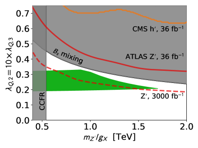
(b)

Figure 8: Bounds from $B_{s}$-mixing (gray area is excluded) and neutrino trident production (dark gray area is excluded). Upper exclusion bound from current ATLASAaboud:2017buh dilepton search (red line), our HL-LHC projection for the same analysis (dashed red line), di-$Z$ search from $h^{\prime}$ decay (orange line) and the region favored by the $R_{K^{(\ast)}}$ anomalies (green area), in the $\lambda_{Q,2}$ and $m_{Z^{\prime}}/g_{X}$ plane for the ratios (a) $\lambda_{Q,2}=\lambda_{Q,3}$, (b) and $\lambda_{Q,2}=10\times\lambda_{Q,3}$. All other parameters are chosen according to benchmark point BP1 (blue star) as presented in Tables 1 and 2 .

The dominant visible decay channel of $Z^{\prime}$ is into a pair of muons or taus. The strongest experimental limits at $\sqrt{s}=13\,\mathrm{TeV}$ are provided by the ATLASAaboud:2017buh and CMSSirunyan:2018exx high-mass resonance searches based on the dilepton channels for 36$\,\textrm{fb}^{-1}$ luminosity. The limits apply to the product of production cross section times the branching fraction into a pair of muons, as a function of the $Z^{\prime}$ mass. In Fig. 8(a) we show in red solid the 95% C.L. dilepton exclusion upper bound based on the ATLAS analysis as a function of the new Yukawa coupling $\lambda_{Q,2}$ and of the $Z^{\prime}$ mass, for the choice of other model parameters corresponding to BP1 (depicted with a blue triangle). We also present, as a red dashed line, our estimate of the potential reach of the HL-LHC with an integrated luminosity of 3000$\,\textrm{fb}^{-1}$.

Incidentally, note that the parameters of interest for the $Z^{\prime}$ production are $M_{Q}$, $\lambda_{Q,2}$, $v_{1}$ and $g_{X}$, the same that also enter the $B_{s}$ mixing. However, in contrast to the upper bounds from $B_{s}$-mixing (depicted in Fig. 8(a) as a gray shaded region), the $Z^{\prime}$ production relies mostly on the mixing between the VL quark $Q$ and the strange quark, and hence on the product $v_{1}\lambda_{Q,2}$. This implies that when the Yukawa couplings of the VL quarks present an inverted hierarchy, $\lambda_{Q,3}\ll\lambda_{Q,2}$, the exclusion bound bites more deeply into the region of the parameter space favored by the LFUV anomalies, shown here in green. We illustrate this effect in Fig. 8(b), in which we assume that $\lambda_{Q,2}=10\,\lambda_{Q,3}$. This feature opens up the possibility of experimentally testing the structure of the BSM flavor sector with the HL-LHC. Finally, the fact that the $Z^{\prime}$ is dominantly produced through its coupling to strange quarks sets apart the low-energy limit of our model from the effective approach ofKohda:2018xbc where it was found that a discovery at HL-LHC required large $B_{s}$-mixing values.

We do not show the corresponding exclusion bounds for other benchmark points from Table 1. As long as $\tan\beta_{S}\gg 1$ (BP2, BP5, and BP7), their dependence on the parameters of interest is exactly the same as the one shown in Fig. 8(a). If, on the other hand, $\tan\beta_{S}\ll 1$ (as is the case of BP3, BP4, BP6, and BP7), $Z^{\prime}$ production is strongly suppressed at the LHC and the dilepton searches do not provide any constraints for perturbative values of $\lambda_{Q,2}$.

New light Higgs decays

In order to open up an efficient mechanism for pair annihilation of the neutralino LSP in the early Universe, for BP3-BP5 the lightest of the two new neutral Higgs bosons, $h^{\prime}$, has a mass in the sub-TeV regime. Similarly the sub-TeV $Z^{\prime}$ and $h^{\prime}$ are favored by $(g-2)_{\mu}$ in the case of BP1 and BP2 and by the $Z^{\prime}$ resonance for BP6-BP8. When kinetic mixing is negligible, $h^{\prime}$ interacts with the SM particles either through its (loop-induced) mixing with the SM Higgs, or through the loops mediated by the new VL fermions. The dominant production channel of $h^{\prime}$ is gluon fusion, shown in Fig. 7(b), with an effective coupling to gluons $C_{h^{\prime}gg}$ generated via the two above-mentioned mechanisms. The former typically dominates for lighter $h^{\prime}$, while the latter for heavier.

Decays of the new Higgs boson are driven mostly by its mixing with the SM Higgs, with the highest branching ratios into $h^{\prime}\to W^{+}W^{-}$ and $h^{\prime}\to ZZ$ for the benchmark points shown in Table 1. Such decay channels have been studied by both the ATLAS and CMS collaborations, with the most recent results reported inAaboud:2017gsl ; Aaboud:2017fgj ; Aaboud:2017itg for the former, andSirunyan:2018qlb for the latter. While these searches can typically probe $\sigma\times\textrm{BR}$ values down to $10-100$ fb, in our model $h^{\prime}$ production is typically very suppressed by being loop-induced. Overall, we find that the corresponding experimental bounds, illustrated in Fig. 8LABEL:sub@fig:a as an orange solid line, are weaker than the ones from the $Z^{\prime}$ searches.

More generally, we observe that also in this case $\tan\beta_{S}$ is the key parameter that allows to access the new sector experimentally. Since only the $S_{1}$ scalar couples directly to the new heavy VL quarks, see Eq. (8), for $\tan\beta_{S}\ll 1$ the new light Higgs boson is effectively secluded from the SM.

Masses of VL fermions

The new VL leptons can be pair-produced at the LHC via Drell-Yan. Their preferential decay modes are $e_{4,5}\rightarrow e_{2}\,Z^{\prime}$, $e_{4,5}\rightarrow e_{2}\,h^{\prime}$ for lighter $Z^{\prime}$, and $e_{4,5}\rightarrow e_{2}\,Z$, $e_{4,5}\rightarrow e_{2}\,h$ when the $Z^{\prime}$ is heavier than all of the leptons. Multi-lepton searches at the LHC typically set constraints on these second type of decay chains, which translate into a lower bound on the VL lepton mass of the order of $M_{L},M_{E}\mathrel{\hbox to0.0pt{\lower 4.0pt\hbox{\hskip 1.0pt$\sim$}\hss}\raise 1.0pt\hbox{$>$}}200-300\,\mathrm{GeV}$, depending on the branching ratioDermisek:2014qca ; Kumar:2015tna .

In the bulk of our parameter space, however, the 4th and 5th lepton generations are generically heavier and decay preferentially via $Z^{\prime}$ and $h^{\prime}$. While the former lead to final states similar to the standard $Z$-induced decay (but with different kinematics due to the heavy mass of the $Z^{\prime}$), the latter typically implies final states with larger lepton and/or jets multiplicities, as $h^{\prime}$ decays in turn into a pair of $W$ or $Z$ bosons. No existing LHC bounds actually apply to these states, and deriving a constraint would require a full recasting, which exceeds the purposes of this work. Let us simply note that the pair production cross section for such states is typically very small: $\sigma_{pp\rightarrow L^{\prime}L^{\prime}}\approx 2\,\mathrm{fb}$ for VL lepton masses of around $500\,\mathrm{GeV}$.

It is easier to pair-produce the new VL quarks. Searches for heavy tops/bottoms have been regularly updated by both the ATLAS and CMS collaborations, with exclusion bounds implying $M_{Q}\mathrel{\hbox to0.0pt{\lower 4.0pt\hbox{\hskip 1.0pt$\sim$}\hss}\raise 1.0pt\hbox{$>$}}900-1300\,\mathrm{GeV}$ depending on the branching ratio of the VL particles. These searches generally assume decay channels to $b/t$ mediated by $h/W/Z$. In our model $Q$ and $Q^{\prime}$ often dominantly decay emitting an $h^{\prime}$ or $Z^{\prime}$ instead of a SM boson. As $\textrm{BR}(Z^{\prime}\rightarrow\nu_{\mu,\tau}\,\nu_{\mu,\tau})\approx 30\%$, the most relevant (and directly applicable) search is the ATLAS Collaboration boundAaboud:2017qpr , on $Q\rightarrow tZ$ followed by $Z\rightarrow\nu\nu$. It reads $M_{Q}\mathrel{\hbox to0.0pt{\lower 4.0pt\hbox{\hskip 1.0pt$\sim$}\hss}\raise 1.0pt\hbox{$>$}}1\,\mathrm{TeV}$. Interestingly, the $L_{\mu}-L_{\tau}$ nature of the $Z^{\prime}$ implies that it decays almost exclusively into leptons, making VL searches based on multi-jets final state less-sensitive.

Overall, since the flavor anomalies considered in this study only loosely constrain the mass of VL quarks, we choose $M_{Q}$ in the multi-TeV region, safely away from all current LHC bounds.

Electroweak precision

Another class of low-energy observables that can be affected by BSM physics above the EWSB scale are the electroweak precision observables (EWPOs). Within the model considered in this study they can in principle originate from different sources. SUSY is known to not generate large contributions to EWPO constraintsCho:1999km as it decouples quickly with $M_{\rm SUSY}$. Extra scalar multiplets could in principle be responsible for measurable deviations from the experimental data if their components were not mass-degenerate. This is, however, not the case in this study since $S_{1}$ and $S_{2}$ are SM singlets. Therefore, the only source of extra contributions to EWPOs are VL fermions $Q,Q^{\prime}$, $L,L^{\prime}$, and $E,E^{\prime}$. Since the VL fermions couple to the gauge bosons with vector couplings only, and we assume in this study that the kinetic mixing between $Z$ and $Z^{\prime}$ is negligible, their contribution to EWPOs is expected to be proportional exclusively to the mixing with the chiral fermions of the SM.

The first class of BSM corrections we analyze are the oblique corrections to the gauge bosons’ vacuum polarization, quantified by the Peskin-Takeuchi parameters $S$, $T$ and $U$Peskin:1991sw . The size of the parameter $T$ depends on the difference between the $Z$ and $W$ bosons’ self-energies, and as such is sensitive to the mass splitting between the components of electroweak doubletsOlive:2016xmw ,

$$T=\frac{1}{32\pi^{2}v^{2}\alpha}\sum\Delta m^{2},$$ (47)

where $\alpha$ is the fine-structure constant, and

$$\Delta m^{2}=m_{1}^{2}+m_{2}^{2}-\frac{2m_{1}^{2}m_{2}^{2}}{m_{1}^{2}-m_{2}^{2}}\ln\frac{m_{1}^{2}}{m_{2}^{2}},$$ (48)

where we denoted as $m_{1}$ and $m_{2}$ the masses of the doublet’s components. In our scenario both components of the VL doublets $Q,Q^{\prime}$ and $L,L^{\prime}$ remain degenerate at the tree level, so that the resulting contribution to $T$ is very small.

The oblique parameter $S$ is defined asPeskin:1991sw

$$\alpha\,S=\frac{\sin^{2}(2\theta_{W})}{m_{Z}^{2}}\left[\Pi_{ZZ}(m_{Z}^{2})-\Pi_{ZZ}(0)-\Pi_{\gamma\gamma}(m_{Z}^{2})-2\cot(2\theta_{W})\Pi_{\gamma Z}(m_{Z}^{2})\right]\,.$$ (49)

Vacuum polarizations scale like $\Pi_{AA}\sim c_{L,R}^{2}$, where $c_{L}$ and $c_{R}$ denote couplings of the left- and right-handed fermions to the corresponding gauge bosons, in analogy to the ones introduced in Sec. 3.2. In our scenario the size of the effect is directly proportional to the mixing of the VL fermions with the ones of the SM,

$$c_{L}^{d_{i}}\sim c_{L}^{\textrm{SM}}(D_{L\,i2})^{2}, \qquad c_{R}^{d_{i}}\sim c_{R}^{\textrm{SM}}(D_{R\,i2})^{2}\,, \qquad i=4\,,$$

$$c_{L}^{e_{j}}\sim c_{L}^{\textrm{SM}}(D^{\prime}_{L\,j2})^{2}, \qquad c_{R}^{e_{j}}\sim c_{R}^{\textrm{SM}}(D^{\prime}_{R\,j2})^{2}\,, \qquad j=4,5\,,$$ (50)

where $c_{L,R}^{\textrm{SM}}$ denote the corresponding left- and right-handed couplings of the SM chiral fermions. As a result, the BSM contributions to $S$ are strongly suppressed by a small mixing of the BSM sector with muons and quarks $b$ and $s$. The corresponding suppression factors in the lepton sector for the benchmark points are presented in Table 3. The corresponding suppressions in the quark sector are of the order of $10^{-4}$.

	BP1	BP2	BP3	BP4	BP5	BP6	BP7	BP8
$c_{L}^{e_{4}}/c_{L}^{\textrm{SM}}$	$10^{-6}$	$10^{-3}$	$10^{-4}$	$10^{-3}$	$10^{-6}$	$10^{-3}$	$10^{-3}$	$10^{-4}$
$c_{L}^{e_{5}}/c_{L}^{\textrm{SM}}$	$10^{-2}$	$10^{-2}$	$10^{-5}$	$10^{-2}$	$10^{-2}$	$10^{-5}$	$10^{-7}$	$10^{-2}$
$c_{R}^{e_{4}}/c_{L}^{\textrm{SM}}$	$10^{-4}$	$10^{-2}$	$10^{-3}$	$10^{-2}$	$10^{-3}$	$10^{-4}$	$10^{-5}$	$10^{-3}$
$c_{R}^{e_{5}}/c_{L}^{\textrm{SM}}$	$10^{-8}$	$10^{-4}$	$10^{-2}$	$10^{-4}$	$10^{-8}$	$10^{-1}$	$10^{-2}$	$10^{-6}$

Table 3: Suppression factors of the VL lepton-gauge boson couplings w.r.t. the SM ones.

Finally, contributions from VL fermions to the oblique parameter $U$ are generally much smaller and can be neglected.

The non-oblique corrections, i.e., one-loop corrections to the coupling of the $Z$ boson with the left-handed and right-handed muons can arise due to their mixing with the BSM leptons $L,L^{\prime}$ and $E,E^{\prime}$. Again, since they are given by

$$\Delta g_{L,R}^{\mu}\sim\sum_{j}(c_{L,R}^{e_{j}})^{2}\,,$$ (51)

the extra sector contribution is strongly suppressed.

5 Summary and conclusions

In this work we considered a supersymmetric version of a model with an $L_{\mu}-L_{\tau}$ gauge symmetry and the addition of VL fermions. In several studies SM extensions based on U(1)${}_{L_{\mu}-L_{\tau}}$ without SUSY have been shown to provide arguably the most natural framework for an explanation of the recent LHCb flavor anomalies. In this work we showed that, by further introducing supersymmetry, the model becomes endowed with several welcome additional features, on top of reproducing the Wilson coefficients $C^{\mu}_{9,\textrm{NP}}$ and $C^{\mu}_{10,\textrm{NP}}$ favored by the global effective field theory fits.

First and foremost, the SUSY model can show excellent agreement with the long-standing experimental anomaly in $(g-2)_{\mu}$, and naturally provide a WIMP DM candidate, in the form of the lightest neutralino. These are not in themselves features exclusive to the SUSY extension, as some papers have already pointed out that parameter space can be found in non-SUSY U(1)_X models where viable solutions for thermal DM and $(g-2)_{\mu}$ coexist. What is, however, a peculiar feature of the SUSY extension is that the regions of the parameter space abiding to both the relic density and $(g-2)_{\mu}$ constraints can accommodate a DM particle as heavy as the TeV scale, due to the presence of new Higgs fields and additional neutralinos in the spectrum, which show sizable interactions with the muon and charged sleptons. This feature places our model in contrast to both its non-SUSY counterparts and the MSSM, where the measurement of the muon anomalous magnetic moment typically constrains the WIMP to a maximum mass of a few hundred GeV.

Interestingly, among those TeV-scale WIMPs associated with a solution to the flavor anomalies we find the well-known $\sim 1\,\mathrm{TeV}$ higgsino, which in the MSSM is the typical DM accompanying sparticles in the multi-TeV range, and thus emerges as favorite in global statistical SUSY analyses after the discovery of the Higgs boson at 125$\,\mathrm{GeV}$. As the characteristic scattering cross section of the higgsino with nuclei is expected to be within the near-future reach of underground direct detection experiments, an exciting possibility opens up, that the model considered here might provide an explanation for the very recent slight event excess in the large DM mass region reported by the XENON-1T Collaboration.

We finally showed that the constraints from flavor precision measurements and direct BSM searches at the LHC do not currently probe the parameter space relevant for the analyzed muon anomalies. At the same time we pointed out that some novel experimental signatures can arise, possibly allowing the model to be tested at the LHC in searches for VL fermions. More precisely, the VL quarks and leptons mostly decay by emitting a heavy boson $h^{\prime}$ or $Z^{\prime}$ instead of a SM one as is usually assumed in standard searches. This typically leads to leptonically-rich final states and to leptons with higher $p_{T}$ than in standard VL searches. More generally, the fact that the $Z^{\prime}$ originates from a $L_{\mu}-L_{\tau}$ gauge symmetry implies that observing a signal in multi-lepton VL searches, but not in multi-jets, could play the role of smoking gun for this type of models.

Acknowledgments

LD and LR are supported in part by the National Science Centre (NCN) research grant No. 2015/18/A/ST2/00748. LR is also supported by the project “AstroCeNT: Particle Astrophysics Science and Technology Centre” carried out within the International Research Agendas programme of the Foundation for Polish Science co-financed by the European Union under the European Regional Development Fund. KK is supported in part by the National Science Centre (Poland) under the research grant No. 2017/26/E/ST2/00470. EMS is supported in part by the National Science Centre (Poland) under the research grant No. 2017/26/D/ST2/00490. The use of the CIS computer cluster at the National Centre for Nuclear Research in Warsaw is gratefully acknowledged.

Appendix

Appendix A Some details of the model

We provide in this appendix some of the technical details of our model. The superfield content and gauge quantum numbers with respect to the four gauge groups are summarized in Table 4.

Fermion masses

The explicit tree-level form of the charged lepton mass matrix reads, in the basis $(e_{L},\mu_{L},\tau_{L},E_{L},E^{\prime})$ $\times$ $(e_{R},\mu_{R},\tau_{R},E_{R},E)$,

$$\mathcal{M}_{e}=\left(\begin{array}[]{ccccc}Y_{e,11}v_{d}&0&0&0&0\\ 0&Y_{e,22}v_{d}&0&{\lambda}_{L,2}v_{1}/\sqrt{2}&0\\ 0&0&Y_{e,33}v_{d}&{\lambda}_{L,3}v_{1}/\sqrt{2}&0\\ 0&0&0&-M_{L}&\widetilde{Y}_{1}v_{d}\\ 0&-{\lambda}_{E,2}v_{2}/\sqrt{2}&-{\lambda}_{E,3}v_{2}/\sqrt{2}&\widetilde{Y}_{2}v_{u}&M_{E}\end{array}\right)\,,$$ (52)

where $v^{2}\equiv v_{u}^{2}+v_{d}^{2}=174\,\mathrm{GeV}$ and $v_{S}^{2}\equiv v_{1}^{2}+v_{2}^{2}=m_{Z^{\prime}}^{2}/g_{X}^{2}$. We adopt throughout this paper the assumption ${\lambda}_{L,3}\approx{\lambda}_{E,3}\approx 0$.

The explicit form of the tree-level down-type quark mass matrix, in the basis $(d_{L},s_{L},,b_{L},D_{L})$ $\times$ $(d_{R},s_{R},b_{R},D_{R})$, reads

$$\mathcal{M}_{d}=\left(\begin{array}[]{cccc}&&&{\lambda}_{Q,1}v_{1}/\sqrt{2}\\ &Y_{d,ij}\,v_{d}&&{\lambda}_{Q,2}v_{1}/\sqrt{2}\\ &&&{\lambda}_{Q,3}v_{1}/\sqrt{2}\\ 0&0&0&-M_{Q}\end{array}\right)\,,$$ (53)

where we assume throughout this work that ${\lambda}_{Q,1}\approx 0$.

As was mentioned in Sec. 3.1, we diagonalize the fermion mass matrices by means of unitary matrices, $D_{L},D_{R}$ and $D_{L}^{\prime},D_{R}^{\prime}$, such that

$$\mathcal{D}_{d}=D_{L}^{{\dagger}}\mathcal{M}_{d}D_{R}\,,\quad\mathcal{D}_{e}=D_{L}^{\prime{\dagger}}\mathcal{M}_{e}D_{R}^{\prime},$$ (54)

where $\mathcal{M}_{d}$ and $\mathcal{M}_{e}$ are, respectively, the down-type quark and charged-lepton mass matrices presented above and $\mathcal{D}_{d}$ and $\mathcal{D}_{e}$ are the corresponding diagonal matrices. Mass eigenstates $d_{i},e_{i}$ in terms of gauge eigenstates $d^{\prime}_{i},e^{\prime}_{i}$, where the former are ordered by increasing mass, and the latter are ordered as in the bases given above, are given by

$$d_{L(R)\,j}=\sum_{r}D^{{\dagger}}_{L(R)\,jr}d_{L(R)\,r}^{\prime}\,,\quad e_{L(R)\,j}=\sum_{r}D^{\prime{\dagger}}_{L(R)\,jr}e_{L(R)\,r}^{\prime}\,.$$ (55)

Field	SU(3)	SU(2)L	U(1)Y	U(1)X
$l_{1}$	$\mathbf{1}$	$\mathbf{2}$	$-1/2$	$0$
$l_{2}$	$\mathbf{1}$	$\mathbf{2}$	$-1/2$	$+1$
$l_{3}$	$\mathbf{1}$	$\mathbf{2}$	$-1/2$	$-1$
$e_{R}$	$\mathbf{1}$	$\mathbf{1}$	$+1$	$0$
$\mu_{R}$	$\mathbf{1}$	$\mathbf{1}$	$+1$	$-1$
$\tau_{R}$	$\mathbf{1}$	$\mathbf{1}$	$+1$	$+1$
$q_{i=1,2,3}$	$\mathbf{3}$	$\mathbf{2}$	$+1/6$	$0$
$u_{R,\,i=1,2,3}$	$\mathbf{\bar{3}}$	$\mathbf{1}$	$-2/3$	$0$
$d_{R,\,i=1,2,3}$	$\mathbf{\bar{3}}$	$\mathbf{1}$	$+1/3$	$0$
$h_{u}$	$\mathbf{1}$	$\mathbf{2}$	$+1/2$	$0$
$h_{d}$	$\mathbf{1}$	$\mathbf{2}$	$-1/2$	$0$
$Q$	$\mathbf{3}$	$\mathbf{2}$	$+1/6$	$-1$
$Q^{\prime}$	$\mathbf{\bar{3}}$	$\mathbf{2}$	$-1/6$	$+1$
$L$	$\mathbf{1}$	$\mathbf{2}$	$-1/2$	$0$
$L^{\prime}$	$\mathbf{1}$	$\mathbf{2}$	$+1/2$	$0$
$E$	$\mathbf{1}$	$\mathbf{1}$	$+1$	$0$
$E^{\prime}$	$\mathbf{1}$	$\mathbf{1}$	$-1$	$0$
$S_{1}$	$\mathbf{1}$	$\mathbf{1}$	$0$	$-1$
$S_{2}$	$\mathbf{1}$	$\mathbf{1}$	$0$	$+1$

Table 4: The left-chiral superfields of the model and their gauge quantum numbers.

SUSY sector masses

The $10\times 10$ dimensional slepton mass matrix $M_{\tilde{e}}^{2}$, in the basis $(\tilde{e}_{L},\tilde{e}_{R},\tilde{\mu}_{L},\tilde{\mu}_{R},\tilde{\tau}_{L},\tilde{\tau}_{R},\tilde{E}_{L},\tilde{E}_{R},\tilde{E}^{\prime},\tilde{E})$, reads:

$$M_{\tilde{e}_{L}\tilde{e}_{L}}^{2}=Y_{e,11}^{2}v_{d}^{2}+m_{\tilde{e}_{L}}^{2}+m_{Z}^{2}\cos 2\beta\left(-\frac{1}{2}+\sin^{2}\theta_{W}\right)$$ (56)

$$M_{\tilde{e}_{L}\tilde{e}_{R}}^{2}=Y_{e,11}v_{d}\left(A_{e}-\mu\tan\beta\right)$$ (57)

$$M_{\tilde{e}_{L}\tilde{\mu}_{L}}^{2}=M_{\tilde{e}_{L}\tilde{\mu}_{R}}^{2}=M_{\tilde{e}_{L}\tilde{\tau}_{L}}^{2}=M_{\tilde{e}_{L}\tilde{\tau}_{R}}^{2}=M_{\tilde{e}_{L}\tilde{E}_{L}}^{2}=M_{\tilde{e}_{L}\tilde{E}_{R}}^{2}=M_{\tilde{e}_{L}\tilde{E}^{\prime}}^{2}=M_{\tilde{e}_{L}\tilde{E}}^{2}=0;$$ (58)

$$M_{\tilde{e}_{R}\tilde{e}_{R}}^{2}=Y_{e,11}^{2}v_{d}^{2}+m_{\tilde{e}_{L}}^{2}-m_{Z}^{2}\cos 2\beta\,\sin^{2}\theta_{W}$$ (59)

$$M_{\tilde{e}_{R}\tilde{\mu}_{L}}^{2}=M_{\tilde{e}_{R}\tilde{\mu}_{R}}^{2}=M_{\tilde{e}_{R}\tilde{\tau}_{L}}^{2}=M_{\tilde{e}_{R}\tilde{\tau}_{R}}^{2}=M_{\tilde{e}_{R}\tilde{E}_{L}}^{2}=M_{\tilde{e}_{R}\tilde{E}_{R}}^{2}=M_{\tilde{e}_{R}\tilde{E}^{\prime}}^{2}=M_{\tilde{e}_{R}\tilde{E}}^{2}=0;$$ (60)

$$M_{\tilde{\mu}_{L}\tilde{\mu}_{L}}^{2}=Y_{e,22}^{2}v_{d}^{2}+m_{\tilde{\mu}_{L}}^{2}+{\lambda}_{L,2}^{2}v_{1}^{2}+m_{Z}^{2}\cos 2\beta\left(-\frac{1}{2}+\sin^{2}\theta_{W}\right)-\frac{g_{X}^{2}}{2}\left(v_{1}^{2}-v_{2}^{2}\right)$$ (61)

$$M_{\tilde{\mu}_{L}\tilde{\mu}_{R}}^{2}=Y_{e,22}v_{d}\left(A_{\mu}-\mu\tan\beta\right)$$ (62)

$$M_{\tilde{\mu}_{L}\tilde{\tau}_{L}}^{2}=M_{\tilde{\mu}_{L}\tilde{\tau}_{R}}^{2}=0$$ (63)

$$M_{\tilde{\mu}_{L}\tilde{E}_{L}}^{2}=-M_{L}\,{\lambda}_{L,2}v_{1}$$ (64)

$$M_{\tilde{\mu}_{L}\tilde{E}_{R}}^{2}=a_{S_{1}}^{(2)}v_{1}+\mu_{S}{\lambda}_{L,2}v_{2}$$ (65)

$$M_{\tilde{\mu}_{L}\tilde{E}^{\prime}}^{2}=-Y_{e,22}v_{d}\,{\lambda}_{E,2}v_{2}+\widetilde{Y}_{2}v_{u}{\lambda}_{L,2}v_{1}$$ (66)

$$M_{\tilde{\mu}_{L}\tilde{E}}^{2}=0;$$ (67)

$$M_{\tilde{\mu}_{R}\tilde{\mu}_{R}}^{2}=Y_{e,22}^{2}v_{d}^{2}+m_{\tilde{\mu}_{R}}^{2}+{\lambda}_{E,2}^{2}v_{2}^{2}-m_{Z}^{2}\cos 2\beta\sin^{2}\theta_{W}+\frac{g_{X}^{2}}{2}\left(v_{1}^{2}-v_{2}^{2}\right)$$ (68)

$$M_{\tilde{\mu}_{R}\tilde{\tau}_{L}}^{2}=M_{\tilde{\mu}_{R}\tilde{\tau}_{R}}^{2}=0$$ (69)

$$M_{\tilde{\mu}_{R}\tilde{E}_{L}}^{2}=0$$ (70)

$$M_{\tilde{\mu}_{R}\tilde{E}_{R}}^{2}=Y_{e,22}v_{d}\,{\lambda}_{L,2}v_{1}-\widetilde{Y}_{2}v_{u}{\lambda}_{E,2}v_{2}$$ (71)

$$M_{\tilde{\mu}_{R}\tilde{E}^{\prime}}^{2}=-a_{S_{2}}^{(2)}v_{2}-\mu_{S}{\lambda}_{E,2}v_{1}$$ (72)

$$M_{\tilde{\mu}_{R}\tilde{E}}^{2}=-M_{E}\,{\lambda}_{E,2}v_{2};$$ (73)

$$M_{\tilde{\tau}_{L}\tilde{\tau}_{L}}^{2}=Y_{e,33}^{2}v_{d}^{2}+m_{\tilde{\tau}_{L}}^{2}+m_{Z}^{2}\cos 2\beta\left(-\frac{1}{2}+\sin^{2}\theta_{W}\right)+\frac{g_{X}^{2}}{2}\left(v_{1}^{2}-v_{2}^{2}\right)$$ (74)

$$M_{\tilde{\tau}_{L}\tilde{\tau}_{R}}^{2}=Y_{e,33}v_{d}\left(A_{\tau}-\mu\tan\beta\right)$$ (75)

$$M_{\tilde{\tau}_{L}\tilde{E}_{L}}^{2}=M_{\tilde{\tau}_{L}\tilde{E}_{R}}^{2}=M_{\tilde{\tau}_{L}\tilde{E}^{\prime}}^{2}=M_{\tilde{\tau}_{L}\tilde{E}}^{2}=0;$$ (76)

$$M_{\tilde{\tau}_{R}\tilde{\tau}_{R}}^{2}=Y_{e,33}^{2}v_{d}^{2}+m_{\tilde{\tau}_{L}}^{2}-m_{Z}^{2}\cos 2\beta\,\sin^{2}\theta_{W}-\frac{g_{X}^{2}}{2}\left(v_{1}^{2}-v_{2}^{2}\right)$$ (77)

$$M_{\tilde{\tau}_{R}\tilde{E}_{L}}^{2}=M_{\tilde{\tau}_{R}\tilde{E}_{R}}^{2}=M_{\tilde{\tau}_{R}\tilde{E}^{\prime}}^{2}=M_{\tilde{\tau}_{R}\tilde{E}}^{2}=0;$$ (78)

$$M_{\tilde{E}_{L}\tilde{E}_{L}}^{2}=m_{L}^{2}+M_{L}^{2}+\widetilde{Y}_{1}^{2}v_{d}^{2}+m_{Z}^{2}\cos 2\beta\left(-\frac{1}{2}+\sin^{2}\theta_{W}\right)$$ (79)

$$M_{\tilde{E}_{L}\tilde{E}_{R}}^{2}=-B_{M_{L}}$$ (80)

$$M_{\tilde{E}_{L}\tilde{E}^{\prime}}^{2}=-M_{L}\widetilde{Y}_{2}v_{u}+M_{E}\widetilde{Y}_{1}v_{d}$$ (81)

$$M_{\tilde{E}_{L}\tilde{E}}^{2}=\widetilde{Y}_{1}v_{d}\left(A_{Y_{1}}-\mu\tan\beta\right);$$ (82)

$$M_{\tilde{E}_{R}\tilde{E}_{R}}^{2}=m_{L^{\prime}}^{2}+M_{L}^{2}+{\lambda}_{L,2}^{2}v_{1}^{2}+\widetilde{Y}_{2}^{2}v_{u}^{2}-m_{Z}^{2}\cos 2\beta\left(-\frac{1}{2}+\sin^{2}\theta_{W}\right)$$ (83)

$$M_{\tilde{E}_{R}\tilde{E}^{\prime}}^{2}=\widetilde{Y}_{2}v_{u}\left(A_{Y_{2}}-\mu\cot\beta\right)$$ (84)

$$M_{\tilde{E}_{R}\tilde{E}}^{2}=M_{E}\widetilde{Y}_{2}v_{u}-M_{L}\widetilde{Y}_{1}v_{d}\,;$$ (85)

$$M_{\tilde{E}^{\prime}\tilde{E}^{\prime}}^{2}=m_{E^{\prime}}^{2}+M_{E}^{2}+{\lambda}_{E,2}^{2}v_{2}^{2}+\widetilde{Y}_{2}^{2}v_{u}^{2}+m_{Z}^{2}\cos 2\beta\sin^{2}\theta_{W}$$ (86)

$$M_{\tilde{E}^{\prime}\tilde{E}}^{2}=B_{M_{E}}\,;$$ (87)

$$M_{\tilde{E}\tilde{E}}^{2}=m_{E}^{2}+M_{E}^{2}+\widetilde{Y}_{1}^{2}v_{d}^{2}-m_{Z}^{2}\cos 2\beta\sin^{2}\theta_{W}.$$ (88)

The slepton mass matrix is diagonalized by a unitary matrix $R^{s}$, such that

$$\mathcal{D}_{\tilde{e}}^{2}=R^{s}M_{\tilde{e}}^{2}R^{s{\dagger}}$$ (89)

and the mass eigenstates are given in terms of the gauge eigenstates, in the order given above, as

$$\tilde{e}_{i}=R_{ij}^{s}\,\tilde{e}_{j}^{\prime}\,.$$ (90)

And finally let us explicitly write the $7\times 7$ dimensional neutralino mass matrix at the tree level, in the basis $(\tilde{B},\tilde{W},\tilde{h}_{d},\tilde{h}_{u},\tilde{Z}^{\prime},\tilde{S}_{1},\tilde{S}_{2})$,

$$M_{\chi}=\left(\begin{array}[]{ccccccc}M_{1}&0&-\frac{1}{\sqrt{2}}g_{1}v_{d}&\frac{1}{\sqrt{2}}g_{1}v_{u}&0&0&0\\ 0&M_{2}&\frac{1}{\sqrt{2}}g_{2}v_{d}&-\frac{1}{\sqrt{2}}g_{2}v_{u}&0&0&0\\ -\frac{1}{\sqrt{2}}g_{1}v_{d}&\frac{1}{\sqrt{2}}g_{2}v_{d}&0&-\mu&0&0&0\\ \frac{1}{\sqrt{2}}g_{1}v_{u}&\frac{1}{\sqrt{2}}g_{2}v_{u}&-\mu&0&0&0&0\\ 0&0&0&0&M_{\tilde{Z}^{\prime}}&-g_{X}v_{1}&g_{X}v_{2}\\ 0&0&0&0&-g_{X}v_{1}&0&\mu_{S}\\ 0&0&0&0&g_{X}v_{2}&\mu_{S}&0\\ \end{array}\right).$$ (91)

The neutralino mass matrix is diagonalized by a unitary matrix $R^{n}$, such that

$$\mathcal{D_{\chi}}=R^{n\ast}M_{\chi}R^{n{\dagger}}$$ (92)

and the mass eigenstates are given in terms of the gauge eigenstates, in the order given above, as

$$\chi_{i}^{0}=R_{ij}^{n}\,\chi_{j}^{\prime}\,.$$ (93)

Higgs sector masses

We neglect in this work the small kinetic mixing between the SU(2)${}_{L}\times$U(1)_Y and U(1)_X gauge bosons. As a consequence, the scalar sector associated with the breaking of U(1)_X mixes with the MSSM Higgs sector at the loop level only. At the tree level, the squared mass matrices of the Higgs scalars are thus block-diagonal and the physical fields can be easily parameterized in terms of the gauge eigenstates as

$$\left({\begin{array}[]{c}H\\ h\end{array}}\right)=\left({\begin{array}[]{cc}\cos\alpha&\sin\alpha\\ -\sin\alpha&\cos\alpha\end{array}}\right)\left({\begin{array}[]{c}\Re[h_{d}]\\ \Re[h_{u}]\end{array}}\right),\quad\left({\begin{array}[]{c}H^{\prime}\\ h^{\prime}\end{array}}\right)=\left({\begin{array}[]{cc}\cos\alpha^{\prime}&\sin\alpha^{\prime}\\ -\sin\alpha^{\prime}&\cos\alpha^{\prime}\end{array}}\right)\left({\begin{array}[]{c}\Re[S_{1}]\\ \Re[S_{2}]\end{array}}\right),$$ (94)

where the angles $\alpha$, $\alpha^{\prime}$, which explicitly enter Eqs. (35)-(40), parameterize, respectively, rotation matrices $R_{ij}^{h\ast}$ and $R_{ij}^{h^{\prime}\ast}$ that diagonalize the scalar mass matrices squared of the two sectors:

$$\mathcal{D}_{h}^{2}=R^{h}M_{h,2\times 2}^{2}R^{h{\dagger}},\quad\mathcal{D}_{h^{\prime}}^{2}=R^{h^{\prime}}M_{h^{\prime},2\times 2}^{2}R^{h^{\prime}{\dagger}}.$$ (95)

Note that the explicit form of the Higgs mass matrix, $M_{h,2\times 2}^{2}$ in Eq. (95), is the same as in the MSSM, whereas $M_{h^{\prime},2\times 2}^{2}$ can be constructed in a specular way and, not being particularly illuminating, we refrain from presenting it explicitly here.

Equivalently, we parameterize the new pseudoscalar field, $A^{\prime}$, and Goldstone boson $G^{\prime 0}$ as

$$\left({\begin{array}[]{c}A^{\prime}\\ G^{\prime 0}\end{array}}\right)=\left({\begin{array}[]{cc}\cos\alpha^{\prime\prime}&\sin\alpha^{\prime\prime}\\ -\sin\alpha^{\prime\prime}&\cos\alpha^{\prime\prime}\end{array}}\right)\left({\begin{array}[]{c}i\,\Im[S_{1}]\\ i\,\Im[S_{2}]\end{array}}\right),$$ (96)

in terms of the effective angle $\alpha^{\prime\prime}$ which is also featured in Eqs. (35)-(40).

Tadpole equations

Finally, we recall the tree-level tadpole equations resulting from minimization of the scalar potential with respect to the extra sector scalar fields $S_{1}$ and $S_{2}$:

$$B_{\mu_{S}} = \frac{\left(-2\mu_{S}^{2}-m^{2}_{S_{1}}-m^{2}_{S_{2}}\right)\sin 2\beta_{S}}{2}\,,$$

$$\mu_{S}^{2} = -\frac{m^{2}_{Z^{\prime}}}{2}-\frac{\tan^{2}\beta_{S}\,m^{2}_{S_{1}}-m^{2}_{S_{2}}}{\tan^{2}\beta_{S}-1}\,,$$ (97)

in terms of the superpotential and soft SUSY-breaking parameters defined in Eqs. (8) and (9), and $\tan\beta_{S}=v_{1}/v_{2}$.

References

- (1) LHCb Collaboration, R. Aaij et al., Angular analysis of the decay using 3 fb-1 of integrated luminosity, JHEP 02 (2016) 104, [arXiv:1512.04442].
- (2) Belle Collaboration, S. Wehle et al., Lepton-Flavor-Dependent Angular Analysis of , Phys. Rev. Lett. 118 (2017), no. 11 111801, [arXiv:1612.05014].
- (3) LHCb Collaboration, R. Aaij et al., Angular analysis and differential branching fraction of the decay , JHEP 09 (2015) 179, [arXiv:1506.08777].
- (4) LHCb Collaboration, R. Aaij et al., Differential branching fractions and isospin asymmetries of decays, JHEP 06 (2014) 133, [arXiv:1403.8044].
- (5) LHCb Collaboration, R. Aaij et al., Test of lepton universality using decays, Phys. Rev. Lett. 113 (2014) 151601, [arXiv:1406.6482].
- (6) LHCb Collaboration, R. Aaij et al., Test of lepton universality with decays, JHEP 08 (2017) 055, [arXiv:1705.05802].
- (7) W. Altmannshofer and D. M. Straub, New physics in transitions after LHC run 1, Eur. Phys. J. C75 (2015), no. 8 382, [arXiv:1411.3161].
- (8) W. Altmannshofer, P. Stangl, and D. M. Straub, Interpreting Hints for Lepton Flavor Universality Violation, Phys. Rev. D96 (2017), no. 5 055008, [arXiv:1704.05435].
- (9) G. D’Amico, M. Nardecchia, P. Panci, F. Sannino, A. Strumia, R. Torre, and A. Urbano, Flavour anomalies after the measurement, JHEP 09 (2017) 010, [arXiv:1704.05438].
- (10) M. Ciuchini, A. M. Coutinho, M. Fedele, E. Franco, A. Paul, L. Silvestrini, and M. Valli, On Flavourful Easter eggs for New Physics hunger and Lepton Flavour Universality violation, Eur. Phys. J. C77 (2017), no. 10 688, [arXiv:1704.05447].
- (11) Muon g-2 Collaboration, G. W. Bennett et al., Final Report of the Muon E821 Anomalous Magnetic Moment Measurement at BNL, Phys. Rev. D73 (2006) 072003, [hep-ex/0602035].
- (12) Muon g-2 Collaboration, J. Grange et al., Muon (g-2) Technical Design Report, arXiv:1501.06858.
- (13) Muon g-2 Collaboration, A. Chapelain, The Muon g-2 experiment at Fermilab, EPJ Web Conf. 137 (2017) 08001, [arXiv:1701.02807].
- (14) Muon g-2 Collaboration, K. Ishida, Ultra slow muon source for new muon g-2 experiment, AIP Conf. Proc. 1222 (2010) 396–399.
- (15) J-PARC g-2 Collaboration, T. Mibe, New g-2 experiment at J-PARC, Chin. Phys. C34 (2010) 745–748.
- (16) J-PARC muon g-2/EDM Collaboration, H. Iinuma, New approach to the muon g-2 and EDM experiment at J-PARC, J. Phys. Conf. Ser. 295 (2011) 012032.
- (17) J-PARC g-’2/EDM Collaboration, N. Saito, A novel precision measurement of muon g-2 and EDM at J-PARC, AIP Conf. Proc. 1467 (2012) 45–56.
- (18) E34 Collaboration, M. Otani, Status of the Muon g-2/EDM Experiment at J-PARC (E34), JPS Conf. Proc. 8 (2015) 025008.
- (19) A. J. Buras, F. De Fazio, and J. Girrbach, The Anatomy of Z’ and Z with Flavour Changing Neutral Currents in the Flavour Precision Era, JHEP 02 (2013) 116, [arXiv:1211.1896].
- (20) R. Gauld, F. Goertz, and U. Haisch, An explicit Z’-boson explanation of the anomaly, JHEP 01 (2014) 069, [arXiv:1310.1082].
- (21) A. J. Buras, F. De Fazio, and J. Girrbach, 331 models facing new data, JHEP 02 (2014) 112, [arXiv:1311.6729].
- (22) W. Altmannshofer, S. Gori, M. Pospelov, and I. Yavin, Quark flavor transitions in models, Phys. Rev. D89 (2014) 095033, [arXiv:1403.1269].
- (23) A. Crivellin, G. D’Ambrosio, and J. Heeck, Explaining , and in a two-Higgs-doublet model with gauged , Phys. Rev. Lett. 114 (2015) 151801, [arXiv:1501.00993].
- (24) A. Crivellin, G. D’Ambrosio, and J. Heeck, Addressing the LHC flavor anomalies with horizontal gauge symmetries, Phys. Rev. D91 (2015), no. 7 075006, [arXiv:1503.03477].
- (25) G. Hiller and M. Schmaltz, and future physics beyond the standard model opportunities, Phys. Rev. D90 (2014) 054014, [arXiv:1408.1627].
- (26) S. F. King, Flavourful Z models for , JHEP 08 (2017) 019, [arXiv:1706.06100].
- (27) A. Datta, J. Liao, and D. Marfatia, A light for the puzzle and nonstandard neutrino interactions, Phys. Lett. B768 (2017) 265–269, [arXiv:1702.01099].
- (28) F. Sala and D. M. Straub, A New Light Particle in B Decays?, Phys. Lett. B774 (2017) 205–209, [arXiv:1704.06188].
- (29) G. Bélanger, C. Delaunay, and S. Westhoff, A Dark Matter Relic From Muon Anomalies, Phys. Rev. D92 (2015) 055021, [arXiv:1507.06660].
- (30) B. Gripaios, M. Nardecchia, and S. A. Renner, Linear flavour violation and anomalies in B physics, JHEP 06 (2016) 083, [arXiv:1509.05020].
- (31) P. Arnan, L. Hofer, F. Mescia, and A. Crivellin, Loop effects of heavy new scalars and fermions in , JHEP 04 (2017) 043, [arXiv:1608.07832].
- (32) S. Biswas, D. Chowdhury, S. Han, and S. J. Lee, Explaining the lepton non-universality at the LHCb and CMS within a unified framework, JHEP 02 (2015) 142, [arXiv:1409.0882].
- (33) D. Das, C. Hati, G. Kumar, and N. Mahajan, Scrutinizing -parity violating interactions in light of data, Phys. Rev. D96 (2017), no. 9 095033, [arXiv:1705.09188].
- (34) K. Earl and T. Grégoire, Contributions to Anomalies from -Parity Violating Interactions, JHEP 08 (2018) 201, [arXiv:1806.01343].
- (35) W. Altmannshofer, P. S. Bhupal Dev, and A. Soni, anomaly: A possible hint for natural supersymmetry with -parity violation, Phys. Rev. D96 (2017), no. 9 095010, [arXiv:1704.06659].
- (36) BaBar Collaboration, J. P. Lees et al., Measurement of an Excess of Decays and Implications for Charged Higgs Bosons, Phys. Rev. D88 (2013), no. 7 072012, [arXiv:1303.0571].
- (37) Belle Collaboration, S. Hirose et al., Measurement of the lepton polarization and in the decay , Phys. Rev. Lett. 118 (2017), no. 21 211801, [arXiv:1612.00529].
- (38) LHCb Collaboration, R. Aaij et al., Measurement of the ratio of branching fractions , Phys. Rev. Lett. 115 (2015), no. 11 111803, [arXiv:1506.08614]. [Erratum: Phys. Rev. Lett.115,no.15,159901(2015)].
- (39) D. Buttazzo, A. Greljo, G. Isidori, and D. Marzocca, B-physics anomalies: a guide to combined explanations, JHEP 11 (2017) 044, [arXiv:1706.07808].
- (40) S. Akula and P. Nath, Gluino-driven radiative breaking, Higgs boson mass, muon g-2, and the Higgs diphoton decay in supergravity unification, Phys. Rev. D87 (2013), no. 11 115022, [arXiv:1304.5526].
- (41) K. Kowalska, L. Roszkowski, E. M. Sessolo, and A. J. Williams, GUT-inspired SUSY and the muon anomaly: prospects for LHC 14 TeV, JHEP 06 (2015) 020, [arXiv:1503.08219].
- (42) D. Aristizabal Sierra, F. Staub, and A. Vicente, Shedding light on the anomalies with a dark sector, Phys. Rev. D92 (2015), no. 1 015001, [arXiv:1503.06077].
- (43) P. Ko, T. Nomura, and H. Okada, Explaining anomaly by radiatively induced coupling in gauge symmetry, Phys. Rev. D95 (2017), no. 11 111701, [arXiv:1702.02699].
- (44) J. Kawamura, S. Okawa, and Y. Omura, Interplay between the b anomalies and dark matter physics, Phys. Rev. D96 (2017), no. 7 075041, [arXiv:1706.04344].
- (45) C.-W. Chiang and H. Okada, A simple model for explaining muon-related anomalies and dark matter, arXiv:1711.07365.
- (46) J. Kile, A. Kobach, and A. Soni, Lepton-Flavored Dark Matter, Phys. Lett. B744 (2015) 330–338, [arXiv:1411.1407].
- (47) A. Celis, W.-Z. Feng, and M. Vollmann, Dirac dark matter and with gauge symmetry, Phys. Rev. D95 (2017), no. 3 035018, [arXiv:1608.03894].
- (48) W. Altmannshofer, S. Gori, S. Profumo, and F. S. Queiroz, Explaining dark matter and B decay anomalies with an model, JHEP 12 (2016) 106, [arXiv:1609.04026].
- (49) J. M. Cline, J. M. Cornell, D. London, and R. Watanabe, Hidden sector explanation of -decay and cosmic ray anomalies, Phys. Rev. D95 (2017), no. 9 095015, [arXiv:1702.00395].
- (50) P. Ko, T. Nomura, and H. Okada, A flavor dependent gauge symmetry, Predictive radiative seesaw and LHCb anomalies, Phys. Lett. B772 (2017) 547–552, [arXiv:1701.05788].
- (51) S. Baek, Dark matter contribution to anomaly in local model, Phys. Lett. B781 (2018) 376–382, [arXiv:1707.04573].
- (52) J. M. Cline and J. M. Cornell, from dark matter exchange, Phys. Lett. B782 (2018) 232–237, [arXiv:1711.10770].
- (53) A. Falkowski, S. F. King, E. Perdomo, and M. Pierre, Flavourful portal for vector-like neutrino Dark Matter and , JHEP 08 (2018) 061, [arXiv:1803.04430].
- (54) H. Banerjee, P. Byakti, and S. Roy, Supersymmetric Gauged U(1) Model for Neutrinos and Muon Anomaly, arXiv:1805.04415.
- (55) K. Kowalska, L. Roszkowski, and E. M. Sessolo, Two ultimate tests of constrained supersymmetry, JHEP 06 (2013) 078, [arXiv:1302.5956].
- (56) K. Kowalska, L. Roszkowski, E. M. Sessolo, S. Trojanowski, and A. J. Williams, Looking for supersymmetry: 1 Tev WIMP and the power of complementarity in LHC and dark matter searches, in Proceedings, 50th Rencontres de Moriond, QCD and high energy interactions: La Thuile, Italy, March 21-28, 2015, pp. 195–198, 2015. arXiv:1507.07446.
- (57) L. Roszkowski, E. M. Sessolo, and S. Trojanowski, WIMP dark matter candidates and searches - current status and future prospects, Rept. Prog. Phys. 81 (2018), no. 6 066201, [arXiv:1707.06277].
- (58) K. Kowalska and E. M. Sessolo, The discreet charm of higgsino dark matter - a pocket review, Adv. High Energy Phys. 2018 (2018) 6828560, [arXiv:1802.04097].
- (59) XENON Collaboration, E. Aprile et al., Dark Matter Search Results from a One Ton-Year Exposure of XENON1T, Phys. Rev. Lett. 121 (2018), no. 11 111302, [arXiv:1805.12562].
- (60) R. Foot, New Physics From Electric Charge Quantization?, Mod. Phys. Lett. A6 (1991) 527–530.
- (61) X. G. He, G. C. Joshi, H. Lew, and R. R. Volkas, NEW Z-prime PHENOMENOLOGY, Phys. Rev. D43 (1991) 22–24.
- (62) X.-G. He, G. C. Joshi, H. Lew, and R. R. Volkas, Simplest Z-prime model, Phys. Rev. D44 (1991) 2118–2132.
- (63) E. Ma, D. P. Roy, and S. Roy, Gauged L(mu) - L(tau) with large muon anomalous magnetic moment and the bimaximal mixing of neutrinos, Phys. Lett. B525 (2002) 101–106, [hep-ph/0110146].
- (64) S. Baek, N. G. Deshpande, X. G. He, and P. Ko, Muon anomalous g-2 and gauged L(muon) - L(tau) models, Phys. Rev. D64 (2001) 055006, [hep-ph/0104141].
- (65) W. Altmannshofer, C.-Y. Chen, P. S. Bhupal Dev, and A. Soni, Lepton flavor violating Z’ explanation of the muon anomalous magnetic moment, Phys. Lett. B762 (2016) 389–398, [arXiv:1607.06832].
- (66) W. Altmannshofer, M. Carena, and A. Crivellin, theory of Higgs flavor violation and , Phys. Rev. D94 (2016), no. 9 095026, [arXiv:1604.08221].
- (67) B. Holdom, Two U(1)’s and Epsilon Charge Shifts, Phys. Lett. 166B (1986) 196–198.
- (68) R. Alonso, B. Grinstein, and J. Martin Camalich, gauge invariance and the shape of new physics in rare decays, Phys. Rev. Lett. 113 (2014) 241802, [arXiv:1407.7044].
- (69) LHCb Collaboration, R. Aaij et al., Measurement of Form-Factor-Independent Observables in the Decay , Phys. Rev. Lett. 111 (2013) 191801, [arXiv:1308.1707].
- (70) Belle Collaboration, A. Abdesselam et al., Angular analysis of , in Proceedings, LHCSki 2016 - A First Discussion of 13 TeV Results: Obergurgl, Austria, April 10-15, 2016, 2016. arXiv:1604.04042.
- (71) UTfit Collaboration, M. Bona et al., Model-independent constraints on operators and the scale of new physics, JHEP 03 (2008) 049, [arXiv:0707.0636].
- (72) L. Di Luzio, M. Kirk, and A. Lenz, One constraint to kill them all?, Phys. Rev. D97 (2018) 095035, [arXiv:1712.06572].
- (73) M. Davier, Update of the Hadronic Vacuum Polarisation Contribution to the muon g-2, Nucl. Part. Phys. Proc. 287-288 (2017) 70–75, [arXiv:1612.02743].
- (74) F. Jegerlehner, Muon g - 2 theory: The hadronic part, EPJ Web Conf. 166 (2018) 00022, [arXiv:1705.00263].
- (75) J. P. Leveille, The Second Order Weak Correction to (G-2) of the Muon in Arbitrary Gauge Models, Nucl. Phys. B137 (1978) 63–76.
- (76) S. R. Moore, K. Whisnant, and B.-L. Young, Second Order Corrections to the Muon Anomalous Magnetic Moment in Alternative Electroweak Models, Phys. Rev. D31 (1985) 105.
- (77) J. A. Grifols and A. Mendez, Constraints on Supersymmetric Particle Masses From () , Phys. Rev. D26 (1982) 1809.
- (78) A. Czarnecki and W. J. Marciano, The Muon anomalous magnetic moment: A Harbinger for ’new physics’, Phys. Rev. D64 (2001) 013014, [hep-ph/0102122].
- (79) K. Kowalska and E. M. Sessolo, Expectations for the muon g-2 in simplified models with dark matter, JHEP 09 (2017) 112, [arXiv:1707.00753].
- (80) K. Fukushima, C. Kelso, J. Kumar, P. Sandick, and T. Yamamoto, MSSM dark matter and a light slepton sector: The incredible bulk, Phys. Rev. D90 (2014), no. 9 095007, [arXiv:1406.4903].
- (81) T. Moroi, The Muon anomalous magnetic dipole moment in the minimal supersymmetric standard model, Phys. Rev. D53 (1996) 6565–6575, [hep-ph/9512396]. [Erratum: Phys. Rev.D56,4424(1997)].
- (82) S. P. Martin and J. D. Wells, Muon anomalous magnetic dipole moment in supersymmetric theories, Phys. Rev. D64 (2001) 035003, [hep-ph/0103067].
- (83) F. Staub, SARAH 4 : A tool for (not only SUSY) model builders, Comput. Phys. Commun. 185 (2014) 1773–1790, [arXiv:1309.7223].
- (84) W. Porod, SPheno, a program for calculating supersymmetric spectra, SUSY particle decays and SUSY particle production at e+ e- colliders, Comput. Phys. Commun. 153 (2003) 275–315, [hep-ph/0301101].
- (85) W. Porod and F. Staub, SPheno 3.1: Extensions including flavour, CP-phases and models beyond the MSSM, Comput. Phys. Commun. 183 (2012) 2458–2469, [arXiv:1104.1573].
- (86) G. Belanger, F. Boudjema, A. Pukhov, and A. Semenov, micrOMEGAs 3: A program for calculating dark matter observables, Comput.Phys.Commun. 185 (2014) 960–985, [arXiv:1305.0237].
- (87) A. Belyaev, N. D. Christensen, and A. Pukhov, CalcHEP 3.4 for collider physics within and beyond the Standard Model, Comput. Phys. Commun. 184 (2013) 1729–1769, [arXiv:1207.6082].
- (88) F. Feroz, M. Hobson, and M. Bridges, MultiNest: an efficient and robust Bayesian inference tool for cosmology and particle physics, Mon.Not.Roy.Astron.Soc. 398 (2009) 1601–1614, [arXiv:0809.3437].
- (89) A. Choudhury, L. Darmé, L. Roszkowski, E. M. Sessolo, and S. Trojanowski, Muon and related phenomenology in constrained vector-like extensions of the MSSM, JHEP 05 (2017) 072, [arXiv:1701.08778].
- (90) S. Profumo and C. E. Yaguna, A Statistical analysis of supersymmetric dark matter in the MSSM after WMAP, Phys. Rev. D70 (2004) 095004, [hep-ph/0407036].
- (91) N. Arkani-Hamed, A. Delgado, and G. F. Giudice, The Well-tempered neutralino, Nucl. Phys. B741 (2006) 108–130, [hep-ph/0601041].
- (92) W. Altmannshofer, S. Gori, M. Pospelov, and I. Yavin, Neutrino Trident Production: A Powerful Probe of New Physics with Neutrino Beams, Phys. Rev. Lett. 113 (2014) 091801, [arXiv:1406.2332].
- (93) CCFR Collaboration, S. R. Mishra et al., Neutrino tridents and W Z interference, Phys. Rev. Lett. 66 (1991) 3117–3120.
- (94) CHARM-II Collaboration, D. Geiregat et al., First observation of neutrino trident production, Phys. Lett. B245 (1990) 271–275.
- (95) Particle Data Group Collaboration, M. Tanabashi et al., Review of Particle Physics, Phys. Rev. D98 (2018) 030001. http://http://pdg.lbl.gov.
- (96) J. Alwall, R. Frederix, S. Frixione, V. Hirschi, F. Maltoni, et al., The automated computation of tree-level and next-to-leading order differential cross sections, and their matching to parton shower simulations, JHEP 1407 (2014) 079, [arXiv:1405.0301].
- (97) ATLAS Collaboration, M. Aaboud et al., Search for new high-mass phenomena in the dilepton final state using 36 fb-1 of proton-proton collision data at TeV with the ATLAS detector, JHEP 10 (2017) 182, [arXiv:1707.02424].
- (98) CMS Collaboration, A. M. Sirunyan et al., Search for high-mass resonances in dilepton final states in proton-proton collisions at 13 TeV, JHEP 06 (2018) 120, [arXiv:1803.06292].
- (99) M. Kohda, T. Modak, and A. Soffer, Identifying a behind anomalies at the LHC, Phys. Rev. D97 (2018), no. 11 115019, [arXiv:1803.07492].
- (100) ATLAS Collaboration, M. Aaboud et al., Search for heavy resonances decaying into in the final state in collisions at TeV with the ATLAS detector, Eur. Phys. J. C78 (2018), no. 1 24, [arXiv:1710.01123].
- (101) ATLAS Collaboration, M. Aaboud et al., Search for resonance production in final states in collisions at 13 TeV with the ATLAS detector, JHEP 03 (2018) 042, [arXiv:1710.07235].
- (102) ATLAS Collaboration, M. Aaboud et al., Searches for heavy and resonances in the and final states in collisions at TeV with the ATLAS detector, JHEP 03 (2018) 009, [arXiv:1708.09638].
- (103) CMS Collaboration, A. M. Sirunyan et al., Search for a new scalar resonance decaying to a pair of Z bosons in proton-proton collisions at TeV, JHEP 06 (2018) 127, [arXiv:1804.01939].
- (104) R. Dermisek, J. P. Hall, E. Lunghi, and S. Shin, Limits on Vectorlike Leptons from Searches for Anomalous Production of Multi-Lepton Events, JHEP 12 (2014) 013, [arXiv:1408.3123].
- (105) N. Kumar and S. P. Martin, Vectorlike Leptons at the Large Hadron Collider, Phys. Rev. D92 (2015), no. 11 115018, [arXiv:1510.03456].
- (106) ATLAS Collaboration, M. Aaboud et al., Search for pair production of vector-like top quarks in events with one lepton, jets, and missing transverse momentum in TeV collisions with the ATLAS detector, JHEP 08 (2017) 052, [arXiv:1705.10751].
- (107) G.-C. Cho and K. Hagiwara, Supersymmetry versus precision experiments revisited, Nucl. Phys. B574 (2000) 623–674, [hep-ph/9912260].
- (108) M. E. Peskin and T. Takeuchi, Estimation of oblique electroweak corrections, Phys. Rev. D46 (1992) 381–409.
- (109) Particle Data Group Collaboration, C. Patrignani et al., Review of Particle Physics, Chin. Phys. C40 (2016), no. 10 100001.