On the coexistence of dipolar frustration and criticality in ferromagnets

Abstract

In real magnets the tendency towards ferromagnetism – promoted by exchange coupling – is usually frustrated by dipolar interaction. As a result, the uniformly ordered phase is replaced by modulated (multi-domain) phases, characterized by different order parameters rather than the global magnetization. The transitions occurring within those modulated phases and towards the disordered phase are generally not of second-order type. Nevertheless, strong experimental evidence indicates that a standard critical behavior is recovered when comparatively small fields are applied that stabilize the uniform phase. The resulting power laws are observed with respect to a putative critical point that falls in the portion of the phase diagram occupied by modulated phases, in line with an avoided-criticality scenario. Here we propose a generalization of the scaling hypothesis for ferromagnets, which explains this observation assuming that the dipolar interaction acts as a relevant field, in the sense of renormalization group. We corroborate this proposal with analytic and numerical calculations on the 2D Ising model frustrated by dipolar interaction.

I Introduction

The continuous comparison with model experimental systems has played a crucial role in the development of the theory of cooperative phenomena. In particular, magnetic systems have been a suitable playground for the study of second-order phase transitions. In correspondence to a second-order phase transition observables follow a power-law behavior as a function of external parameters. Such a power-law behavior defines the condition of criticality. The property that different physical systems may follow the same power laws in the vicinity of the respective critical points is referred to as universality of critical exponentsTaroni et al. (2008); Stanley (1999). Celebrated models that successfully reproduce this universal aspect of second-order phase transitions are (normally) based on short-ranged interactionsGoldenfeld (1992); Le Bellac (1991); Stanley (1999).

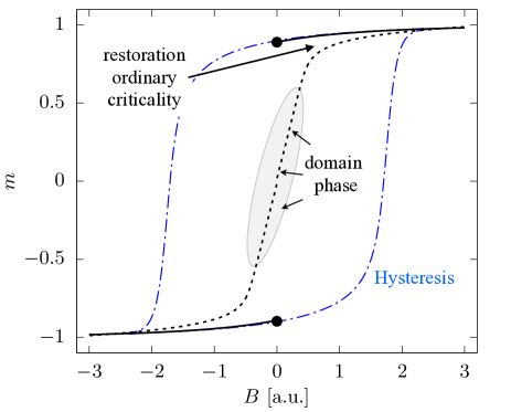
Figure 1: Magnetization $m$ normalized to its saturation value as a function of $B$. The solid and dashed lines represent the equilibrium curves in the absence and in the presence of dipolar interaction, respectively. The two bullets highlight the non-analyticity in $B=0$ expected only in the first case (see main text). The ellipse highlights the portion of the dashed curve corresponding to the multi-domain phase, while the arrow indicates the region where standard criticality ($M\sim B^{1/\delta}$ for $T\simeq T_{\rm c}$) is restored. The dot-dashed (blue) curve represents a prototypical hysteresis: both equilibrium scenarios – solid and dashed curves – are compatible with hysteresis.

When applied to the ferromagnetic-to-paramagnetic phase transition, these textbook cooperative models are compatible with low-temperature magnetization curves at thermodynamic equilibrium similar to the discontinuous curve in Fig. 1. The singularity in the magnetization curve originates from the very same non-analyticity that explains criticality and universality of critical exponents. In practical cases, the magnetization as a function of the external field $B$ does not jump from one branch to the other when $B=0$ is crossed: the system rather remains in a metastable configuration and the curve displays magnetic hysteresis, a typical out-of-equilibrium phenomenon (Fig. 1). In real magnets the short-ranged exchange interaction, which drives the establishment of ferromagnetism at low temperature, coexists with the long-ranged dipolar interaction. This second interaction generally frustrates the realization of a phase with uniform magnetization throughout a sample, consistently with the Griffiths’ theoremGriffiths (1968); Campa et al. (2014) for bulk magnets. The compromise most often encountered in experiments is the occurrence of a multi-domain phase (highlighted by the ellipse in Fig. 1). The discontinuity marked in Fig. 1 with two bullets on the equilibrium magnetization curve produced by models with short-ranged interactions only is replaced by an analytic function when dipolar interaction is taken into account.

A fundamental question then arises: along with the discontinuity in the equilibrium magnetization curve does dipolar interaction wipes away the critical behavior as well? In the following we consider a minimal model and show that the dipolar interaction acts as a relevant field, in the meaning of the renormalization group, beside the reduced temperature and the external $B$ fieldFisher (1974); Stanley (1999). This description is able to account for the coexistence of ordinary criticality with an analytic behavior of the magnetization as a function of $B$ at every temperature.
In section II we introduce the model and summurize the main experimental facts that inspired our study. In section III we propose a scaling ansatz that is validated in the forthcoming sections with a mean-field calculation (IV), a real-space renormalization group approach (V), and Monte-Carlo simulations (VI).

II Experimental facts and the model

In this paper we address properties related to thermodynamic equilibrium with particular focus on the behavior of the magnetization as a function of the applied field $B$. Magnetic hysteresis, usually considered the distinctive feature of the magnetization curve of ferromagnets, is not an equilibrium phenomenon and is, therefore, beyond our scope. Consistently with the scenario depicted in the introduction, the equilibrium magnetization for a real ferromagnet should behave smoothly as a function of the $B$ field when the latter passes from negative to positive values, without displaying any singularity at any temperature. The experimental validation of this fact is usually precluded because magnets are normally not able to relax to the configuration of minimal free energy within the measurement time. This means that magnetic hysteresis is also compatible with the vanishing of spontaneous magnetization at equilibrium prescribed by the Griffith’s theorem, as a result of dipolar frustration. Together with other coworkers, we recently reported an experimental study in which the magnetization of a ferromagnet strongly frustrated by dipolar interaction was measured in a wide range of temperature ($T$) and applied $B$ field, taking care that hysteretic effects were negligibleSaratz et al. (2016). This study was performed on Fe films epitaxially grown on Cu. For a thickness smaller than three atomic Fe layers these films are magnetized out of plane. In this configuration the frustrating effect of dipolar interaction against ferromagnetism is maximal because the dipolar interaction between any pair of magnetic moments in the film is antiferromagnetic. As a reference model for those Fe films we consider a 2D Ising Hamiltonian in which the usual nearest-neighbor ferromagnetic exchange interaction competes with an antiferromagnetic interaction decaying with the third power of the distance. This second term arises from the isotropic contribution to pairwise dipolar coupling, the anisotropic contribution vanishing exactly in films magnetized out of plane. The model Hamiltonian thus reads

$$H=-J\sum_{\langle i,j\rangle}S_{i}S_{j}+g\sum_{i\neq j}\frac{S_{i}S_{j}}{r^{3}_{ij}}-h\sum_{i}S_{i}$$ (1)

where $S_{i}=\pm 1$ are Ising spins disposed on a square lattice, representing the two out of plane directions along which magnetic moments preferentially point. The first sum runs over every distinct pair of nearest-neighboring sites (positive exchange coupling constant $J>0$ is assumed henceforth). The second sum, associated with dipolar interaction with strength $g>0$, runs now over every distinct pair of sites in the lattice. The last term represents the Zeeman energy $h=\mu B$, with $\mu$ magnetic moment. As a result of the competition between the short- and long-ranged interaction, this model exhibits modulated phases at low temperatures: striped phases at zero or small magnetic fieldsPighin and Cannas (2007); Vindigni et al. (2008) and bubble phases at intermediate fieldsPortmann et al. (2010); Diaz-Mendez and Mulet (2010); Cannas et al. (2011); Mendoza-Coto et al. (2015). Due to this feature this model and its generalized versions, in which the antiferromangetic coupling decays with a generic exponent, have been studied extensively during the last two decades in relation to the type of order realized in the modulated phases (smectic, Ising nematic, etc.) or to the possibility of producing self-generated glassinessSchmalian and Wolynes (2000); Nussinov (2004); Principi and Katsnelson (2016). The uniform phase can be enforced by applying a magnetic field larger that a certain threshold value $h_{\rm c}$, which is generally temperature dependentPortmann et al. (2010); Saratz et al. (2010). Whether some trace of the critical behavior, characterizing not frustrated models of ferromagnetism, is found in this uniform phase has eluded scientific interest so far. We remark that in the frustrated model the global magnetization is not an order parameter in the conventional understanding of second-order phase transitions. It is therefore a priori not obvious whether some critical behavior should be displayed at all in the uniform phase obtained when a large enough field is applied. The experiments on Fe films on Cu confirmed without any doubt that ordinary criticality indeed occurs in the uniform phase of a strongly frustrated ferromagnet. In that specific system the scaling behavior of the magnetization

$$m(\tau,B)=|\tau|^{\beta}\,F^{\pm}\left(\frac{B}{|\tau|^{\beta\delta}}\right)$$ (2)

($\tau=T/T_{\rm c}-1$) is realized when external fields larger than a certain temperature-dependent threshold ($B_{\rm c}$) are applied and is consistent with the critical exponents $(\beta,\delta)$ and scaling functions of the (unfrustrated) 2D Ising model. The threshold field $B_{\rm c}$ varies from few Gauss for $\tau<-0.05$ to about 50 Gauss ($5\times 10^{-3}$ T) around $T_{\rm c}$). In the – so-called – Griffiths-Widom representation power laws are obeyed up to eighty orders of magnitudeSaratz et al. (2016). The essence of the experimental observations on Fe films on Cu was confirmed by Monte-Carlo simulations performed using the Hamiltonian (1), even if realistic values of the Hamiltonian parameters could not be employed. For instance, using a physical value for the ratio $J/g$ ($\sim 500$) would produce magnetic domains of size larger than the accessible simulation boxes. Therefore, the much smaller ratio $J/g=10$ was used in order to observe both uniform and modulated phases in the same simulation. In experiments, the fields that suffice to stabilize the uniform phase correspond to a Zeeman energy of the order of $10^{-5}$ times $J$, while for the parameters used in Monte-Carlo simulations these fields are about $10^{-1}-10^{-2}$ times $J$ (see later on). Differently from what done in the analysis of experimental results, the critical exponents of the 2D Ising model were assumed in the analysis of Monte-Carlo results presented in Ref. Saratz et al., 2016. Therein, the scaling behavior (2) was verified adjusting the putative critical temperature $T_{\rm c}$ in order to obtain the maximal collapsing of simulated data. The critical temperature deduced in this way showed a linear dependence on the strength of dipolar coupling $g$:

$$T_{{\rm c},g}=T_{{\rm c},0}-11.3\,g$$ (3)

where $T_{{\rm c},0}=2J/(\ln(1+\sqrt{2}))\approx 2.269\;J$ is the Onsager critical temperature.

These experimental and numerical facts suggest that the scaling hypothesis reported in textbooks of magnetism should be phrased in more general terms.

III The scaling hypothesis

Both experimental and numerical evidence indicates that the critical behavior outside the multi-domain phase is controlled by the Onsager critical point, i.e. the critical point of the unfrustrated ferromagnet, ($g=0$) when $g/J\ll 1$. This fact provides a valuable hint to set the scaling hypothesis (2) in a broader framework. Concretely, it suggests to replace the scaling function $F^{\pm}(x)$, which depends on a single variable, by a two-variable scaling function $G^{\pm}(x,y)$. This allows accounting for an additional scaling field, parametrized by the variable $u=g/J$ henceforth, that acts as a relevant field for the unfrustrated critical point $(T=T_{{\rm c},0},B=0)$, in the sense of renormalization group. Hence, we might assume that the magnetization $m(\tau,b,u)$, is a generalized homogeneous function satisfying the relation

$$m(\lambda^{1/\beta}\tau,\lambda^{\delta}b,\lambda^{1/\omega}u)=\lambda\,m(\tau,b,u)\;\;\;\;\;\;\forall\lambda\neq 0$$ (4)

where $b=h/J=\mu\,B/J$ and $\omega$ is a new critical exponent. When $u=0$ we recover the behavior (2) from Eq. (4). Choosing $\lambda^{1/\omega}u=1$ we obtain the scaling form

$$m(\tau,b,u)=u^{\omega}G^{\pm}\left(\frac{|\tau|}{u^{\omega/\beta}},\frac{b}{u^{\omega\delta}}\right)$$ (5)

where $\pm$ refers to $\tau>0$ or $\tau<0$, respectively. The scaling functions $G^{\pm}(x,y)$ must satisfy some particular asymptotic behaviors. For instance, when $u\neq 0$ and $b\to 0$ the magnetization should vanish for any value of the temperature. From this follows the requirement

$$\lim_{y\to 0}G^{\pm}(x,y)=0.$$ (6)

Moreover, Eq. (2) must be recovered in the limit $u\to 0$ with $B$ finite, meaning that

$$G^{\pm}(x,y)\sim x^{\beta}F^{\pm}\left(\frac{y}{x^{\beta\delta}}\right)$$ (7)

for $x\gg 1$ and $y\gg 1$ with $y/x^{\beta\delta}$ finite. We then expect two different scaling regimes depending on whether

$$\begin{split}&b\ll b_{\rm c}\quad\Rightarrow\quad\text{multi-domain phase}\\ &b\gg b_{\rm c}\quad\Rightarrow\quad\text{ferromagnetic scaling region}\end{split}$$ (8)

the crossover field scaling with $u$ as $b_{\rm c}=h_{\rm c}/J\propto u^{\omega\delta}$. In the first regime the equilibrium magnetization is a smooth function (essentially a straight line for Fe films on Cu) of the applied field. In the second regime ($b\gg b_{\rm c}$) standard criticality expressed by Eq. (2) holds. Defining $p(y)\equiv G^{+}(0,y)=G^{-}(0,y)$, for $\tau=0$ one has

$$\frac{m}{u^{\omega}}=p\left(\frac{b}{u^{\omega\delta}}\right)\,.$$ (9)

Finally, to be compatible with Eq. (4) the singular part of the free energy must also be a generalized homogeneous function and satisfy the relation

$$f\left(\lambda^{\frac{1}{\beta(1+\delta)}}\tau,\lambda^{\frac{\delta}{1+\delta}}b,\lambda^{\frac{1}{\omega(1+\delta)}}u\right)=\lambda\,f(\tau,b,u)\;\;\;\;\;\;\forall\lambda\neq 0$$ (10)

In the next sections the validity of the scaling ansatz proposed in Eq. (4) will be confirmed studying the model (1) by means of different approaches: mean-field approximation, real-space renormalization group, Monte-Carlo simulations.

IV Mean-field theory

To analyze the mean-field approximation of Hamiltonian (1), we consider the Landau-Ginzburg (LG) free energy

$$F[\phi]=\frac{1}{2}\int d^{2}{\bf x}\left\{\left(J\,\nabla\phi({\bf x})\right)^{2}+r_{0}\phi^{2}({\bf x})+\frac{\bar{\lambda}}{2}\phi^{4}({\bf x})\right\}+\frac{g}{2}\int d^{2}{\bf x}\int d^{2}{\bf x}^{\prime}\frac{\phi({\bf x})\phi({\bf x^{\prime}})}{\left|{\bf x}-{\bf x}^{\prime}\right|^{3}}-h\int d^{2}{\bf x}\;\phi({\bf x})$$ (11)

where the scalar field $\phi({\bf x})$ represents the out-of-plane spin density in a magnetic thin film with easy axis perpendicular to the film plane. Space variables ${\bf x}$ and ${\bf x^{\prime}}$ are assumed to be dimensionless so that the constants $J$, $r_{0}$, $\bar{\lambda}$, and $h$ have the units of an energy. The terms between curly brackets model the ferromagnetic exchange interactions in the continuum limit. In the vicinity of the critical point one has

$$\begin{split}&r_{0}=T-T_{{\rm c},0}^{\rm MF}\\ &\bar{\lambda}=\frac{1}{3}T_{{\rm c},0}^{\rm MF}\end{split}$$ (12)

where $T_{{\rm c},0}^{\rm MF}$ is the mean-field transition temperature of the unfrustrated model (with $g=0$), for which the critical exponents are well-known: $\beta=1/2$ and $\delta=3$. Outside a limited region in the $(\tau,h)$ parameters space, i.e. for $h>h_{\rm c}$, domain states are not stable (they are either metastable or unstable) and the uniform solution $\phi=\phi_{0}$ is the equilibrium oneCannas et al. (2011). The saddle-point equation for $\phi_{0}$ is

$$(r_{0}+a_{g}\,g)\,\phi_{0}+\phi_{0}^{3}=h$$ (13)

where

$$a_{g}=\int\frac{d^{2}{\bf x}}{\left|{\bf x}\right|^{3}}\,.$$ (14)

One can implicitly assume a lower cutoff so that the integral above is not ill-defined. However, in the original functional (11) the dipolar interaction is well-defined in the domain of distributions. An explicit value can be assigned to the constant $a_{g}$ considering the coarse-grained (magnetostatic) description of the equivalent model, that is a slab of volume $V$ uniformly magnetized out of plane. For this system the demagnetizing energy is

$$\mathcal{E}_{\rm d}=\frac{1}{2}\mu_{0}M^{2}V=\frac{1}{2}\mu_{0}\mu^{2}\left(\frac{\phi_{0}}{a^{3}}\right)^{2}V\,.$$ (15)

In the last equivalence a cubic lattice of constant $a$ has been assumed as well as the obvious relation $M=\mu\,\phi_{0}/a^{3}$ between the macroscopic magnetization $M$ and the uniform spin density $\phi_{0}$ considered here. The demagnetizing energy in Eq. (15) should equal the corresponding contribution in the LG functional

$$\begin{split}F_{\rm d}[\phi]&=\frac{g}{2}\int d^{2}{\bf x}\int d^{2}{\bf x}^{\prime}\frac{\phi({\bf x})\phi({\bf x^{\prime}})}{\left|{\bf x}-{\bf x}^{\prime}\right|^{3}}\\ &=\frac{1}{2}\,\frac{\mu_{0}}{4\pi}\,\frac{\mu^{2}}{a^{3}}\,\phi_{0}^{2}\int d^{2}{\bf x}^{\prime}\int\frac{d^{2}{\bf x}}{\left|{\bf x}\right|^{3}}\end{split}$$ (16)

where in the second passage we have expressed the coupling constant $g$ in terms of the atomic magnetic moment and the lattice unit. A one-to-one mapping can now be established between individual terms in the Eqs. (15) and  (16)

$$\begin{split}&\frac{\mu}{a^{3}}\,\phi_{0}=M\\ &\mu\,\phi_{0}\int d^{2}{\bf x}^{\prime}=MV\\ &\frac{1}{4\pi}\int\frac{d^{2}{\bf x}}{\left|{\bf x}\right|^{3}}=1\,.\end{split}$$ (17)

Therefore, in this description, the constant in Eq. (14) is $a_{g}=4\pi$. From the saddle-point Eq. (13) associated with a uniform spin density $\phi_{0}$, we note that the presence of dipolar interaction effectively lowers the critical temperature by an amount $4\pi\,g$, namely

$$T_{{\rm c},g}^{\rm MF}=T_{{\rm c},0}^{\rm MF}-4\pi\,g\,.$$ (18)

Even if deduced in a mean-field context, the correction to the critical temperature provided by dipolar coupling is in excellent agreement with the results of Monte-Carlo simulations on a square lattice summarized in Eq. (3).

Let us go back to the main purpose of this section of verifying the validity of our scaling hypothesis within the mean-field approximation. To this aim, we define $z=\phi_{0}/u^{1/2}$ and divide both sides of the saddle-point Eq. (13) by $u^{3/2}$ to obtain

$$\left(a_{0}\frac{\tau}{u}+a_{1}\right)\,z+z^{3}=\frac{h}{u^{3/2}}$$ (19)

where $a_{0}$ and $a_{1}$ are numerical constants. Therefore, we obtain

$$\phi_{0}=u^{1/2}G^{\pm}\left(\frac{|\tau|}{u},\frac{h}{u^{3/2}}\right)$$ (20)

which is consistent with the scaling hypothesis proposed in (5), with a mean-field dipolar critical exponent $\omega=1/2$ characterizing the dipolar relevant field $u$.

V Real-space renormalization group approach (RSRG)

An fundamental requirement for the consistency of the scaling hypothesis in Eq. (4) is that the variable $u$ be a relevant field within a renormalization-group (RG) approach. In the following we demonstrate that this is indeed the case using the Niejmeijer and van Leeuwen RSRG techniqueNiemeijer and van Leeuwen (1973) and its extension to include long-range interactionsCannas (1995). For the sake of simplicity, we prove this only for the $B=0$ case, the extension to $B\neq 0$ being straightforward. Defining ${\cal H}\equiv-\beta H$, from Eq. (1) we have

$${\cal H}=K_{1}\sum_{\langle i,j\rangle}S_{i}S_{j}-K_{2}\sum_{i\neq j}\frac{S_{i}S_{j}}{r^{3}_{ij}}$$ (21)

namely, $K_{1}=\beta J$ and $K_{2}=\beta g$. We divide the system into Kadanoff Blocks with $\Lambda$ spins, so that the rescaling length of the RG transformation is $l=\sqrt{\Lambda}$. To each block $I$ we assign a block spin $S^{\prime}_{I}=\pm 1$. Defining the renormalized block Hamiltonian as

$${\cal H}^{\prime}=K^{\prime}_{1}\sum_{\langle I,J\rangle}S^{\prime}_{I}S^{\prime}_{J}-K^{\prime}_{2}\sum_{I\neq J}\frac{S^{\prime}_{I}S^{\prime}_{J}}{r^{3}_{IJ}}$$ (22)

where $r_{IJ}$ is the distance between blocks $I$ and $J$ measured in units of the rescaled length $l$, we obtained the recursion RG equations

$$K^{\prime}_{1} = K^{\prime}_{1}(K_{1},K_{2})$$

$$K^{\prime}_{2} = K^{\prime}_{1}(K_{1},K_{2})$$ (23)

for each block set. In Fig. 2 we show the different Kadanoff blocks used in the RG calculation. The details of the RG implementation are given in Appendix A.

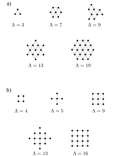
Figure 2: Kadanoff blocks for different values of $\Lambda$ used in the RG approach for (a) triangular lattice and (b) square lattice.

It is immediate to see that $K_{2}=0$ implies $K^{\prime}_{2}=0$. Therefore, the non-trivial fixed point of the RG equations (V) is located at $(K_{\rm c},0)$, with $K_{\rm c}$ determined by the equation $K^{\prime}_{1}(K_{\rm c},0)=K_{\rm c}$. In the RG approach, this fixed point corresponds to the critical temperature, i.e., $T_{\rm c,0}^{\rm RG}=J/k_{B}K_{\rm c}$ is the transition temperature of the unfrustrated model under the present approximation. Still in zero magnetic field, the RG equations linearized around this critical point are given by the matrix

$$\left(\begin{array}[]{cc}\frac{\partial K^{\prime}_{1}}{\partial K_{1}}&\frac{\partial K^{\prime}_{1}}{\partial K_{2}}\\ \frac{\partial K^{\prime}_{2}}{\partial K_{1}}&\frac{\partial K^{\prime}_{2}}{\partial K_{2}}\end{array}\right)_{K_{1}=K_{\rm c},K_{2}=0}=\left(\begin{array}[]{cc}\lambda_{\tau}&\frac{\partial K^{\prime}_{1}}{\partial K_{2}}\\ \frac{\partial K^{\prime}_{2}}{\partial K_{1}}&\frac{\partial K^{\prime}_{2}}{\partial K_{2}}\end{array}\right)_{K_{1}=K_{\rm c},K_{2}=0}$$

where $\lambda_{\tau}$ is the so-called thermal eigenvalue (see Appendix A). From Eq. (31) we have

$$\left.\frac{\partial K^{\prime}_{2}}{\partial K_{1}}\right|_{K_{1}=K_{\rm c},K_{2}=0}=0$$

and, therefore, the eigenvalue associated with the dipolar-coupling constant (in units of $k_{\rm B}T$) $K_{2}$ is given by

$$\lambda_{u}=\left.\frac{\partial K^{\prime}_{2}}{\partial K_{2}}\right|_{K_{1}=K_{\rm c},K_{2}=0}=\frac{1}{l^{3}}\,\left[M(K_{\rm c})\right]^{2}$$ (24)

where $M(K)$ is given in Eq. (34). It is also easy to see that the field eigenvalue is given by $\lambda_{b}=M(K_{\rm c})$.

The main idea behind the present approach is that eigenvalues of the RG equations linearized around a non-trivial fixed point that are larger than one correspond to relevant fieldsLe Bellac (1991); Fisher (1974); Stanley (1999). The aim of this section is, thus, to prove that $\lambda_{u}>1$. Typically, eigenvalues associated with relevant fields display a power-law dependence on the size of the Kadanoff blocks that are specific of the implemented renormalization procedureDelamotte (2012). The relative exponents are directly related to physical critical exponents (see below).

We calculated the eigenvalues for different values of $\Lambda$, both for the triangular and the square lattices shown in Fig. 2. Since the critical exponents are expected to be independent of the lattice structure, we could expect the general trend of the eigenvalues with $l$ to be the same for both lattices. We now make a change of variables from $(K_{1},K_{2})$ to $(\tau,u)$, with $u=K_{2}/K_{1}$, $\tau=K_{\rm c}/K_{1}-1$. Then, neglecting in first approximation the non-diagonal element of the RG matrix and assuming

$$\lambda_{\tau} \sim l^{y_{\tau}}$$

$$\lambda_{b} \sim l^{y_{b}}$$

$$\lambda_{u} \sim l^{y_{u}}$$

(where we have included now a finite magnetic field) it is easy to show that the singular part of the free energy should scale, close to the critical point, as

$$f(l^{y_{\tau}/d}\tau,l^{y_{b}/d}b,l^{y_{u}/d}u)\approx l\;f(\tau,b,u)\,,$$ (25)

with $d=2$ being the dimensionality of the system. Hence, comparing the equation above with Eq. (10) one obtains that

$$y_{\tau} = \frac{2}{\beta(1+\delta)}=\frac{1}{\nu}$$ (26)

$$y_{b} = \frac{2\delta}{1+\delta}$$ (27)

$$y_{u} \approx \frac{2}{\omega(1+\delta)}\,.$$ (28)

While the first two equations are well-known, to the best of our knowledge, the third Eq. (28) is not reported in the literature. This last equation allows relating the dipolar critical exponent $\omega$ to the other exponents.

As a consistency check of our RG approach, we first calculated $\lambda_{\tau}$ as a function of $l=\sqrt{\Lambda}$. Fig. 3a shows that $\lambda_{\tau}$ displays the expected power-law behavior (line in a log-log scale). A linear fitting combining the data for both the square and the triangular lattice yields the exponent $y_{\tau}=0.89$, reasonably close to the exact value $y_{\tau}=1$.

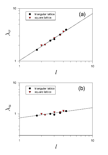
Figure 3: Thermal and dipolar eigenvalues vs. the scale length $l$. (a) $\lambda_{\tau}$. (b) $\lambda_{u}$

We then proceeded considering the behavior of the eigenvalue associated with the dipolar coupling, of our interest. Fig. 3b shows $\lambda_{u}$ as a function of $l$. As one can see, $\lambda_{u}$ is actually smaller than one for small values of $l$, because $\lambda_{u}=\lambda_{0}\,l^{y_{u}}$ with $\lambda_{0}<1$. However, also this eigenvalue clearly obeys a power-law behavior, which indicates that $\lambda_{u}$ becomes larger than one when sufficiently large Kadanoff blocks are consideredCannas (1995). In this sense, the crucial result of this section is that $y_{u}>0$, which confirms the assumption of $u$ being a relevant field. The exponent resulting from the fit of the $\lambda_{u}$ eigenvalues computed for different lattices is $y_{u}=0.33$. From Eqs.(26)-(28) this implies $\omega=1.015$. For completeness, it is worth mentioning that the same calculation for the field eigenvalue $\lambda_{b}$ yields a critical exponent $\delta=4.97$, very different from the exact result $\delta=15$. Hence, the value of $\omega$ resulting from this RG calculation can deviate significantly from the estimate of the same critical exponent obtained from Monte-Carlo simulations.

Finally, we note that the non–diagonal structure of the RG matrix implies that the eigenvectors associated with the eigenvalues $\lambda_{\tau}$ and $\lambda_{u}$ are actually not orthogonal. Taking this into accountNiemeijer and van Leeuwen (1973), would produce a correction in the critical temperature $T_{\rm c,0}^{\rm RG}=J/k_{B}K_{\rm c}$ which scales linearly with the strength of dipolar coupling $g$. Even without developing the calculation in details, the outcome would then be consistent with our Monte-Carlo and mean-field results (see Eqs. (3, 18)). A second consequence of the non–orthogonality of eigenvectors is a correction in Eq. (28), which could lead to an improved estimate of the critical exponent $\omega$.

VI Monte-Carlo simulations

Monte-Carlo (MC) simulations were performed using Hamiltonian  (1) on a square lattice comprising $N=L\times L$ sites, with $L=200$ for all simulations; periodic boundary conditions were assumed and handled implementing Ewald sums. We calculated the total magnetization $m=\sum\langle S_{i}\rangle/N$ (where $\langle S_{i}\rangle$ stands for the statistical average) as a function of $h$ at $T=T_{{\rm c},0}\approx 2.27J$ for $h>h_{\rm c}$ and different different values of $u=g/J$. The critical field $h_{\rm c}$ was estimated, either by direct calculation of the corresponding order parameters (for small values of $J/g$) or by a zero-field cooling – field-cooling procedure, as described in Ref. Saratz et al., 2016. At the beginning of each MC run we let the system equilibrate over $1000$ Monte-Carlo Steps (MCS) and then average over $1000$ sampling point taken every $100$ MCS along a single MC run.

In Fig.4a we show the simulated magnetization curves as a function of $h$ for different values of $J/g$ computed at $T=T_{{\rm c},0}$. In Fig.4b we show a scaling plot of $m/u^{\omega}$ vs. $h/u^{\omega\delta}$ for the same data set assuming $\omega\approx 1/10$ and $\delta=15$. The excellent collapsing of data confirms the scaling relation (9), which descends directly from the proposed scaling hypothesis (5).

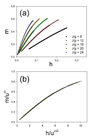
Figure 4: Monte-Carlo simulations for $L=200$, $T=T_{{\rm c},0}$ and different values of $J/g$. (a) Magnetization as a function of $h$. Data collapse of the same magnetization curves for $\omega=0.1\pm 0.002$ ($\delta=15$).

VII Discussion

We proposed an extension of the textbook scaling ansatz for ferromagnets that applies to the realistic situation in which the formation of magnetic domains – promoted by dipolar interaction – renders the Curie point technically unreachable. This ansatz is based on the assumption that the dipolar coupling acts as a relevant field, in the sense of renormalization group. This implies that a dipolar critical exponent $\omega$ needs to be introduced, besides the traditional ones related to the ferromagnetic-to-paramagnetic phase transition. The most reliable estimate of this exponent is the one resulting from Monte-Carlo simulations, i.e., $\omega\approx 1/10$. In fact, in this respect, the accuracy of mean-field theory and real-space renormalization-group approach is notoriously poor even for the unfrustrated modelLe Bellac (1991); Delamotte (2012). However, both these analytic approaches support the basic assumption of dipolar coupling being a relevant field.

Since dipolar interactions are ubiquitous and unavoidable in real magnets, our results suggest that long-range ferromagnetic order should be regarded as a crossover phenomenon. In other words, in the realm of equilibrium thermodynamics, the scaling behavior associated with the onset of long-range ferromagnetic ordering should be observable in the neighborhood of the putative critical point, but not too close to it. In fact, when the latter is approached by letting all the relevant fields $(\tau,b,u)$ go to zero, phases with modulated magnetization intervene that display a non-singular behavior of the ferromagnetic order parameter ($m$). In this perspective, our results reconcile the Griffith’s theoremGriffiths (1968); Campa et al. (2014) and dipolar frustration with the observation of criticality, at least for ferromagnetic films magnetized out of plane.

We hope that the present work will stimulate further investigations aimed at validating the proposed scaling hypothesis (5) for 3D magnets. Moreover, the model studied by us belongs to a more general class of models in which a generic exponent $\alpha$ is assumed for the power decay of the long-range interactionGiuliani et al. (2011, 2007); Mendoza-Coto et al. (2015); Grousson et al. (2000). The theoretical scenario of self-generated phase separation and avoided criticality was originally proposed for one of these models (with $\alpha=1$) in the context of high-$T_{\rm c}$ superconductorsTranquada et al. (1995); Emery and Kivelson (1993). The approach presented here could potentially help understand the complex phase diagram of this second class of materialsKeimer et al. (2015).

Appendix A Real-space renormalization group implementation

Following Niejmeijer and van Leeuwen prescription, we first divided the Hamiltonian (21) into two parts: ${\cal H}={\cal H}_{0}+{\cal V}$, where ${\cal H}_{0}=\sum_{I}{\cal H}_{0}^{I}$ and ${\cal V}=\sum_{I\neq J}{\cal V}_{IJ}$; ${\cal H}_{0}^{I}$ includes only the interactions between spins inside the block $I$, whereas ${\cal V}_{IJ}$ includes the interactions between spins belonging to different blocks $I$ and $J$. We also denoted $S_{i}^{I}$ ($i=1,\ldots,\Lambda$) the site spins belonging to the block $I$. The renormalized Hamiltonian (22), in the first order cumulant approximationNiemeijer and van Leeuwen (1973); Cannas (1995) is then given by

$${\cal H}^{\prime}=\sum_{I\neq J}\langle{\cal V}_{IJ}\rangle_{0},$$ (29)

where

$$\langle{\cal O}\rangle_{0}=\frac{1}{Z_{0}}\;{\rm Tr}_{\{S_{i}^{I}\}}P\left(\{S_{i}^{I}\},\{S^{\prime}_{I}\}\right)\,\exp\left[{\cal H}_{0}(\{S_{i}^{I}\})\right]\,{\cal O}$$ (30)

with

$$Z_{0}={\rm Tr}_{\{S_{i}^{I}\}}P\left(\{S_{i}^{I}\},\{S^{\prime}_{I}\}\right)\,\exp\left[{\cal H}_{0}(\{S_{i}^{I}\})\right]$$

and

$$P\left(\{S_{i}^{I}\},\{S^{\prime}_{I}\}\right)=\prod_{I}\,\frac{1}{2}\left[1+S^{\prime}_{I}\,{\rm sgn}\left(\sum_{i=1}^{\Lambda}S_{i}^{I}\right)\right]$$

is the weight function which characterizes the majority rule recipes. We will use this expression also when $\Lambda$ is an even number, meaning that $P$ assigns the values $S^{\prime}_{I}=\pm 1$ with probability $1/2$ to spins configurations with zero magnetization in the block. In particular, it is easy to see that $\langle S_{i}^{I}\rangle_{0}=a_{i}(\vec{K})\,S^{\prime}_{I}$, where $a_{i}(\vec{K})$ does not depend on the block $I$. Assuming now thatCannas (1995) $r_{ij}\approx l\,r_{IJ}$ for $r_{IJ}>1$, replacing into Eqs.(21) and (29), and comparing with Eq.(22), after some straightforward algebra we find

$$K^{\prime}_{2}=\frac{K_{2}}{l^{3}}\,\left[\sum_{i\in I}a_{i}(\vec{K})\right]^{2}$$ (31)

$$K^{\prime}_{1}=K_{1}\,\sideset{}{{}^{\prime}}{\sum}_{i\in I}\sideset{}{{}^{\prime}}{\sum}_{j\in J}a_{i}a_{j}-K_{2}\sum_{i\in I}\sum_{j\in J}\frac{1}{r_{ij}^{3}}a_{i}a_{j}+K^{\prime}_{2}$$ (32)

where $I$ and $J$ in the last equation are nearest-neighboring blocks. The first pair of sums (primed sums) in Eq.(32) run over nearest-neighboring sites $i$ and $j$, while the second pair run over all sites in both blocks. Other useful block dependent quantities were calculated, such as

$$L(K)\equiv\left.\sideset{}{{}^{\prime}}{\sum}_{i\in I}\sideset{}{{}^{\prime}}{\sum}_{j\in J}a_{i}a_{j}\right|_{K_{1}=K,K_{2}=0}$$ (33)

and

$$M(K)\equiv\left.\sum_{i\in I}a_{i}(\vec{K})\right|_{K_{1}=K,K_{2}=0}$$ (34)

For instance, the ferromagnetic (short range) critical point is determined by $L(K_{\rm c})=1$ and the corresponding thermal eigenvalue $\lambda_{\tau}=l^{1/\nu}$ by

$$\lambda_{\tau}=\left.\frac{\partial K^{\prime}_{1}}{\partial K_{1}}\right|_{K_{1}=K_{\rm c},K_{2}=0}=1+K_{\rm c}\left.\frac{dL}{dK}\right|_{K=K_{\rm c}}$$ (35)

We see that, to determine the stability of the ferromagnetic fixed point under the present approximation we just need the quantities

$$a^{\prime}_{i}(K)=a_{i}(K,0)=\left.\langle S_{i}^{I}\rangle_{0}\right|_{S^{\prime}_{I}=1,K_{1}=K,K_{2}=0}.$$ (36)

Let’s consider a simple example for $\Lambda=5$, which corresponds to a cross-shaped Kadanoff block (see Fig.2b). Suppose that we label $i=0$ the central site and $i=1,2,3,4$ the external sites of the block. By symmetry, the coefficients $a^{\prime}_{i}(K)=a_{e}(K)$, $i=1,2,3,4$, are all equivalent. Then from Eqs.(30) and (36) we obtain

$$a_{e}(K)=\frac{e^{4K}+e^{-4K}+2e^{2K}+2e^{-2K}}{6+e^{4K}+e^{-4K}+4e^{2K}+4e^{-2K}}$$ (37)

and for the central site

$$a^{\prime}_{0}(K)=\frac{6+e^{4K}-e^{-4K}+4e^{2K}-4e^{-2K}}{6+e^{4K}+e^{-4K}+4e^{2K}+4e^{-2K}}\,.$$ (38)

Between two neighboring blocks there are three first-neighbor bonds. Hence, $L(K)=3[a_{e}(K)]^{2}$ and $M(K)=4a_{e}(K)+a_{0}(K)$. For large clusters the functions $a_{i}(K)$ can be obtained with the aid of symbolic manipulation programs, for clusters of size up to $\Lambda\approx 20$ (see Fig.2).

References

- Taroni et al. (2008) A. Taroni, S. T. Bramwell, and P. C. W. Holdsworth, Journal of Physics: Condensed Matter 20, 275233 (2008).
- Stanley (1999) H. E. Stanley, Rev. Mod. Phys. 71, S358 (1999).
- Goldenfeld (1992) N. Goldenfeld, Lectures on phase transitions and the renormalization group, vol. 85 of Frontiers in physics (Perseus Books Publishing, Reading, Massachusetts, 1992).
- Le Bellac (1991) M. Le Bellac, Quantum and Statistical Field Theory, Oxford Science Publ (Clarendon Press, Oxford, 1991).
- Griffiths (1968) R. B. Griffiths, Phys. Rev. 176, 655 (1968).
- Campa et al. (2014) A. Campa, T. Dauxois, D. Fanelli, and S. Ruffo, Physics of Long-Range Interacting Systems (Oxford University Press, Oxford, 2014).
- Fisher (1974) M. E. Fisher, Rev. Mod. Phys. 46, 597 (1974).
- Saratz et al. (2016) N. Saratz, D. A. Zanin, U. Ramsperger, S. A. Cannas, D. Pescia, and A. Vindigni, Nat. Commun. 7, 13611 (2016).
- Pighin and Cannas (2007) S. A. Pighin and S. A. Cannas, Phys. Rev. B 75, 224433 (2007).
- Vindigni et al. (2008) A. Vindigni, N. Saratz, O. Portmann, D. Pescia, and P. Politi, Phys. Rev. B 77, 092414 (2008).
- Portmann et al. (2010) O. Portmann, A. Gölzer, N. Saratz, O. V. Billoni, D. Pescia, and A. Vindigni, Phys. Rev. B 82, 184409 (2010).
- Diaz-Mendez and Mulet (2010) R. Diaz-Mendez and R. Mulet, Phys. Rev. B 81, 184420 (2010).
- Cannas et al. (2011) S. A. Cannas, M. Carubelli, O. V. Billoni, and D. A. Stariolo, Phys. Rev. B 84, 014404 (2011).
- Mendoza-Coto et al. (2015) A. Mendoza-Coto, D. A. Stariolo, and L. Nicolao, Phys. Rev. Lett. 114, 116101 (2015).
- Schmalian and Wolynes (2000) J. Schmalian and P. G.Wolynes, Phys. Rev. Lett. 85, 836 (2000).
- Nussinov (2004) Z. Nussinov, Phys. Rev. B 69, 014208 (2004).
- Principi and Katsnelson (2016) A. Principi and M. I. Katsnelson, Phys. Rev. Lett. 117, 137201 (2016).
- Saratz et al. (2010) N. Saratz, A. Lichtenberger, O. Portmann, U. Ramsperger, A. Vindigni, and D. Pescia, Phys. Rev. Lett. 104, 077203 (2010).
- Niemeijer and van Leeuwen (1973) T. Niemeijer and J. M. J. van Leeuwen, Phys. Rev. 31, 1411 (1973).
- Cannas (1995) S. A. Cannas, Phys. Rev. B 52, 3034 (1995).
- Delamotte (2012) B. Delamotte, in Renormalization Group and Effective Field Theory Approaches to Many-Body Systems,, edited by J. Polonyi and A. Schwenk (Springer-Verlag, Berlin Heidelberg, 2012).
- Giuliani et al. (2011) A. Giuliani, J. L. Lebowitz, and E. H. Lieb, Phys. Rev. B 84, 064205 (2011).
- Giuliani et al. (2007) A. Giuliani, J. L. Lebowitz, and E. H. Lieb, Phys. Rev. B 76, 184426 (2007).
- Grousson et al. (2000) M. Grousson, G. Tarjus, and P. Viot, Phys. Rev. E 62, 7781 (2000).
- Tranquada et al. (1995) J. M. Tranquada, B. J. Sternlieb, J. D. Axe, Y. Nakamura, and S. Uchida, Nature 375, 561 (1995).
- Emery and Kivelson (1993) V. Emery and S. Kivelson, Physica C 209, 597 (1993), ISSN 0921-4534.
- Keimer et al. (2015) B. Keimer, S. A. Kivelson, M. R. Norman, S. Uchida, and J. Zaanen, Nature 518, 179 (2015).