The Long-Term Secular Mass Accretion Rate of the Recurrent Nova T Pyxidis

Abstract

We present Hubble Space Telescope ultraviolet spectroscopy of the recurrent nova T Pyxidis obtained more than 5 years after its 2011 outburst indicating that the system might not have yet reached its deep quiescent state. The ultraviolet data exhibit a 20% decline in the continuum flux from the pre-outburst deep quiescence state to the post-outburst near quiescent state. We suggest that a decline across each recurring nova eruption might help explain the proposed 2 mag steady decline of the system since 1866 (Schaefer et al., 2010). Using an improved version of our accretion disk model as well as International Ultraviolet Explorer ultraviolet and optical data, and the $4.8$ kpc distance derived by Sokoloski et al. (2013) (and confirmed by De Gennaro Aquino et al. (2014)), we corroborate our previous findings that the quiescent mass accretion rate in T Pyx is of the order of $10^{-6}M_{\odot}$yr^-1. Such a large mass accretion rate would imply that the mass of the white dwarf is increasing with time. However, with the just-release Gaia DR 2 distance of $\sim 3.3$ kpc (after submission of the first version of this manuscript), we find a mass accretion more in line with the estimate of Patterson et al. (2017), of the order of $10^{-7}M_{\odot}$yr^-1. Our results predict powerful soft X-ray or extreme ultraviolet emission from the hot inner region of the high accretion rate disk. Using constraining X-ray observations and assuming the accretion disk doesn’t depart too much from the standard model, we are left with two possible scenarios. The disk either emits mainly extreme ultraviolet radiation which, at a distance of 4.8 kpc, is completely absorbed by the interstellar medium, or the hot inner disk, emitting soft X-rays, is masked by the bulging disk seen at a higher inclination.

ApJ Accepted 1.0in

1 Introduction

Cataclysmic variables (CVs; see Warner (1995) for a review) are semi-detached interacting binaries with periods ranging from a fraction of an hour to days. In these systems a white dwarf (WD) primary accretes hydrogen-rich material from a secondary star filling its Roche-lobe. If the WD has a weak or negligible magnetic field, the matter is accreted onto the WD by means of an accretion disk. After enough material is accreted, the temperature and pressure at the base of accreted layer are high enough to trigger the CNO burning cycle of hydrogen, and the entire layer undergoes a thermonuclear runaway (TNR) known as the classical nova eruption (Schatzman, 1949; Paczynski, 1965; Starrfield et al., 1972). CVs for which more than one nova eruption has been observed are classified as recurrent novae (RNe). If the WD accretes more mass during quiescence than it ejects during classical nova eruptions, then it is believed that it might grow to reach the Chandraskhar limit and explode as a type Ia supernova (SN Ia; Whelan & Iben (1973); Nomoto (1982)). This is known as the single degenerate (SD) path to SN Ia, as opposed to the double degenerate (DD) scenario in which two CO WDs in a short period binary system merge (Webbink et al., 1984; Iben & Tutukov, 1984). CV systems, in theory, could also lead to SN Ia via the DD channel if they evolve into a double WD binary in which the total mass exceeds the Chandrasekhar limit and with a period shorter than $\sim 13$ hr (see Livio & Pringle (2011) for a review). Because of their massive WDs accreting at a high rate, RNe in general are considered to be ideal SN Ia progenitor candidates (SD channel) and for that reason they have been studied more extensively than other CVs.

1.1 The Prototypical Recurrent Nova T Pyxidis

T Pyx is a famous recurrent nova (RN), having erupted six times since 1890 (Waagan et al., 2011; Schaefer et al., 2013). With a recurrence time of only $\sim$20 years (though the last quiescence interval was twice as large, see Fig.1), the theory predicts that T Pyx must have a massive WD accreting at a high rate (Starrfield et al., 1985; Yaron et al., 2005). As it is often the case with systems that are extensively observed, more questions arise than are being solved, and T Pyx remains a poorly understood system.

T Pyx is surrounded by a nova shell remnant of ejected matter with a radius of 5 arcsec (Duerbeck & Seitter, 1979; Williams, 1982) as well as a faint outer halo twice as large (Shara et al., 1989). An analysis of the expanding knots in the nova shell (Schaefer et al., 2010) suggests that fast ejected material from the most recent RN eruptions is catching up and colliding with some slow moving material previously ejected in a classical nova eruption in 1866. Schaefer et al. (2010) further proposed that T Pyx was an ordinary CV until it underwent an eruption in 1866, increasing its accretion rate to a value several orders of magnitude larger than expected for its binary period. The enhanced mass transfer is believed to be due to a strong wind from the secondary star, itself driven by irradiation from the accretion-heated WD and inner disk (Knigge et al., 2000). This self-sustained feedback loop between the primary and secondary is believed to be a transient phase: as the accretion rate has been slowly declining, T Pyx has faded $\sim 2$ mag since its 1866 eruption (Schaefer et al., 2010). Some authors (Patterson et al., 1998; Knigge et al., 2000) have suggested that since 1866 (Schaefer et al., 2010) T Pyx might be in a super soft-Xray source (SSS) phase. However, Selvelli et al. (2008) exclude the presence of quasi-steady burning on the WD surface, and X-ray data (Greiner & Di Stefano, 2002; Selvelli et al., 2008; Balman, 2010) do not provide observational support for this scenario.

It is clear that during the long period of quiescence between the classical nova eruptions T Pyx is dominated by emission from its accretion disk and that the mass accretion rate is very high (Selvelli et al., 2008; Godon et al., 2014). In order to properly model the accretion disk, it is important to consider the binary system parameters, as the accretion disk model is defined by the mass of the central star, the radius of the central star (giving the lower limit for the inner radius of the disk), the binary separation (to help assess the outer radii of the disk), the inclination, and of course the mass accretion rate. Furthermore, as the theoretical spectrum is being scaled to the observed spectrum, the reddening as well as the distance to the system become the most important parameters of all.

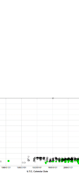
Figure 1: The AAVSO light curves of T Pyx, from 1965 to 2018, covering the last two eruptions (in 1966 and 2011). The visual magnitude ($m_{v}$, as seen by an actual observer, e.g. Stanton (1999); Bessel (2005)) is denoted with empty black circles, the standard Johnson V magnitude (Johnson & Morgan, 1953; Bessel, 2005) is denoted with filled green squares. With time, more Johnson V magnitude data have been collected by AAVSO members as CCDs have become easily available, cheaper and better. Both AAVSO light curves ($m_{v}$ and Johnson V) exhibit a very slight decrease in magnitude apparent from $\sim$1988 till about 2010. Note that the peak magnitude is almost exactly the same ($m_{v}\sim 6$) in both eruptions. Note: due to maximum size, Fig.1b in the ApJ version has been removed.

1.2 System Parameters

Table 1: T Pyxidis System Parameters

Parameter	Units	Value	References
$M_{\rm wd}$	$M_{\odot}$	0.7-1.35	Uthas et al. (2010); Starrfield et al. (1985); Webbink et al. (1987); Schaefer et al. (2010)
$R_{\rm wd}$	km	2000-8500	Assuming a 30,000 K WD with a mass $M_{\rm wd}=1.35M_{\odot}$ and $M_{\rm wd}=0.7M_{\odot}$, respectively.
$M_{2}$	$M_{\odot}$	0.12-0.14	Knigge et al. (2000); Uthas et al. (2010)
$R_{2}$	km	1.18$\times 10^{5}$	Knigge et al. (2000) ($R_{2}=0.17R_{\odot}$)
$i$	deg	10-30	Webbink et al. (1987); Uthas et al. (2010). Patterson et al. (2017) suggest $i\sim 50^{\circ}$-$60^{\circ}$
$d$	kpc	4.8$\pm 0.5$	Sokoloski et al. (2013); De Gennaro Aquino et al. (2014), Gaia DR2 data implies $d\sim 3.3$ kpc.
$P$	hrs	1.8295	Schaefer et al. (1992); Patterson et al. (1998); Uthas et al. (2010); Patterson et al. (2017)
$E(B-V)$		0.25-0.50	Gilmozzi & Selvelli (2007); Shore et al. (2013); Godon et al. (2014)
$a$	km	5-6$\times 10^{5}$	The values are for $M_{\rm wd}=0.7M_{\odot}$, and $M_{\rm wd}=1.35M_{\odot}$, respectively.

Distance

Until 5 years ago the distance to T Pyx was not known and it was assumed to be of the order of about 1 kpc to a few kpc, e.g. Selvelli et al. (1995) and Patterson et al. (1998) assumed 3.5 kpc. More recently Sokoloski et al. (2013) and De Gennaro Aquino et al. (2014) found a distance of 4.8-5.0 kpc (respectively), and after we submitted a first version of this manuscript, Gaia DR2 data (Prusti et al., 2016; Brown et al., 2018; Eyer et al., 2018) revealed a parallax of 0.305119199 mas with an error 0f 0.041850770 mas, giving a distance of 3,277 pc (between 2,882 pc and 3,798 pc). This is the reason why in a preliminary analysis of the archival International Ultraviolet Explorer (IUE) spectra of T Pyx, we assumed a distance of 1 kpc (and reddening of $E(B-V)=0.25\pm 0.05$), and found a mass accretion rate of only $10^{-8}M_{\odot}$yr^-1 (Sion et al., 2010). In our more recent analysis, assuming $d=4.8$ kpc (and $E(B-V)=0.35\pm 0.05$) we found a mass accretion rate two orders of magnitude larger (Godon et al., 2014). In the present work, we initially assumed $d=4.8$ kpc, but then we took into account the just-released distance from Gaia DR2, which brings the mass accretion of T Pyx closer to $10^{-7}M_{\odot}$yr^-1. This demonstrates the importance of the distance (and reddening, see below) to determine the correct mass accretion rate of the system.

Reddening

At a distance of a few kpc, and with a galactic extinction of $E(B-V)=0.25$ in that direction (Schlegel et al., 1998) , one can expect the reddening towards T Pyx to be at least of that same order of magnitude, namely $E(B-V)\sim 0.25$ or larger. Indeed, using co-added and merged IUE (SWP+LWP) spectra (with the latest improved data reduction) of T Pyx and adopting the extinction curve of Savage & Mathis (1979), Gilmozzi & Selvelli (2007) obtained $E(B-V)=0.25\pm 0.02$ from the 2175 Å dust absorption feature (“bump”). On the other hand, however, using diffuse interstellar bands, Shore et al. (2011) found an extinction of $E(B-V)=0.49\pm 0.17$, basically double that found by Gilmozzi & Selvelli (2007). Since an error of 0.05 in $E(B-V)$ (which is quite typical for CV: Verbunt (1987)) can produce a change in the UV flux of $\sim$20% at 3000 Å and as much as $\sim$50% at 1300 Å , the large discrepancy between the derived values of $E(B-V)$ for T Pyxidis is frustrating. The matter is further complicated by the fact that deriving the reddening from the 2175 Å bump is accurate to within about 20% and the extinction curve itself is an average throughout the Galaxy and could be different in different directions (Fitzpatrick, 1999). If the reddening towards T Pyxidis is larger than the Galactic reddening in that direction (i.e. $E(B-V)>0.25$), then the obvious culprit is obscuration by the material that has repeatedly been ejected during the recurring nova eruptions. Whether the ‘extinction properties’ of the ejected material are identical to those of the Galactic ISM is also questionable. It is, therefore, safe to assume for T Pyxidis a reddening value $E(B-V)=0.35_{-0.10}^{+0.15}$. It is within this context of uncertainty that in Godon et al. (2014) we carried out a UV spectral analysis assuming different values for $E(B-V)$, ranging from 0.25 to 0.50 (even though we derived $E(B-V)=0.35\pm 0.05$ using the 2175 Å feature from the combined and merged IUE and Galaxy Evolution Explorer (GALEX) spectra).

We have updated our dereddening software and in the present work we carry out a new estimate of the reddening giving $E(B-V)=0.30\pm 0.05$ (see Section 3.2). Our results for this value of $E(B-V)$ are completely consistent with our previous results in Godon et al. (2014).

Disk Models and Mass Accretion Rates

A mass accretion rate of $\sim 10^{-8}M_{\odot}$yr^-1 was derived by Selvelli et al. (2008) by scaling the flux of two Wade & Hubeny (1998) disk models at 1600 Å. A first model had $M_{\rm wd}=1.03M_{\odot}$ with $\dot{M}=10^{-8}M_{\odot}$yr^-1, and the second model had $M_{\rm wd}=1.21M_{\odot}$ with $\dot{M}=10^{-8.5}M_{\odot}$yr^-1. However, the flux at a given wavelength for a given mass accretion rate and a given WD mass cannot be scaled to much higher values of $\dot{M}$ and larger $M_{\rm wd}$ (e.g. $1.35M_{\odot}$), as the Planckian peak moves to shorter wavelengths with increasing values of $\dot{M}$ and $M_{\rm wd}$. Instead, one should rather use a realistic accretion disk model for the values of $\dot{M}$ and $M_{\rm wd}$ in question and fit the entire wavelength range rather than one given wavelength (which at 1600 Å doesn’t include the FUV spectrum). Furthermore, the size of the accretion disk in T Pyx is such that the truncation of the outer disk, either due to tidal forcing (near $\sim 0.3a$, where $a$ is the binary separation) or just to the size of the Roche lobe ($\sim 0.6a$), has to be taken into account. In our accretion disk models, the outer disk has a lower temperature, significantly contributing to the UV and optical ranges, while the inner disk contributes to the EUV (especially at the higher mass accretion rate inferred from the data). In the present work we take the inner and outer radius of the disk into account to generate realistic disk models. Our models (see section 3, Table 4) have an outer disk temperature of $\sim$20,000 K and $\sim$40,000 K which is hotter than the $\sim$10,000 K models of Wade & Hubeny (1998) used by Selvelli et al. (2008), and therefore have a smaller outer radius and provide less flux for the same $\dot{M}$ justifying our higher $\dot{M}$ results.

Inclination

It has been shown that the inclination of the binary system is possibly low, somewhere between 10^∘ to 30^∘, based on the narrow nearly stationary emission lines (Webbink et al., 1987; Uthas et al., 2010). However, Patterson et al. (2017) suggest a higher binary inclination $i\approx 50-60^{\circ}$, as inferred from Hubble Space Telescope (HST) imaging and radial velocities of the 2011 ejected shell, as well as from the soft X-ray eclipse (Tofflemire et al., 2013), interpreting the emission lines as arising in an accretion disk wind (Sokoloski et al., 2013). While, it is possible for strong X-ray modulation to occur even at low inclination, as is the case for BG CMi (Hellier et al., 1993) with $i\approx 30^{\circ}$ (maybe due to stream disk overflow falling to smaller radii near the WD itself), we consider here also a larger inclination to check how this assumption affects our results (we generate disk models assuming $i=20^{\circ}$ and $i=60^{\circ}$).

The WD and Secondary

Because of the short recurrence time and large $\dot{M}$ between the classical nova eruptions, it is expected, on theoretical grounds, that the WD in the system be massive, close to $1.35M_{\odot}$ (Starrfield et al., 1985; Webbink et al., 1987; Schaefer et al., 2010). However, in their optical radial velocity study of emission line velocities, Uthas et al. (2010) derived a mass ratio of $q=0.20$ and an inclination of $i=10^{\circ}$, and, assuming a $0.14M_{\odot}$ for the secondary, they inferred a WD mass as low as $0.7M_{\odot}$. Consequently, in the present work we consider both options: $M_{\rm wd}=0.70M_{\odot}$ and $1.35M_{\odot}$. The radius of the WD is then taken directly from the mass-radius relation for a non-zero temperature WD (e.g. Woods (1995)): $\sim$8500 km for a $0.7M_{\odot}$ mass, and $\sim$2000 km for $1.35M_{\odot}$ mass, assuming that the WD has a temperature of 30,000 K. As to the secondary its mass is not known, but it has been estimated to be as low as $0.06M_{\odot}$ for a high inclination (Patterson et al., 2017), and as large as $0.3M_{\odot}$ (see Selvelli et al. (2008) for a review). In the following we will assume that the secondary mass is $\approx 0.13M_{\odot}$ (Knigge et al., 2000; Uthas et al., 2010). We also assume that the radius of the secondary is its Roche lobe radius. Since the secondary mass and radius do not significantly affect the disk parameters, we do not consider here different values.

The Binary Separation

In order to model the disk, we need to know its size and therefore the binary separation. Using Kepler’s Law we find a binary separation $a\approx 5\times 10^{5}$ km assuming a $0.7M_{\odot}$ WD mass, and $a\approx 6\times 10^{5}$ km for a $1.35M_{\odot}$ WD mass, corresponding to $0.72R_{\odot}$ and $0.86R_{\odot}$ respectively.

In the present work, using the Sokoloski et al. (2013)’s distance of 4.8 kpc we confirm our previously derived mass accretion rate of $\dot{M}\sim 10^{-6}M_{\odot}$ (Godon et al., 2014) with our newly improved synthetic disk spectra to model the ultraviolet (UV) spectra of T Pyx obtained during quiescence (pre- and post-outburst). However, using the Gaia DR2 data, we derive a distance of 3.3 kpc, which lowers the mass accretion rate to the order of $10^{-7}M_{\odot}$yr^-1. We further extend our analysis into the optical and find that our results are not inconsistent with the optical data. The UV data further show that the mass accretion rate has slightly decreased 4 years after the outburst in comparison to its pre-outburst value. We present the data in Section 2, give an overview of our spectral modeling in Section 3, present the results in Section 4 and discuss them in Section 5, and we conclude in Section 6 with a short summary.

2 IUE Archival Data and HST Observations

2.1 The Pre-outburst, Outburst, and Decline UV Spectra

There are 58 pre-outburst IUE spectra of T Pyx which were collected between 1979 and 1996 (Szkody et al., 1991; Gilmozzi & Selvelli, 2007; Selvelli et al., 2008) consisting of 17 spectra with wavelength coverage 1851-3300 Å  (LWP) and 31 spectra with wavelength coverage 1150-1978 Å  (SWP). Of these, one spectrum (1979) seems to be off target, and several others are spectra of the background sky near T Pyx. Consequently, in the present work we use 36 SWP spectra together with 14 LWP spectra obtained over a period of 17 years (1980-1996, see Table 2), exhibiting the same continuum flux level within $\pm$9%. The 9% fluctuation in the continuum flux level is detected on a time scale as small as $\sim$1 day and could be due, for example, to a hot spot, and/or to the stream-disk material overflowing the disk and partially veiling the accretion disk at given orbital phases. Since this fluctuation in flux is not very large and the S/N of each individual spectrum is rather low, we carry out the same procedure as in Godon et al. (2014) and combine these spectra together to obtain a pre-outburst spectrum of T Pyx that can be used to assess the continuum flux level change of the post-outburst spectra. Details of IUE exposures are listed in Table 2 (in chronological order) together with a GALEX pre-outburst spectrum obtained in 2005.

T Pyx was later observed with HST/Space Telescope Imaging Spectrograph (STIS) ($\sim$1150-2900 Å) first during its outburst while the spectrum was dominated by broad and strong emission lines with a flux level 10-100 times larger than in quiescence (Shore et al., 2013; De Gennaro Aquino et al., 2014), then with STIS and the Cosmic Origins Spectrograph (COS) ($\sim$900-1725 Å) during its late decline from outburst (Godon et al., 2014; De Gennaro Aquino et al., 2014) as its flux level reached its pre-outburst value and the emission lines almost vanished, and more recently with COS ($\sim$900-2150 Å) as the system continues to decline (as reported here, see next subsection) with a continuum flux level slightly below its pre-outburst spectrum. The observation log of the HST post-outburst exposures is listed in Table 3 (also in chronological order). Each HST spectrum consists of several exposures obtained successively. For that reason in Table 3 we mark in bold the date of the first exposure to help differentiate between the actual spectra obtained at different epochs.

Table 2: T Pyxidis Pre-Outburst UV Archival Spectra

Telescope	Data ID	Date (UT)	Time (UT)	Exp. Time
		yyyy-mm-dd	hh:mm:ss	seconds
IUE	SWP08973	1980-11-05	04:09:56	12900
IUE	SWP29318	1986-09-27	18:22:55	16200
IUE	SWP32218	1987-11-02	12:12:44	16800
IUE	SWP32899	1988-02-11	07:27:19	12780
IUE	SWP33034	1988-03-03	04:29:13	23580
IUE	SWP34696	1988-11-05	14:01:04	17160
IUE	SWP37536	1989-11-07	14:12:10	16800
IUE	SWP43442	1991-12-22	10:20:50	15600
IUE	SWP44182	1992-03-16	03:55:48	15000
IUE	SWP44948	1992-06-17	22:09:41	16800
IUE	SWP46605	1992-12-28	12:15:49	16320
IUE	SWP47057	1993-02-27	06:09:34	16500
IUE	SWP47323	1993-03-20	04:47:40	20100
IUE	SWP47328	1993-03-21	05:30:39	18000
IUE	SWP47332	1993-03-22	04:05:15	23100
IUE	SWP49365	1993-11-29	11:49:59	9600
IUE	SWP49366	1993-11-29	15:25:32	10680
IUE	SWP50099	1994-02-24	06:07:47	11400
IUE	SWP50100	1994-02-24	09:47:40	10800
IUE	SWP50596	1994-04-20	01:58:50	24480
IUE	SWP52886	1994-11-23	12:27:47	9000
IUE	SWP52887	1994-11-23	15:52:41	9480
IUE	SWP53810	1995-02-02	04:04:13	11400
IUE	SWP54590	1995-05-03	23:48:06	11100
IUE	SWP54591	1995-05-04	03:30:52	11700
IUE	SWP56240	1995-11-26	19:15:40	12000
IUE	SWP57030	1996-05-01	23:24:57	12000
IUE	SWP57031	1996-05-02	03:10:44	12600
IUE	SWP57032	1996-05-02	23:16:03	12000
IUE	SWP57033	1996-05-03	03:04:57	12000
IUE	SWP57034	1996-05-03	08:05:54	10800
IUE	SWP57035	1996-05-03	13:03:18	6600
IUE	SWP57039	1996-05-04	03:19:54	7799
IUE	SWP57042	1996-05-04	09:41:57	9899
IUE	SWP57047	1996-05-05	02:23:20	10800
IUE	SWP57055	1996-05-06	03:05:51	10800
IUE	LWR07724	1980-11-05	02:08:20	7200
IUE	LWP09204	1986-09-27	16:15:42	7200
IUE	LWP11996	1987-11-02	17:00:13	6600
IUE	LWP12644	1988-02-11	05:20:34	7200
IUE	LWP12791	1988-03-03	07:29:37	12780
IUE	LWP14383	1988-11-05	11:44:47	7800
IUE	LWP16757	1989-11-07	11:52:47	7800
IUE	LWP22052	1991-12-22	14:45:26	7200
IUE	LWP22608	1992-03-15	08:09:57	9600
IUE	LWP23317	1992-06-18	02:54:33	6900
IUE	LWP24612	1992-12-28	09:48:28	8400
IUE	LWP25020	1993-02-27	10:55:54	6600
IUE	LWP32286	1996-05-05	13:37:15	5700
IUE	LWP32287	1996-05-06	11:26:01	6600
GALEX	GI2_023004_T_PYX	2005-12-20	03:30:05	880

Table 3: T Pyxidis Post-Outburst HST Spectra

HST	Filters	Central	Data ID	Date (UT)	Time (UT)	Exp.Time
Instrument	Gratings	Wavelength		yyyy-mm-dd	hh:mm:ss	seconds
STIS	E140M	1425	obg101010	2011-05-07	08:01:44	571
STIS	E230M	1978	obg101020	2011-05-07	08:26:53	571
STIS	E140M	1425	obg199010	2011-07-28	18:52:15	285
STIS	E230M	1978	obg199020	2011-07-28	19:03:07	285
STIS	E140M	1425	obg103010	2011-10-04	12:56:11	285
STIS	E230M	1978	obg103020	2011-10-04	13:14:18	285
STIS	E140M	1425	obx701010	2012-03-28	15:25:23	2457
STIS	E140M	1425	obx701020	2012-03-28	16:50:44	3023
COS	G130M	1055	lbx702ouq	2012-03-28	18:36:38	461
COS	G130M	1055	lbx702owq	2012-03-28	18:47:22	461
COS	G130M	1055	lbx702oyq	2012-03-28	18:58:06	461
COS	G130M	1055	lbx702p0q	2012-03-28	19:08:50	461
STIS	E140M	1425	obxs01010	2012-12-21	05:18:19	2449
STIS	E140M	1425	obxs01020	2012-12-21	06:43:06	3015
COS	G130M	1055	lbxs02010	2012-12-21	08:31:37	1744
STIS	E140M	1425	obxs03010	2013-07-26	08:36:35	2449
STIS	E140M	1425	obxs03020	2013-07-26	09:57:04	3015
COS	G130M	1055	lbxs04010	2013-07-26	11:46:49	1744
COS	G140L	1105	lcue01010	2015-10-13	00:00:16	788
COS	G130M	1055	lcue01020	2015-10-13	01:20:11	3466
COS	G140L	1105	lcue02010	2016-06-01	02:14:18	788
COS	G130M	1055	lcue02020	2016-06-01	03:41:58	3466

The first 6 HST spectra (obtained between May 2011 and July 2013) were presented and analyzed in Godon et al. (2014) and De Gennaro Aquino et al. (2014) and showed that by December 2012 the continuum flux level had reached its pre-outburst value (see Fig.2), and remained constant thereafter (the July 2013 spectrum was basically identical to the December 2012 spectrum). The AAVSO light curve of the system also indicated that by $\sim$2013 the light curve had reached its quiescence level. The system, therefore, seemed to have returned to exactly the same quiescent state. The Dec 2012 and Jul 2013 post-outburst HST spectra agree very well with the pre-outburst IUE and GALEX spectra, as shown in Fig.3 (except for detector edge noise in GALEX and IUE). As a result of this, in Godon et al. (2014) we modeled the combined HST and IUE spectra with an accretion disk, yielding a mass accretion rate $\dot{M}\approx 2\pm 1\times 10^{-6}M_{\odot}$yr^-1.

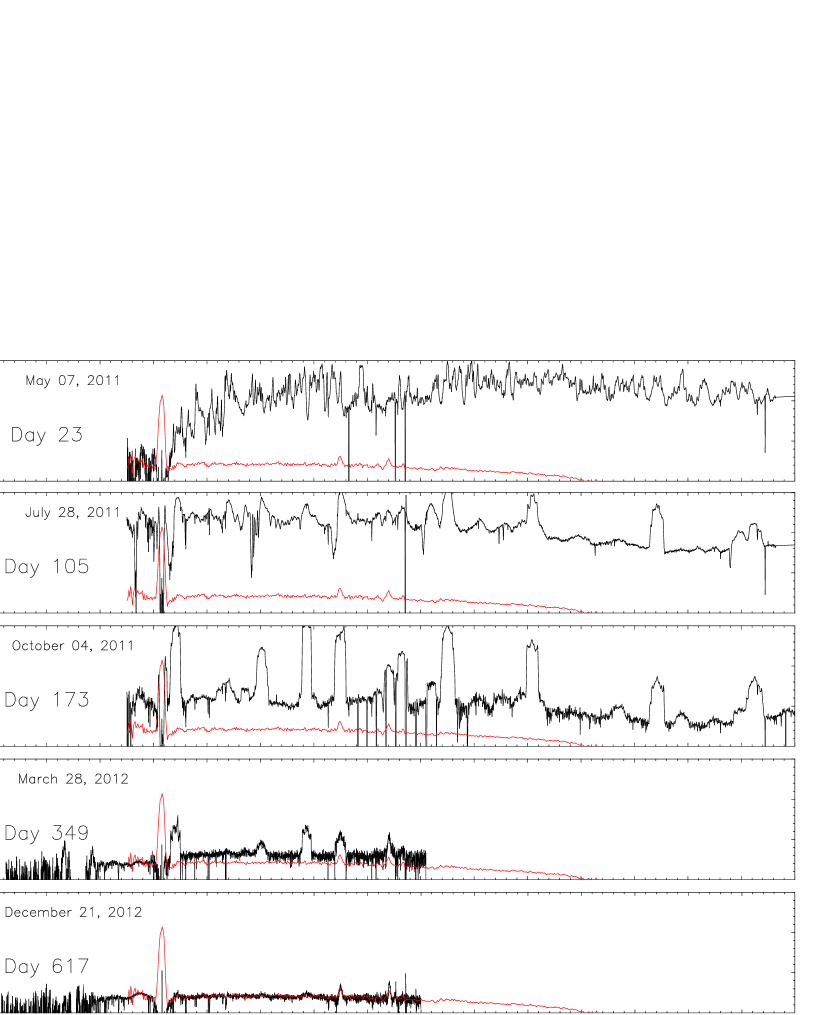
Figure 2: T Pyxidis decline from outburst. The first five HST spectra of T Pyx (as listed in Table 3) obtained as the system declined from its original eruption are shown in chronological order from top to bottom (solid black lines). The flux is given in log of erg s^-1cm^-2Å^-1 and the wavelength is in Å. The observation date and the number of days since eruption are indicated on the left in each panel. The pre-eruption IUE spectrum (generated from the co-added and combined IUE datasets listed in Table 2) is shown in red for comparison. The HST December 21, 2012 observations reveal a UV spectrum almost identical to the IUE pre-eruption spectrum (bottom panel).

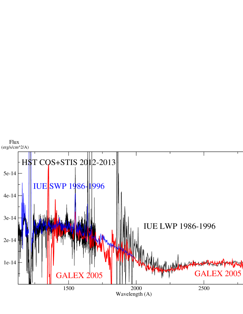
Figure 3: The pre-eruption combined (SWP and LWP) IUE spectra are shown together with the GALEX spectrum and the post-eruption HST spectra. All the spectra are color-coded and the observations years are indicated as marked. For a better contrast, and since they do not overlap, both the HST spectrum (in the short wavelengths) and IUE LWP spectrum (in the longer wavelengths) have been set to black. The S/N of the IUE LWP spectrum is very low and deteriorates toward the edges (as seen below 2000 Å). The GALEX spectrum (two spectral segments in red) presents a similar low S/N at its edges (including where the two segments meet around 1700-2000 Å). In spite of this, all the spectra agree relatively well in the regions where the S/N is good.

2.2 The 2015 & 2016 Late Decline/Quiescent HST/COS Spectra

We obtained two additional HST/COS far ultraviolet (FUV) spectra: the first one more than two years after the last HST spectrum, namely in October 2015, and the second one in June 2016.

For each two-orbit observation, we used two different FUV COS configurations - each taking one orbit and in time tag mode. In the first orbit, COS was configured with the G140L grating centered at 1105 Å, from which we extracted one spectral segment from 1150 Å to 2150 Å. In the second orbit, we used the G130M grating centered at 1055 Å, from which we extracted two spectral segments from 900 Å to 1045 Å and from 1055 Å to 1200 Å. The data were collected through the primary science aperture (PSA) of 2.5 arcsec diameter, and processed with CALCOS version 3.1.8 (Hodge et al., 2007; Hodge, 2011) through the pipeline, which produces, for each HST orbit, four sub-exposures generated by shifting the position of the spectrum on the detector by 20 Å each time. This strategy is used to reduce detector effects associated with COS. A description of the COS four positions sub-exposures and detector artifacts can be found in Godon et al. (2017a). For the first orbit (COS G140L 1105) the effective good exposure time of each sub-exposure was a little less than $\sim$200 sec. For the second orbit (COS G130M 1055) the exposure time for each sub-exposure was $\sim 866$ sec. The resulting spectrum covers the Lyman series down to its cut-off wavelength, including the L$\alpha$ region. Due to detector artifacts (especially near the edges), the resulting spectrum is not very reliable in the region where the segments overlap (1150-1200 Å) and in the shortest wavelengths ($<1000$ Å, see Figs.4a & b).

The October 2015 spectrum exhibits a net drop (of $\sim 20$%) in the continuum flux level when compared to the Dec 2012 - Jul 2013 HST spectra and IUE pre-outburst spectrum (see Fig.4a). The June 2016 spectrum has a continuum flux slightly higher than the October 2015 spectrum, but still well below the pre-outburst level (see Fig.4b).

To better emphasize the continuum flux changes, we average the spectra over the wavelength region 1400 Å - 1700 Å, omitting the emission lines. Namely, the averaged flux is given by

$$\frac{1}{\lambda_{2}-\lambda_{1}}\int_{\lambda_{1}}^{\lambda_{2}}F_{\lambda}d\lambda$$

with $\lambda_{1}=1400$ Å and $\lambda_{2}=1700$ Å. We present the averaged UV flux of the pre-outburst (IUE +GALEX) and post-outburst (HST) spectra in Fig.5. The first obvious behavior is the 9% fluctuation in the flux level seen in the IUE data and present even on a time-scale of $\sim 1~{}$day (year 1996). The GALEX flux data point, obtained at the end of 2005, is rather low, but not inconsistent with the IUE data. The HST post-eruption data show that the Dec 2012 and Jul 2013 data points fall within the range of values of the pre-outburst IUE data and explain how they were interpreted as the system having come back to its exact pre-eruption quiescent state (Godon et al., 2014). Only the October 2015 and June 2016 data points reveal that the system has apparently not yet reached quiescence and the UV continuum flux level is still decreasing. The 2016 data point seems to bounce back compared to the 2015 data point, however it can be understood as a ‘normal’ modulation of the continuum flux level, namely within the $\pm 9$% fluctuation. Both the 2015 and 2016 data points (with $F_{\lambda}\approx 2\times 10^{-14}$erg s^-1cm^-2Å^-1) are definitely below the averaged flux level of the pre-outburst data (with $F_{\lambda}\approx 2.5\times 10^{-14}$erg s^-1cm^-2Å^-1), showing a drop of $\sim 20$%. At this stage, it is not clear whether the system has reached quiescence or will decline further.

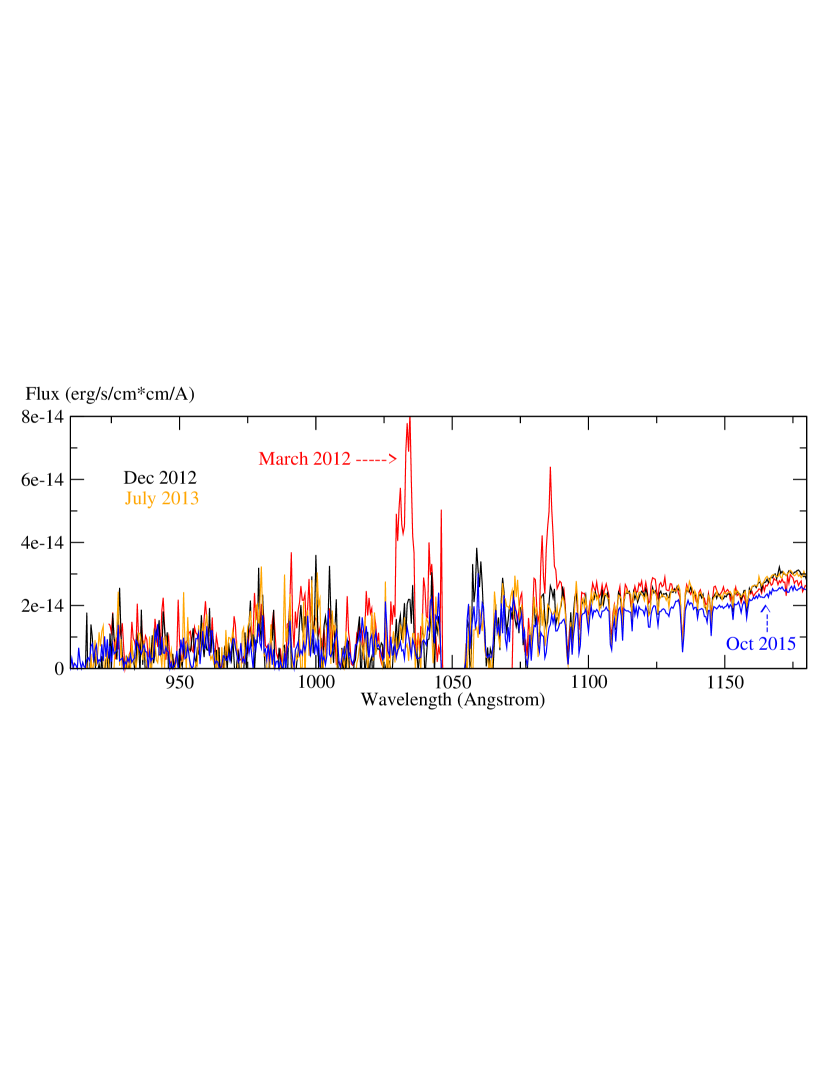
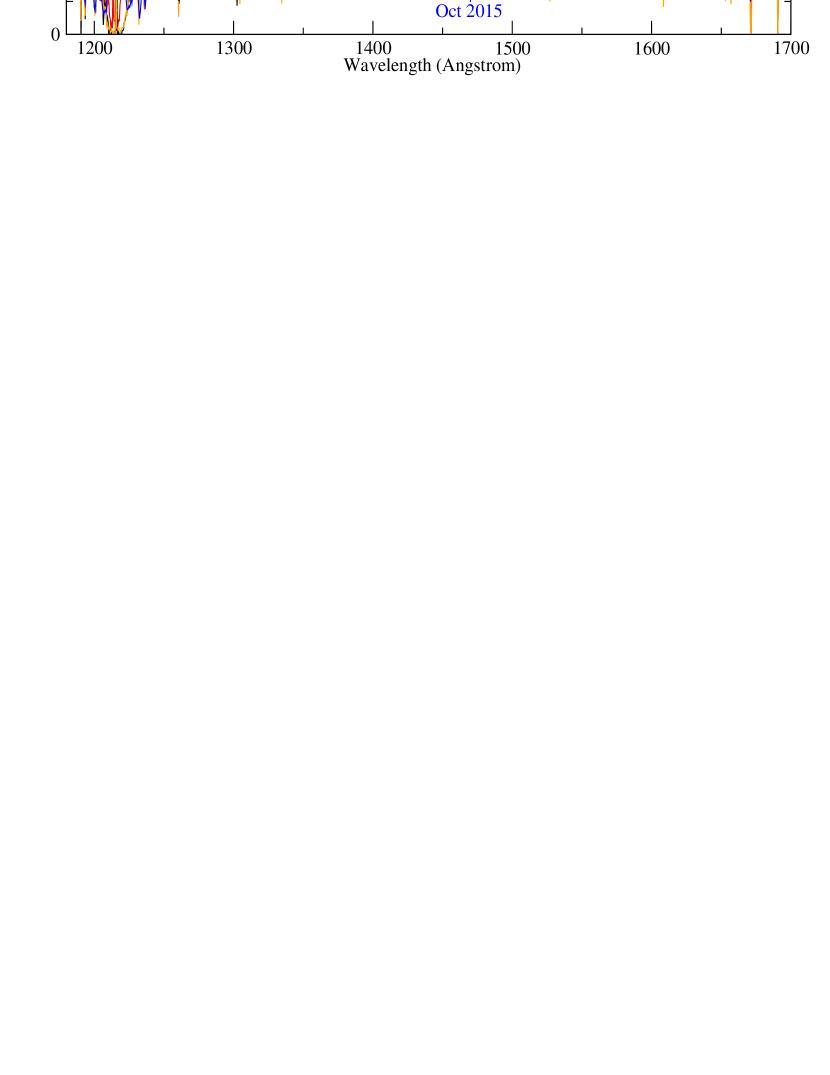
Figure 4a: The 2012, 2013 and 2015 HST FUV spectra of T Pyxidis are displayed showing the late decline of the system into quiescence. The first panel shows the COS G130M (1055 Å) spectra going down to the Lyman limit, but with a very low S/N (some of the flux below 1000 Å is actually negative, a sign that it is unreliable). In the short wavelengths the spectra have about the same continuum flux level, except for the March 2012 spectrum exhibiting a couple strong emission lines. The Oct 2015 spectrum has a slightly lower continuum flux level above 1000 Å. In panel (b) we show three STIS E140M (centered at 1425 Å) and one COS G140L (centered at 1105 Å) spectra (see Table 3). The March 2012 spectrum shows strong emission lines and has a continuum flux level significantly larger than the other spectra. The Oct 2015 spectrum shows a net decline in the continuum flux level. For most part, the Jul 2013 and Dec 2012 spectra are indistinguishable. The epochs are color-coded and indicate a further decrease in flux below the pre-eruption level for the data obtained after 2013. Note that the fluxes in the region where the STIS and COS spectra overlap ($\sim 1150$-1200 Å ) do not agree, especially for the March 2012 dataset.

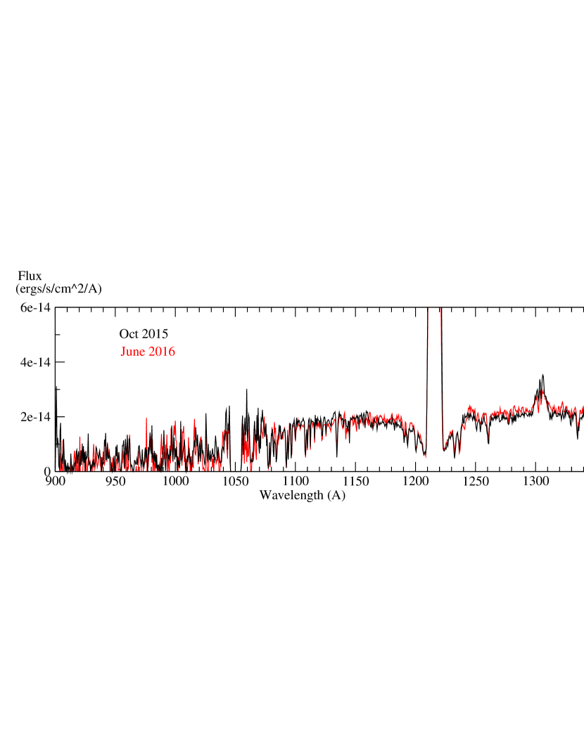
Figure 4b: The June 2016 HST/COS spectrum of T Pyxidis is shown (in red) together with the October 2015 spectrum (in black) and displays a slight increase in flux especially in the longer wavelengths.

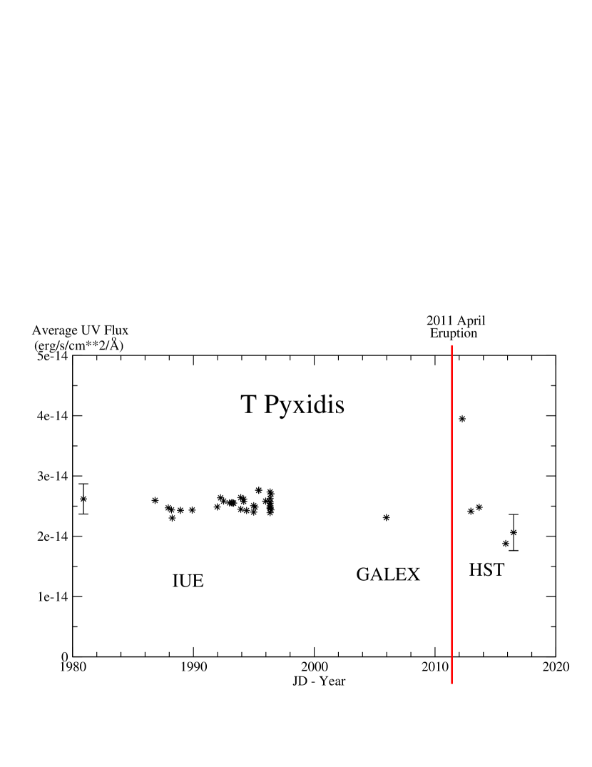
Figure 5: The average flux for the IUE SWP, GALEX and HST/STIS spectrum are shown as a function of time (see Tables 2 and 3 for exact dates). The flux was averaged over the spectral region $\sim 1400$ to $\sim 1700$ Å , excluding emission lines. For clarity the error bar (in $F_{\lambda}$) has been drawn only for the first and last data points and represents the average value of the flux error around 1400 Å (20 to 25%). IUE data points obtained over a period of a few days in 1996 reveal that the flux can vary by as much as $\sim 18$% ($\pm$9% from the median value). The 2005 GALEX and 2012-2013 HST data points appear within the flux fluctuation of the IUE pre-eruption data points. Only the 2015 and 2016 data, obtained more than $4\frac{1}{2}$ years after the eruption (vertical red line), show a drop below the pre-eruption level.

3 Modeling

Our spectral modeling tools and technique have been previously described extensively in numerous works such as Godon et al. (2012, 2016), as a consequence, we limit ourselves here to a brief description of the modeling but include a comprehensive account of the recent improvements we made over our previous UV spectral analysis of T Pyx in (Godon et al., 2014).

3.1 Modeling of the Accretion Disk Spectrum

For the disk we assume the standard model (Shakura & Sunyaev, 1973; Pringle, 1981), namely, the disk is optically thick, it has a negligible vertical thickness $H/r<<1$, it is axisymmetric and the energy dissipated between shearing adjacent annuli of matter is radiated locally in the $\pm$z directions. As a consequence, the temperature is solely a function of the radius $r$, and is completely defined by the mass $M_{\rm wd}$ of the central star, the mass accretion rate $\dot{M}$, and the inner radius of the disk $R_{\rm in}$. The luminosity and spectrum of the disk are obtained by integrating over the entire surface area of the disk from the inner radius $R_{\rm in}$ to the outer radius $R_{\rm out}$.

In order to generate a disk spectrum, we divide the disk into $N$ rings with radius $r_{i}(i,1,2..N)$ each with a temperature $T(r_{i})$ given by the standard disk model and defined when $M_{\rm wd}$, $\dot{M}$, and $R_{\rm in}$ are given. For each ring, a synthetic spectrum is generated by running Hubeny’s synthetic stellar atmosphere suite of codes TLUSTY, SYNSPEC and ROTIN (Hubeny, 1988; Hubeny & Lanz, 1995). A final disk spectrum is then obtained by running DISKSYN, which combines the rings spectra together for a given inclination and takes into account Keplerian broadening and limb darkening (Wade & Hubeny, 1998). TLUSTY & SYNSPEC are described in detail in Hubeny & Lanz (2017a, b, c).

Our present modeling includes a number of improvements we recently made as follows.

The Inner Disk Radius

The standard disk model, Wade & Hubeny (1998)’s disk models, and our previous disk models all assume that the inner radius of the disk corresponds to the radius of the central star $R_{\rm in}=R_{\rm wd}$. In other words, the radial thickness of the boundary layer is negligible: $\delta_{\rm BL}<<R_{\rm wd}$ (where the size of the boundary layer is determined by the vanishing of the shear $d\Omega/dR=0$ at $R_{\rm in}=R_{\rm wd}+\delta_{\rm BL}$ (Pringle, 1981), in cylindrical coordinates $(R,\phi,z)$). This assumption is valid for an optically thick boundary layer when the mass accretion rate is moderately large (here $\dot{M}\approx 10^{-9}-10^{-7}M_{\odot}$), and negligible in comparison to the Eddington limit ($\dot{M}<<\dot{M}_{\rm Edd}$). For a very large mass accretion rate, the size of the optically thick boundary layer increases (Godon, 1996, 1997) and one has $\delta_{\rm BL}\approx 0.1-0.5R_{\rm wd}$ or so. When the boundary layer is optically thin (which usually happens at low mass accretion rates), its size also increases (Narayan & Popham, 1993; Popham, 1999).

In the present work we take the inner radius of the accretion disk to be larger than the radius of the star ($R_{\rm in}>R_{\rm wd}$) to accommodate for the possible presence of an extended boundary layer. This also allows us to consider a heated WD with an inflated radius in comparison to the zero-temperature radius, or a disk that is truncated by the WD magnetic field. The important point here is that we do not generate a disk model with an inner radius at $R_{\rm wd}$ and truncate it at $R_{\rm in}$, but, rather, we generate a disk model with the inner radius at $R_{\rm in}>R_{\rm wd}$. Since the no-shear ($d\Omega/dR=0$) boundary condition is imposed at the disk inner radius (rather than the WD radius) this difference produces a disk that is colder in its inner region relatively to the standard disk model (it is a standard disk model with $R_{\rm wd}$ replaced by $R_{\rm in}>R_{\rm wd}$). Namely, the disk radial temperature profile (Pringle, 1981) can be written as

$$T_{\rm eff}(x)=T_{0}x^{-3/4}(1-x^{-1/2})^{1/4},$$ (1)

with

$$T_{0}=64,800~{}{\rm K}\times\left[\left(\frac{M_{\rm wd}}{M_{\odot}}\right)\left(\frac{\dot{M}}{10^{-9}M_{\odot}{\rm yr}^{-1}}\right)\left(\frac{R_{\rm in}}{10^{9}{\rm cm}}\right)^{-3}\right]^{1/4},$$ (2)

and where $x=R/R_{\rm in}$ (Wade & Hubeny, 1998), but now $R_{\rm in}$ is the inner radius of the disk (Godon et al., 2017b). The maximum disk temperature, $T_{\rm max}=0.488T_{0}$ reached at $x=1.36$, is given by

$$T_{\rm max}=177,826~{}{\rm K}\left(\frac{M_{\rm wd}}{M_{\odot}}\right)^{1/4}\left(\frac{\dot{M}}{10^{-6}M_{\odot}{\rm yr}^{-1}}\right)^{1/4}\left(\frac{R_{\rm in}}{10,000~{}{\rm km}}\right)^{-3/4},$$ (3)

where for convenience we have now written $\dot{M}$ in units of $10^{-6}M_{\odot}$yr^-1, which is the order of magnitude of the mass accretion we obtained for T Pyx in Godon et al. (2014). It is then apparent that for a $\sim 0.7M_{\odot}$ WD with a radius of $\sim 8,500$ km (see Section 1.2), one has $T_{\rm max}\approx 150,000$ K, while for a $\sim 1.35M_{\odot}$ WD with a radius of $\sim 2,000$ km, $T_{\rm max}\approx 500,000$ K.

We note, however, that the maximum disk temperature achieved in the inner region can be decreased by increasing $R_{\rm in}$. Our modified accretion disk models were already presented and used in Godon et al. (2017b) and Darnley et al. (2017), and further details can be found therein.

The Outer Disk Radius

In our previous work (Godon et al., 2014), based on the work of Wade & Hubeny (1998), the disk was extended to a radius where the temperature reached 10,000 K. Such a radius, depending on the binary separation, mass of the WD, mass accretion rate, and state of the system, could be larger or smaller than the actual radius of the disk. We improved our modeling by choosing the outer disk radius to represent the physical radius of the disk, which can now be extended to include outer rings with a temperature as low as 3,500 K.

Due to the tidal interaction of the secondary star, the size of the disk is expected to be between $0.3a$ (where $a$ is the binary separation) for a mass ratio $q=M_{2}/M_{1}\approx 1$, and about $0.6a$ for $q<<0.1$ (Paczynski, 1977; Goodman, 1993). T Pyx, with a binary mass ratio of $q=0.20\pm 0.03$ (Uthas et al. (2010), for a low inclination and a tidally limited disk radius), should have an outer disk radius $R_{\rm out}\approx 0.46a$ (based on the work of Goodman (1993)). However, some systems with a moderate mass ratio have exhibited a disk reaching all the way out to the limit of the Roche lobe radius, e.g. U Gem with a mass ratio $q=0.35$ and an expected disk radius of about $\approx 0.42a$ has been observed in quiescence to exhibit double peaked emission lines suggesting an outer disk radius of $0.61a$ (Echevarría et al., 2007). Consequently, in the present work we consider accretion disk models with a radius of $\approx 0.3a$ and $\approx 0.6a$.

The outer disk temperature, at $R=R_{\rm out}>>R_{\rm in}$, is given by

$$T_{\rm out}=T_{\rm eff}(x)\left|{}_{R=R_{\rm out}}=T_{0}x^{-3/4}\right|_{R=R_{\rm out}}=364,400~{}{\rm K}\left(\frac{M_{\rm wd}}{M_{\odot}}\right)^{1/4}\left(\frac{\dot{M}}{10^{-6}M_{\odot}{\rm yr}^{-1}}\right)^{1/4}\left(\frac{R_{\rm out}}{10,000~{}{\rm km}}\right)^{-3/4},$$ (4)

since $x>>1$. The outer disk temperature does not depend on the choice of the inner disk radius and, as expected, decreases with increasing $R_{\rm out}$. For $R_{\rm out}=360,000$ km ($\sim 0.6a$) we obtain $T_{\rm out}\approx 24,800$ K, and for a disk half this size ($\sim 0.3a$) we obtain $T_{\rm out}\approx 41,700$ K in the above equation.

Overall, for a given $M_{\rm wd}$ and $\dot{M}$, the inner disk temperature depends on the inner disk radius, and the outer disk temperature depends on the outer disk radius.

3.2 Dereddening

We updated our dereddening software and instead of using the IUERDAF task UNRED (based on Savage & Mathis (1979), and which we had been using for IUE data (Godon et al., 2014)), we generated our own script using the Fitzpatrick & Massa (2007) extinction curve (with $R=3.1$).

We combine the HST, GALEX, and IUE spectra and remove the unreliable spectral portions of GALEX and IUE (see Fig.2). The interstellar extinction produces a strong and broad absorption feature centered at 2175 Å(see Fig.6), due mainly to polycyclic aromatic hydrocarbons (PAH) grains (Li & Draine, 2001). We dereddened the spectrum for different values of $E(B-V)$, using the extinction curve from Fitzpatrick & Massa (2007). The absorption features vanishes for $E(B-V)=0.30$, and we therefore adopt this value of the reddening for T Pyx. From the visual inspection of the figure alone we infer an error of 0.05. An additional 20 percent error ($\pm 0.06$) has to be taken into account when using the 2175 Å bump (Fitzpatrick & Massa, 2007). It is worth mentioning, however, that PAHs, the dominant contributor to the 2175 Å bump, do not dominate the FUV extinction (Li & Draine, 2001), and three decades ago it was already shown that the 2175 Å bump correlates poorly with the FUV extinction (Greenberg & Chlewicki, 1983). This is further illustrated by the larger sample variance about the mean average Galactic extinction curve observed in the shorter wavelength of the FUV (Fitzpatrick & Massa, 2007). In the present work, we therefore adopt $E(B-V)=0.30\pm 0.08$, and refer the reader to Godon et al. (2014) (and to our conclusion section) for an investigation of how the assumed reddening affect our results, taking into account that in the literature the reddening toward T Pyx has been as low as 0.25 (Gilmozzi & Selvelli, 2007) and as large as 0.50 (Shore et al., 2013).

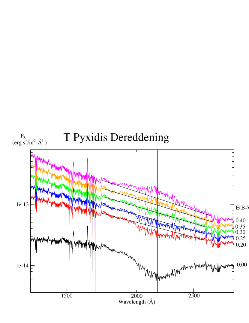
Figure 6: The combined HST STIS, GALEX, and IUE spectrum is presented here, where we have removed the unreliable spectral portions of GALEX and IUE (see Fig.2). The lower spectrum (solid black line) is the undereddened spectrum, namely $E(B-V)=0.00$ as indicated on the right. The interstellar extinction produces a strong and broad absorption feature centered at 2175 Å (marked with a vertical line). We dereddened the (bottom) spectrum for different values of $E(B-V)$ (again as indicated on the right), using the extinction curve from Fitzpatrick & Massa (2007). The absorption features vanishes for $E(B-V)=0.30$, and we therefore adopt this value of the reddening for T Pyx in the present work. In contrast, in our previous work (Godon et al., 2014) we obtained $E(B-V)=0.35$ using the Savage & Mathis (1979)’s extinction law.

3.3 Optical Wavelengths

In our current analysis we extend the wavelength coverage into the optical, thereby now generating disk and WD spectra from 900 Å to 7500 Å. Our UV-optical disk modeling has recently been applied in the spectral analysis of the most extreme RN M31N 2008-12a (Darnley et al., 2017).

T Pyx was observed by Williams (1983) in the optical in its pre-outburst state on Feb 1st, 1982, at UT 07:07 for 75 min, at the (MDM) McGraw-Hill Observatory with the 1.3 m telescope and a 2000 channel intensified Reticon spectrophotometer. An optical spectrum was obtained in the wavelength range 3500-7100 Å, thereby covering the Balmer jump. We digitally retrieved the T Pyx optical spectrum from Williams (1983) and scaled it to the pre-outburst (2008) optical spectrum obtained by Uthas et al. (2010), which is itself a flux-calibrated average of 200 spectra observed with the Magellan telescope (4000 Å to 5200 Å) . We use this spectrum to verify and validate our UV disk model and fit.

3.4 Parameter Space

In the present work we extend the modeling we carried out in Godon et al. (2014) over a slightly different region of the parameter space as follows. First we assume $E(B-V)=0.30$, while in Godon et al. (2014) we checked how the results vary for $E(B-V)=$0.25, 0.35, and 0.50. Similarly, we currently choose an inclination $i=20^{\circ}$ rather than assuming $i=10^{\circ}$ and $i=30^{\circ}$. We therefore expect the present results to “fall” between our previous results of $E(B-V)=0.25$ and $0.35$ and $i=10^{\circ}$ and $i=30^{\circ}$. However, in the present work we also check how the results are affected when assuming a large inclination, $i=60^{\circ}$, as suggested by Patterson et al. (2017). As in Godon et al. (2014) we run models for both $M_{\rm wd}=0.70M_{\odot}$ and $M_{\rm wd}=1.35M_{\odot}$. Due to size of the disk being limited between $\sim 0.3a$ and $\sim 0.6a$, we obtain outer disk temperatures of order $\sim 40,000$ K and $\sim 20,000$ K, respectively, while in our previous work the disk extended to a radius where $T\sim 10,000$ K. We choose (as explained earlier) the inner radius of the disk to be larger than the WD radius.

Because the Gaia DR2 data (Prusti et al., 2016; Brown et al., 2018; Eyer et al., 2018) was released after the manuscript had been submitted and reviewed (and just before it was re-submitted), we include models for the Gaia distance of (see section 1.2) $d=3.3^{+0.5}_{-0.4}$kpc in the end of the Results and Discussion Sections.

4 Results

As in Godon et al. (2014), in the following we model the co-added post-outburst HST Dec 2012 and Jul 2013 spectrum, combined with the pre-outburst co-added IUE spectra, GALEX spectrum (as shown in Fig.6), together with the pre-outburst optical spectrum. The Oct 2015 and Jun 2016 HST spectra exhibit a small drop ($\sim 20$%) in flux in comparison to the Dec 2012 and Jul 2013 HST spectra, but are otherwise almost identical to them. The mass accretion rate corresponding to the Dec 2012 and Jul 2013 spectra can then simply be derived by scaling our derived mass accretion rate.

Since the actual mass accretion rate is not known a priori, it has to be found by decreasing or increasing $\dot{M}$ until a fit at a the distance of 4.8 kpc is found. If the decrease or increase in $\dot{M}$ is of the order of $\sim 40$% or smaller ($\Delta\dot{M}/\dot{M}<0.4$), then it is carried out by linear scaling the flux of the disk model; if it is larger than that ($\Delta\dot{M}/\dot{M}>0.4$), then a new disk model is generated. Also, some of the parameters that are varied do not provide a noticeable change in the results and, consequently, we only list the disk models exhibiting noticeable changes. As the mass accretion rate considered here is extremely large, the contribution of the WD to the spectrum is completely negligible and, consequently, cannot be modeled. Therefore, we present here only a limited number of models.

We first started with a $1.35M_{\odot}$ WD with a radius of 2,000 km, and a corresponding binary separation $a\approx 600,000$ km. Since the mass accretion rate needed to scale to the distance is very large (of the order of $10^{-6}M_{\odot}$yr^-1) we set the inner radius of the disk $R_{\rm in}$ to $1.1R_{\rm wd}$, $1.2R_{\rm wd}$, and $1.5R_{\rm wd}$, to mimic a geometrically thick boundary layer. These models gave identical results and we decided to adopt $R_{\rm in}=1.1R_{\rm wd}$. We first checked the results for an outer disk radius of the order of $0.3a$ (limited by tidal interaction), which, due to the discrete values of the disk’s rings in the model, gave $R_{\rm out}=0.27a$. For this model, model #1 in Table 4, we obtained a mass accretion rate $\dot{M}=1.2\times 10^{-6}M_{\odot}$yr^-1 with a minimum disk temperature at $R_{\rm out}$ of $T_{\rm disk}^{\rm out}=46,700$ K. This model is presented in Fig.7 and fits the UV data relatively well up to a wavelength $\lambda\approx 2,000$ Å. At longer wavelengths the model becomes too steep and the spectral slope of the data becomes flatter with increasing wavelength. Namely, the continuum slope in the optical is flatter than the NUV continuum slope, which itself is flatter than the FUV continuum slope. The disk model does not show any sign of the Balmer jump because the disk has a temperature $T>45,000$ K. The observed optical spectrum does not clearly show the Balmer jump in absorption nor in emission, but does show hydrogen emission lines as well as some absorption lines.

Next, we increased the disk size to a maximum value of $\approx 0.6a$ (about the size of the Roche lobe radius), which, again due to the discrete values of the disk rings, gave $R_{\rm out}=0.59a$. Since this disk surface area is larger, it requires a smaller mass accretion rate to scale to a distance of 4.8 kpc. For this model, model #2 in Table 4, we obtained $\dot{M}=5.6\times 10^{-7}M_{\odot}$yr^-1 with a minimum disk temperature of $T_{\rm disk}^{\rm out}=23,500$ K at $R_{\rm out}$. This model, shown in Fig.8, exhibits a smaller discrepancy in the optical wavelengths and starts to show a “semblance” of Balmer jump which is not particularly in disagreement with the optical spectrum itself. Altogether, the larger disk model (#2) provides an overall better fit than the smaller disk model (#1).

We then checked the effect of a higher inclination on the results. We increased the inclination from $i=20^{\circ}$ to $i=60^{\circ}$ in model #2 which decreases the overall flux by about a factor of two. Consequently, for this new model, model #3 in Table 4, we had to increase the mass accretion rate to $1.36\times 10^{-6}M_{\odot}$yr^-1 to obtain the correct fit to the distance. This model exhibits wider and shallower absorption lines, but as the observed spectrum exhibits mainly emission lines, the fit is carried out on the continuum. This model fit is similar to models #1 and #2 in the UV; in the optical, however, the model is not as good as model #2, but it is better than model #1. For all the disk models considered here, we found that the increase in the inclination (to $i=60^{\circ}$) reduces the flux level by a factor of $\sim 2$ (and therefore increasing the mass accretion rate by the same factor), due mainly to the reduced projected emitting area and somewhat to the coefficient of the limb darkening. For clarity we only list model #3 in Table 4.

Table 4: T Pyxidis Disk Models Parameters

Model	$M_{\rm wd}$	$R_{\rm wd}$	$a$	$R_{\rm in}$	$R_{\rm out}$	$\dot{M}$	$T_{\rm disk}^{\rm out}$	$i$	d	$\Delta M$
Number	$(M_{\odot})$	($10^{3}$km)	$(10^{5}{\rm km})$	$(R_{\rm wd})$	$(a)$	$(10^{-X}M_{\odot}$yr${}^{-1})$	(103K)	(deg)	(kpc)	($10^{-X}M_{\odot}$)
-19	1.35	2.0	6.0	1.1	0.27	1.20(-6)	46.7	20	4.8	5.28(-5)
-18	1.35	2.0	6.0	1.1	0.59	5.60(-7)	23.5	20	4.8	2.46(-5)
-17	1.35	2.0	6.0	1.1	0.59	1.36(-6)	26.7	60	4.8	5.98(-5)
-16	0.70	8.5	5.0	1.1	0.30	1.92(-6)	40.0	20	4.8	8.45(-5)
-15	0.70	8.5	5.0	1.1	0.61	1.24(-6)	24.2	20	4.8	5.46(-5)
-14	0.70	8.5	5.0	1.5	0.30	2.15(-6)	40.7	20	4.8	9.46(-5)
-13	0.70	8.5	5.0	1.5	0.59	1.36(-6)	26.0	20	4.8	5.99(-5)
-12	1.35	2.0	6.0	7.0	0.59	7.90(-7)	25.7	20	4.8	3.48(-5)
-11	1.35	2.0	6.0	1.0	0.30	1.03(-7)	24.6	20	2.9	4.53(-6)
-10	1.35	2.0	6.0	1.0	0.30	1.34(-7)	24.6	20	3.3	5.90(-6)
-9	1.35	2.0	6.0	1.0	0.30	1.76(-7)	24.6	20	3.8	7.74(-6)
-8	1.35	2.0	6.0	1.0	0.60	9.00(-8)	14.8	20	2.9	3.96(-6)
-7	1.35	2.0	6.0	1.0	0.60	1.15(-7)	14.8	20	3.3	5.06(-6)
-6	1.35	2.0	6.0	1.0	0.60	1.53(-7)	14.8	20	3.8	6.73(-6)
-5	0.70	8.5	5.0	1.1	0.30	6.80(-7)	40.0	20	2.9	2.99(-5)
-4	0.70	8.5	5.0	1.1	0.30	8.70(-7)	40.0	20	3.3	3.83(-5)
-3	0.70	8.5	5.0	1.1	0.30	1.15(-6)	40.0	20	3.8	5.06(-5)
-2	0.70	8.5	5.0	1.1	0.60	4.21(-7)	24.2	20	2.9	1.85(-5)
-1	0.70	8.5	5.0	1.1	0.60	5.45(-7)	24.2	20	3.3	2.40(-5)
0	0.70	8.5	5.0	1.1	0.60	7.22(-7)	24.2	20	3.8	3.18(-5)

Note. — In column 4 we list the binary separation $a$, followed by the inner and outer radii of the disk $R_{\rm in}$ and $R_{\rm out}$ respectively in columns 5 and 6. The outer disk temperature $T_{\rm disk}^{\rm out}$ (reached at $R=R_{\rm out}$) is given in column 8 (it is the lowest temperature in the disk). Models 9 through 20 were computed after completion of the manuscript to check effect of the just-released Gaia distance of $3.3^{+0.5}_{-0.4}$kpc. The negative number in parenthesis in columns (7) and (11) denotes the exponent “X” in the unit row. The last column indicates the mass of the accreted envelope over 44 years.

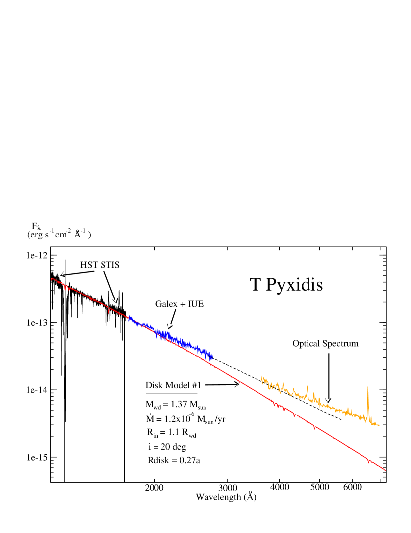
Figure 7: The HST STIS, GALEX, IUE and optical spectra of T Pyx are presented here (color coded) on a log-log scale together with accretion disk model # 1 (Table 4; solid red line). The observed spectra have been dereddened assuming $E(B-V)=0.30$. The optical spectrum is in orange. The slope of the disk model departs from the data at wavelengths $>2,000$ Å, namely the slope of the GALEX+IUE spectrum (in blue) is flatter than the slope of the STIS spectrum (in black), and the optical spectrum itself is even flatter (as shown by the dashed black line for comparison). The disk model does not show the Balmer jump because the disk everywhere has a temperature $T>45,000$ K.

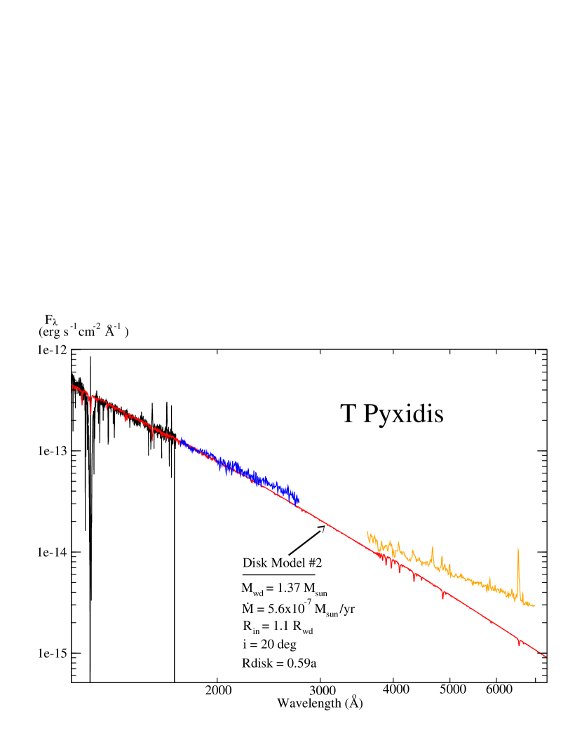
Figure 8: Same as in Fig.7, but now the disk has been allowed to extend to the Roche lobe radius, $\approx 0.6a$, where $a$ is the binary separation (model # 2 in Table 4). Since the disk radius is larger, it has a a larger flux at the same accretion rate and the resulting $\dot{M}$ needed to fit the data is lower than in model # 1 (Fig.7). The outer disk reaches a temperature as low as 23,500 K and helps flatten the slope of the theoretical spectrum resulting in a slightly higher flux in the optical range than model # 1. Because of its lower temperature, the disk model exhibits a Balmer jump, which is very weak.

We continued by running models with a lower WD mass, $0.7M_{\odot}$, agreeing with the analysis of Uthas et al. (2010), and adopted a WD radius of 8,500 km, corresponding to a temperature of $\sim$30,000 K for such a WD mass (Woods, 1995). For this primary mass, the binary separation shrinks to $\sim$500,000 km. We chose an inner disk radius $R_{\rm in}=1.1R_{\rm wd}$ and obtained a mass accretion rate of $\dot{M}=1.92\times 10^{-6}M_{\odot}$yr^-1 and $\dot{M}=1.24\times 10^{-6}M_{\odot}$yr^-1 for an outer disk radius of $0.30a$ (model #4) and $0.61a$ (model #5) respectively. These two models gave the same fits as for the larger WD mass models #1 and #2 and are indistinguishable from them: model #5 fits the optical region better than model #4 and presents an identical fit as model #2 shown in Fig.8. The reason for the similarity of the models lies in the fact that the region of the disk contributing to the UV has about the same temperature, as shown in Table 4 by the outer disk temperature reached at $R_{\rm out}$ for models #4 and #5. The very inner disk is colder in the $0.7M_{\odot}$ models than in the $1.35M_{\odot}$ models and choosing a slightly larger inner disk radius, $R_{\rm in}=1.5R_{\rm wd}$ increases the mass accretion rate by about 10% as shown in Table 4 for models #6 and #7. The fits are, however, identical and one cannot differentiate between the $1.1R_{\rm wd}$ and $1.5R_{\rm wd}$ models.

As stated earlier, the just-released Gaia parallax gives a distance of $3.3^{+0.5}_{0.4}$kpc, significantly smaller than the $4.8-5.0$ kpc of Sokoloski et al. (2013); De Gennaro Aquino et al. (2014), thereby demanding further model fits. We, therefore, carried out post facto 12 more model fits: for $M_{\rm wd}=1.35M_{\odot}$ and $M_{\rm wd}=0.70M_{\odot}$, each for a disk outer radius $R_{d}=0.3a$ and $R_{d}=0.6a$, and for a distance of $d=$2.9, 3.3, and 3.8 kpc. These 12 models are listed in Table 4 (number #9 through # 20). Overal the Gaia distance gives a mass accretion of the order of $10^{-7}M_{\odot}$yr^-1 for $M_{\rm wd}=1.35M_{\odot}$ and $5-7\times 10^{-7}M_{\odot}$yr^-1 for $M_{\rm wd}=0.70M_{\odot}$. In the UV range these 12 models provide a fit to the flux continuum slope as good as models 1 & 2 in Figs.7 & 8. Our ex post facto results for the Gaia distance are discussed in the next section.

5 Discussion

Our current results agree with our previous analysis (Godon et al., 2014) that, during its quiescent state, T Pyx has a mass accretion rate $\dot{M}$ of the order of $10^{-6}M_{\odot}$yr^-1 for a distance of $4.8$ kpc. This is about 10 times larger than the estimate from Patterson et al. (2017), who derived the mass accretion rate from the period change of the system both in quiescence and as a result of the eruption. The discrepancy between our results and Patterson et al. (2017)’s vanishes when we considered the Gaia derived distance of $3.3$ kpc and a WD mass of $1.35M_{\odot}$. However, the discrepancy remains for the low WD mass ($0.7M_{\odot}$) assumption.

The exact value of $\dot{M}$ we obtain here depends on the assumed WD mass, inclination, reddening, outer disk radius and distance to the system. We discuss these here below.

The Optical Range

An important improvement is the inclusion of the optical data, which reveal that the optical continuum slope is flatter than the NUV continuum slope, which itself is flatter than the FUV continuum slope (see Figs.7 and 8). This is contrary to the analysis of Gilmozzi & Selvelli (2007) who claimed that the slope becomes steeper at longer wavelengths. The discrepancy is likely due to the limited number of data points used by Gilmozzi & Selvelli (2007). The slope of the optical continuum is compatible with an $\sim$8,000 K stellar atmosphere, but it does not reveal the Balmer jump (contrary to a stellar atmosphere spectrum). Also the emitting area of a 8,000 K component would have to be larger than the size of binary system to produce such a flux at such a low temperature. It is, therefore, clear that a significant contribution to the optical flux comes from the optically thick accretion disk.

We further present model #1 and #2 together with the optical data in Fig.9 on a linear scale. We display the optical spectrum from Williams (1983) together with the optical spectrum from Uthas et al. (2010) to which it was scaled. The similarity between the emission lines and slope of the continuum between the two optical spectra provides further evidence that the system remains in a state relatively similar over many years, as already demonstrated by the UV spectra shown in Fig.3. The discrepancy between model #2 and the optical data is only $\sim 2\times 10^{-15}$erg s^-1cm^-2Å^-1, and the difference between model #1 and model #2 is of the same order. This is rather small when compared to the UV flux which is 10 to 100 times larger, because the disk emits only a tiny fraction of its energy in the optical band. The ex post facto models based on the Gaia distance are very similar to model 1 & 2, except for models #12, 13 and 14, which have a large disk radius ($0.6a$) and a (relatively) lower mass accretion rate ($\sim 10^{-7}M_{\odot}$yr^-1). These 3 models have an outer disk temperature reaching $\sim 15,000$ K and exhibit a strong Balmer jump, unlike the optical spectrum. Model #13 is shown in Fig.9 for comparison. This indicates that the radius of the disk is probably closer to $0.3a$ than to $0.6a$. The discrepancy in the optical is not inconsistent with the data, as this possibly indicates that an additional component contributing flux in the longer wavelengths is missing from our modeling. Similar results were obtained in the spectral modeling of the RN M31N 2008-12a (Darnley et al., 2017) . Since we rule out an 8,000 K component as the source of the optical flux, the secondary cannot possibly contribute much to the optical, unless its irradiation by the inner disk increases its temperature significantly. We also note that the optical emission from the nebula (extended shell) is rather negligible with a continuum flux level of $\sim 10^{-17}$erg^-1s^-1Å^-1 (Williams, 1982), two orders of magnitude smaller than the continuum flux level of the optical spectra.

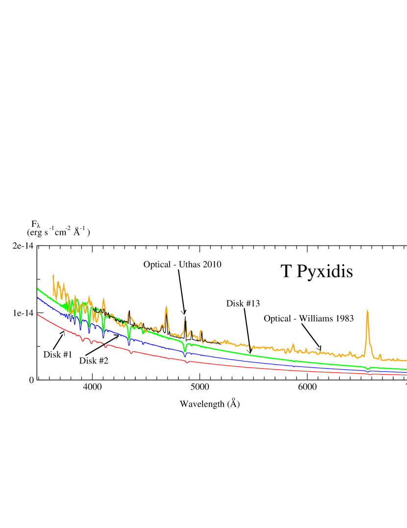
Figure 9: Models #1 (with an outer disk radius of $0.27a$, in blue) and #2 (with an outer disk radius of $0.59a$, in red) are shown on a linear scale together with the optical spectrum of Williams (1983) (in orange). The optical spectrum of Williams (1983) was scaled to fit the optical spectrum obtained by Uthas et al. (2010) (in black). The discrepancy between model #2 and the optical spectrum could be attributed to an accretion disk wind (Matthews et al., 2015) which would appear here to have a continuum flux contribution of about $2\times 10^{-15}$erg s^-1cm^-2Å^-1. The models based the 3.3 kpc Gaia distance give very similar results except for models #12, 13 and 14 which have a colder outer disk displaying a strong Balmer jump. Model # 13 is shown for comparison.

Accretion Disk Wind Contribution

While the best accretion disk models seem to fit the observed spectra down to about 2000 Å, the models become too blue in the longer wavelengths of IUE and in the optical. Often, CV disk-dominated systems have spectra that cannot be fitted with standard disk models, the models are too blue both in the UV (Puebla et al., 2007) and in the optical (Matthews et al., 2015). It was suggested (Matthews et al., 2015) that an accretion disk wind might be responsible for providing a continuum flux in addition to the contribution from the optically thick disk, making the observed overall spectrum redder than that from an optically thick disk model. The disk wind is also believed to be responsible for the formation of the observed sharp emission lines and for the absence of the Balmer jump when this latter is expected to be in absorption in the spectra of disk-dominated CVs. It is possible that the discrepancy between our optically thick disk model and the observed spectra is due in part to the lack of an accretion disk wind in our modeling. In the present case, however, the truncation of the outer disk model together with the high mass accretion rate generate a theoretical spectrum that does not exhibit a Balmer jump in agreement with the observed optical spectrum.

Long-term behavior

T Pyx seems to have faded by 2 mag since the 1866 nova eruption (Schaefer, 2005; Schaefer et al., 2010), and a look at its AAVSO light curve does indicate a slight decrease in the $\sim$25 years preceding the 2011 eruption (Fig.1). The light curve displaying the decline from the 2011 eruption shows that the system is still possibly declining, as its magnitude is still increasing. This is further reinforced by our UV light curve (Fig.5). In addition, it appears that both the optical (AAVSO) and UV light curves exhibit a drop of the quiescent magnitude/flux across the 2011 eruption: the quiescent magnitude/flux reached after the 2011 eruption (say in 2016) is lower than its pre-outburst value. This shows that the mass accretion rate in T Pyx is not only declining gradually, but it is also declining after each outburst (or at least after the last outburst), namely in “steps”. At the present time, this step consists in a 20 percent drop in the mass accretion rate (Fig.5).

X-ray Observations

We have used here optical data to help impose constraints on the spectral analysis, and, as in Godon et al. (2017b), we now wish to use X-ray data to further constrain and interpret the results of the spectral analysis. The main characteristics of the X-ray observations of T Pyx obtained during quiescence (Balman, 2010) is the fact that the X-ray luminosity is orders of magnitude smaller than the expected disk luminosity and that it originates in the shocked nebular material rather than in the inner accretion disk or boundary layer.

In the case of a massive WD ($1.35M_{\odot}$) accreting at a rate of the order of $10^{-6}M_{\odot}$yr^-1 (models #1, 2, & 3), the temperature in the inner disk (even without a boundary layer) reaches a maximum of $\sim$500,000 K, and drops to $\sim$350,000 K for $\dot{M}\approx 10^{-7}M_{\odot}$yr^-1. Such a high temperature component is expected to show in the soft X-ray band,and the boundary layer temperature would possibly be of the same order of magnitude. However, X-ray observations of T Pyx (Greiner & Di Stefano, 2002; Selvelli et al., 2008; Balman, 2010) do not provide supporting observational evidence for such an X-ray source scenario.

In contrast, if we consider the $0.7M_{\odot}$ WD mass disk models, the resulting maximum temperature in the inner disk reaches $\sim$170,000 K at $R=1.36R_{\rm in}$, dropping to $\sim$150,000 K at $R=2.10R_{\rm in}$, and $\sim$100,000 K at $R=4.00R_{\rm in}$. This is for $R_{\rm in}=1.1R_{\rm wd}$ (models # 4 & 5), and the temperature drops an additional 20 percent for $R_{\rm in}=1.5R_{\rm wd}$ (models # 6 & 7). A slightly lower temperature is reached for models #15 thru #20. As such the disk should emit in the EUV rather than soft X-ray, with the inner disk peaking around 300 Å. The optically thick boundary layer itself could be geometrically thick (even if it is dynamically thin, (Godon et al., 1995)), with a similar temperature ($\sim 10^{5}$ K). Such a scenario would explain the low X-ray luminosity as all the energy would be radiated in the EUV. Many CVs accreting at a high mass accretion rate have similar X-ray characteristics, namely no sign of an optically thick boundary layer (Ferland et al., 1982), but instead a very faint hard X-ray emission with a luminosity orders of magnitude smaller than the disk luminosity (Mauche et al., 1995; van Teeseling et al., 1996; Baskill et al., 2005). The consequence of having a strong EUV source is that the radiation is expected to interact strongly with the ISM and hence the EUV luminosity is greatly reduced. EUV sources are mostly detectable out to a distance of only a few hundred parsecs and at the shortest wavelengths (Barstow, 2014).

Therefore, one option is that the mass of the WD is $0.7M_{\odot}$ (Uthas et al., 2010), and that the accretion disk emits mostly in the EUV, and that the EUV radiation cannot reach us. The problem with this scenario is that the X-ray emission during outburst argues against a low mass WD, and a $0.7M_{\odot}$ WD accreting at a high rate grows to large radii with no outburst (Newsham et al., 2014).

We note, however, that in order for a $1.35M_{\odot}$ WD accreting at a high rate ($\sim 10^{-7}-10^{-6}M_{\odot}$yr^-1) to not exhibit X-ray emission, the inner radius of the disk has to be much larger than the anticipated WD radius (see equation 3). In Table 4 we list such a model, # 8. In that model, we increased the inner disk radius till the maximum temperature in the inner disk drops to 150,000 K. For this to happen we find a radius of $\sim$14,000 km, namely 7 times larger than the expected WD radius (2,000 km for a $1.35M_{\odot}$). For an outer disk radius of 0.59a, the disk gives a mass accretion rate of $7.9\times 10^{-7}M_{\odot}$yr^-1. The fit is as good as model # 2. Similarly, if we consider model # 13 (similar to model #8 but adjusted to the Gaia distance), we find that in order to reduce the inner disk temperature from 350,000 K to 150,000 K, we need to increase the inner disk radius to 8,000 km, namely 4 times larger than the expected WD radius. However, we find no physical explanation for the inner disk radius to be so large (T Pyx is not an intermediate polar and we do not consider disks departing from the standard model).

Accreted Mass versus Ejected Mass

We recapitulate our results in Figs.10a, b, & c, where we compare the accreted envelope mass obtained from our analysis with the estimates of the ejected envelope mass from the literature. Our previous accreted mass estimate for $E(B-V)=0.25$, 0.35 and 0.50 (all in black) were computed in Godon et al. (2014) for $i=10^{\circ}$ and $30^{\circ}$. Our new results investigating the effects of the size of the disk for $E(B-V)=0.30$ and $i=20^{\circ}$ are in red, and as expected fall between our previous $E(B-V)=0.25$ and $E(B-V)=0.35$ results. The ensuing accreted envelope is more massive when assuming a smaller disk radius. Our new results investigating the effects of a large inclination are in blue and indicate that the accreted envelope mass increases by a factor of two when increasing the assumed inclination from $20^{\circ}$ to $60^{\circ}$. These results confirm that if we assume a distance of 4.8 kpc for most of the parameter space the accreted envelope is larger than the ejected one and the WD should increase its mass with time.

Howevere, if the WD mass in T Pyx is massive and if the distance to the system is $\sim 3.3$ kpc, then T Pyx is losing more mass than it is accreting.

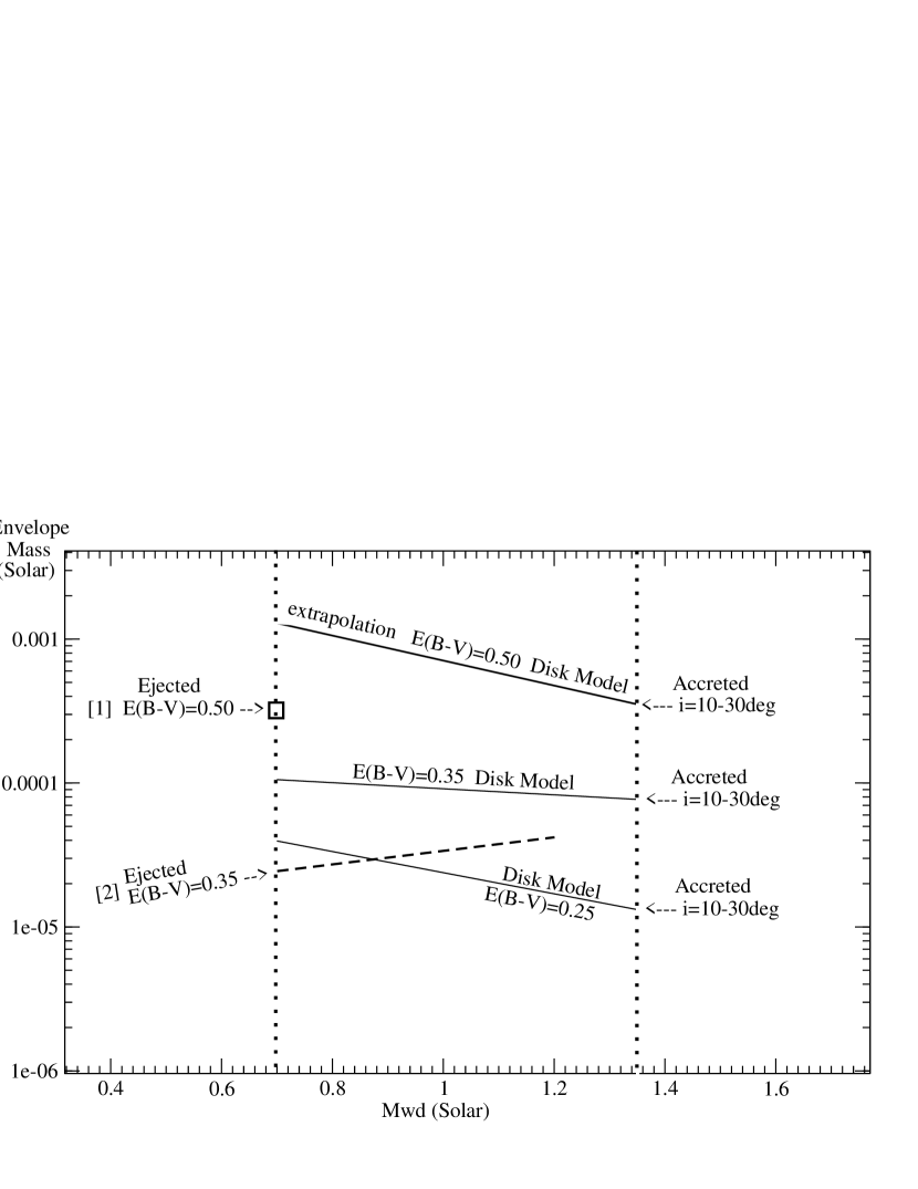
Figure 10a: The ejected and accreted envelope masses (Y-axis, in units of Log($M_{\odot}$); per nova eruption) as a function of the assumed WD mass (X-axis, in units $M_{\odot}$), based on the 2011 eruption and modeling of the quiescent spectra. The assumed $0.7M_{\odot}$ and $1.35M_{\odot}$ WD masses are indicated with the vertical dotted lines. The three solid black lines are the accreted envelope mass estimates from the UV spectral modeling we carried out in Godon et al. (2014) assuming different values for the reddening and for a system inclination of $10^{\circ}$ and $30^{\circ}$ (as marked on the figure). The first ejected envelope mass [1] (black square symbol in the upper left) is the mass loss maximum estimate of Nelson et al. (2014) assuming a reddening of $E(B-V)=0.50$ (Shore et al., 2013) and $M_{\rm wd}=0.7M_{\odot}$. This ejected mass is to be compared to our accreted envelope mass for the same reddening (the upper solid black line) and same WD mass. The second ejected envelope mass [2] (dashed black line) is from Patterson et al. (2017) and was computed assuming $E(B-V)=0.35$ for a range of WD masses. This ejected mass estimate is to be compared to our accreted envelope mass with the same reddening, namely the (almost horizontal) solid black line in the middle of the graph. Our estimate of the accreted envelope mass for a low reddening $E(B-V)=0.25$ (as derived by Gilmozzi & Selvelli (2007)) is the lower solid black line. Our previous results (assuming $d=4.8$ kpc) indicate that the accreted mass is larger than the ejected mass and the WD mass is possibly growing with time.

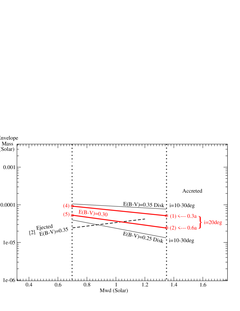
Figure 10b: The ejected and accreted envelope masses as a function of the WD mass as in Fig.10a. We have now added our new results assuming a distance of 4.8 kpc (two thick red lines), using a system inclination of $20^{\circ}$ and dereddening the spectra for $E(B-V)=0.30$. The models from Table 4 are indicated with an asterisk * and their respective number (1), (2), (4), and (5) and the thick solid red lines show the interpolation between the $0.7M_{\odot}$ and $1.35M_{\odot}$ models. For a disk tidally truncated at $0.3a$ (upper thick red line) the accreted mass envelope will be larger than for disk extending all the way to the Roche lobe ($0.6a$, lower thick red line). Consistent with our previous results, the present $E(B-V)=0.30$ results (the two thick red lines) fall between our $E(B-V)=0.25$ and 0.35 models (the two thin black lines). For clarity we have removed the $E(B-V)=0.50$ ejected and accreted mass envelopes from this graph.

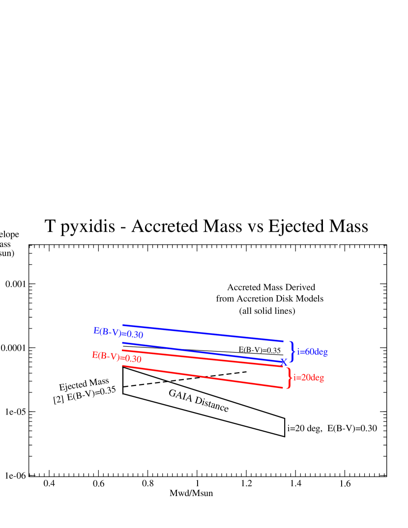
Figure 10c: The ejected and accreted envelope masses as a function of the WD mass as in Fig.10b. We have now added two thick solid blue lines for a system inclination of $60^{\circ}$ (as marked on the right). Model # 3 from Table 4 is marked with a large “X” sign. For clarity we have not marked models # 6 and 7 and we have removed the vertical dotted lines delimiting the WD masses $0.7M_{\odot}$ and $1.35M_{\odot}$. Increasing the inclination from 20^∘ (in red) to 60^∘ (in blue) results in an accreted envelope mass twice as large. The results presented in Figs. 10a, b, and c, were all obtained assuming a distance of 4.8 kpc. Our ex post facto results taking into account the shorter Gaia distance of $3.3^{+0.5}_{-0.4}$ kpc have been marked with the thick black line parallelogram in the lower part of the graph as the closer distance reduces the mass accretion rate.

6 Summary and Conclusion

We have carried out a UV and optical spectral analysis of recent HST observations of T Pyx in its quiescent and late declining states with an improved version of our accretion disk models. Using archival IUE data, optical data and results from X-ray observations, we show that the results heavily depends on the assumed parameters. We summarize our findings as follows.

1. Both the optical data (as of late 2017) and the UV data (as of mid-2016) indicate that T Pyx is still declining from its 2011 outburst.

2. Both the UV and optical data show that during the pre-outburst quiescent phase the system was in a relatively steady state with the same continuum shape exhibiting a fluctuation of only 9% in the continuum flux level, which can possibly be attributed to orbital modulation.

3. The UV clearly reveals a drop in the accretion rate across the outburst, namely when comparing the pre-outburst spectra to the late decline post-outburst spectra. This drop is confirmed by the AAVSO light curve (Fig.1), which also exhibits a drop across the outburst. We suggest that the system possibly experiences such a drop, after each recurring nova eruption, which might contribute to the 2 mag fading since 1866.

4. The previously accepted distance of $4.8$ kpc gives a large mass accretion rate ($\dot{M}\approx 10^{-6}M_{\odot}$yr^-1, ten times larger than the estimate of Patterson et al. (2017)) yielding to an accumulated envelope mass of $\approx 2.5-9.5\times 10^{-5}M_{\odot}$ (models 1-8). The mass ejected during the eruption is estimated to be $\sim 3\times 10^{-5}M_{\odot}$ (Patterson et al., 2017). This would imply that the T Pyx WD mass increased from 1966 (post-outburst) to 2011 (post-outburst), in agreement with Newsham et al. (2014) who predict that, irrespective of the actual mass of the WD, the WD will continue to grow in mass. However, the latest distance estimate from Gaia ($\sim 3.3$ kpc), gives an accumulated envelope mass as low as $\approx 4-8\times 10^{-6}M_{\odot}$ (models 9-14). Only if the WD in T Pyx is as low as $0.7M_{\odot}$ does the accumulated envelope mass reaches $\approx 2-5\times 10^{-5}M_{\odot}$ (models 15-20).

5. Our results indicate that if the T Pyx’s inclination is large, then the mass accretion rate must be larger by at least a factor of two. A larger inclination might, as a result of an inflated disk self-obscuration, explain why no soft X-ray emission is observed from the inner disk and how the UV flux varies by $\pm$9%. In this case the system would emit soft X-rays but it wouldn’t be observed.

6. If, however, the system is not emitting any soft X-rays at all, it is possible that the WD mass might be as small as $0.7M_{\odot}$ (Uthas et al. (2010), in disagreement with the theory Starrfield et al. (1985); Newsham et al. (2014)), with an inflated radius, and the disk inner radius might be $R_{\rm in}\approx 1.5R_{\rm wd}$ to explain the low inner disk/boundary layer temperature emitting in the EUV rather than in the soft X-ray band. Such EUV radiation would be absorbed by the ISM and would not be observable at a distance of 4.8 kpc. For a $1.35M_{\odot}$ WD accreting at a high rate to peak in the EUV (rather than in the X-ray) band, the inner radius of the disk would have to be 4-7 times larger than the actual radius of the $1.35M_{\odot}$ WD.

7. The reddening toward T Pyx remains largely unknown. A lower value of $E(B-V)\approx 0.25-0.35$ is obtained when using the 2175 Å PAH bump, which correlates poorly with the FUV extinction, (Greenberg & Chlewicki, 1983). A value twice as large, $E(B-V)\approx 0.50$, is obtained using the diffuse interstellar bands, however, $E(B-V)$ versus the $W_{\lambda}$(5780.5) has a rather large scatter when considering the data points individually (Friedman et al., 2011). Both techniques have their limitations and the results have to be considered for all values $E(B-V)=0.35^{+0.15}_{-0.10}$ (Fig.10).

To conclude, we point out two possible scenarios emerging from our analysis as follows.

(i) The WD is massive, $1.35M_{\odot}$, with a small radius, and due to the high accretion rate the inner disk emits soft X-rays which are blocked by the thick portion of the disk possibly viewed at a large inclination $i=60^{\circ}$. There is no restriction on the reddening.

(ii) The inner radius of the disk is large ($\sim 10-15,000$ km, due to either a small WD mass $0.70M_{\odot}$, or the truncation of the inner disk), the inclination is $20\pm 10^{\circ}$, and the reddening is probably $E(B-V)\approx 0.25-0.30$ (to keep $\dot{M}$ to a value of $\sim 10^{-6}M_{\odot}$yr^-1). The inner disk and boundary layer have a maximum temperature $\sim 150,000$ K peaking in the EUV. At a distance of a few kpc the EUV radiation is absorbed by the ISM.

In both cases the disk is large, and the UV light is modulated by the orbital motion as matter from the L1-stream overflow the disk rim and further masks parts of the inner disk. Most importantly, the newly derived distance from the Gaia DR2 data, for the most plausible values of the WD mass ($1.35M_{\odot}$) and reddening ($\approx 0.3$), imply a mass accretion rate of the order of $10^{-7}M_{\odot}$yr^-1, such that the accumulated envelope mass is actually smaller than the mass ejected during the eruption, indicating that the WD mass does not grow in mass. However, the Gaia distances for variable/binary stars have to be taken with some reservations (Eyer et al., 2018).

References

- Balman (2010) Balman, S. 2010, MNRAS, 404, L26
- Barstow (2014) Barstow, M.A., Casewell, S.L., Holberg, J.B., & Kowalski, M.P. 2014, Advances in Space Research, 53, 1003
- Baskill et al. (2005) Baskill, D.S., Wheatley, P.J., Osborne, J.P. 2005, MNRAS, 357, 626
- Bessel (2005) Bessel, M.S. 2005, ARA&A, 43 293
- Bowyer et al. (1994) Bowyer, S., Lieu, R., Lampton, M., Lewis, J., Wu, X., Drake, J.J., and Malina, R.F. 1994, ApJS, 93, 569
- Bowyer et al. (1996) Bowyer, S., Lampton, M., Lewis, J., Wu, X., Jelinsky, P., and Malina, R.F. 1996, ApJS, 102, 129
- Brown et al. (2018) Brown, A.G.A., Vallenari, T., Prusti, J.H.J., de Bruijne, et al. 2018, A&A, in press
- Collins (1992a) Collins, P. 1992a, IAU Circ., No.5454
- Collins (1992b) Collins, P. 1992b, AAVSO Circ., No.257
- Darnley et al. (2017) Darnley, M.J., Hounsell, R., Godon, P. et al. 2017, ApJ, 850, 146
- De Gennaro Aquino et al. (2014) De Gennaro Aquino, I., Shore, S.N., Schwartz, G.J., Mason, E., Starrfield, S., and Sion, E.M. 2014, A&A, 562, A28
- Duerbeck & Seitter (1979) Duerberck, H.W., & Seitter, W.C. 1979, ESO Messenger, No., 17, 3
- Echevarría et al. (2007) Echevarría, J., de la Fuente, E., & Costero, R. 2007, AJ, 134, 262
- Eyer et al. (2018) Eyer, L., et al. 2018, Gaia Data Release 2: Variable Stars in the colour-magnitude diagram, A&A, in press (special issue for the Gaia DR2)
- Ferland et al. (1982) Ferland, G.J., Pepper, G.H., Langer, S.H., MacDonald, J., Truran, J.W., & Shaviv, G. 1982, ApJ, 262, 53
- Fitzpatrick (1999) Fitzpatrick, E.L. 1999, PASP, 111, 63
- Fitzpatrick & Massa (2007) Fitzpatrick, E.L., & Massa, D. 2007, ApJ, 663, 320
- Friedman et al. (2011) Friedman, S.D., York, D.G., McCall, B., et al. 2011, ApJ, 727, 33
- Gilmozzi & Selvelli (2007) Gilmozzi, R., & Selvelli, P. 2007, A&A, 461, 593
- Godon (1996) Godon, P. 1996, ApJ, 462, 456
- Godon (1997) Godon, P. 1997, ApJ, 483, 882
- Godon et al. (1995) Godon, P., Regev, O., & Shaviv, G. 1995, MNRAS, 275, 1093
- Godon et al. (2017a) Godon, P., Shara, M.M., Sion, E.M., Zurek, D. 2017a, ApJ, 850, 146
- Godon et al. (2017b) Godon, P., Sion, E.M, Balman, S., Blair, W.P. 2017b, ApJ, 846, 52
- Godon et al. (2016) Godon, P., Sion, E.M., Gänsicke, B.T., Hubeny, I., de Martino, D., Pala, A.F., Rogríguex-Gil, P., Szkody, P., Toloza, O. 2016, ApJ, 833, 146
- Godon et al. (2012) Godon, P., Sion, E.M., Levay, K., Linnell, A.P., Szkody, P., Barrett, P.E., Hubeny, I., Blair, W.P. 2012, ApJS, 203, 29
- Godon et al. (2014) Godon, P., Sion, E.M, Starrfield, S., Livio, M., Williams, R.E., Woodward, C.E., Kuin, P., Page, K.L. 2014, ApJ, 784, L33
- Goodman (1993) Goodman, J. 1993, ApJ, 406, 596
- Greenberg & Chlewicki (1983) Greenberg, J.M., & Chlewicki, G. 1983, ApJ, 272, 563
- Greiner & Di Stefano (2002) Greiner, J., Di Stefano, R., 2002, ApJ, 578, L59
- Hellier et al. (1993) Hellier, C., Garlick, M.A., Mason, K.O. 1993, MNRAS, 260, 299
- Hodge et al. (2007) Hodge, P.E., Keyes, C., Kaiser, M.E. 2007, BAAS, 39, 972
- Hodge (2011) Hodge, P.E., 2011, in ASP Conf. Ser. 442, Astronomical Data Analysis Software and Systems XX, ed. I.N. Evans et al. (San Fransisco, CA:ASP), 391
- Hubeny (1988) Hubeny, I. 1988, CoPhC, 52, 103
- Hubeny & Lanz (1995) Hubeny, I., & Lanz, T. 1995, ApJ, 439, 875
- Hubeny & Lanz (2017a) Hubeny, I., & Lanz, T. 2017a, A Brief Introductory Guide to TLUSTY and SYNSPEC, arXiv:1706.01859
- Hubeny & Lanz (2017b) Hubeny, I., & Lanz, T. 2017b, TLUSTY User’s Guide II: Reference Manual, arXiv:1706.01935
- Hubeny & Lanz (2017c) Hubeny, I., & Lanz, T. 2017c, TLUSTY User’s Guide III: Operational Manual, arXiv:1706.01937
- Iben & Tutukov (1984) Iben, I., & Tutukov, A.V. 1984, ApJS, 54, 335
- Johnson & Morgan (1953) Johnson, H.L., & Morgan, W.W. 1953, ApJ, 117, 313
- Knigge et al. (2000) Knigge, C., King, A.R., Patterson, J. 2000, A&A, 364, L75
- Li & Draine (2001) Li, A., & Draine, B.T. 2001, ApJ, 554, 778
- Livio & Pringle (2011) Livio, M., Pringle, J.E. 2011, ApJ, 740, L18
- Matthews et al. (2015) Matthews, J.H., Knigge, C., Long, K.S., Sim, S.A., & Higginbottom N. 2015, MNRAS, 450, 3331
- Mauche et al. (1995) Mauche, C.W., Raymond, J.C., & Mattei, J.A., 1995, ApJ, 446, 842
- Narayan & Popham (1993) Narayan, R., & Popham, R. 1993, Nature, 362, 820
- Nelson et al. (2014) Nelson, T., Chomiuk, L., Roy, N., Sokoloski, J.L., Mukai, K., Krauss, M.I., Mioduszewski, A.M., Rupen, M.P., and Weston, J. 2014, ApJ, 785, 78
- Newsham et al. (2014) Newsham, G., Starrfield, S., and Timmes, F.X. 2014, in ASP Conf. Ser., 490, Stella Novae: Past and Future Decades, ed. P.A. Woudt and V.A.R.M. Ribeiro (San Francisco, CA: ASP), 287
- Nomoto (1982) Nomoto, K. 1982, ApJ, 253, 798
- Paczynski (1965) Paczynski, B. 1965, ApJ, AcA, 15 197
- Paczynski (1977) Paczynski, B. 1977, ApJ, 216, 822
- Patterson et al. (1998) Patterson, J., Kemp, J., Shambrook, A., et al. 1998, PASP, 110, 380
- Patterson et al. (2017) Patterson, J., Oksanen, A., Kemp, J., Monard, B., Rea, R., et al. 2017, MNRAS, 466, 581
- Popham (1999) Popham, R. 1999, MNRAS, 308, 979
- Pringle (1981) Pringle, J.E. 1981, ARA&A, 19, 137
- Prusti et al. (2016) Prusti, T., de Bruijne, J.H.J., Brown, A.G.A., Vallenari, A., Babusiaux, C., et al. 2016, A&A, 595, 1
- Puebla et al. (2007) Puebla, R.E., Diaz, M.P., and Hubeny, I. 2007, ApJ, 134, 1923
- Savage & Mathis (1979) Savage, B.D., & Mathis, J.S. 1979, ARA&A, 17, 73
- Schaefer et al. (1992) Schaefer, B.E., Landolt, A.U., Vogt, N., et al. 1992, ApJS, 81, 321
- Schaefer (2005) Schaefer, B.E. 2005, ApJ, 621, L53
- Schaefer et al. (2010) Schaefer, B.E., Pagnotta, A., & Shara, M.M. 2010, ApJ, 708, 381
- Schaefer et al. (2013) Schaefer, B.E., Ladnolt, A.U., Linnolt, M., et al. 2013, ApJ, 773, 55
- Schatzman (1949) Schatzman, E. 1949, Annales d’Astrophysique, 12, 281
- Schlegel et al. (1998) Schlegel, D.J., Finkbeiner, D.P., & Davis, M. 1998, ApJ, 500, 525
- Selvelli et al. (1995) Selvelli, P.L., Gilmozzi, R., & Cassatella, A. 1995, in Cataclysmic Variables, ed. A. Bianchini, M. Della Valle, & M.Orio (Dordrecht: Kluwer), 182
- Selvelli et al. (2008) Selvelli, P., Cassatella, A., Gilmozzi, R., and González-Rietstra, G. 2008, A&A, 492, 787
- Shakura & Sunyaev (1973) Shakura, N.I., Sunyaev, R.A. 1973, A&A, 24, 337
- Shara et al. (1989) Shara, M.M., Moffat, A.F.J., Williams, R.E., & Cohen, J.G. 1989, ApJ, 337, 720
- Shore et al. (2011) Shore, S.N., Augusteijn, T., Ederoclite, A., & Uthas, H. 20111, A&A, 533, L8
- Shore et al. (2013) Shore, S.N., Schwarz, G.J., De Gennaro Aquino, I., et al. 2013, A&A, 549, 140
- Sion et al. (2010) Sion, E.M., Godon, P., McClain, T. 2010, BAAS 42, 270
- Sokoloski et al. (2013) Sokoloski, J., Crotts, A.P.S., Lawrence, S., & Uthas, H. 2013, ApJ, 770, L33
- Stanton (1999) Stanton, R.H. 1999, JAAVSO, 27, 97
- Starrfield et al. (1972) Starrfield, S., Truran, J.W., Sparks, W.M., & Kutter, G.S. 1972, ApJ, 176, 169
- Starrfield et al. (1985) Starrfield, S., Sparks, W.M., & Truran, J.W. 1985, ApJ, 291, 136
- Szkody et al. (1991) Szkody, P., Matteri, J., Waagen, E.O., Stablein, C. 1991, ApJS, 76, 359
- Tody (1993) Tody, D. 1993, in ASP Conf. Ser. 52, Astronomical Data Analysis Software and Systems II, ed. R.J. Hanisch, R.J.V. Brissenden, & J. Barnes (San Fransisco, CA;ASP), 173
- Tofflemire et al. (2013) Tofflemire, B.M., et al. 2013, ApJ, 779, 22
- Uthas et al. (2010) Uthas, H., Knigge, C., & Steeghs, D. 2010, MNRAS, 409, 237
- van Teeseling et al. (1996) van Teeseling, A., Beuermann, K., Verbunt, F. 1996, A&A, 315, 467
- Verbunt (1987) Verbunt, F. 1987, A&AS, 71, 339
- Waagan et al. (2011) Waagan, E., Linnolt, M., Bolzoni, S., et al. 2011, CBET, 2700, 1
- Wade & Hubeny (1998) Wade, R.A., & Hubeny, I. 1998, ApJ, 509, 350
- Warner (1995) Warner, B. 1995, Cataclysmic Variables Stars, Cambridge Univ. Press, Cambridge
- Webbink et al. (1984) Webbink, R.F., 1984, ApJ, 277, 355
- Webbink et al. (1987) Webbink, R.F., Livio, M., Truran, J.W., & Orio, M. 1987, ApJ, 314, 653
- Whelan & Iben (1973) Whelan, J., Iben, I. 1973, ApJ, 186, 1007
- Williams (1983) Williams, G. 1983, ApJS, 53, 523
- Williams (1982) Williams, R.E. 1982, ApJ, 261, 170
- Woods (1995) Woods, M.A. 1995, in White Dwarfs, Proc. 9th Eruop.Workshop on WDs, eds. D. Koester & K. Werner (Lecture Notes in Physics, vol.443; Berlin: Springer), 41
- Yaron et al. (2005) Yaron, O., Prialnik, D., Shara, M.M., Kovetz, A. 2005, ApJ, 623, 398