We consider the 6d $(2,0)$ theory on a fibration by genus $g$ curves, and dimensionally reduce along the fiber to 4d theories with duality defects. This generalizes class S theories, for which the fibration is trivial. The non-trivial fibration in the present setup implies that the gauge couplings of the 4d theory, which are encoded in the complex structures of the curve, vary and can undergo S-duality transformations. These monodromies occur around 2d loci in space-time, the duality defects, above which the fiber is singular. The key role that the fibration plays here motivates refering to this setup as theories of class F. In the simplest instance this gives rise to 4d $\mathcal{N}=4$ Super-Yang–Mills with space-time dependent coupling that undergoes $SL(2,\mathbb{Z})$ monodromies. We determine the anomaly polynomial for these theories by pushing forward the anomaly polynomial of the 6d $(2,0)$ theory along the fiber. This gives rise to corrections to the anomaly polynomials of 4d $\mathcal{N}=4$ SYM and theories of class S. For the torus case, this analysis is complemented with a field theoretic derivation of a $U(1)$ anomaly in 4d $\mathcal{N}=4$ SYM. The corresponding anomaly polynomial is tested against known expressions of anomalies for wrapped D3-branes with varying coupling, which are known field theoretically and from holography. Extensions of the construction to 4d $\mathcal{N}=0$ and $1$, and 2d theories with varying coupling, are also discussed.

1 Introduction

Theories of class S are 4d $\mathcal{N}=2$ supersymmetric theories, defined by dimensional reduction with a topological twist of the 6d $(2,0)$ superconformal field theory (SCFT) on a curve $C_{g,n}$ of genus $g$ with $n$ punctures [1]. In the special case that $g=1$ and $n=0$ the theory has enhanced supersymmetry and results in 4d maximally supersymmetric $\mathcal{N}=4$ Super-Yang–Mills (SYM). The complex structure moduli of the curve $C_{g,n}$ encode the gauge coupling parameters of the 4d theories. Pants decompositions of $C_{g,n}$ give rise to duality frames of the class S theories, which are related by the action of the mapping class group, that corresponds to the S-duality group of the 4d theory. For $C_{1,0}=T^{2}$ the mapping class group is $SL(2,\mathbb{Z})$ and acts on the complexified coupling $\tau$ of $\mathcal{N}=4$ SYM in the standard way.

On the other hand it is well-known that 4d $\mathcal{N}=4$ SYM is realized in terms of the world-volume theory of a stack of D3-branes and thus is embedded into Type IIB superstring theory. In this context, the $SL(2,\mathbb{Z})$ duality group in 4d is inherited from the self-duality group acting on the axio-dilaton of Type IIB. In string theory, a generalization of Type IIB to a theory with space-time dependent axio-dilaton was proposed, and coined F-theory [2, 3, 4]. The axio-dilaton is geometrized in terms of the complex structure of an elliptic curve or $T^{2}$, which is fibered over the 10d space-time of Type IIB string theory. The interesting new physics happens when this elliptic fibration has singularities, around which the axio-dilaton undergoes monodromies in $SL(2,\mathbb{Z})$. String-theoretically, these correspond to 7-branes, which can be viewed as a kind of complex codimension one “duality defect” in the 10d Type IIB string theory.

In this paper we will combine the ideas of class S and F-theory to study a generalization of class S, where the curve $C_{g,n}$ is non-trivially fibered over the 4d space-time. These are 4d theories where the coupling is a space-time dependent quantity, and undergoes monodromies in the duality group. Such theories obtained from 6d $(2,0)$ on a $C_{g,n}$ fibration by reducing to 4d along the fiber, will be referred to in short as theories of class F. The simplest class F theories, which already include many interesting features, are obtained from $T^{2}$-fibrations, or equivalently, 4d $\mathcal{N}=4$ SYM with varying coupling and duality defects. The second simplest class are $C_{g,0}$-fibrations, which we will also provide a construction of. The case including punctures corresponds to fibrations with sections, i.e. marked points that correspond to maps from the base to the fiber, which carry additional data. An in depth analysis of these will be deferred to future work. A useful notation for theories of class F is

$$T\left[C_{g,n},\mathcal{F},G\right]\,:\qquad\mathcal{F}\hbox{ specifies a $C_{g,n}$-fibration over the 4d space-time $M_{4}$}$$ (1.1)

and $G=ADE$ denotes the gauge group of the 6d theory that we start with. In special cases this reduces to class S, when the fibration is trivial, and furthermore in this case for $C_{1,0}=T^{2}$ to 4d $\mathcal{N}=4$. The data specifying the fibrations will be discussed in depth later on, but it may be useful to note that for $C_{{1,0}}=T^{2}$ this data consists of the Weierstrass line bundle $\mathbb{L}$ and the sections of suitable powers thereof, $f,g$, that define the Weierstrass model for an elliptic fibration. A sketch of the situation is shown in figure -1379.

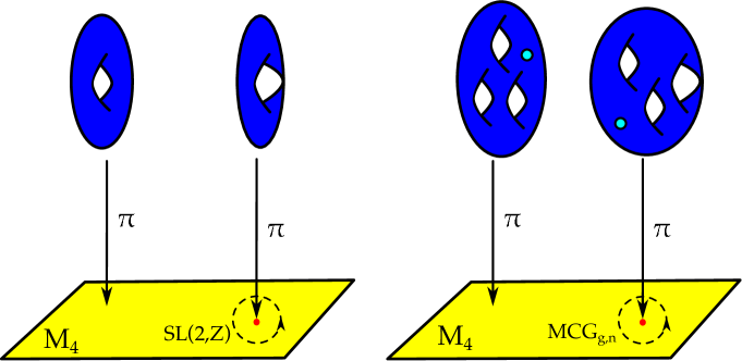
Figure -1379: Theories of Class F: A sketch of the structure of the 6d space-time for the $(2,0)$ theory, which upon reduction along the fibration $\pi$ gives rise to theories of class F, for $T^{2}$ and $C_{3,1}$, respectively, which are 4d theories on $M_{4}$ with varying coupling. Singularities in the fiber result in monodromies of the couplings of the 4d theory, which take values in the mapping class group $\text{MCG}_{g,n}$. On the left hand side this is $SL(2,\mathbb{Z})$. In the class F theories the singular loci correspond to duality defects (shown in red), which are real codimension two in $M_{4}$.

In all the cases a construction of the theories in 4d (unless one considers the abelian theory) will generically result in a non-Lagrangian (or not obviously Lagrangian) theory, which is intrinsically non-perturbative – much like the class S case. A quantity that characterizes the theories, without requiring necessarily a perturbative description is the anomaly polynomial $I_{6}$. We will determine $I_{6}$ for class F theories for both torus and higher genus fibrations by pushforward of the $I_{8}$ anomaly polynomial of the 6d $(2,0)$ theory. In the case of $T^{2}$-fibrations, we can furthermore compare this with a direct anomaly computation for a $U(1)$ symmetry that is related to $SL(2,\mathbb{Z})$ and find agreement. The advantage of the pushforward description is that it captures intrinsically the contributions from the duality defects as well. This will be illustrated for several fibrations.

To substantiate these results we will compare to related configurations, where e.g. D3-branes were studied in the context of F-theory compactifications, either in terms of D3-instantons or wrapped D3-branes, that are strings in the transverse space-time [5, 6, 7, 8, 9, 10, 11, 12]. The 2d SCFTs obtained from wrapped D3-branes have 2d $(0,4)$ or $(0,2)$ supersymmetry and are dimensional reductions of class F where the elliptic fibration $\mathcal{F}$ is non-trivial only over a curve $\Sigma\subset M_{4}$. We determine the dimensional reduction of the class F anomaly polynomial and compare with the known $I_{4}$ anomaly polynomials of these 2d SCFTs.

To provide more depth to this proposal, let us discuss class F in the case of $C=T^{2}$ in some more detail. This theory has an intrinsically 4d description in terms of 4d $\mathcal{N}=4$ SYM, with space-time dependent $\tau$ and with duality defects of complex codimension one, around which $\tau$ undergoes $SL(2,\mathbb{Z})$ monodromies. Alternatively, it is the 6d $(2,0)$ theory on an elliptic fibration with total space $M_{6}$

$$T^{2}\hookrightarrow M_{6}\stackrel{{\scriptstyle\pi}}{{\longrightarrow}}M_{4}\,,$$ (1.2)

where the complex structure of $T^{2}$ is $\tau$ and $M_{4}$ is the 4d space-time (this can be compact or non-compact, Euclidean or Lorentzian). One defining datum of an elliptic fibration [13] is the Weierstrass line bundle $\mathbb{L}$ on $M_{4}$, which is trivial when the fibration is a product, as well as the Weierstrass equation $y^{2}=x^{3}+fx+g$, determined by $f$ and $g$, which are sections of powers of $\mathbb{L}$ and thus position dependent on $M_{4}$. In summary, the data defining this theory of class F is

$$\mathcal{F}=\{\mathbb{L},f,g\}\,.$$ (1.3)

Alternatively we can characterize these class F theories in terms of $\mathcal{N}=4$ SYM, where the complexified gauge coupling $\tau$ varies according to the complex structure of the elliptic curve specified by the Weierstrass model, and has duality defects that are characterized in terms of

$$\boxed{\ T\left[T^{2},\{\mathbb{L},f,g\};G\right]\quad\equiv\quad\hbox{4d $\mathcal{N}=4$ SYM, gauge group $G$, $\tau=\tau(f,g)$, duality defects\ }}$$ (1.4)

The duality defects are located along 2d subspaces of $M_{4}$, above which the $T^{2}$-fiber degenerates. The type of singular $T^{2}$-fiber furthermore encodes (and in fact classifies) the duality defects (see figure -1379).

The local $U(1)$ symmetry associated with the line bundle has a field theoretic interpretation in 4d $\mathcal{N}=4$, where it is a chiral rotation, that the fermions undergo when applying a duality transformation in $SL(2,\mathbb{Z})$ to the theory [14, 15, 5, 7]. The duality acts on the complexified coupling of $\mathcal{N}=4$ SYM by

$$\tau\rightarrow{a\tau+b\over c\tau+d}\,,\qquad\gamma=\begin{pmatrix}a&b\\ c&d\end{pmatrix}\in SL(2,\mathbb{Z})\,,$$ (1.5)

and needs to be accompanied by a $U(1)_{D}$ rotation on the fermions (and supercharges)

$$U(1)_{D}:\qquad e^{i\alpha_{\gamma}(x)}={|c\tau+d|\over c\tau+d}\,.$$ (1.6)

This $U(1)_{D}$ is gauged and defines a line bundle $\mathcal{L}_{D}$, with connection that locally takes the form $Q=-{d\tau_{1}\over 2\tau_{2}}$. Chiral fermions in the vector multiplet are charged under this $U(1)_{D}$ and give rise to a triangle anomaly. We compute the associated $c_{1}(\mathcal{L}_{D})$ dependent terms in the anomaly polynomial $I_{6}$ of 4d $\mathcal{N}=4$ SYM, and show that these include the anomaly

$$\int_{M_{4}}\Sigma(x)\,\text{tr}R\wedge R\,,$$ (1.7)

where $\Sigma(x)$ is the parameter of the $U(1)_{D}$ gauge transformation in (1.6), as was noted in [14]. We show that there are two additional contributions to the anomaly: one is relevant when there is a non-trivial normal bundle, and depends on the R-symmetry bundle, the other is an explicitly $c_{1}(\mathcal{L}_{D})$-dependent term. The conclusion is that the anomaly polynomial of 4d $\mathcal{N}=4$ Super-Yang–Mills on $M_{4}$ with gauge group $G$ has new $c_{1}(\mathcal{L}_{D})$-dependent terms

$$\hbox{{4d $\mathcal{N}=4$ SYM}:}\qquad\quad\begin{aligned} I_{6}=&\ \frac{1}{2}d_{G}c_{3}(\mathcal{S}_{6}^{+})-\frac{1}{2}r_{G}c_{2}(\mathcal{S}_{6}^{+})c_{1}(\mathcal{L}_{D})+\frac{1}{4}r_{G}p_{1}(M_{4})c_{1}(\mathcal{L_{D}})\cr&-\frac{61}{4}r_{G}c_{1}(\mathcal{L}_{D})^{3}\,,\end{aligned}$$ (1.8)

where $\mathcal{S}_{6}^{+}$ is the positive chirality representation of the $SO(6)$ R-symmetry bundle and

$${c_{1}(\mathcal{L}_{D})=\frac{F_{D}}{2\pi}}$$ (1.9)

is the curvature of the connection for the $U(1)_{D}$ bundle. This expression includes the contribution to the anomaly from the duality defects, which are most easily determined by starting in 6d and reducing along the $T^{2}$ fiber. The gauge group data entering the expression are the rank $r_{G}$ and dimension $d_{G}$. These terms become relevant for the class F theories, which have a non-trivial $F_{D}$ background, sourced by a space-time depending $\tau$. The gauge group data entering the anomaly polynomial, the rank and dimension, are invariant under the mapping of $G$ to its Langlands dual group ${}^{L}G$ under an S-duality transformation.

Alternatively, following from the definition of class F starting in 6d, we can compute the anomaly by pushforward of the $I_{8}$ anomaly polynomial of the 6d $(2,0)$ theory along the fiber of the fibration (1.2) and find agreement

$$\pi_{*}I_{8}=I_{6}\,,$$ (1.10)

under the identification of the $U(1)_{D}$ line bundle $\mathcal{L}_{D}$ with the Weierstrass bundle $\mathbb{L}$

$$\mathcal{L}_{D}=\mathbb{L}\,.$$ (1.11)

Once the Weierstrass line $\mathbb{L}$ bundle is fixed, the terms in the first line of (1.8) are independent of the choice of $f$ and $g$ and thus in particular of the specific $\tau$-profile. We shall refer to such terms, that are independent of $f$ and $g$ as $\mathbb{L}$-universal – though often we will abbreviate this to simply universal.

The $c_{1}(\mathcal{L}_{D})^{3}$ term, as we will discuss later on, depends on the number of sections that the elliptic fibration has. Furthermore there can be terms arising from defects that carry non-abelian flavor symmetries, which are again dependent on the specific fibration. The reader is referred to section 5.3 for the precise form of these additional terms. We derive these contributions from duality defects by a careful analysis of the pushforward of $I_{8}$ for singular elliptic fibrations: the Kodaira singularity type determines the flavor symmetries $G_{F}$ of the duality defects [7], and the corresponding terms to $I_{6}$ in the presence of duality defects that are localized along a surface $S_{G_{F}}$ are

$$I_{6}^{\text{duality defects}}={\mathfrak{a}_{2}\over 4}\,c_{1}(\mathbb{L})^{2}S_{G_{F}}-{\mathfrak{a}_{1}\over 8}c_{1}(\mathbb{L})\,S_{G_{F}}^{2}+{\mathfrak{a}_{0}\over 4}\,S_{G_{F}}^{3}\,,$$ (1.12)

where $\mathfrak{a}_{i}$ depend on the singularity type/flavor symmetry and are determined in section 5.3. Here we think of the 6d space-time as a complex three-fold and $S_{G_{F}}$ is a divisor (dual to a 2-form). In fact this implies that duality defects for class F with $T^{2}$ fibers are classified in terms of the Kodaira classification of singular elliptic fibers [16].

Class F with higher genus curves can be discussed in a similar way starting in 6d. We explore in this paper the case of no punctures and fibrations that are realized in terms of projective bundles as plane-curve fibrations. We find a similar generalization of the anomaly polynomial of class S [17, 18] to include correction terms, see (5.25). In this case the only way we can so far analyze this is starting in 6d, and it would indeed be interesting to complement this with an intrinsically 4d analysis, much like in the $\mathcal{N}=4$ SYM case. We should remark that these corrections to the anomaly polynomial are complementary to the ones discussed recently, with terms depending on forms on the moduli space of the couplings of the theory [19, 20]. The terms we obtain become relevant when the coupling becomes dependent on physical space-time. As mentioned earlier, punctures will correspond to sections of the fibrations, which carry additional representation theoretic data. For elliptic fibrations, models with small number of sections are well-understood and can be studied systematically. For higher genus, already models with one section will correspond to extra data. Generalizing the derivation of the anomaly polynomials will be possible by combining the methods of the present paper with those developed for class S with punctures in [21], which will be discussed elsewhere. We will in the following abbreviate $C_{g}\equiv C_{g,0}$.

The plan of the paper is as follows: we begin by defining theories of class F in section 2. In section 3 we discuss the origin of the $U(1)_{D}$ symmetry from 6d as well as in 4d $\mathcal{N}=4$ SYM, and its generalization to higher genus. We then derive the anomaly terms for 4d $\mathcal{N}=4$ SYM that are $U(1)_{D}$ dependent from a field theory point of view in section 4. This is complemented in section 5 by a pushforward of the 6d anomaly polynomial along the fiber, which we discuss for both $g=1$ and $g>1$, as well as the contributions from duality defects. We check our results against known expressions for anomaly polynomials of 2d theories arising from D3-branes wrapped on curves in F-theory compactifications in section 6. Finally, some extensions beyond class F are discussed in section 7, in particular to the non-supersymmetric case of 6d self-dual tensor and 4d Maxwell theory, class S and $\mathcal{N}=1$ theories in 4d with space-time-dependent coupling. We conclude in section 8 and provide several appendices with details of conventions and computations.

2 Theories of Class F

2.1 F is for Fiber

Theories of class S are 4d $\mathcal{N}=2$ theories defined as dimensional reductions with a topological twist of the 6d $(2,0)$ SCFTs with gauge group $G$ on a Riemann surface $C_{g,n}$, of genus $g$ with $n$ punctures [1]. The different pair of pants decompositions of the curve correspond to different duality frames of the 4d theories. The simplest precursor of this is the 4d $\mathcal{N}=4$ theory, which is the 6d $(2,0)$ theory on a $T^{2}=\mathbb{E}_{\tau}$, an elliptic curve, whose complex structure is identified as

$$\tau={\theta\over 2\pi}+i{4\pi\over g^{2}}\,.$$ (2.1)

The duality group is $SL(2,\mathbb{Z})$, which acts by modular transformations

$$\tau\rightarrow{a\tau+b\over c\tau+d}\,,\qquad ad-bc=1\,,\quad a,b,c,d\in\mathbb{Z}\,.$$ (2.2)

The type of theories we would like to consider generalize this setup to allow for the curve $C$ to vary over space-time – consistently with the duality symmetries of the theories in 4d. When $C=T^{2}$ is an elliptic curve, some aspects of these theories have been studied in [5, 7], where the 4d space-time was specialized to a compact complex surface, and [6, 8], where the 4d space-time was specialized to $\mathbb{R}^{1,1}\times\Sigma$, with $\Sigma$ a complex curve. For higher genus fibrations a brief discussion has appeared in [22].

Our main focus here will be on the 4d theories on $M_{4}$ and their anomaly polynomials. The data that we will use to define the theories are genus-$g$ fibrations over $M_{4}$

$$\mathcal{F}:\qquad C_{g}\ \hookrightarrow\ M_{6}\ \rightarrow\ M_{4}\,,$$ (2.3)

which geometrically model the profile of the complex couplings of the theory of class S on $M_{4}$. For $g>1$ the theory is defined with a topological twist along the fiber. Subspaces $\Delta\subset M_{4}$, of real codimension two, above which the fibers develop singularities correspond to duality defects, around which the couplings undergo a duality transformation in the mapping class group $\text{MCG}_{g}$ of $C_{g}$.

For $C=T^{2}$, the theory in 4d is $\mathcal{N}=4$ SYM with space-time varying complex coupling $\tau$. The situation in this case is thus very similar to IIB with varying axio-dilaton, i.e. F-theory [2], and indeed the theories obtained in this way can be thought of as the world-volume theories of D3-branes in F-theory, where the axio-dilaton variation descends to the variation of $\tau$. The theory can either be studied via M/F-type duality, where the 6d theory is realized in terms of M5-branes, or directly in terms of a 4d theory with varying coupling $\tau$. The latter point of view is advocated in F-theory in [23], which defines this theory as Type IIB with a fibration, that is specified by a bundle and sections $f$ and $g$ that specify a Weierstrass model.

The theories we will study are a generalization of class S to fibrations and will be referred to as theories of class F: they are obtained by reducing the M5-brane theory on a curve $C$, which however varies over the 4d space-time, allowing for monodromies in duality symmetries of the 4d theory, which are elements of the mapping class group $\text{MCG}_{g}$. The reduction from 6d to 4d is along the fiber of a fibration $C\hookrightarrow M_{6}\rightarrow M_{4}$. The data that defines these theories is the gauge group $G$ of the 6d theory, together with the fibration. Alternatively, in the nomenclature where class S theories are denoted by $T[C_{g};G]$, class F theories are determined by the data

$$T\left[C_{g},\mathcal{F};G\right]\,:\qquad\left\{\begin{aligned} C_{g}\qquad&\text{genus $g$ curve}\cr G\qquad&\text{gauge group of ADE type}\cr\mathcal{F}\qquad&\text{data specifying a genus $g$-fibration over 4d space-time $M_{4}$}\end{aligned}\right.\,.$$ (2.4)

As noted earlier, these are generically not Lagrangian theories. Nevertheless we will be able to compute the anomaly polynomials of the class F theories for $g=1$ and an infinite subclass of higher genus theories. One key ingredient that we will leave for the future are punctures, which will be studied elsewhere.

To fill the description of class F theories with life we will now specify the data required for the fibrations $\mathcal{F}$, and give concrete descriptions of the fibrations in the case $g=1$ and $g>1$, respectively.

2.2 Elliptic Fibrations

We start by exploring $C=T^{2}$ and to emphasize the complex nature will often specify this as an elliptic curve $\mathbb{E}_{\tau}=\mathbb{C}/\mathbb{Z}\oplus\tau\mathbb{Z}$. The class F theories of this type are characterized by the data

$$T\left[\mathbb{E}_{\tau},\mathcal{F};G\right]\,,\qquad\mathcal{F}=\{\mathbb{L},f,g\}\,,$$ (2.5)

where $\mathbb{L}$ is a line bundle

$$\mathbb{L}\rightarrow M_{4}\,,$$ (2.6)

such that there are sections

$$f\in H^{0}\left(\mathbb{L}^{4}\right)\,,\qquad g\in H^{0}\left(\mathbb{L}^{6}\right)\,,$$ (2.7)

and $G$ is the gauge group in 6d. In this description we assume the fibration to have a section (a map from $M_{4}$ to the fiber), and thus a description in terms of a Weierstrass equation

$$y^{2}=x^{3}+fx+g\,.$$ (2.8)

This provides the total space of the fibration $M_{6}$ with a description in terms of an elliptic fibration over $M_{4}$. For trivial fibrations (i.e. $\mathbb{L}=\mathcal{O}$), the theory reduces to the standard 4d $\mathcal{N}=4$ SYM theory with gauge group $G$ on $M_{4}$ with coupling $\tau$ given by the complex structure of the fixed elliptic curve.

We will begin with $G=U(1)$ where the theory can be understood completely explicitly [7] as a dimensional reduction of the tensor multiplet. Starting with the 6d $(2,0)$ theory we see that there are two aspects to these 4d theories – already noted in [7]: the “bulk” part of the spectrum, obtained from the reduction of the tensor multiplet, which results in a 4d $\mathcal{N}=4$ theory with varying coupling. The second contribution arises from singular fibers – i.e. they are localized defect modes above which the elliptic fiber becomes singular. In terms of the data in (2.5) this locus is given by the subspaces in $M_{4}$ that satisfy

$$\Delta=4f^{3}+27g^{2}=0\,.$$ (2.9)

It is important to note that the 4d space-time $M_{4}$ can be compact or non-compact.

Alternatively we define class F theories with $C=T^{2}$ directly in 4d, as 4d $\mathcal{N}=4$ SYM with varying coupling, which is consistent with the $SL(2,\mathbb{Z})$ duality group. Again this requires specifying a line bundle $\mathcal{L}_{D}$ and sections $f$ and $g$, which determine the $\tau$-profile along $M_{4}$. In some cases the coupling will only vary over part of the 4d space-time $M_{4}$. We will at times indicate the subspace where the coupling varies by superscribing it with $\tau$

$$M_{4}=S^{\tau}\quad\hbox{or}\quad S^{\tau}\times\mathbb{R}^{1,1}\,,$$ (2.10)

where $S^{\tau}$ is embedded into the base of an elliptic fibration. Concretely, either $S^{\tau}=\Sigma$, a complex curve, which will be studied in section 6, or $S^{\tau}=D$, a complex surface.

2.3 Fibrations by Genus $g>1$ Curves

Class F which generalizes class S theories, are constructed from fibrations by genus $g$ curves $C_{g}$. There is no canonical realization as in the elliptic case, however we will consider for simplicity here the case of plane curve fibrations. For genus $g$ fibrations, the monodromies around singular fibers are in the mapping class group $\text{MCG}_{g}$. We can in principle include punctures, as additional data on the curve, but in this paper we will refrain from doing so. To be able to define the fibration, $M_{4}$ will have a complex structure, at least on the subspace of $M_{4}$ over which the fibration is non-trivial. The total space can be realized as a hypersurface in a projective bundle, for which the following data is required:

$$\mathcal{F}=\left\{\begin{aligned} \mathcal{J}\rightarrow M_{4}:&\qquad\text{line bundle over $M_{4}$}\cr\varpi=(a,b,d,e)\in\mathbb{Z}^{4}\cr\mathbb{P}\mathcal{E}=\mathbb{P}(\mathcal{O}\oplus\mathcal{J}^{a}\oplus\mathcal{J}^{b}):&\qquad\text{projective bundle over $M_{4}$}\cr Y_{\varpi}=0:&\qquad\text{hypersurface equation in $\mathbb{P}\mathcal{E}$ with}\ [Y_{\varpi}]=d\,H+e\,c_{1}(\mathcal{J})\,.\end{aligned}\right.$$ (2.11)

Here $H$ is the hyperplane class of $\mathbb{P}\mathcal{E}$. This gives a plane-curve fibration where the genus is related to the degree $d$ by

$$g={(d-1)(d-2)\over 2}\,.$$ (2.12)

This does not realize all genera, in particular this does not include the case $g=2$. Genus 2 curves are hyperelliptic and can be realized in terms of a similar construction to the above, and a partial list of singular fibers was determined by Ogg and Namikawa–Ueno [24, 25]. More generally, genus $g$ fibrations have a description as Lefschetz fibrations (over 4d base spaces). This description will be useful in particular for studying the duality symmetries, however in this paper our focus is to determine the anomaly polyomials for such theories, which require us to be able to pushforward forms along the fiber. Such a description is known to us explicitly only for hypersurfaces in projective bundles, as given above.

Obviously, plane curve fibrations specialize to the elliptic case. Indeed from (2.12) for $g=1$ and $\varpi=(2,3,3,6)$ this corresponds precisely to the smooth Weierstrass model for an elliptic Calabi-Yau, with $\mathcal{J}=\mathbb{L}$. Fibrations with multiple sections can also be realized, e.g. $\varpi=(1,1,3,3)$ corresponds to the two-section model.

3 $U(1)_{D}$ Symmetry of Class F Theories

The class F constructions introduced in the last section by elliptic or plane-curve fibrations are each based on a line bundle. We will now see that the connection on this line bundle corresponds to a $U(1)_{D}$ connection in the 4d theory, which is sourced by the space-time dependent coupling. In the simplest case of $C=T^{2}$, writing $\tau=\tau_{1}+i\tau_{2}$, this connection is

$$Q=-\frac{1}{2\tau_{2}}d\tau_{1}\,.$$ (3.1)

In this section we will explain the origin of this $U(1)_{D}$, from 6d, where it is related to the local Lorentz symmetry of the fibral curve, or directly in 4d. This $U(1)_{D}$ will play a key role in that it is anomalous and we will show that the anomaly polynomials for 4d $\mathcal{N}=4$ and class S, have corrections depending on the non-trivial curvature of a $U(1)_{D}$ line bundle. These terms are non-zero whenever we extend these theories to varying coupling, i.e. to class F.

3.1 $U(1)_{D}$ from 6d $(2,0)$

We are considering the 6d $(2,0)$ theory on a complex threefold with a fibration structure, $\pi:M_{6}\rightarrow M_{4}$, where $M_{4}$ is a (not necessarily compact) complex surface. We will assume furthermore, that the threefold is Kähler. The tangent bundle $TM_{6}$ to $M_{6}$ has reduced holonomy $SU(3)_{L}\times U(1)_{L}$, likewise the holonomy of $TM_{4}$ is $SU(2)_{l}\times U(1)_{l}$.

Each of these tangent bundles admits a spin connection, $\Omega$ and $\omega$ respectively, and the curvature associated to the $U(1)$ parts of these connections are, respectively, $\mathcal{R}_{M_{6}}$ and $\mathcal{R}_{M_{4}}$, such that (see appendix A for our conventions)

$$c_{1}(M_{n})=\frac{1}{2\pi}\mathcal{R}_{M_{n}}\,.$$ (3.2)

When considering a fibration by genus $g$ curves $\pi:M_{6}\rightarrow M_{4}$ there exists a short exact sequence defining the (rank one) relative tangent bundle

$$0\rightarrow T_{M_{6}/M_{4}}\rightarrow TM_{6}\rightarrow\pi^{*}TM_{4}\otimes I_{X}\rightarrow 0\,,$$ (3.3)

where $I_{X}$ is a sheaf supported on the singular fibers of the fibration, and which we shall suppress the details of in the following. As such we can see that the above curvatures on the two tangent bundles, $TM_{6}$ and $TM_{4}$ are related through

$$c_{1}(M_{6})=c_{1}(M_{4})+c_{1}(T_{M_{6}/M_{4}})+\cdots\,,$$ (3.4)

where from now on we will suppress the pullback on the $c_{1}(M_{4})$. In this way we can see that the $U(1)$ part of the spin connection on $M_{6}$ decomposes as

$$\Omega=\omega+\mathcal{A}+\cdots\,,$$ (3.5)

where $\mathcal{A}$ is a connection one-form on $T_{M_{6}/M_{4}}$. For genus one fibrations, we have

$$T_{M_{6}/M_{4}}=\pi^{*}\mathbb{L}^{\vee}\,,$$ (3.6)

and thus we identify the connection $\mathcal{A}$ with $(-Q)$, the connection on the dual of the Weierstrass line bundle $\mathbb{L}$. This is the vector potential for the local $U(1)_{D}$ abelian symmetry, as was determined explicitly in [7]. It was furthermore shown there that the connection is precisely the one in (3.1).

For $g>1$, $T_{M_{6}/M_{4}}$ has a more complicated structure, as $TC_{g}$ is a non-trivial bundle, and the gauge connection for the $U(1)_{D}$ bundle will be mixed, in $\mathcal{A}$, with the potential $\mathcal{A}_{g}$ for the $SO(2)$ holonomy of $C_{g}$. To see this, consider the case of a product space $M_{4}\times C_{g}$, then $T_{M_{6}/M_{4}}$ is just $TC_{g}$, namely $\mathcal{A}=\mathcal{A}_{g}$. We do not have a universal formulation for genus $g$ fibrations, however for the plane curve fibration introduced in section 2.3 the canonical class of the hypersurface fibration is

$$K_{Y_{\bar{w}}}=\pi^{*}\left((e-a-b)c_{1}(\mathcal{J})-c_{1}(M_{4})\right)+(3-d)c_{1}(\mathcal{O}_{\mathbb{P}(\mathcal{E})}(1))\,,$$ (3.7)

and the relative tangent bundle of such fibrations can be seen to contain a factor of $\mathcal{J}$,

$$T_{M_{6}/M_{4}}=\left(\pi^{*}\mathcal{J}^{-(e-a-b)}\right)\otimes{\mathcal{R}}\,,$$ (3.8)

the connection of which is expected to be the $U(1)_{D}$ connection, and where this equation defines $\mathcal{R}$. The pushforward of the relative tangent bundle is rank $g$, which follows since rank$(T_{M_{6}/M_{4}})=1$, as the fiber is a complex curve, and the pushforward of the vector bundle is the rank of the original bundle with multiplicity given by the degree of the morphism, which is $g$. From (3.8) and the projection formula it follows that $\pi_{*}T_{M_{6}/M_{4}}=\mathcal{J}^{-(e-a-b)}\otimes\pi_{*}(\mathcal{R})$, where the pushforward $\pi_{*}(\mathcal{R})$ is a rank $g$ bundle. Notice that for $\varpi=(2,3,3,6)$ the relation (3.8) reduces precisely to (3.6), where the bundle $\mathcal{R}$ is trivial.

3.2 $U(1)_{D}$ in 4d

In the case of class F theories of type $T[T^{2},\mathcal{F}]$ the discussion of the $U(1)_{D}$ from 6d can be complemented with a direct analysis in 4d. The situation is reminiscent to Type IIB with a non-trivial axio-dilaton background, where the supergravity background scalars parametrize the coset $SL(2,\mathbb{R})/U(1)$ [26, 27]. In this case the ungauge-fixed version of the Type IIB theory has three scalars parametrizing $SL(2,\mathbb{R})$ and the chiral fermions transform under a local $U(1)$ symmetry, which upon gauge fixing is identified with $U(1)\subset SL(2,\mathbb{R})$. This gauge fixing removes one of the three scalars, but for this gauge condition to be preserved under a general $SL(2,\mathbb{R})$ transformation, these have to be accompanied with a compensating $U(1)$-transformation, which acts non-trivially on the fermions – in this way an $SL(2,\mathbb{R})$ transformation induces a $U(1)$ action on the fermions. This $U(1)_{D}$ plays a fundamental role in formulating F-theory, i.e. Type IIB with varying axio-dilaton.

A very similar situation arises in 4d $\mathcal{N}=4$ SYM, where again there are background fields that parametrize $SL(2,\mathbb{R})/U(1)$, and it is the anomaly of this $U(1)$ symmetry that we will discuss in the following. From a 4d point of view the varying $\tau$ background is realized by coupling the theory to a non-dynamical off-shell supergravity multiplet [28], in this case we couple to $\mathcal{N}=4$ conformal supergravity [29]. This supergravity has an $SL(2,\mathbb{R})$ global and $U(1)$ local symmetry: the scalar manifold has three scalars $\tau_{1},\tau_{2},\phi$, which parametrize an element of $SL(2,\mathbb{R})$ by

$$\Phi={1\over\sqrt{\tau_{2}}}\begin{pmatrix}\tau_{2}\cos\phi+\tau_{2}\sin\phi&-\tau_{2}\sin\phi+\tau_{1}\cos\phi\\ \sin\phi&\cos\phi\end{pmatrix}\in SL(2,\mathbb{R})\,.$$ (3.9)

The symmetries $h\in SL(2,\mathbb{R})$ and $R(\alpha_{\gamma}(x))\in U(1)$ act by

$$\Phi\rightarrow h\Phi\begin{pmatrix}\cos\alpha_{\gamma}&\sin\alpha_{\gamma}\\ -\sin\alpha_{\gamma}&\cos\alpha_{\gamma}\end{pmatrix}\,.$$ (3.10)

A useful gauge fixing of the $U(1)$ was described in [14] in analogy to the one in IIB [26], by fixing $\phi=0$ (under the local $U(1)$ this shifts by $\phi\rightarrow\phi+\Sigma$), and identifies $\Phi$ with the complexified coupling $\tau$, which takes values in the coset $SL(2,\mathbb{R})/U(1)$. This gauge choice is invariant under $SL(2,\mathbb{R})\times U(1)$ only with the additional compensating (local) $U(1)$ transformation

$$U(1)_{D}:\qquad e^{i\alpha_{\gamma}(x)}={|c\tau+d|\over c\tau+d}\,,$$ (3.11)

where $h\tau={a\tau+b\over c\tau+d}$, and this acts by shift on $\phi$, and a phase rotation on the fermions. This is precisely the $U(1)_{D}$ symmetry that also descends from 6d [7], and was observed to be relevant for S-duality transformations of 4d $\mathcal{N}=4$ SYM in [15]. The gauge potential for the local $U(1)_{D}$ symmetry is

$$\partial_{\mu}\phi+Q_{\mu}=\partial_{\mu}\phi-{\partial_{\mu}\tau_{1}\over 2\tau_{2}}\,,$$ (3.12)

which is precisely the one obtained earlier from 6d in (3.1). There is triangle anomaly for the $U(1)_{D}$ current, involving the gauginos in the loop which transform under the $U(1)$ symmetry. One such contribution was computed in [14], in the case of trivial normal bundle, where it was shown that the D3-brane on $M_{4}$ has an anomaly under the $U(1)$ symmetry, arising from the coupling to gravitons, of the form

$$\delta S_{\text{gauginos}}\propto\int_{M_{4}}\Sigma(x)\,p_{1}(M_{4})\,,$$ (3.13)

where as before $\Sigma$ is the gauge variation of $\phi$ under the local $U(1)$ transformation. Such an anomalous variation is cancelled by the addition of a counterterm to the 4d action

$$S_{ct}=\int_{M_{4}}\phi\,p_{1}(M_{4})\,.$$ (3.14)

In this paper we extend this result to include a non-trivial R-symmetry bundle, and to include $U(1)^{3}$ anomalies, and in addition we study the contribution to the $U(1)$ anomalies, not just of the bulk $\mathcal{N}=4$ gauginos, but also those from the degrees of freedom living on the duality defects when $\tau$ varies holomorphically along $M_{4}$.

The classical $SL(2,\mathbb{R})$ is broken to $SL(2,\mathbb{Z})$ quantum mechanically, and in fact the full duality group has recently been discussed to be the $\mathbb{Z}_{2}$ central extension of $SL(2,\mathbb{Z})$, the metaplectic group [30], see also [23], which includes precisely also the action on the fermions with the phase rotation with half-integral charge.

4 4d $\mathcal{N}=4$ and the $U(1)_{D}$ Anomaly

This section will be entirely about class F theories with $C=T^{2}$. We begin by discussing the anomaly in $\mathcal{N}=4$ SYM in 4d associated to the $U(1)_{D}$ symmetry. This is a priori independent of the class F construction from 6d, but what we will see is that there are additional terms in the anomaly polynomial for $\mathcal{N}=4$ SYM that become relevant whenever there is a non-trivial $U(1)_{D}$ connection, as in the case of class F.

We first review the action of the $U(1)_{D}$ introduced in section 3 on the chiral fermions in the $\mathcal{N}=4$ vector multiplet, and then compute the one-loop anomaly arising from the chiral fermions on the generic point of the Coulomb branch of any $\mathcal{N}=4$ SYM theory, and use ’t Hooft anomaly matching to relate to the anomaly at the origin of the Coulomb branch. This involves a conjecture that any interaction terms in the effective theory when integrating out the massive fermions and moving onto the Coulomb branch are irrelevant for any $U(1)_{D}$-related anomaly. This is because we expect that the interaction terms will provide a contribution to the anomaly polynomial proportional to the number of massive W-bosons on the Coulomb branch; in section 5 we will see that any contributions to the $U(1)_{D}$ anomalies that scale in such a way will be at odds with the point of view from the 6d $(2,0)$ superconformal field theory.

4.1 Anomaly Polynomial for 4d $\mathcal{N}=4$ SYM with Gauged $U(1)_{D}$

The $U(1)_{D}$ symmetry of $\mathcal{N}=4$ SYM discussed in section 3, arising from the $SL(2,\mathbb{R})\times U(1)$ enhanced symmetry when coupling the 4d theory to an arbitrary supergravity background, can be seen to act as an R-symmetry of the superconformal group $PSU(2,2|4)$. In [31, 32] it was shown that $PSU(2,2|4)$ admits such an outer automorphism. For the abelian 4d $\mathcal{N}=4$ SYM theory, this gives rise to a symmetry of the spectrum of some observables, though not of the Lagrangian [31]. The gauginos transform under the bosonic subgroup $Spin(1,3)\times SU(4)_{R}$ of $PSU(2,2|4)$ and the duality $U(1)_{D}$ as follows

$$({\bf 2,1,4})_{1/2}\oplus({\bf 1,2,\overline{4}})_{-1/2}\,.$$ (4.1)

As such, we can compute the anomalies of the $U(1)_{D}$ symmetry in the usual way, specifically we use the Wess–Zumino descent procedure (for reviews on this topic see e.g. [33]), where the anomaly due to a chiral fermion transforming in a representation ${\bf R}$ of a group $G$ is determined via the anomaly (4+2)-form

$$\left.\hbox{ch}(F_{\bf R})\widehat{A}(TM_{4})\right|_{6\text{-form}}\,,$$ (4.2)

where $TM_{4}$ is the tangent bundle to the 4d space-time, $M_{4}$. Applied to 4d $\mathcal{N}=4$ SYM via the fermions in (4.1) this results in

$$\frac{1}{2}\left(\hbox{ch}(\mathcal{S}_{6}^{+}\otimes\mathcal{L}_{D}^{1/2})-\hbox{ch}(\mathcal{S}_{6}^{-}\otimes\mathcal{L}_{D}^{-1/2})\right)\widehat{A}(TM_{4})=\hbox{ch}(\mathcal{S}_{6}^{+}\otimes\mathcal{L}_{D}^{1/2})\widehat{A}(TM_{4})\,,$$ (4.3)

where $\mathcal{S}_{6}^{\pm}$ are the complex conjugate vector bundles associated to the ${\bf 4}$, ${\bf\overline{4}}$ of $SU(4)_{R}$, and $\mathcal{L}_{D}$ is the bundle associated to the charge $+1$ representation of $U(1)_{D}$. $\mathcal{L}_{D}$ is the bundle with connection (3.1). This connection e.g. can be derived by considering a supergravity background for the 4d $\mathcal{N}=4$ theory with a non-trivial $\tau$ profile [5, 34, 9]. If the coupling does not vary over space-time, the bundle $\mathcal{L}_{D}$ is trivial and we recover the expected result for the anomaly polynomial for constant coupling $\mathcal{N}=4$ SYM.

We can now compute the anomaly polynomials, starting with the abelian theory $G=U(1)$. Expanding out the characteristic classes in (4.3), for a summary of our conventions see appendix A, one finds that the contribution to the anomaly from the gauginos in the $U(1)$ $\mathcal{N}=4$ vector multiplet is

$$I_{6}^{F}=\frac{1}{2}c_{3}(\mathcal{S}_{6}^{+})-\frac{1}{2}c_{2}(\mathcal{S}_{6}^{+})c_{1}(\mathcal{L}_{D})+\frac{1}{12}c_{1}(\mathcal{L}_{D})^{3}-\frac{1}{12}p_{1}(TM_{4})c_{1}(\mathcal{L}_{D})\,.$$ (4.4)

The first term is the standard contribution due to the R-symmetry $SU(4)_{R}$ anomaly. The remaining terms are explicitly $\mathcal{L}_{D}$ dependent and signal anomalies due to gauging $U(1)_{D}$.

To generalize this to a $U(N)$ gauge group we first consider the theory in a Higgsed phase. On the Coulomb branch of the $U(N)$ theory the gauge group is $U(1)^{N}$ and the total number of massless Weyl fermions is $4N$, where $N$ is the rank of the Cartan subalgebra. As such the anomaly contribution is simply $N\times I_{6}^{F}$. However, this is not the whole story, as described in [35], there are Wess–Zumino interaction terms that are induced in integrating out the massive states when moving onto the Coulomb branch, and these will modify the anomaly polynomial even deep on the Coulomb branch. We shall assume that, also in the case of a space-time dependent $\tau$, these Wess–Zumino terms introduce the same contribution to the anomaly polynomial as in the constant $\tau$ case, to wit,

$$I_{6}^{WZ}=\frac{1}{2}(N^{2}-N)c_{3}(\mathcal{S}_{6}^{+})\,.$$ (4.5)

As such, the anomaly polynomial of $U(N)$ $\mathcal{N}=4$ SYM arising from the bulk degrees of freedom is conjectured to be

$$I_{6} =NI_{6}^{F}+I_{6}^{WZ}$$ (4.6)

$$=\frac{1}{2}N^{2}c_{3}(\mathcal{S}_{6}^{+})-\frac{1}{2}Nc_{2}(\mathcal{S}_{6}^{+})c_{1}(\mathcal{L}_{D})+\frac{1}{12}Nc_{1}(\mathcal{L}_{D})^{3}-\frac{1}{12}Np_{1}({TM_{4}})c_{1}(\mathcal{L}_{D})\,.$$

As described in section 2, there are in addition to the bulk modes, localised defect degrees of freedom in the theory with non-trivial $\mathcal{L}_{D}$, and these will further contribute to the anomaly polynomial. We will compare (4.6) in the next section to the ’t Hooft anomaly coefficients.

4.2 ’t Hooft Anomaly Coefficients

Alternatively we can compute the ’t Hooft anomaly coefficients directly on the Coulomb branch of the $G=U(N)$ $\mathcal{N}=4$ SYM [35], which consists of $N$ massless $\mathcal{N}=4$ $U(1)$ vector multiplets, each of which can be written in $\mathcal{N}=1$ language as a vector multiplet, $V$, and three chiral multiplets, $\Phi_{i}$. The R-charges of these multiplets are

$$R[V]=1\,,\quad R[\Phi_{i}]=\frac{2}{3}\,.$$ (4.7)

The R-charge of three adjoint scalars $\Phi_{i}$ is fixed by requiring the cubic superpotential to have R-charge 2, while the R-charge of the vector multiplet is such that the gauge field is uncharged. Equivalently, these charges can be derived by decomposing the $SU(4)$ R-symmetry as follows. Let us consider the fermions in the representation $({\bf 2,1,4})$ under $SO(1,3)\times SU(4)_{R}$. First we consider the decomposition to the R-symmetry of an $\mathcal{N}=2$ subalgebra

$$SU(4) \rightarrow SU(2)_{R}\times SU(2)_{L}\times U(1)_{R}$$ (4.8)

$${\bf 4} \rightarrow({\bf 2,1})_{1}\oplus({\bf 1,2})_{-1}\,,$$

where $SU(2)_{R}\times U(1)_{R}$ now forms the R-symmetry of the $\mathcal{N}=2$ SCFT. We can now apply the relation between the $\mathcal{N}=2$ R-symmetry and the $\mathcal{N}=1$ R-charge,

$$R_{\mathcal{N}=1}=\frac{1}{3}R_{\mathcal{N}=2}+\frac{4}{3}L_{3}\,,$$ (4.9)

where $L_{a}$ are the generators of the $SU(2)_{R}$ and $L_{3}$ is such that the ${\bf 2}$ has charges $\pm\frac{1}{2}$, to find

$$({\bf 2,1,4})\rightarrow({\bf 2,1})_{1}\oplus({\bf 2,1})_{-1/3}\oplus({\bf 1,2})_{-1/3}\oplus({\bf 1,2})_{-1/3}\,,$$ (4.10)

where the final subscript is the $U(1)_{R}^{\mathcal{N}=1}$ charge. Since the R-charge of the fermions in the chiral multiplets is one less than the charge of the scalar we can see that it follows that (4.7) are the R-charges. Further, since we are considering the fermions in the positive chirality $({\bf 2,1,4})$ representation we must take the $U(1)_{D}$ charge of all the fermions to be

$$q_{D}=\frac{1}{2}\,.$$ (4.11)

The anomaly polynomial of the ${\cal N}=4$ theory takes the form

$$I_{6}= \frac{1}{6}k_{RRR}c_{1}(R)^{3}+\frac{1}{2}k_{RRD}c_{1}(R)^{2}c_{1}({\cal L}_{D})+{\frac{1}{6}}k_{DDD}c_{1}({\cal L}_{D})^{3}-\frac{1}{24}k_{D}c_{1}({\cal L}_{D})p_{1}({TM_{4}})\,,$$ (4.12)

where recall that the ’t Hooft anomaly coefficients are defined as

$$k_{IJK}=\mathop{\mathrm{Tr}}\nolimits_{f_{+}}q_{I}q_{J}q_{K}\,,\qquad k_{I}=\mathop{\mathrm{Tr}}\nolimits_{f_{+}}q_{I}\,,$$ (4.13)

where the trace is taken over all positive chirality Weyl fermions, and we have written only the non-zero terms. In particular, the following quantities may be computed directly from the field content

$$k_{R} =N\left(3\times\left(-\frac{1}{3}\right)+1\times 1\right)=0$$ (4.14)

$$k_{RRR} =N\left(3\times\left(-\frac{1}{3}\right)^{3}+1\times 1^{3}\right)=\frac{8}{9}N$$

$$k_{D} =N\left(4\times\left(\frac{1}{2}\right)\right)=2N$$

$$k_{RRD} =N\left(3\times\left(-\frac{1}{3}\right)^{2}\left(\frac{1}{2}\right)+1\times 1^{2}\left(\frac{1}{2}\right)\right)=\frac{2}{3}N$$

$$k_{RDD} =N\left(3\times\left(-\frac{1}{3}\right)\left(\frac{1}{2}\right)^{2}+1\times 1\left(\frac{1}{2}\right)^{2}\right)=0$$

$$k_{DDD} =N\left(4\times\left(\frac{1}{2}\right)^{3}\right)=\frac{1}{2}N\,.$$

As explained previously, Wess–Zumino terms are introduced via the integrating out of the massive modes as one moves onto the Coulomb branch, these couplings contribute to the $k_{RRR}$ ’t Hooft anomaly coefficient like

$$n_{V}\times(\text{contribution from single fermion in ${\bf 4}$})=\frac{8}{9}(N^{2}-N)\,,$$ (4.15)

where $n_{V}$ is the number of massive fermions. Thus the total $k_{RRR}$ anomaly coefficient can be calculated on the Coulomb branch to be

$$k_{RRR}=\frac{8}{9}N+\frac{8}{9}(N^{2}-N)=\frac{8}{9}N^{2}\,.$$ (4.16)

For $\mathcal{N}=4$ super-Yang–Mills we can use the relationship between the central charges and the ’t Hooft anomaly coefficients

$$a=\frac{9}{32}k_{RRR}-\frac{3}{32}k_{R}\,,\quad c=\frac{9}{32}k_{RRR}-\frac{5}{32}k_{R}\,,$$ (4.17)

to determine the central charges for $G=U(N)$ to be

$$a=c=\frac{1}{4}N^{2}\,.$$ (4.18)

It can be verified that, upon rewriting the $SU(4)_{R}$ in term of the $U(1)_{R}^{\mathcal{N}=1}$, the ’t Hooft anomalies computed from the field content in (4.14) match exactly with those in (4.6).

4.3 Modular Anomaly Revisited

The Montonen–Olive duality group of 4d $\mathcal{N}=4$ SYM is $SL(2,\mathbb{Z})$ [38, 39, 40], and under the S-duality transformations of this group the partition function, $Z(\tau)$, is known to transform as a modular form [41, 42]. This failure of invariance of the partition function under the action of the duality group is known as the modular anomaly.

When the $\mathcal{N}=4$ SYM is embedded into string theory, as the worldvolume theory on a stack of D3 branes, it is expected that the modular anomaly, which is then the anomaly of a local $SL(2,\mathbb{Z})$, is cancelled. The putative $SL(2,\mathbb{Z})$ duality group . This subtletly will not concern us in this discussion. of Type IIB string theory, from which descends the $SL(2,\mathbb{Z})$ on the D3-brane, arises as the remnant, after quantisation, of the $SL(2,\mathbb{R})$ global symmetry of Type IIB supergravity. In [14] it was shown, in a particular simple background, that part of the modular anomaly is cancelled by considering the D-instanton corrections to the D3-brane action, together with the counterterm cancelling the local $U(1)$ anomaly discussed in section 3.2. In this case the remaining part of the modular anomaly is just proportional to a constant multiple of $p_{1}(M_{4})$, which is then required to be an appropriate factor of $2\pi$ for the theory to be consistent under the $SL(2,\mathbb{Z})$.

In particular we have extended the discussion in [14] by considering a non-trivial normal bundle, implying that there is a triangle anomaly involving the local $U(1)$ currents and the R-symmetry currents, and by including the contribution to the overall anomaly from three $U(1)$ currents.

It is necessary that the local $U(1)$ symmetry be non-anomalous, in order to gauge fix and combine any $SL(2,\mathbb{R})$ transformation with a compensating $U(1)$ transformation that fixes the gauge. As we saw in (1.8), the anomaly polynomial, $I_{6}$, contains terms proportional to the field strength of the $U(1)_{D}$ gauge field,

$${\frac{F_{D}}{2\pi}=c_{1}(\mathcal{L}_{D})}\,.$$ (4.19)

Locally we can always write $F_{D}$ as

$$F_{D}=dQ\,,$$ (4.20)

where $Q$ is defined in (3.12). The anomaly associated to a $U(1)_{D}$ gauge variation with parameter $\Sigma(x)$ is determined by the descent procedure from $I_{6}$, and comprises the following terms

$$\int_{M_{4}}\left({\frac{F_{D}}{2\pi}}\wedge p_{1}(M_{4})\right)^{(1)} =\int_{M_{4}}\Sigma(x)p_{1}(M_{4})\,,$$ (4.21)

$$\int_{M_{4}}\left({\frac{F_{D}}{2\pi}}\wedge c_{2}(\mathcal{S}_{6}^{+})\right)^{(1)} =\int_{M_{4}}\Sigma(x)c_{2}(\mathcal{S}_{6}^{+})\,,$$

$$\int_{M_{4}}\left({\left(\frac{F_{D}}{2\pi}\right)^{3}}\right)^{(1)} =\int_{M_{4}}\Sigma(x){\left(\frac{F_{D}}{2\pi}\right)^{2}}\,.$$

This anomaly can be cancelled by adding a local counterterm of the form

$$S_{\text{ct}}=N\int_{M_{4}}\phi\left({-{1\over 12}}p_{1}(M_{4})-{1\over 2}c_{2}(\mathcal{S}_{6}^{+})+{1\over 12}\left(\frac{F_{D}}{2\pi}\right)^{2}\right)\,,$$ (4.22)

where $\phi$ is as in section 3.2. The first term in the above is exactly the one that was obtained in [14]. There are two additional terms that we have obtained: one related to the R-symmetry, the other to the $U(1)_{D}$ connection, which will be relevant for non-trivial normal bundles and space-time dependent couplings, respectively. The counterterms are not manifestly $SL(2,\mathbb{Z})$ invariant. In [14] it was conjectured that there are infinitely many D-instanton corrections, which result in a pre-factor in (3.14) that makes the term manifestly modular invariant. The counterterm (4.22) yields a modular anomaly, because under an S transformation of $\phi$, it transforms as

$$N\int_{M_{4}}\log\left({\tau\over\bar{\tau}}\right){\left({-{1\over 12}}p_{1}(M_{4})-{1\over 2}c_{2}(\mathcal{S}_{6}^{+})+{1\over 12}F_{D}^{2}\right)}\,.$$ (4.23)

We note that there is an uncanny resemblance between the counterterm (4.22) and the $U(1)$ anomaly counterterm obtained for the 10d Type IIB string in [26, 27]. In particular, the counterterm presented in the latter references reads

$$S_{\text{ct}}^{\text{IIB}}\supset\int\phi\,\left({1\over 48}p_{1}(M_{10})-{1\over 32}\mathfrak{F}^{2}\right)\mathfrak{F}^{3}\,,$$ (4.24)

where $\mathfrak{F}$ plays the same role as $\frac{F_{D}}{2\pi}$ in the class F theories, but with $\tau$ identified with the Type IIB axio-dilaton. Although the anomalies are not obviously related, it is tempting to speculate that (4.22) and (4.24) may be related by an inflow mechanism analogous to that involving M5 branes in M-theory [44]. We also note that, similarly to (4.22), also the counterterm derived in [26, 27] does not capture the contribution of defect modes, namely of 7-branes. In the next section we will show how in our context these contributions can be calculated in detail, starting from a 6d theory.

5 Anomaly Polynomial of Class F from 6d

In this section we derive the anomaly polynomials for class F for $C=T^{2}$ and $C_{g}$, respectively, starting with the 6d $(2,0)$ theory and reducing along the fiberal curve $C$. In the case of $C=T^{2}$ this gives complete agreement with the 4d field theory analysis of the previous section.

5.1 Class F with Torus-Fibers: $\mathbb{L}$-Universal Contributions

We begin with class F and $C=T^{2}$ and consider the contibutions to the anomaly in 4d without specifying the precise space-time geometry. This is done by integrating the $I_{8}$ polynomial of the 6d theory “along the fiber” – more precisely, we will pushforward the $I_{8}$ eight-form to a six-form on the base of the elliptic fibration, that being 4d space-time. This six-form on $M_{4}$ will then be a part of the anomaly polynomial of the 4d $\mathcal{N}=4$ SYM with varying coupling on $M_{4}$.

The anomaly polynomial of the 6d $(2,0)$ theory of type $G$ is [45, 35, 46, 36]

$$I_{8}=\frac{r_{G}}{48}\left[p_{2}(N_{5})-p_{2}(TM_{6})+\frac{1}{4}\left(p_{1}(N_{5})-p_{1}(TM_{6})\right)^{2}\right]+\frac{h_{G}^{\vee}d_{G}}{24}p_{2}(N_{5})\,.$$ (5.1)

Here $N_{5}$ is the $SO(5)$ R-symmetry bundle of which the scalars in the tensor multiplet transform as sections, $TM_{6}$ is the tangent bundle to the six-dimensional worldvolume of the $(2,0)$ theory, and $r_{G}$, $d_{G}$, and $h_{G}^{\vee}$ are, respectively, the rank, dimension, and dual Coxeter number of the $ADE$ gauge group $G$.

When we consider a compactification of the 6d theory on a $T^{2}$ the R-symmetry group in fact enhances, rather than reduces as for the generic $C_{g}$ compactification, as the additional scalar from the compactification combines with the ${\bf 5}$ scalars from the $(2,0)$ theory to give an $SO(6)_{R}$ R-symmetry group. This $SO(6)_{R}$ R-symmetry group is emergent in the low energy theory, and thus we would not expect to see the full anomaly associated to this global symmetry. The $SO(5)_{R}$ R-symmetry of the 6d theory is a subgroup of $SO(6)_{R}$ corresponding to the branching rule

$$SO(6)_{R} \ \rightarrow\ SO(5)_{R}$$ (5.2)

$${\bf 4},{\bf\overline{4}} \ \mapsto\ {\bf 4}\,.$$

For the $SO(5)_{R}$ symmetry to be a subgroup of the $SO(6)_{R}$ symmetry then it is necessary that the bundle $N_{5}$, defined on $M_{6}$, is in fact the pullback of a bundle, $N_{5}^{\prime}$, defined on the base $M_{4}$

$$N_{5}=\pi^{*}N_{5}^{\prime}\,.$$ (5.3)

If we write $\mathcal{S}(N_{5}^{\prime})$ to denote the $SO(5)_{R}$ spin bundle, and, as in section 4, $\mathcal{S}_{6}^{\pm}$ to denote the $SO(6)_{R}$ spin bundles then we have that

$$c_{2}(\mathcal{S}(N_{5}^{\prime}))=c_{2}\left(\mathcal{S}_{6}^{\pm}\right)\,.$$ (5.4)

We will be able to recognise any contribution to the 4d anomaly six-form that is proportional to $c_{2}\left(\mathcal{S}_{6}^{\pm}\right)$, but not to $c_{3}\left(\mathcal{S}_{6}^{\pm}\right)$, which is not visible from the point of view of the $SO(5)$ subbundle.

We are considering an elliptic fibration $\pi:M_{6}\rightarrow M_{4}$ on which $I_{8}$ is defined. We can consider the integral over the fiber of this eight-form by pushing-forward $I_{8}$ to a six-form on the base, $M_{4}$. In particular, we must compute $\pi_{*}I_{8}$ where

$$\pi_{*}I_{8}=\frac{r_{G}}{48}\left[\pi_{*}\left(-p_{2}(M_{6})+\frac{1}{4}p_{1}(M_{6})^{2}\right)-\frac{1}{2}p_{1}(N_{5})\pi_{*}p_{1}(M_{6})\right]\,.$$ (5.5)

To determine the above two pushforwards we first introduce an auxiliary complex curve $Z$ and rewrite the Pontryagin classes in terms of Pontryagin classes of $M_{6}\times Z$ and $Z$. We then pushforward these eight-forms on the product elliptic fourfold, $M_{6}\times Z$, using the formulae in [47] (see also [48, 49, 50]). For an elliptic fourfold it is shown in appendix A that

$$\pi_{*}(1+c_{1}(Y)+c_{2}(Y)+c_{3}(Y)+c_{4}(Y))=12c_{1}(\mathbb{L})c(B)(1+\mathcal{O}(c_{1}(\mathbb{L}),\cdots))\,,$$ (5.6)

where $\mathcal{O}(c_{1}(\mathbb{L}),\cdots)$ represents terms that are at least linear in $c_{1}(\mathbb{L})$ or additional divisors related to codimension one singular fibers of the fibration. In such manner one can determine

$$\pi_{*}\left(p_{1}(M_{6})\right) =-24c_{1}(\mathbb{L})\,,$$ (5.7)

$$\pi_{*}\left(-p_{2}(M_{6})+\frac{1}{4}p_{1}(M_{6})^{2}\right) =12c_{1}(\mathbb{L})p_{1}(M_{4})+\cdots\,,$$

and thus we conclude that

$$I_{6}=\pi_{*}I_{8} =\left[\frac{1}{4}r_{G}p_{1}(N_{5}^{\prime})c_{1}(\mathbb{L})+\frac{1}{4}r_{G}c_{1}(\mathbb{L})p_{1}(B)+\cdots\right]$$ (5.8)

$$=\left[-\frac{1}{2}r_{G}c_{2}(\mathcal{S}(N_{5}^{\prime}))c_{1}(\mathbb{L})-\frac{1}{24}(-6r_{G})c_{1}(\mathbb{L})p_{1}(B)+\cdots\right]\,,$$

where in the last line we have used that

$$p_{1}(N_{5}^{\prime})=2\hbox{ch}_{2}(\mathcal{S}(N_{5}^{\prime}))\,.$$ (5.9)

We must now compare this $I_{6}$ to the one determined from the bulk spectrum of $\mathcal{N}=4$ with varying coupling in (4.6). As we have already stated, we do not expect to see the $c_{3}(\mathcal{S}_{6}^{+})$ term in (4.6) from the integrated 6d anomaly polynomial, as it is not visible through the $SO(5)_{R}$ subbundle of $SO(6)_{R}$. The first thing to note is that the anomalies related to the $c_{1}(\mathbb{L})$, the $U(1)_{D}$ anomalies, are proportional to the rank of the 4d gauge group, $r_{G}$. This hearkens back to the statement at the opening of section 4, where we assumed that, from a 4d point of view, there would be no contributions from Wess–Zumino interactions terms. We expected that if these terms did contribute then the ’t Hooft anomalies would scale like $d_{G}$, which is not what is observed from the anomaly from the 6d theory in (5.8).

The first term in (5.8) appears identically in (4.6), however, the second term, does not match. The difference is

$$I_{6}^{\text{defects}}=-\frac{1}{24}(-8r_{G})c_{1}(\mathcal{L}_{D})p_{1}(M_{4})\,,$$ (5.10)

which is not unexpected – the 6d theory is sensitive to the defects in the spectrum, which modify the mixed $U(1)_{D}$-gravitational anomaly and are not taken into account by the bulk spectrum computation which leads to (4.6) in section 4. This is the $\mathbb{L}$-universal contribution of the duality defects to the $U(1)_{D}$-gravitational anomaly. Since the defects are expected to be trivially charged under the $SU(4)_{R}$ R-symmetry, they will not contribute to the $c_{2}(\mathcal{S}_{6}^{+})c_{1}(\mathcal{L}_{D})$ anomaly. This provides further verification that the contribution to this anomaly from the bulk $\mathcal{N}=4$ vector multiplet, as in section 4, is not modified by interaction terms on the Coulomb branch. We will verify in section 6 that this precise defect contribution to the anomaly is replicated via holography and spectrum calculations when the $\mathcal{N}=4$ theory is further reduced to 2d on a complex curve $\Sigma$.

5.2 Class F with Torus-Fibers: Duality Defects

From our analysis we have determined that, regardless of the particular elliptic fibration $M_{6}$ that we choose, or equivalently, what particular $\tau$-profile we choose on $M_{4}$, the anomaly polynomial $I_{6}$ has a $\mathbb{L}$-universal contribution of the form (5.8). We would like now to understand how the terms, that we have written as $\cdots$ in (5.8) are dependent on the choice of fibration.

We may consider smooth elliptic fibrations, $M_{6}$, where the singular fibers supported over loci in $M_{4}$ of real codimension $\leq 2$, are all either $I_{0}$ or $I_{1}$ fibers, in the notation of Kodaira [16]. In this case the pushforward formula for the product elliptic fourfold, $Y=M_{6}\times Z$ is

$$\pi_{*}(1+c_{1}(Y)+c_{2}(Y)+c_{3}(Y)+c_{4}(Y))=12c_{1}(\mathbb{L})c(B)(1+\alpha c_{1}(\mathbb{L})+\beta c_{1}(\mathbb{L})^{2})\,,$$ (5.11)

for some numerical coefficients $\alpha$, $\beta$ which depend on the choice of fibration. We find using standard resolutions of the elliptic fibration, e.g. as in [51, 52] using smooth [53],

$$\pi_{*}\left(-p_{2}(M_{6})+\frac{1}{4}p_{1}(M_{6})^{2}\right)=12c_{1}(\mathbb{L})p_{1}(M_{4})-(24\beta+24\alpha+12)c_{1}(\mathbb{L})^{3}\,.$$ (5.12)

We can understand the dependence on the particular form of the fibration, as there will be a different network of defects in the 4d theory depending on the singular fibers supported above codimension two loci in $M_{4}$. For example, if we consider a smooth Weierstrass model $M_{6}$ then it contains the following Kodaira singular fibers:

$$\text{Smooth Weierstrass:}\quad\begin{cases}\,\,I_{1}\,\text{ fibers over }\,12c_{1}(\mathbb{L})\cr\,\,II\,\text{ fibers over }\,24c_{1}(\mathbb{L})^{2}\end{cases}\,,$$ (5.13)

and in this case we have $\alpha=-6$ and $\beta=36$, so that from (5.12) we read off

$$k_{DDD}=-r_{G}\frac{183}{2}\,.$$ (5.14)

In the case where we consider $M_{6}$ to be smooth, but to have a rank one Mordell–Weil group, i.e. two sections, we have the following singular fiber structure

$$\text{Smooth rank one Mordell--Weil group:}\quad\begin{cases}\,\,I_{1}\,\text{ fibers over }\,12c_{1}(\mathbb{L})\cr\,\,II\,\text{ fibers over }\,48c_{1}(\mathbb{L})^{2}\cr\,\,I_{2}\,\text{ fibers over }\,24c_{1}(\mathbb{L})^{2}\end{cases}\,.$$ (5.15)

We expect that the case with multiple sections will correspond to adding punctures, with additional data associated to them, which will be discussed in the future. Specifically, and as expected, the defect spectrum of these class F theories depends on the particular choice of $\tau$-profile over the 4d space-time – we see that the $k_{DDD}$ coefficient is sensitive to this, through the parameters $\alpha$ and $\beta$.

Allowing for singular fibers in complex codimension one in the base of the elliptic fibration, there are additional contributions to the anomaly polynomial. Singular fibers correspond to defects and their Kodaira fiber type determines the additional flavor symmetry. The pushforwards of $I_{8}$ can be computed by first resolving the singularities and using the intersection ring of the resolved elliptic fibration. This is e.g. easily implemented by realizing the Weierstrass model as a Tate model [54, 55]. We use standard resolution methods with conventions as in [51, 52, 56, 57, 58, 59]. The pushforward for all Kodaira fibers of type $I_{n}$ over $S_{G_{F}}$ (a component of the discriminant, which is a divisor in the base of the fibration), where the flavor symmetry is $G_{F}=SU(n)$ is

$$\pi_{*}\left(-p_{2}(M_{6})+{1\over 4}p_{1}(M_{6})^{2}\right)$$ (5.16)

$$\qquad\qquad=-732c_{1}(\mathbb{L})^{3}+12\,\mathfrak{a}_{2}\,c_{1}(\mathbb{L})^{2}S_{G_{F}}+c_{1}(\mathbb{L})\left(12p_{1}(M_{4})-6\,\mathfrak{a}_{1}\,S_{G_{F}}^{2}\right)+12\,\mathfrak{a}_{0}\,S_{G_{F}}^{3}\,,$$

where the coefficients for the low values of $n$ for $SU(n)$, realized in terms of $I_{n}$ Kodaira fibers, are

$$\begin{array}[]{c||c|c|c|c|c|c}n&2&3&4&5&6&7\cr\hline\cr\mathfrak{a}_{0}&1&4&10&20&35&56\cr\mathfrak{a}_{1}&28&64&112&175&251&342\cr\mathfrak{a}_{2}&49&76&100&125&149&174\end{array}$$ (5.17)

Again, these were computed from the explicit resolution of the Tate model. Note that $\mathfrak{a}_{0}=n(n+1)(n+2)/6$. For the flavor group $G_{F}$ corresponding to the exceptional groups we find

$$SO(10)=E_{5}: \mathfrak{a}_{0}=20\,,\qquad\mathfrak{a}_{1}=176\,,\qquad\mathfrak{a}_{2}=126$$ (5.18)

$$E_{6}: \mathfrak{a}_{0}=21\,,\qquad\mathfrak{a}_{1}=183\,,\qquad\mathfrak{a}_{2}=129$$

$$E_{7}: \mathfrak{a}_{0}=24\,,\qquad\mathfrak{a}_{1}=200\,,\qquad\mathfrak{a}_{2}=135$$

$$E_{8}: \mathfrak{a}_{0}=40\,,\qquad\mathfrak{a}_{1}=280\,,\qquad\mathfrak{a}_{2}=160\,.$$

Note that these seem to only depend on the flavor symmetry group, as one can check by comparing type $III$ and $I_{2}$, which both have $SU(2)$. It would indeed be interesting to prove a general expression for any flavor symmetry for the non-universal terms.

In summary, we observed that the duality defects of class F with torus-fibers are classified in terms of a Kodaira classification of singular fibers, which determine the flavor symmetry that the defects carry. Note that duality defects can intersect at points, where the singularity, and thereby the flavor symmetry, enhance, as was shown in [7].

5.3 Anomaly for Class F with Genus $g>1$

The theories of class F with fiber $C_{g}$ for $g>1$ can be defined by considering the 6d $(2,0)$ theory dimensionally reduced along the fiber $C_{g}$, to a 4d theory on $M_{4}$. As the fibers now have non-trivial curvature the reduction must be accompanied by a topological twist, as in the standard class S construction, and in constrast to the $T^{2}$ fibration discussed in section 5.1. We consider plane curve fibrations as introduced in section 2.3, which can be constructed by taking a bundle $\mathcal{J}$ on $M_{4}$ and defining the fibration over $M_{4}$ via the projectivisation

$$\mathbb{P}\mathcal{E}=\mathbb{P}(\mathcal{O}\oplus\mathcal{J}^{a}\oplus\mathcal{J}^{b})\,.$$ (5.19)

$M_{6}$ is then the hypersurface in $\mathbb{P}\mathcal{E}$ of class $dH+ec_{1}(\mathcal{J})$, where $H$ is the hyperplane class of the projective fibration and is then fibered by genus $g$ curves $C_{g}$.

To consider the 6d $(2,0)$ SCFT on $M_{6}$ we must topologically twist to cancel off the curvature in the fibral curves. We decompose the 6d R-symmetry as

$$SO(5) \rightarrow SU(2)_{R}\times U(1)_{R}\,,$$ (5.20)

and we identify the Chern roots of the $SU(2)_{R}$ and $U(1)_{R}$ factors, respectively $\alpha$ and $r$, in terms of the $SO(5)$ bundle $N_{5}$ as

$$n_{1}=2r-(c_{1}(M_{6})-c_{1}(M_{4})+(e-a-b)c_{1}(\mathcal{J}))\,,\quad n_{2}=2\alpha\,.$$ (5.21)

We have incorporated the twist of the holonomy along the fibral curve with the $U(1)_{R}$ via the shift of the $U(1)_{R}$ Chern root by

$$c_{1}(M_{6})-c_{1}(M_{4})+(e-a-b)c_{1}(\mathcal{J})\,.$$ (5.22)

We are twisting to cancel off the curvature of $M_{6}$ that is transverse to the embedded $M_{4}$, which involves shifting by the Chern root of the relative tangent bundle, $c_{1}(T_{M_{6}/M_{4}})$, which can be generally expressed as

$$c_{1}(M_{6})-c_{1}(M_{4})=c_{1}(T_{M_{6}/M_{4}})=-(e-a-b)\pi^{*}c_{1}(\mathcal{J})+{c_{1}(\mathcal{R})}\,,$$ (5.23)

where $\mathcal{R}$ is defined through the tensor product bundle in (3.8). This bundle $\mathcal{R}$ is trivial in the case of a genus one fibration, when there is no curvature that is required to be cancelled off transverse to $M_{4}$. When the $C_{g}$ fibration is trivial the bundle $\mathcal{J}$ is trivial, and so $\mathcal{R}$ is simply related to the tangent bundle to the curve, $T_{C_{g}}$, which must be twisted with to compactify on the $C_{g}$. As such we must twist only by $\mathcal{R}$, and thus the twist is given by shifting the Chern root of the $U(1)_{R}$ by (5.23). The anomaly polynomial of the 6d theory, after shifting the Chern roots as above, can then be written as

$$I_{8} =-\frac{d_{G}h_{G}^{\vee}}{6}c_{2}(R)\left(c_{1}(M_{6})-c_{1}(M_{4})+(e-a-b)c_{1}(\mathcal{J})+2c_{1}(R)\right)^{2}$$ (5.24)

$$\quad+\frac{r_{G}}{48}\left[-4c_{2}(R)\left(c_{1}(M_{4})-c_{1}(M_{6})+(e-a-b)c_{1}(\mathcal{J})+2c_{1}(R)\right)^{2}\right.$$

$$\quad\left.+\frac{1}{4}\left(-4c_{2}(R)+\left(c_{1}(M_{4})-c_{1}(M_{6})+(e-a-b)c_{1}(\mathcal{J})+2c_{1}(R)\right)^{2}-p_{1}(M_{6})\right)^{2}-p_{2}(M_{6})\right]\,,$$

where we have suppressed the pullbacks on the forms $c_{1}(R)$, $c_{2}(R)$, and $c_{1}(M_{4})$.

When $M_{6}$ is the hypersurface fibration defined above we can pushforward this eight-form anomaly polynomial onto the base, $M_{4}$, using the methods described in [47]. One then finds

$$I_{6}=\pi_{*}I_{8} =\kappa_{1}c_{2}(R)c_{1}(R)+\kappa_{2}c_{1}(R)^{3}+\kappa_{3}c_{1}(R)p_{1}(M_{4})$$ (5.25)

$$\quad+\kappa_{4}c_{1}(\mathcal{J})c_{2}(R)+\kappa_{5}c_{1}(\mathcal{J})c_{1}(R)^{2}+\kappa_{6}c_{1}(\mathcal{J})p_{1}(M_{4})$$

$$\quad+\kappa_{7}c_{1}(\mathcal{J})^{2}c_{1}(R)+\kappa_{8}c_{1}(\mathcal{J})^{3}\,,$$

where

$$\kappa_{1} = -\left(\frac{4}{3}d_{G}h_{G}^{\vee}+r_{G}\right)(g-1)$$ (5.26)

$$\kappa_{2} = \frac{1}{3}r_{G}(g-1)$$ (5.27)

$$\kappa_{3} = -\frac{1}{12}r_{G}(g-1)$$ (5.28)

$$\kappa_{4} = -\frac{1}{6}(d-3)^{2}d_{G}h_{G}^{\vee}(d(a+b)-e)+\frac{1}{12}r_{G}(3((d-3)d+4)e-d(d(2d-9)+13)(a+b))$$ (5.29)

$$\kappa_{5} = \frac{1}{12}r_{G}(3((d-3)d+4)e-d(d(2d-9)+13)(a+b))$$ (5.30)

$$\kappa_{6} = \frac{1}{48}r_{G}((d(d+3)-6)e-d(3d-5)(a+b))$$ (5.31)

$$\kappa_{7} = \frac{1}{24}(d-3)r_{G}\left[d\left(a^{2}(2(d-3)d+7)+2ab((d-3)d+5)+b^{2}(2(d-3)d+7)\right)\right.$$ (5.33)

$$\quad\left.-2(d(2d-3)+4)e(a+b)+3de^{2}\right]$$

$$\kappa_{8} = \frac{1}{48}r_{G}\left[d^{2}(a+b)\left(6d^{2}\left(a^{2}+b^{2}\right)-18d\left(a^{2}+b^{2}\right)+3\left(7a^{2}+2ab+7b^{2}\right)\right)\right.$$ (5.37)

$$\left.+e\left(-2d^{4}\left(a^{2}+ab+b^{2}\right)-12d^{3}\left(a^{2}+ab+b^{2}\right)+d^{2}\left(29a^{2}+26ab+29b^{2}\right)\right.\right.$$

$$\left.\left.-3d\left(7a^{2}+10ab+7b^{2}\right)+12(a+b)^{2}\right)-d(a+b)\left(11a^{2}+10ab+11b^{2}\right)\right.$$

$$\left.+de^{2}(a+b)\left(6d^{2}+9d-15\right)+\left(-7d^{2}-3d+6\right)e^{3}\right]\,.$$

One specialization is to the case of $C=T^{2}$, for the smooth Weierstrass model where $\omega=(2,3,3,6)$, which then matches the results in sections 5.1 and 5.2.

We can also specialize to class S theories by studying the theory where the fibration is trivial, $\mathcal{J}=\mathcal{O}$, and $a=b=e=0$. In this case the only non-zero coefficients are $\kappa_{i}$ for $i=1,\cdots 3$, and the anomaly polynomial for the 4d theory is

$$I_{6}^{\text{class S}}=(g-1)\left[-\left(\frac{4}{3}d_{G}h_{G}^{\vee}+r_{G}\right)c_{2}(R)c_{1}(R)+\frac{1}{3}r_{G}c_{1}(R)^{3}-\frac{1}{12}r_{G}c_{1}(R)p_{1}(M_{4})\right]\,.$$ (5.38)

This matches the class S anomaly polynomials as calculated in [17]. The non-trivial features of the fibration enter through the coefficients $(a,b,d,e)$, moreso than just through the genus $g(d)$, which is the only relevant information when the fibration is trivial.

6 Class F on $\mathbb{R}^{1,1}\times\Sigma^{\tau}$

As an interesting application and cross-check of the results on class F theories for $C=T^{2}$ and their anomalies, we consider dimensional reductions to 2d SCFTs. This is interesting for two reasons: first of all, the resulting 2d theories have been studied recently [6, 8], in relation to strings in 6d, and the anomaly polynomial of the resulting 2d theory was determined in [8] from field theory and for certain cases holographically in [9].

The setup will be a class F $T[T^{2},\mathcal{F}]$, twisted dimensionally reduced on a curve $\Sigma^{\tau}$ over which the coupling varies, i.e. from a 6d point of view,

$$M_{6}=\mathbb{R}^{1,1}\times\left(T^{2}\hookrightarrow\mathcal{S}_{4}\rightarrow\Sigma^{\tau}\right)\,,$$ (6.1)

and the class F theories we consider are obtained by reducing along $T^{2}$, and $\mathcal{S}_{4}$ is the elliptic surface with base $\Sigma^{\tau}$. The 2d SCFTs are then obtained by further dimensional reduction along $\Sigma$. A brane-realization of this is given in terms of D3-branes in an F-theory background, given in terms of a Weierstrass elliptic fibration $\pi:Y\rightarrow B$, where $Y$ is an elliptic Calabi–Yau and $B$ the Kähler base manifold. In this case $\Sigma^{\tau}\subset B$, and the varying coupling is induced from the axio-dilaton variation in F-theory/Type IIB (for recent reviews on F-theory see [60, 61]).

The topological twist that is required for this reduction is referred to as the topological duality twist [5, 6, 7, 8] and combines the local Lorentz symmetry on $\Sigma$, $U(1)_{\Sigma}$, and the $U(1)_{D}$ with a $U(1)_{R}$ inside the $SU(4)_{R}$ R-symmetry

$$T^{\text{twist}}_{\Sigma}=T_{\Sigma}\pm T_{R}\,,\quad T^{\text{twist}}_{D}=T_{D}\pm T_{R}\,.$$ (6.2)

The amount of supersymmetry that is retained in 2d depends on the embedding of $\Sigma^{\tau}$ into the ambient elliptic CY $n$-fold. There are essentially three interesting cases to consider: $\Sigma^{\tau}\subset{\text{CY}}_{3}$, which results in strings in 6d, which have $(0,4)$ supersymmetry, $\Sigma^{\tau}\subset{\text{CY}}_{4}$, which results in $(0,2)$ and finally embedding into an elliptic K3, which gives rise to $(0,8)$ supersymmetric strings. We now determine the anomaly polynomials starting with class F, and compare them with the known $I_{4}$ of these supersymmetric strings.

6.1 $\Sigma$ in ${\text{CY}}_{3}$: Strings in 6d

In this subsection we will consider class F for $C=T^{2}$, i.e. $\mathcal{N}=4$ SYM with varying coupling, with space-time given by (6.1), where $\Sigma\subset B_{2}\subset{\text{CY}}_{3}$, is a curve in the base of an elliptic Calabi-Yau three-fold $\pi:Y\rightarrow B$. For simplicity we consider gauge group $G=U(N)$. First we consider the reduction of the R-symmetry group that is induced by placing the 4d $\mathcal{N}=4$ SYM theory on a curve inside of a $B_{2}\subset{\text{CY}}_{3}$,

$$SO(6)_{R}\rightarrow SU(2)_{+}\times SU(2)_{-}\times U(1)\,.$$ (6.3)

For the anomaly we are interested in the decomposition of the spin representations of $SO(6)$ under this reduction

$${\bf 4}\rightarrow({\bf 2,1})_{1}\oplus({\bf 1,2})_{-1}\,.$$ (6.4)

In terms of the bundle $\mathcal{S}_{6}^{+}$ associated to the ${\bf 4}$ representation this decomposition corresponds to the bundle decomposition

$$\mathcal{S}_{6}^{+}\rightarrow N^{+}\otimes U\oplus N^{-}\otimes\overline{U}\,,$$ (6.5)

where $N^{\pm}$ are the complex vector bundles associated to the fundmental representations of the $SU(2)_{\pm}$, and $U$ is the bundle associated to the charge $+1$ representation of the $U(1)$. Subsequently, the Chern classes become

$$c_{2}(\mathcal{S}_{6}^{+}) =c_{2}(N^{+})+c_{2}(N^{-})-2c_{1}(U)^{2}$$ (6.6)

$$c_{3}(\mathcal{S}_{6}^{+}) =2c_{1}(U)\left(c_{2}(N^{-})-c_{2}(N^{+})\right)\,.$$

To determine the anomaly polynomial of the 2d theory on $\mathbb{R}^{1,1}$, we integrate (1.8) over the curve $\Sigma^{\tau}$ where the $U(1)$ from the decomposition of the R-symmetry is topologically twisted with the holonomy of the curve and the $U(1)_{D}$ as in (6.2). This results in

$$I_{4} =\int_{\Sigma}I_{6}$$ (6.7)

$$=N^{2}\left(c_{2}(N^{-})-c_{2}(N^{+})\right)\int_{\Sigma}c_{1}(U)-\frac{1}{2}N\left(c_{2}(N^{+})+c_{2}(N^{-})-\frac{1}{2}p_{1}(TM_{2})\right)\int_{\Sigma}c_{1}(\mathcal{L}_{D})\,.$$

The topological duality twist involves fixing the first Chern class of $U$ as an appropriate linear combination of the Chern roots, $t$ and $\delta$, of $T_{\Sigma}$ and $\mathcal{L}_{D}$ respectively. This is

$$c_{1}(U)=-\frac{1}{2}t+\frac{1}{2}\delta\,,$$ (6.8)

and thus, by adjunction,

$$\int_{\Sigma}c_{1}(U)=\frac{1}{2}\Sigma\cdot\Sigma\,,$$ (6.9)

where we used that the duality bundle

$$\mathcal{L}_{D}=\mathcal{O}(-K_{B})\,,$$ (6.10)

is the canonical bundle of the base of the elliptic Calabi–Yau. In this way we conclude that the 2d anomaly polynomial is

$$I_{4} =c_{2}(N^{-})\left(\frac{1}{2}N^{2}\Sigma\cdot\Sigma-\frac{1}{2}Nc_{1}(B)\cdot\Sigma\right)$$ (6.11)

$$\quad+c_{2}(N^{+})\left(-\frac{1}{2}N^{2}\Sigma\cdot\Sigma-\frac{1}{2}Nc_{1}(B)\cdot\Sigma\right)$$

$$\quad+\frac{1}{4}Nc_{1}(B)\cdot\Sigma p_{1}(TM_{2})\,.$$

This matches with the one determined from the spectrum of the compactification [6, 8] as summarised in appendix B.1.

The general anomaly polynomial for a 2d $(0,4)$ theory with a collection of $SU(2)_{F}$ flavor symmetries is

$$I_{4}=-\sum_{F}k_{F}c_{2}(F)-\frac{1}{24}kp_{1}(TM_{2})\,.$$ (6.12)

As such we can read the ’t Hooft coefficients off from (6.11)

$$k_{R} =k_{+}=\frac{1}{2}N^{2}\Sigma\cdot\Sigma+\frac{1}{2}Nc_{1}(B)\cdot\Sigma$$ (6.13)

$$k_{L} =k_{-}=-\frac{1}{2}N^{2}\Sigma\cdot\Sigma+\frac{1}{2}Nc_{1}(B)\cdot\Sigma$$

$$k =c_{R}-c_{L}=-6Nc_{1}(B)\cdot\Sigma\,.$$

Since $SU(2)_{R}=SU(2)_{+}$ is the superconformal R-symmetry, the superconformal algebra allows us to determine the right-moving central charge

$$c_{R}=6k_{R}=3N^{2}\Sigma\cdot\Sigma+3Nc_{1}(B)\cdot\Sigma\,,$$ (6.14)

and this matches with the central charge as given in [8] and checked holographically in [9].

Further we can consider the subcase when the coupling $\tau$ is constant over the curve, $\Sigma$. In this case $B$ is a K3 manifold, and thus we consider the compactification of constant coupling $\mathcal{N}=4$ SYM on a curve inside of a K3. As is well-known this gives rise to a sigma model into the Hitchin moduli space [62]. In this case the duality bundle is trivial, and thus

$$\delta=c_{1}(\mathcal{L}_{D})=0\,,$$ (6.15)

and one can read off from (6.7) that

$$I_{4}=N^{2}\left(c_{2}(N^{-})-c_{2}(N^{+})\right)\int_{\Sigma}c_{1}(U)\,.$$ (6.16)

One does this twist as in (6.8)

$$\int_{\Sigma}c_{1}(U)=\int_{\Sigma}-\frac{1}{2}t=g-1\,,$$ (6.17)

and thus

$$I_{4}=N^{2}(g-1)\left(c_{2}(N^{-})-c_{2}(N^{+})\right)\,.$$ (6.18)

Since $SU(2)_{+}$ is the right-moving R-symmetry of the resulting $\mathcal{N}=(4,4)$ theory we can compute the central charge directly:

$$c_{R}=6k_{R}=6N^{2}(g-1)\,.$$ (6.19)

6.2 $\Sigma$ in ${\text{CY}}_{4}$: Strings in 4d

Embedding $\Sigma^{\tau}$ into an elliptically fibered Calabi–Yau fourfold, as a curve in the base of the fibration gives rise to $(0,2)$ SCFTs. To obtain the anomaly polynomial here, we we integrate (1.8) resulting in

$$I_{4}=\int_{\Sigma}I_{6} =-\frac{1}{2}N(-2c_{1}(U)^{2})\int_{\Sigma}c_{1}(\mathcal{L}_{D})+\frac{1}{4}Np_{1}(TM_{2})\int_{\Sigma}c_{1}(\mathcal{L}_{D})$$ (6.20)

$$=Nc_{1}(B)\cdot\Sigma c_{1}(U)^{2}+\frac{1}{4}Nc_{1}(B)\cdot\Sigma p_{1}(\mathcal{L}_{D})\,.$$

This anomaly polynomial matches expectations from the direct computation of the anomaly from the spectrum as reiterated in appendix B.2. Using the general form of the anomaly polynomial for a $(0,2)$ theory, with a single $U(1)_{F}$ flavor symmetry

$$I_{4}=\frac{1}{2}k_{FF}c_{1}(F)^{2}-\frac{1}{24}kp_{1}(TM_{2})\,,$$ (6.21)

we can read off the ’t Hooft anomalies coefficients from (6.20)

$$k_{UU} =2Nc_{1}(B)\cdot\Sigma$$ (6.22)

$$k =c_{R}-c_{L}=-6Nc_{1}(B)\cdot\Sigma\,.$$

We note that it is not possible in this case to determine the central charges, as the superconformal R-symmetry can be a linear combination of the $U(1)$ global symmetries of the theory, including those that may arise in the defect sector, as determined by c-extremisation [63].

6.3 $\Sigma$ in K3: Strings in 8d

Finally, we consider the case when class F for $C=T^{2}$ is reduced on the base $\mathbb{P}^{1}$ of an elliptic K3, which gives rise to an $\mathcal{N}=(0,8)$ supersymmetric theory in 2d. These are strings from wrapped D3-branes in an F-theory compactification on K3 to 8d. The anomaly polynomial for $N$ such strings has not been determined thus far and we briefly derive this here. The setup can be studied from 6d on a surface $S=K3$ and integrating the anomaly polynomial $I_{8}$ of the 6d $(2,0)$ theory over $S$. Again, we specialise to the $U(N)$ case where $d_{G}=N^{2}$ and $r_{G}=N$. As the curve on which the theory of class F is reduced is exactly the $\mathbb{P}^{1}$ base of the elliptic fibration, the normal bundle remains ${N}_{6}$, characterizing the normal directions of the string in 8d; as such the ${N}_{5}$ bundle appearing in the 6d anomaly polynomial lifts directly to a subbundle of the $SO(6)$ bundle ${N}_{6}$. The only contribution of the anomaly polynomial is

$$I_{4}=\int_{S}I_{8}=-{N\over 48}\left(-\frac{1}{2}(p_{1}({N}_{5})+p_{1}(M_{2}))\right)\int_{S}p_{1}(TS)$$ (6.23)

For a K3 surface $p_{1}(TS)=-2c_{2}(TS)=-48$ so that

$$I_{4}={N\over 2}p_{1}({N}_{5})+\frac{N}{2}p_{1}(M_{2})\,.$$ (6.24)

We now wish to compare this anomaly polynomial to the anomaly polynomial determined by integrating (1.8) over the $\mathbb{P}^{1}$ base of the elliptic K3. As there is no twist with the R-symmetry, just a twist between the holonomy of the curve and the $U(1)_{D}$ duality symmetry, only the $c_{1}(\mathcal{L}_{D})$ terms are relevant for the integrated anomaly polynomial. We find

$$I_{4}=\int_{\mathbb{P}^{1}}I_{6} =-\frac{1}{2}Nc_{2}(\mathcal{S}_{6}^{+})\int_{\mathbb{P}^{1}}c_{1}(\mathcal{L}_{D})-\frac{1}{24}(-6N)p_{1}(M_{2})\int_{\Sigma}c_{1}(\mathcal{L}_{D})$$ (6.25)

$$=-Nc_{2}(\mathcal{S}_{6}^{+})+\frac{1}{2}Np_{1}(M_{2})\,,$$

where we have used that, for a K3 fibration,

$$\int_{\mathbb{P}^{1}}c_{1}(\mathcal{L}_{D})=2\,.$$ (6.26)

It is clear that this matches (6.24) when we use the relation between the characteristic classes of the $SO(6)$ bundle and its $SO(5)$ subbundle, (5.9). We can see that for $N=1$ this matches the anomaly polynomial for the spectrum, as deduced in [8] and summarised in appendix B.3.

6.4 Class F with $g>1$ Fibers on $\Sigma$

In this subsection we consider the anomaly polynomials for the genus $g$ class F theories obtained in (5.25), and further integrate them along $\Sigma^{\tau}$, where

$$M_{4}=M_{2}\times\Sigma^{\tau}\,.$$ (6.27)

Again only along $\Sigma$ do we have space-time dependent variation of the coupling of the 4d class F theory. We do the topological duality twisting using the $U(1)_{R}$ R-symmetry as

$$c_{1}(R)=c_{1}(R^{\prime})-\frac{1}{2}(c_{1}(\Sigma)+c_{1}(\mathcal{J}))\,.$$ (6.28)

Thus we find

$$\int_{\Sigma}I_{6} =p_{1}(M_{2})\left[\kappa_{6}\,\text{deg}(\mathcal{J})+\kappa_{3}\left((g_{\Sigma}-1)-\frac{1}{2}\,\text{deg}(\mathcal{J})\right)\right]$$ (6.29)

$$\quad+c_{2}(R)\left[\kappa_{4}\,\text{deg}(\mathcal{J})+\kappa_{1}\left((g_{\Sigma}-1)-\frac{1}{2}\,\text{deg}(\mathcal{J})\right)\right]$$

$$\quad+c_{1}(R^{\prime})^{2}\left[\kappa_{5}\,\text{deg}(\mathcal{J})+3\kappa_{2}\left((g_{\Sigma}-1)-\frac{1}{2}\,\text{deg}(\mathcal{J})\right)\right]\,.$$

Note that the $SU(2)_{R}$ is not the superconformal R-symmetry in the IR [64]. Furthermore, if we take the class S limit, $\text{deg}(\mathcal{J})=0$, then we find

$$\int_{\Sigma}I_{6} =(g_{C}-1)(g_{\Sigma}-1)\left(-\frac{1}{12}r_{G}p_{1}(M_{2})+r_{G}c_{1}(R^{\prime})^{2}-\left(\frac{4}{3}d_{G}h_{G}^{\vee}+r_{G}\right)c_{2}(R)\right)\,.$$ (6.30)

A check that may be interesting to perform is to compare this with the direct reduction of the 6d $(2,0)$ theory on a genus $g$-fibered surface.

7 Extensions

So far we focused on theories of class F, which arise from 6d $(2,0)$ on curve-fibrations. Clearly many extensions of this idea are possible. The general, broad principle is as follows: consider a supersymmetric theory in $D$ dimensions. Supersymmetry retaining compactifications on complex curves $C$ can be achieved by topologically twisting the theory, i.e. twisting $U(1)_{C}$ with a $U(1)_{R}$ subgroup of the R-symmetry group. For $C=T^{2}$ the twist is trivial (although one could twist with other global non-R symmetries in this case). The duality group of the $D-2$ dimensional theory is usually related to the mapping class group of $C$. In any such situation we propose that replacing the direct product with a $C$-fibration $\pi$ yields a $D-2$ dimensional theory, with duality defects (and thus space-time varying coupling). The anomaly polynomial can be obtained by pushforward of the $I_{D+2}$ anomaly polynomial

$$\pi_{*}I_{D+2}=I_{D}\,.$$ (7.1)

The fibration-related corrections to $I_{D}$ will depend on a line-bundle that is identified, analogous to the $U(1)_{D}$ bundle $\mathcal{L}_{D}$ or geometrically a generalization of the Weierstrass bundle $\mathbb{L}$.

In this section we illustrate this with four extensions: first, the non-supersymmetric case, which is in fact far simpler, starting with the 6d self-dual tensor and the class F analog of 4d electromagnetism. The second extension is to the class of 6d $(1,0)$ SCFTs corresponding to conformal matter theories, which when reduced on a $T^{2}$ result in 4d $\mathcal{N}=2$ class S theories of specific type. Our methods for the pushforward of the anomaly polynomial apply also to this case and provide a variant of class F. Thirdly, class S on an elliptic fibration which results in 2d theories with space-time varying coupling, and finally a large class of 4d $\mathcal{N}=1$ theories compactified to 2d with a duality twist.

7.1 Non-supersymmetric Setup: Self-dual Tensor and 4d Maxwell Theory

The simplest extension is to consider the 6d self-dual tensor (without supersymmetry), which upon reduction on a $T^{2}$ gives rise to a 4d $U(1)$ gauge theory, i.e. free Maxwell theory, with coupling $g$ and theta-angle $\theta$

$$S_{\text{Maxwell}}=\int_{M_{4}}{1\over g^{2}}F\wedge\star F-\int_{M_{4}}{i\theta\over 8\pi^{2}}F\wedge F\,.$$ (7.2)

As 4d $\mathcal{N}=4$ SYM, this has a duality group acting on the complexified coupling that is identified with the complex structure $\tau$ of the $T^{2}$.

Generalizing this to varying coupling is relatively straightforward, and amounts to a truncation to the gauge sector of the analysis in [7] that derives the maximally supersymmetric case of class F with $U(1)$ gauge group and varying $T^{2}$, including the structure of 3d walls and 2d duality defects. We refrain from repeating the analysis here, but summarize that the 3d walls correspond to mixed Chern-Simons couplings for the S-duality walls, and Chern-Simons couplings at level $k$ for $T^{k}$ walls. The 3d walls (whose locations indicate the branch-cuts of $\tau$) end on the duality defects, which are real codimension 2. The chiral theories on the duality defects are WZW models, with gauge group specified by the Kodaira singularity type.

What we determine here is the corrections to the anomaly polynomial. For the constant $\tau$ case this was discussed recently in [20] including generalizations to moduli-space dependent terms. Here we determine the additional terms due to varying coupling. Recall for this the computation of the pushforwards for the similar situation of the 6d $\mathcal{N}=(2,0)$ anomaly polynomial (5.1). More generally, one can consider the universal part of the pushforward

$$\pi_{*}\left(-ap_{1}(M_{6})^{2}-bp_{2}(M_{6})\right)=24(2a+b)c_{1}(\mathbb{L})p_{1}(M_{4})+\cdots\,.$$ (7.3)

In particular, the anomaly polynomial due to a single self-dual tensor field has [65]

$$a^{\text{ s.d.~{}tensor}}=-1/360\,,\quad b^{\text{ s.d.~{}tensor}}=7/360\,,$$ (7.4)

and thus

$$\pi_{*}I_{8}^{\text{ s.d.~{}tensor}}=\frac{1}{3}c_{1}(\mathbb{L})p_{1}(M_{4})+\cdots\,.$$ (7.5)

Similarly, one can consider the theory of a single chiral fermion in 6d, for which the coefficients in the gravitational anomaly are

$$a^{\text{ fermion}}=-7/5760\,,\quad b^{\text{ fermion}}=4/5760\,,$$ (7.6)

and again one can see that

$$\pi_{*}I_{8}^{\text{ fermion}}=-\frac{1}{24}c_{1}(\mathbb{L})p_{1}(M_{4})+\cdots\,.$$ (7.7)

The non-universal parts corresponding to the defects are again dependent on the specific singularity of the fibration. As mentioned earlier these will correspond to chiral WZW models, localized on 2d defects.

7.2 6d Conformal Matter Theories and Class F

One can consider 6d $\mathcal{N}=(1,0)$ SCFTs and fiber-reduce these along an elliptic fibration to 4d. To illustrate this, we consider the 6d theory of a single M5-brane on $\mathbb{C}^{2}/\Gamma_{G}$ which is known as the $(G,G)$ minimal conformal matter theory [66] – though this method will be applicable to all 6d theories, where the anomaly polynomials have been determined. This is particularly interesting in the current setup, as it was shown in [67] that the 4d $\mathcal{N}$ = 2 theory arising as the $T^{2}$ compactification of the $(G,G)$ minimal conformal matter theory is the same as the class S theory that arises from compactifying the 6d $(2,0)$ theory of type $G$ on an $S^{2}$ with two full punctures and an additional (non-standard) puncture (which can be of simple type in certain examples). Class S theories of this form are known as the generalised bifundamental theories. The fibered reduction should thus have an alternative description in terms of class S theories with space-time varying coupling – i.e. class F.

The anomaly polynomial for the 6d $(1,0)$ theory from $N$ M5-branes probing the ALE singularity $\mathbb{C}^{2}/\Gamma_{G}$ was determined in [36]. On the generic point of the tensor branch the theory is a quiver gauge theory with flavor and gauge groups

$$[G_{0}]\times G_{1}\times\cdots\times G_{N-1}\times[G_{N}]\,.$$ (7.8)

From such a tensor branch descriptioon it can be determined that the anomaly polynomial of the 6d $(G,G)$ conformal matter theory is

$$I_{8}^{G} =\frac{|\Gamma|^{2}N^{3}}{24}c_{2}(R)^{2}-\frac{N}{48}\left(|\Gamma|(r_{G}+1)-1\right)\left(4c_{2}(R)+p_{1}(T)\right)c_{2}(R)$$ (7.9)

$$\quad+\frac{N}{8}\left(\frac{1}{6}c_{2}(R)p_{1}(T)-\frac{1}{6}p_{2}(T)+\frac{1}{24}p_{1}(T)^{2}\right)$$

$$\quad-\frac{N}{8}|\Gamma|c_{2}(R)(\text{Tr}F_{0}^{2}+\text{Tr}F_{N}^{2})-\frac{1}{2}I_{8}^{\text{vec}}(F_{0})-\frac{1}{2}I_{8}^{\text{vec}}(F_{N})$$

$$\quad-I_{8}^{\text{tensor}}-\frac{1}{2N}\left(\frac{1}{4}\text{Tr}F_{0}^{2}-\frac{1}{4}\text{Tr}F_{N}^{2}\right)^{2}\,,$$

where $|\Gamma|$ is the order of $\Gamma_{G}\subset SU(2)$, $F_{i}$ is the curvature of the gauge/flavor factor $G_{i}$, and

$$I_{8}^{\text{vec}}(F) =-\frac{1}{48}\bigg{(}\text{tr}_{\text{adj}}F^{2}+d_{G}c_{2}(R)\bigg{)}p_{1}(T)-\frac{d_{G}}{5760}\bigg{(}7p_{1}(T)^{2}-4p_{2}(T)\bigg{)}$$ (7.10)

$$\quad-\frac{1}{24}\bigg{(}\text{tr}_{\text{adj}}F^{4}+6c_{2}(R)\text{tr}_{\text{adj}}F^{2}+d_{G}c_{2}(R)^{2}\bigg{)}$$

$$I_{8}^{\text{tensor}} =\frac{1}{24}c_{2}(R)^{2}+\frac{1}{48}c_{2}(R)p_{1}(T)+\frac{1}{5760}\left(23p_{1}(T)^{2}-116p_{2}(T)\right)\,.$$

If we apply the same strategy as in section 5 to integrate the eight-form anomaly polynomial along the $T^{2}$ fiber of a non-trivial elliptic fibration then we can determine part of the anomaly polynomial of the 4d theory defined on $B$, where $\tau$ is now allowed to vary over that space-time $B$. In particular we find that

$$I_{6}^{G}=\pi_{*}I_{8}^{G} =\left[-\frac{N}{48}\left(|\Gamma|(r_{G}+1)-2\right)+\frac{(d_{G}-1)}{48}\right]c_{2}(R)\pi_{*}p_{1}(Y)$$ (7.11)

$$\quad+\left[\frac{1}{5760}\left(30N+7d_{G}-23\right)\right]\pi_{*}\left(p_{1}(Y)^{2}\right)$$

$$\quad+\left[\frac{1}{5760}\left(-120N-4d_{G}+116\right)\right]\pi_{*}p_{2}(Y)$$

$$\quad+\left[\frac{1}{96}\left(h_{G_{0}}^{\vee}\text{Tr}F_{0}^{2}+h_{G_{N}}^{\vee}\text{Tr}F_{N}^{2}\right)\right]\pi_{*}p_{1}(Y)$$

$$=\left[\frac{N}{2}\left(|\Gamma|(r_{G}+1)-2\right)-\frac{(d_{G}-1)}{2}\right]c_{2}(R)c_{1}(\mathbb{L})$$

$$\quad+\left[\frac{N}{4}-\frac{d_{G}}{24}-\frac{7}{24}\right]c_{1}(\mathbb{L})p_{1}(B)-\left[\frac{1}{4}\left(h_{G_{0}}^{\vee}\text{Tr}F_{0}^{2}+h_{G_{N}}^{\vee}\text{Tr}F_{N}^{2}\right)\right]c_{1}(\mathbb{L})+\cdots\,.$$

These anomaly coefficients are $\mathbb{L}$-universal, independent of the $\tau$-profile with which we endow the 4d space-time, and $\cdots$ stands for non-universal terms. Universal refering here to terms that follow from the expressions for the pushforwards of the combinations of Chern classes in (A.25) and (A.29). We emphasize that, as one can see from appendix A, the non-unverisal terms involve either higher than linear order terms in $c_{1}(\mathbb{L})$ or else Chern classes of other bundles related to the singular fibers of the elliptic fibration, and as such the $\mathbb{L}$-universal terms written above are not corrected by the non-universal terms.

This proposal has a nice cross-check by considering further reduction from 4d along a curve $\Sigma$ to a 2d theory with $(0,2)$ supersymmetry. This is equivalently the 6d conformal matter theory on an elliptic surface, which is $C$-fibered over $\Sigma$. I.e. we will now compare the two anomaly polynomials for the 2d theories arising as the compactification of the 4d $\mathcal{N}=2$ theory with anomaly polynomial (7.11) on a curve $\Sigma$ over which the bundle $\mathbb{L}$ is supported or alternatively as coming from the $\mathcal{N}=(1,0)$ theory with anomaly polynomial $I_{8}^{G}$ compactified on an elliptic surface

$$T^{2}\hookrightarrow P\rightarrow\Sigma\,.$$ (7.12)

In the first instance this involves a notion of topological duality twist, since $\mathbb{L}$ is a bundle on the compactification space $\Sigma$, however in the second construction this is simply a geometric twist cancelling off the curvature of the elliptic surface.

Let us first consider $I_{8}^{G}$ compactified on the elliptic surface $P$. We decompose the tangent bundle as

$$TM_{6}=TM_{2}\oplus TP\,,$$ (7.13)

and the $SU(2)$ R-symmetry is decomposed into a $U(1)_{R}$ symmetry, which will become the R-symmetry on the resulting 2d $(0,2)$ theory, and which is twisted with the curvature on $P$:

$$c_{2}(R)=-\left(c_{1}(R)-\frac{1}{2}c_{1}(TP)\right)^{2}\,.$$ (7.14)

When integrating we find

$$\int_{P}I_{8}^{G} =\frac{1}{48}\left[(N(|\Gamma|(r_{G}+1)-2)-d_{G})c_{1}(R)^{2}+\left(-\frac{N}{2}+\frac{d_{G}}{12}\right)p_{1}(M_{2})\right.$$ (7.15)

$$\quad\qquad\left.+\frac{1}{2}\mathop{\mathrm{tr}}\nolimits_{\text{adj}}F_{0}^{2}+\frac{1}{2}\mathop{\mathrm{tr}}\nolimits_{\text{adj}}F_{N}^{2}\right]\int_{P}p_{1}(P)\,,$$

where

$$\int_{P}p_{1}(P)=-24\,\text{deg}(\mathbb{L})\,.$$ (7.16)

This matches the anomaly polynomial given in [68] for compactifications of 6d SCFTs on, not necessarily elliptic, Kähler four-manifolds.

Alternatively, we can obtain the same theory from reducing the 4d theory with the anomaly polynomial (7.11), which has space-time varying coupling, and compactify on a curve $\Sigma$, above which the $T^{2}$ varies. We decompose

$$p_{1}(M_{4})=p_{1}(M_{2})+p_{1}(\Sigma)\,,$$ (7.17)

and the R-symmetry as

$$c_{2}(R)=-(c_{1}(R)-\varepsilon_{1}c_{1}(\Sigma)-\varepsilon_{2}c_{1}(\mathbb{L}))^{2}\,,$$ (7.18)

where the $\varepsilon_{i}$ are the twisting parameters. In fact, these terms will be irrelevant for the integration of the anomaly polynomial (7.11), as there are no mixed terms involving $c_{2}(R)$ and an abelian flavor symmetry. Integrating we find

$$\int_{P}I_{6}^{G} =-\frac{1}{2}\left[(N(|\Gamma|(r_{G}+1)-2)-d_{G})c_{1}(R)^{2}+\left(-\frac{N}{2}+\frac{d_{G}}{12}\right)p_{1}(M_{2})\right.$$ (7.19)

$$\qquad\left.+\frac{1}{2}\text{tr}_{\text{adj}}F_{0}^{2}+\frac{1}{2}\mathop{\mathrm{tr}}\nolimits_{\mathop{\mathrm{adj}}\nolimits}F_{N}^{2}\right]\int_{\Sigma}c_{1}(\mathbb{L})\,,$$

where

$$\int_{\Sigma}c_{1}(\mathbb{L})=\text{deg}(\mathbb{L})\,,$$ (7.20)

demonstrates the equivalence with (7.15).

The anomaly polynomial of the 4d theories from any 6d $(1,0)$ SCFT on a $T^{2}$ (or even general curve) can be discussed completely analogously to the above. It would indeed be very interesting to develop other tools, e.g.  a microscopic description of the duality defects in this case, to study these theories.

7.3 4d $\mathcal{N}=2$ to 2d with Varying Coupling

Another generalization, which we would like to illustrate is the case of 4d to 2d reduction, where the 2d theory has a manifest space-time dependent “coupling”. E.g. consider an $\mathcal{N}=2$ SCFT defined on a space-time $M_{4}$, which is fibered as

$$T^{2}\hookrightarrow M_{4}\stackrel{{\scriptstyle\pi}}{{\longrightarrow}}M_{2}\,,$$ (7.21)

and consider the reduction along the fibral $T^{2}$. The 4d anomaly polynomial is

$$I_{6}=24(a-c)\left(\frac{1}{3}c_{1}(R)^{3}-\frac{1}{12}c_{1}(R)p_{1}(M_{4})\right)-4(2a-c)c_{1}(R)c_{2}(R)+\cdots\,,$$ (7.22)

where the $c_{1}(R)$ is from the $U(1)_{R}$ R-symmetry, the $c_{2}(R)$ from the $SU(2)_{R}$ R-symmetry, and the $\cdots$ are terms involving flavor symmetries.

We now use that this space-time $M_{4}$ is an elliptic fibration as in (7.21), and we integrate over the fiber. To do this we need to know only

$$\pi_{*}p_{1}(Y)=-24c_{1}(\mathbb{L})\,,$$ (7.23)

where we, in the usual manner, treat $M_{4}$ as an effective elliptic threefold for the purposes of the anomaly. Then we can see that the anomaly polynomial of the 2d $\mathcal{N}=(4,4)$ theory will contain correction terms

$$I_{4}=\pi_{*}I_{6}+\cdots=48(a-c)c_{1}(R)c_{1}(\mathbb{L})+\cdots\,,$$ (7.24)

which manifestly depends on the fibration of the $T^{2}$.

7.4 4d $\mathcal{N}=1$ Quiver Theories with Spacetime-Varying Coupling

In this section we will discuss an extension to ${\cal N}=1$ 4d theories that cannot be obtained as reductions of 6d theories. In [11] it was proposed that these can be promoted to theories with a space-time varying coupling, and part of their anomaly polynomial can be determined, in a sense that we will clarify below. Specifically, we consider quiver gauge theories with a gauge group $G=U(N)^{\chi}$ and chiral multiplets transforming in bi-fundamental representations of pairs of $U(N)\times U(N)\subset G$, and a superpotential. A defining property of these theories is that their Abelian vacuum moduli space is a Calabi-Yau threefold conical singularity $\mathbb{X}=C(Y)$. In the large $N$ limit, they are conjectured to flow to interacting SCFTs in the IR, with gauge group $SG=SU(N)^{\chi}$, while the $U(1)$ factors decouple and remain as $\chi-1$ global (possibly anomalous) baryonic symmetries and one overall “center of mass”.

The holographic duals of these theories are type IIB supergravity solutions of the form AdS${}_{5}\times Y$ for which the (constant) axio-dilaton $\tau$ is a modulus. In the field theories this is part of the conformal manifold. In the class of “toric” quiver theories, namely those for which $\mathbb{X}$ is a toric Calabi-Yau singularity, one can identify the combination of couplings dual to $\tau$, as we now briefly recall. In these theories there are $\chi$ complex gauge couplings $\tau_{i}$, as well as $L$ complex superpotential couplings $h_{k}$. The superconformal point corresponds to the vanishing of the corresponding $A=\chi+L$ beta functions, however there are degeneracies, defining a manifold of exactly marginal deformations. Generically, the dimension of this manifold is $b_{3}(Y)+2$ [69], where $b_{3}(Y)$ denotes the third Betti number of $Y$, and it coincides with the number of non-anomalous baryonic $U(1)$’s. The two additional marginal deformations have been identified with a generalization of the beta-deformation (involving $h_{k}$’s only) and the diagonal combination

$$\tau_{\rm{diag}}=\sum_{i\,\in\,\rm{nodes}}\tau_{i}^{\prime}-N\sum_{k\,\in\,\rm{loops}}h_{k}\,.$$ (7.25)

It is this marginal coupling that we will promote to vary over space-time, while keeping constant the other $A-1$ couplings, marginal or otherwise. While the non-marginal couplings are fixed to some value in the IR theory, and therefore it does not make sense to promote these to vary over space-time, in principle, it would be interesting to consider other varying marginal couplings. It is straightforward to see how the single couplings will vary over space-time: consider the relation

$$M\boldsymbol{t}=\mathbf{v}~{},$$ (7.26)

where $\boldsymbol{t}^{T}=(\tau_{1}^{\prime},\dots,\tau_{\chi}^{\prime},h_{1},\dots,h_{L})$ and $\mathbf{v}^{T}=(f,\dots)$ with $f$ a complex function of space-time coordinates and the remaining $A-1$ entries parameterising the other couplings, marginal or not. For simplicity we can tune the remaining $b_{3}(Y)+1$ marginal couplings to zero, namely we take

$$\mathbf{v}^{T}=(f,0,\dots,0,v_{b_{3}(Y)+3},\dots,v_{A})~{},$$ (7.27)

so that they will not transform under $SL(2,\mathbb{R})$ or $U(1)_{D}$. $M$ is an appropriate $A\times A$ constant matrix, whose first row corresponds to the relation $\tau_{\rm{diag}}=f$, that is identified with the axio-dilaton $\tau$. Inverting (7.26) one gets

$$t_{i}=M^{-1}_{i1}f+c_{i}~{},$$ (7.28)

where the $c_{i}$ are fixed constants, so that under an $SL(2,\mathbb{R})$ transformation these transform as

$$t_{i}\to M^{-1}_{i1}\frac{af+b}{cf+d}+c_{i}~{},$$ (7.29)

where notice that all gauge and superpotential couplings transform non-trivially.

The dual type IIB supergravity solutions enjoy exactly the same $U(1)_{D}$ symmetry of the AdS${}_{5}\times S^{5}$ solution, acting on the axion-dilaton and this motivates conjecturing that the ${\cal N}=1$ field theories possess a bonus $U(1)_{D}$ symmetry [31], analogous to ${\cal N}=4$ SYM. However, differently from the latter, from (7.29) one can see that for these ${\cal N}=1$ theories the $U(1)_{D}$ is not a symmetry of the equations, even for the abelian case.

In [11] it has been proposed that these theories possess an anomaly polynomial that extends that of the theories with constant $\tau$ to one including the terms

$$\delta I_{6}^{\tau}= \frac{1}{2}k_{DIJ}c_{1}({\cal L}_{D})c_{1}(F_{I})c_{1}(F_{J})+{\frac{1}{2}}k_{DDI}c_{1}({\cal L}_{D})^{2}c_{1}(F_{I})$$ (7.30)

$$+ {\frac{1}{6}}k_{DDD}c_{1}({\cal L}_{D})^{3}-\frac{1}{24}k_{D}c_{1}({\cal L}_{D})p_{1}(TM_{4})\,,$$

where the index $I$ runs over all the global $U(1)$ symmetries, including the $U(1)_{R}$ R-symmetry.

As anticipated in [11], the bulk contribution to the anomaly coefficients $k_{DIJ}$, $k_{DDI}$, $k_{DDD}$, $k_{D}$ may be computed by considering the theory at a generic point on the Higgs branch, that for these theories is the symmetric product Sym${}^{N}\mathbb{X}$. However, this is not the complete answer, as it misses the contribution of the defects degrees of freedom. Here we will argue that the methods discussed in the paper may be applied to derive expressions for $k_{DDD}$ and $k_{D}$ that incorporate the total contribution of the bulk and defects, for the present theories.

The toric quiver gauge theories can be realised applying a simple two-step procedure, starting from the ${\cal N}=4$ SYM theory: firstly, we quotient by a discrete group $\Gamma\subset SU(3)$, obtaining an orbifold ${\cal N}=1$ theory. From the D3 branes point of view, this amounts in quotienting the space transverse to the branes to $\mathbb{C}^{3}/\Gamma$; secondly, by appropriate Higgsing [70] of the field theory, one can reach an arbitrary toric theory, provided its toric diagram is included in the toric diagram of the orbifold theory.

At a generic point on the Higgs branch, the low energy theory is $U(1)^{N-1}$ and comprises $N-1$ vector multiplets and $3N$ chiral multiplets, parameterizing the flat directions on Sym${}^{N}\mathbb{X}$, plus a free abelian vector multiplet parameterizing the decoupled center of mass. Thus assuming all the fermions have $U(1)_{D}$ charges $q_{D}=\frac{1}{2}$, we have

$$k_{D}|_{\rm bulk} =\frac{1}{2}\times\left(N-1+3N+1\right)=2N~{},$$ (7.31)

$$k_{DDD}|_{\rm bulk} =\left(\frac{1}{2}\right)^{3}\times\left(N-1+3N+1\right)=\frac{1}{2}N\,,$$

which are exactly the same contributions of the parent ${\cal N}=4$ theory.

As the theory flows to an interacting SCFT in the IR, global symmetries may mix with the UV R-symmetry, however, it is natural to assume that the $U(1)_{D}$ symmetry does not participate to this mixing, so that the total value of $k_{D}$ will be unchanged from that of the parent ${\cal N}=4$ theory computed in (5.8), namely

$$k_{D}=k_{D}|_{\rm bulk}+k_{D}|_{\rm defect} =-6N\,.$$ (7.32)

In [11] it was shown that in various examples in which the 4d ${\cal N}=1$ theories are reduced to 2d $(0,2)$ theories, this value matches, assuming that the center of mass gives a ${\cal O}(N^{0})$ contribution, at leading order in $N$, with the dual holographic computation in AdS₃.

8 Conclusions and Outlook

We argued for the presence of new terms in the anomaly polynomial of 4d supersymmetric theories in the presence of duality defects, i.e. in situations where the coupling is space-time dependent and undergoes S-duality transformations. Theories of this type, obtained by reducing the 6d $(2,0)$ theory along the fiber of a genus $g$ curve fibration, have been referred to as theories of class F. It is for such theories, that the additional terms, which depend on the connection of a line bundle associated to a local $U(1)_{D}$ symmetry, are non-trivial.

In the simplest case, for 4d $\mathcal{N}=4$ SYM, with gauge group $G$, the anomaly polynomial was shown to have additional terms to the standard $c_{3}(\mathcal{S}_{6}^{+})$ R-symmetry anomaly

$$I_{6}=\frac{1}{2}d_{G}c_{3}(\mathcal{S}_{6}^{+})-\frac{1}{2}r_{G}c_{2}(\mathcal{S}_{6}^{+})c_{1}(\mathcal{L}_{D})-\frac{1}{24}(-6r_{G})c_{1}(\mathcal{L}_{D})p_{1}(T_{4})-\frac{61}{4}r_{G}c_{1}(\mathcal{L}_{D})^{3}\,,$$ (8.1)

where $d_{G}$ is the dimension of $G$, $r_{G}$ is the rank of $G$. More precisely, as we explained, this is the anomaly for class F with $T^{2}$-fibrations. The additional terms depending on the specific type of duality defects and additional sections/marked points, which were determined in section 5.2. A similar expression was obtained for $g>1$, which modifies the class S anomaly polynomial by terms depending on the varying $C_{g}$ over space-time (5.25).

The new terms, which are sourced by the varying coupling, are genuine corrections to the anomaly polynomials of 4d $\mathcal{N}=4$ SYM and class S theories. Another way of putting the result is that these theories can gain additional terms in the anomaly polynomical in the presence of duality defects. The additional $\mathcal{L}_{D}$ dependent terms have a striking similarity to the ones that appeared recently in [27] for the Type IIB/F-theory effective action, generalizing the $F_{D}$-dependent terms in [26]. We have seen that for certain compactifications of class F all terms are relevant, except the $c_{1}(\mathcal{L})^{3}$ term, which much like the $F_{D}^{6}$ term in the anomaly polynomial $I_{12}$ of Type IIB [27], remains to be tested from an alternative computation. It would be interesting to see whether a derivation e.g. from anoamly inflow is possible, generalizing [71] for D3-branes in the presence of general $(p,q)$ 7-branes.

There are various extensions that we have not considered. Clearly an in depth analysis of the class F with higher genus curve fibrations should succeed this paper, in particular realizing the theories for all genera and including the data on punctures. It would also be interesting to elucidate the $U(1)$ associated to the bundle $\mathcal{J}$ from a 4d viewpoint, for genus $g>1$ theories. It seems that mathematically, the description in terms of Lefschetz fibrations is most suited and we hope to return to this. However, as we have seen, for the computation of the anomaly a concrete realization of the fibration, in order to compute the pushforward of the $I_{8}$ form along the fibers, is required. It would be interesting to develop this framework to include punctures on the fibral curves $C_{g,n}$, which correspond to sections of the fibration, and extend this to anomaly considerations, i.e. generalizing the recent analysis in [21] in class S to class F.

Acknowledgements

We thank Fernando Alday, Benjamin Assel, Chris Couzens, Michael Green, Monica Kang, Heeyeon Kim, Dave Morrison, Pablo Soler, and Yuji Tachikawa for discussions. CL thanks IPMU Tokyo for hospitality during the completion of this work. The work of CL was partially supported by DFG under Grant TR33 “The Dark Universe” and under GK 1940 “Particle Phyiscs Beyond the Standard Model”. DM is supported by the ERC Starting Grant 304806 “The gauge/gravity duality and geometry in string theory”. SSN’s work is supported by the ERC Consolidator Grant 682608 “Higgs bundles: Supersymmetric Gauge Theories and Geometry (HIGGSBNDL)”.

Appendix A Characteristic Classes and Anomaly Polynomials

In this appendix we will collect several expressions for the characteristic classes that appear in the anomaly polynomials, and discuss the integration of anomaly polynomials by summarising how to pushforward Chern classes on genus $g$ fibered eight-manifolds, $Y$, to the base, via adjunction and the Grothendieck–Riemann–Roch theorem.

A.1 Summary of Chararacteristic Classes

Let $\mathcal{E}\rightarrow M$ be a complex vector bundle of rank $n$. The Chern classes are defined for complex vector bundles, and will be denoted by $c_{k}(\mathcal{E})$. We denote the Chern roots, the eigenvalues of the curvature form $\frac{iF}{2\pi}$, as $r_{i}$. Then the total Chern class is defined as

$${c(\mathcal{E})=\det\left(1+\frac{iF}{2\pi}\right)\,\equiv 1+c_{1}(\mathcal{E})+c_{2}(\mathcal{E})+\cdots\,,}$$ (A.1)

with

$$c_{1}(\mathcal{E})=\sum_{i=1}^{n}r_{i}\,,\qquad c_{2}(\mathcal{E})=\sum_{i<j}r_{i}r_{j}\,,\qquad c_{3}(\mathcal{E})=\sum_{i<j<k}r_{i}r_{j}r_{k}\,.$$ (A.2)

A useful property of the total Chern class is that for a direct sum of two complex vector bundles we have

$${c(\mathcal{E}_{1}\oplus\mathcal{E}_{2})=c(\mathcal{E}_{1})\,c(\mathcal{E}_{2})\,.}$$ (A.3)

The Chern character on the other hand is defined as

$$\hbox{ch}(\mathcal{E})=\mathop{\mathrm{Tr}}\nolimits e^{i{\tfrac{F}{2\pi}}}=\sum_{i=1}^{n}e^{r_{i}}\,\equiv ch_{0}(\mathcal{E})+\hbox{ch}_{1}(\mathcal{E})+\hbox{ch}_{2}(\mathcal{E})+\cdots\,,$$ (A.4)

specifically

$$\hbox{ch}_{0}(\mathcal{E}) =n\,,$$ (A.5)

$$\hbox{ch}_{1}(\mathcal{E}) =c_{1}(\mathcal{E})\,,$$

$$\hbox{ch}_{2}(\mathcal{E}) ={1\over 2}(c_{1}(\mathcal{E})^{2}-2c_{2}(\mathcal{E}))\,,$$

$$\hbox{ch}_{3}(\mathcal{E}) ={1\over 6}(c_{1}(\mathcal{E})^{3}-3c_{1}(\mathcal{E})c_{2}(\mathcal{E})+3c_{3}(\mathcal{E}))\,.$$

A useful property of the Chern character is that for a tensor product of two complex vector bundles we have

$$\hbox{ch}(\mathcal{E}_{1}\otimes\mathcal{E}_{2})=\hbox{ch}(\mathcal{E}_{1})\,\hbox{ch}(\mathcal{E}_{2})\,.$$ (A.6)

Let $E\rightarrow M$ be a real vector bundle of (even) rank $k$. The Pontryagin classes are defined in terms of Chern classes of the complexification of $E$, $E^{\mathbb{C}}=E\otimes\mathbb{C}$, as

$${p_{j}(E)=(-1)^{j}c_{2j}(E^{\mathbb{C}})~{}.}$$ (A.7)

Equivalently the total Pontryagin class may be defined in terms of the block-diagonal eigenvalues $\rho_{i}$ of the curvature $\frac{F}{2\pi}$ of the connection on the bundle $E$. Namely

$$p(E)=\det\left(1+\frac{F}{2\pi}\right){\equiv 1+p_{1}(E)+p_{2}(E)+\dots}=\prod_{i=1}^{[k/2]}(1+\rho_{i}^{2})\,,$$ (A.8)

Specifically

$$p_{1}(E) =\sum_{i=1}^{[k/2]}\rho_{i}^{2}\,$$ (A.9)

$$p_{2}(E) =\sum_{i<j}\rho_{i}^{2}\rho_{j}^{2}\,.$$

Note that we can view the tangent bundle $\omega\equiv TM$ to a manifold $M$ as a complex rank $n$ bundle, or as a real rank $k=2n$ bundle $\omega_{\mathbb{R}}$. The Pontryagin classes are defined for its real form $\omega_{\mathbb{R}}$, and are given in terms of the Chern classes of the complexification

$${\omega_{\mathbb{R}}\otimes\mathbb{C}=\omega\oplus\bar{\omega}}\,.$$ (A.10)

Using (A.3) then yields the relation [72]

$${1-p_{1}(\omega_{\mathbb{R}})+p_{2}(\omega_{\mathbb{R}})+\dots=\left(1+c_{1}(\omega)+c_{2}(\omega)+\cdots\right)\left(1-c_{1}(\omega)+c_{2}(\omega)+\cdots\right)\,.}$$ (A.11)

Specifically, with a slight abuse of notation, as standard, we have

$$p_{1}(TM) =c_{1}(TM)^{2}-2c_{2}(TM)\,,$$ (A.12)

$$p_{2}(TM) =c_{2}(TM)^{2}-2c_{1}(TM)c_{3}(TM)+2c_{4}(TM)\,,$$

where on the left hand side of these equations $TM$ is viewed as real rank $2n$ vector bundle and on the right hand side as a complex rank $n$ vector bundle.

The $\hat{A}$-roof class of a manifold, $M$, is defined as

$$\widehat{A}(M)=1-\frac{1}{24}p_{1}(TM)+\frac{1}{5760}(-4p_{2}(TM)+7p_{1}(TM)^{2})+\cdots\,,$$ (A.13)

where $TM$ is the (real) tangent bundle to $M$. Similarly the Todd class of $M$ is defined as

$$\hbox{td}(M)=1+\frac{1}{2}c_{1}(TM)+\frac{1}{12}(c_{2}(TM)+c_{1}(TM)^{2})+\cdots\,,$$ (A.14)

where $TM$ is the (complex) tangent bundle to $M$.

A.2 Integration of Anomaly Polynomials

We will consider an eight-manifold, $Y$, equipped with a fibration by genus $g$ curves given by $\pi:Y\rightarrow B$. Given an eight-form polynomial on $Y$, $A_{8}$, we wish to be able to compute the integration over the fiber to a six-form on the base, $B$.

$$A_{6}=\int_{\text{fiber}}A_{8}=\pi_{*}A_{8}\,.$$ (A.15)

The $A_{8}$ that we shall be interested in will be those involving only Chern classes on $Y$ or Chern classes of bundles over $B$ pulledback to $Y$. As such we must determine how to integrate over the fiber, or pushforward, products of Chern classes of $Y$ to forms on $B$.

Let us assume that the elliptic fibration is embedded as a (possibly singular) hypersurface in an ambient projective space $X=\mathbb{P}(\mathcal{O}_{B}\oplus\mathbb{L}^{2}\oplus\mathbb{L}^{3})$, and a projection onto the base $\rho:X\rightarrow B$. This involves no loss of generality as any elliptic fibration can be written as a Weierstrass model [73], where $\mathbb{L}$ is part of the defining data known as the Weierstrass line bundle [13]. Furthermore we restrict ourselves to Weierstrass models which admit a crepant resolution where the fibration is flat, i.e. the fiber over each point is complex one-dimensional. Let $H=c_{1}(\mathcal{O}_{X}(1))$ be the hyperplane class of the projective fibration, and the elliptic fibration, $Y$, be a hypersurface cut out by a polynomial of degree

$$[Y]=3H+6\rho^{*}c_{1}(\mathbb{L})\,,$$ (A.16)

via the inclusion map $i:Y\hookrightarrow X$. The adjunction formula allows one to determine the images of the Chern classes of $Y$ under this inclusion map, as

$$i_{*}c(Y)=\frac{(1+H)(1+H+2\rho^{*}c_{1}(\mathbb{L}))(1+H+3\rho^{*}c_{1}(\mathbb{L}))}{1+3H+6\rho^{*}c_{1}(\mathbb{L})}\rho^{*}c(B)\,.$$ (A.17)

Now we know that

$$\pi_{*}c(Y)=\rho_{*}\left(i_{*}c(Y)[Y]\right)\,,$$ (A.18)

and thus

$$\pi_{*}c(Y)=\rho_{*}\left(\frac{(1+H)(1+H+2\rho^{*}c_{1}(\mathbb{L}))(1+H+3\rho^{*}c_{1}(\mathbb{L}))}{1+3H+6\rho^{*}c_{1}(\mathbb{L})}(3H+6\rho^{*}c_{1}(\mathbb{L}))\right)c(B)\,.$$ (A.19)

We note that this result relies on the fact that $Y$ is a smooth hypersurface – this essentially restricts us to considering smooth Weierstrass models. In fact if $Y$ is a singular Weierstrass model then we want to compute the pushforward of the Chern classes of a crepant resolution of $Y$, $\widetilde{Y}$. When $\widetilde{Y}$ is obtained from $Y$ by a blowup of smooth centers $Z_{1}=\cdots=Z_{m}$ one can use the results of [74] to augment (A.19) with additional classes related to $Z_{i}$ and any exceptional divisors introduced in the blowups. This modification does not alter the $\mathbb{L}$-universal terms in the pushforward of the Chern classes of the smooth fibration from those terms that proceed from (A.19) – therefore we only consider the contributions from (A.19) to $\pi_{*}c(\widetilde{Y})$.

We can compute the pushforward on the RHS of (A.19) by taking advantage of the intersection ring relation; in the Chow ring of $X$ we have the generating relation

$$H^{3}=-5H^{2}\rho^{*}c_{1}(\mathbb{L})-6H\rho^{*}c_{1}(\mathbb{L})^{2}\,,$$ (A.20)

and that under the pushforward

$$\rho_{*}H=0\,,\quad\rho_{*}H^{2}=1\,.$$ (A.21)

To determine the term in the pushforward of $c_{i}(Y)$ proportional to the highest degree of $c(B)$ we must determine the lowest non-trivial contribution to the pushforward on the RHS of (A.19). This is

$$\rho_{*}\left(12H^{2}\rho^{*}c_{1}(\mathbb{L})+60H\rho^{*}c_{1}(\mathbb{L})^{2}+72\rho^{*}c_{1}(\mathbb{L})^{3}\right)=12c_{1}(\mathbb{L})\,.$$ (A.22)

As such, one finds that

$$\pi_{*}c_{i}(Y)=12c_{1}(\mathbb{L})c_{i-2}(B)+\cdots\,,$$ (A.23)

where $\cdots$ represents higher degree terms. These will depend on the particular fibration $Y$, however the terms that are written explicitly in (A.23) are $\mathbb{L}$-universal, for every elliptic fibration $Y$.

Using that the canonical bundle of an elliptic fibration is a pullback bundle from the base,

$$c_{1}(Y)=\pi^{*}\left(c_{1}(B)-c_{1}(\mathbb{L})\right)\,,$$ (A.24)

one can use (A.23) to compute the $\mathbb{L}$-universal contribution to almost all of the degree four polynomials in the Chern classes of an elliptic fourfold. These are

$$\pi_{*}\left(c_{1}(Y)^{4}\right) =0$$ (A.25)

$$\pi_{*}\left(c_{2}(Y)c_{1}(Y)^{2}\right) =12c_{1}(\mathbb{L})c_{1}(B)^{2}+\cdots$$

$$\pi_{*}\left(c_{3}(Y)c_{1}(Y)\right) =12c_{1}(\mathbb{L})c_{1}(B)^{2}+\cdots$$

$$\pi_{*}\left(c_{4}(Y)\right) =12c_{1}(\mathbb{L})c_{2}(B)+\cdots\,,$$

where the $\cdots$ represents terms arising from the non-universal terms, $\cdots$, in (A.23). There is a final Chern number for an elliptic fourfold which we can now compute using the pushforwards (A.25) and the Grothendieck–Riemann–Roch theorem. GRR states that for any proper morphism between smooth varieties $\rho:X\rightarrow Z$, and for a bundle $\mathcal{E}$ on $X$ we have

$$\rho_{*}\left(\hbox{ch}(\mathcal{E})\hbox{td}(X)\right)=\sum_{i}(-1)^{i}\hbox{ch}\left(R^{i}\rho_{*}\mathcal{E}\right)\hbox{td}(Z)\,.$$ (A.26)

For an elliptic fibration such that we consider it is known that

$$R^{1}\pi_{*}\mathcal{O}_{Y}=\mathbb{L}^{\vee}\,,$$ (A.27)

and thus

$$\pi_{*}\hbox{td}({Y})=(1-\hbox{ch}(\mathbb{L}^{\vee}))\hbox{td}(B)\,.$$ (A.28)

Using the three-form part of (A.28) and the pushforwards (A.25) we can compute the final degree four polynomial

$$\pi_{*}\left(c_{2}(Y)^{2}\right)=24c_{1}(\mathbb{L})c_{2}(B)+\cdots\,.$$ (A.29)

Of interest is also the pushforwards of degree four monomials where a part of the monomial is a form pulled back from the base of the fibration. A particularly common example is when $\alpha$ is a degree two form on $B$ and then

$$\pi_{*}\left(c_{2}(Y)\pi^{*}\alpha\right)=12c_{1}(\mathbb{L})\alpha\,,$$ (A.30)

as can be read off directly from (A.23) and the projection formula.

Appendix B Anomaly for $T[T^{2},\mathcal{F};U(1)]$ on $\Sigma^{\tau}$

In [8] the spectrum of a single D3-brane topologically duality twisted and compactified on a complex curve, $\Sigma$, is obtained. In this appendix we summarise the construction of the anomaly polynomials from the determined spectrum, for $\Sigma$ a holomorphic curve inside the Kähler base, $B$, of an elliptically fibered Calabi–Yau threefold, fourfold, or a K3 surface.

In each case the spectrum was found to have two distinct sectors, a bulk sector and a defect sectors. The bulk sector involved the zero-modes of the fields in the abelian $\mathcal{N}=4$ vector multiplet; the defect modes correspond to the transverse $7$-branes which intersect the compactification curve $\Sigma$ at points – these defect modes are sometimes referred to as $3$–$7$ strings. It was determined [8] from studying the spectrum on a single M5-brane, in an extension of [75], that such modes always contribute

$$n_{37}=8c_{1}(B)\cdot\Sigma\,,$$ (B.1)

left-moving Fermi multiplets. As the defect contribution is universal, we will summarise the anomaly generated solely by the bulk spectrum in this appendix.

B.1 $\Sigma^{\tau}\subset CY_{3}$

As described in section 4, $\mathcal{N}=4$ SYM contains inside the vector multiplet Majorana–Weyl fermions transforming in the

$$({\bf 2,1,4})_{1/2}\oplus({\bf 1,2,\bar{4}})_{-1/2}\,,$$ (B.2)

of the $SO(1,3)\times SU(4)_{R}\times U(1)_{D}$ symmetry group. Under the decomposition and duality twist for a curve $\Sigma\subset CY_{3}$, the resulting 2d theory has an $SU(2)_{+}\times SU(2)_{-}$ global symmetry, the first factor of which is the $(0,4)$ R-symmetry and the $SU(2)_{-}$ is an additional flavor symmetry. There are four different kinds of fermions in the theory, with representations

$$(\textbf{2,1})_{+}\,,\quad(\textbf{2,1})_{-}\,,\quad(\textbf{1,2})_{+}\,,\quad(\textbf{1,2})_{+}\,,$$ (B.3)

where the subscript is the 2d chirality, and where the number of zero-modes is counted respectively by

$$z_{1}\,,\quad z_{2}\,,\quad z_{3}\,,\quad z_{4}\,.$$ (B.4)

The values of the $z_{i}$ for the topological duality twist were worked out in [8]. For each fermion of each distinct kind the contribution to the anomaly is given by

$$({\bf 2,1})_{\pm} \rightarrow\pm\hbox{ch}(N^{+})\widehat{A}(M_{2})|_{4\text{-form}}$$ (B.5)

$$({\bf 1,2})_{\pm} \rightarrow\pm\hbox{ch}(N^{-})\widehat{A}(M_{2})|_{4\text{-form}}\,,$$

where $N^{\pm}$ are the vector bundles associated to the fundamental representations of the two $SU(2)$ factors, exactly as also discussed in section 6.1. In this manner, and using the relation between Chern classes and Chern characters for $N^{\pm}$ that

$$\hbox{ch}(N^{\pm})=2-c_{2}(N^{\pm})\,,$$ (B.6)

one finds that the total anomaly polynomial for this 2d theory is

$$I_{4}=2(z_{1}-z_{2}+z_{3}-z_{4})\left(-\frac{1}{24}p_{1}(M_{2})\right)-(z_{1}-z_{2})c_{2}(N^{+})-(z_{3}-z_{4})c_{2}(N^{-})\,.$$ (B.7)

In [8] the multiplicities of the fermions were determined to be

$$z_{1}=g-1+c_{1}(B)\cdot\Sigma\,,\quad z_{2}=0\,,\quad z_{3}=1\,,\quad z_{4}=g\,,$$ (B.8)

and thus the anomaly polynomial can be written as

$$I_{4} =c_{2}(N^{-})\left(\frac{1}{2}\Sigma\cdot\Sigma-\frac{1}{2}c_{1}(B)\cdot\Sigma\right)+c_{2}(N^{+})\left(-\frac{1}{2}\Sigma\cdot\Sigma-\frac{1}{2}c_{1}(B)\cdot\Sigma\right)$$ (B.9)

$$\quad-\frac{1}{24}2c_{1}(B)\cdot\Sigma p_{1}(TM_{2})\,.$$

This is identical to the result from integrating the anomaly polynomial (1.8), as given in (6.11), for $N=1$. Indeed if one is sufficiently careful about factors of $i$ this also agrees with the anomaly polynomial generated by the spectrum of the compactification as given in (5.28) of [8].

B.2 $\Sigma^{\tau}\subset CY_{4}$

In the strings with $(0,2)$ worldvolume supersymmetry arising in [8] via a single D3-brane wrapping a curve in the base of an elliptic Calabi–Yau fourfold. Such a theory has an $SO(2)_{T}$ flavor symmetry corresponding to the rotations of the transverse non-compact space to the string. The bulk spectrum of the worldvolume theory was computed using the topological duality twist and found to be

$$\begin{array}[]{c|c|c}\text{Fermions}&SO(2)_{T}\text{ Charge}&\text{Multiplicity}\cr\hline\cr\mu_{+}&+1&z_{1}=h^{0}(\Sigma,N_{\Sigma/B})\cr\psi_{+}&-1&z_{2}=g-1+c_{1}(B)\cdot\Sigma\cr\gamma_{+}&-1&z_{3}=1\cr\rho_{-}&+1&z_{4}=h^{0}(\Sigma,N_{\Sigma/B})-c_{1}(B)\cdot\Sigma\cr\beta_{-}&-1&z_{5}=g\cr\lambda_{-}&-1&z_{6}=0\end{array}\,.$$ (B.10)

Let us introduce the rank one vector bundle $N$ which corresponds to the $SO(2)_{T}$ representation with charge $+1$. The anomaly polynomial induced by such a spectrum is thus

$$I_{4} =\left(\left[(z_{1}-z_{4})\hbox{ch}(N)+(z_{2}+z_{3}-z_{5}-z_{6})\hbox{ch}(\overline{N})\right]\widehat{A}(M_{2})\right)_{4\text{-form}}$$ (B.11)

$$=\left(\frac{1}{2}c_{1}(N)^{2}-\frac{1}{24}p_{1}(M_{2})\right)\left(z_{1}+z_{2}+z_{3}-z_{4}-z_{5}-z_{6}\right)$$

$$=\frac{1}{2}\left(2c_{1}(B)\cdot\Sigma\right)c_{1}(N)^{2}-\frac{1}{24}\left(2c_{1}(B)\cdot\Sigma\right)p_{1}(M_{2})\,.$$

Thus the ’t Hooft anomaly coefficients for the bulk spectrum are

$$k_{TT} =2c_{1}(B)\cdot\Sigma$$ (B.12)

$$k=c_{R}-c_{L} =2c_{1}(B)\cdot\Sigma\,.$$

We can see that this is the specialised $N=1$ values of the ’t Hooft anomalies as worked out from integrating the anomaly polynomial (1.8) over the curve given in (6.22).

B.3 $\Sigma^{\tau}\subset K3$

When $U(1)$ $\mathcal{N}=4$ SYM is compactified on the rational curve that is the base of a K3 elliptic fibration, with $\tau$ varying along the curve, the result is a 2d theory with $(0,8)$ supersymmetry, as described in [8]. In such a case the $3$–$3$ spectrum, which does not include the defect modes induced by the varying coupling, consists of a single $(0,8)$ hypermultiplet, and the theory has an $SO(6)$ flavor symmetry arising from the transverse rotations to the string in the 8d space-time. The one-loop anomaly polynomial induced from the chiral fermions in this multiplet is simply

$$I_{4}=\left(\hbox{ch}(\mathcal{S}_{6}^{+})\widehat{A}(M_{2})\right)_{4\text{-form}}=-c_{2}(\mathcal{S}_{6}^{+})-\frac{1}{24}4p_{1}(M_{2})\,.$$ (B.13)

References

- [1] D. Gaiotto, N=2 dualities, JHEP 08 (2012) 034, [0904.2715].
- [2] C. Vafa, Evidence for F theory, Nucl. Phys. B469 (1996) 403–418, [hep-th/9602022].
- [3] D. R. Morrison and C. Vafa, Compactifications of F theory on Calabi-Yau threefolds. 1, Nucl. Phys. B473 (1996) 74–92, [hep-th/9602114].
- [4] D. R. Morrison and C. Vafa, Compactifications of F theory on Calabi-Yau threefolds. 2., Nucl. Phys. B476 (1996) 437–469, [hep-th/9603161].
- [5] L. Martucci, Topological duality twist and brane instantons in F-theory, JHEP 06 (2014) 180, [1403.2530].
- [6] B. Haghighat, S. Murthy, C. Vafa and S. Vandoren, F-Theory, Spinning Black Holes and Multi-string Branches, JHEP 01 (2016) 009, [1509.00455].
- [7] B. Assel and S. Schafer-Nameki, Six-dimensional origin of SYM with duality defects, JHEP 12 (2016) 058, [1610.03663].
- [8] C. Lawrie, S. Schafer-Nameki and T. Weigand, Chiral 2d Theories from N=4 SYM with Varying Coupling, JHEP 04 (2017) 111, [1612.05640].
- [9] C. Couzens, C. Lawrie, D. Martelli, S. Schafer-Nameki and J.-M. Wong, F-theory and AdS3/CFT2, JHEP 08 (2017) 043, [1705.04679].
- [10] J. Choi, J. J. Fernandez-Melgarejo and S. Sugimoto, Supersymmetric Gauge Theory with Space-time Dependent Couplings, PTEP 2018 (2018) 013B01, [1710.09792].
- [11] C. Couzens, D. Martelli and S. Schafer-Nameki, F-theory and AdS3/CFT2 (2, 0), JHEP 06 (2018) 008, [1712.07631].
- [12] J. Choi, J. J. Fernández-Melgarejo and S. Sugimoto, Deformation of = 4 SYM with varying couplings via fluxes and intersecting branes, JHEP 03 (2018) 128, [1801.09394].
- [13] R. Miranda, The basic theory of elliptic surfaces. Dottorato di Ricerca in Matematica. [Doctorate in Mathematical Research]. ETS Editrice, Pisa, 1989.
- [14] C. P. Bachas, P. Bain and M. B. Green, Curvature terms in D-brane actions and their M theory origin, JHEP 05 (1999) 011, [hep-th/9903210].
- [15] A. Kapustin and E. Witten, Electric-Magnetic Duality And The Geometric Langlands Program, Commun. Num. Theor. Phys. 1 (2007) 1–236, [hep-th/0604151].
- [16] K. Kodaira, On compact analytic surfaces, Annals of Math. 77 (1963) .
- [17] L. F. Alday, F. Benini and Y. Tachikawa, Liouville/Toda central charges from M5-branes, Phys. Rev. Lett. 105 (2010) 141601, [0909.4776].
- [18] Y. Tachikawa, A review of the theory and its cousins, PTEP 2015 (2015) 11B102, [1504.01481].
- [19] Y. Tachikawa and K. Yonekura, Anomalies involving the space of couplings and the Zamolodchikov metric, JHEP 12 (2017) 140, [1710.03934].
- [20] N. Seiberg, Y. Tachikawa and K. Yonekura, Anomalies of Duality Groups and Extended Conformal Manifolds, 1803.07366.
- [21] I. Bah and E. Nardoni, Structure of Anomalies of 4d SCFTs from M5-branes, and Anomaly Inflow, 1803.00136.
- [22] A. Gadde, S. Gukov and P. Putrov, Duality Defects, 1404.2929.
- [23] D. Morrison, What is F-theory?, to appear., .
- [24] A. P. Ogg, On pencils of curves of genus two, Topology 5 (1966) 355–362.
- [25] Y. Namikawa and K. Ueno, The complete classification of fibres in pencils of curves of genus two, Manuscripta Math. 9 (1973) 143–186.
- [26] M. R. Gaberdiel and M. B. Green, An SL(2, Z) anomaly in IIB supergravity and its F theory interpretation, JHEP 11 (1998) 026, [hep-th/9810153].
- [27] R. Minasian, S. Sasmal and R. Savelli, Discrete anomalies in supergravity and consistency of string backgrounds, JHEP 02 (2017) 025, [1611.09575].
- [28] G. Festuccia and N. Seiberg, Rigid Supersymmetric Theories in Curved Superspace, JHEP 06 (2011) 114, [1105.0689].
- [29] E. Bergshoeff, M. de Roo and B. de Wit, Extended Conformal Supergravity, Nucl. Phys. B182 (1981) 173–204.
- [30] T. Pantev and E. Sharpe, Duality group actions on fermions, JHEP 11 (2016) 171, [1609.00011].
- [31] K. A. Intriligator, Bonus symmetries of N=4 superYang-Mills correlation functions via AdS duality, Nucl. Phys. B551 (1999) 575–600, [hep-th/9811047].
- [32] K. A. Intriligator and W. Skiba, Bonus symmetry and the operator product expansion of N=4 SuperYang-Mills, Nucl. Phys. B559 (1999) 165–183, [hep-th/9905020].
- [33] A. Bilal, Lectures on Anomalies, 0802.0634.
- [34] T. Maxfield, Supergravity Backgrounds for Four-Dimensional Maximally Supersymmetric Yang-Mills, JHEP 02 (2017) 065, [1609.05905].
- [35] K. A. Intriligator, Anomaly matching and a Hopf-Wess-Zumino term in 6d, field theories, Nucl. Phys. B581 (2000) 257–273, [hep-th/0001205].
- [36] K. Ohmori, H. Shimizu, Y. Tachikawa and K. Yonekura, Anomaly polynomial of general 6d SCFTs, PTEP 2014 (2014) 103B07, [1408.5572].
- [37] K. Intriligator, 6d, Coulomb branch anomaly matching, JHEP 10 (2014) 162, [1408.6745].
- [38] C. Montonen and D. I. Olive, Magnetic Monopoles as Gauge Particles?, Phys. Lett. 72B (1977) 117–120.
- [39] H. Osborn, Topological Charges for N=4 Supersymmetric Gauge Theories and Monopoles of Spin 1, Phys. Lett. 83B (1979) 321–326.
- [40] E. Witten, Dyons of Charge e /2, Phys. Lett. B86 (1979) 283–287.
- [41] C. Vafa and E. Witten, A Strong coupling test of S duality, Nucl. Phys. B431 (1994) 3–77, [hep-th/9408074].
- [42] E. Witten, On S duality in Abelian gauge theory, Selecta Math. 1 (1995) 383, [hep-th/9505186].
- [43] Y. Tachikawa and K. Yonekura, Why are fractional charges of orientifolds compatible with Dirac quantization?, 1805.02772.
- [44] D. Freed, J. A. Harvey, R. Minasian and G. W. Moore, Gravitational anomaly cancellation for M-theory five-branes, Adv. Theor. Math. Phys. 2 (1998) 601–618, [hep-th/9803205].
- [45] J. A. Harvey, R. Minasian and G. W. Moore, NonAbelian tensor multiplet anomalies, JHEP 09 (1998) 004, [hep-th/9808060].
- [46] P. Yi, Anomaly of (2,0) theories, Phys. Rev. D64 (2001) 106006, [hep-th/0106165].
- [47] J. Fullwood, On elliptic fibrations and F-theory compactifications of string vacua, ProQuest LLC, Ann Arbor, MI, http://purl.flvc.org/fsu/fd/FSU_migr_etd-4848 (2012) .
- [48] P. Aluffi and M. Esole, Chern class identities from tadpole matching in type IIB and F-theory, JHEP 03 (2009) 032, [0710.2544].
- [49] P. Aluffi and M. Esole, New Orientifold Weak Coupling Limits in F-theory, JHEP 02 (2010) 020, [0908.1572].
- [50] M. Esole, J. Fullwood and S.-T. Yau, elliptic fibrations: non-Kodaira fibers and new orientifold limits of F-theory, Commun. Num. Theor. Phys. 09 (2015) 583–642, [1110.6177].
- [51] J. Marsano and S. Schafer-Nameki, Yukawas, G-flux, and Spectral Covers from Resolved Calabi-Yau’s, JHEP 11 (2011) 098, [1108.1794].
- [52] C. Lawrie and S. Schafer-Nameki, The Tate Form on Steroids: Resolution and Higher Codimension Fibers, JHEP 04 (2013) 061, [1212.2949].
- [53] M. Kuntzler and C. Lawrie, Smooth: A Mathematica package for studying resolutions of singular fibrations, Version 0.4, .
- [54] M. Bershadsky, K. A. Intriligator, S. Kachru, D. R. Morrison, V. Sadov and C. Vafa, Geometric singularities and enhanced gauge symmetries, Nucl. Phys. B481 (1996) 215–252, [hep-th/9605200].
- [55] S. Katz, D. R. Morrison, S. Schafer-Nameki and J. Sully, Tate’s algorithm and F-theory, JHEP 08 (2011) 094, [1106.3854].
- [56] H. Hayashi, C. Lawrie and S. Schafer-Nameki, Phases, Flops and F-theory: SU(5) Gauge Theories, JHEP 10 (2013) 046, [1304.1678].
- [57] H. Hayashi, C. Lawrie, D. R. Morrison and S. Schafer-Nameki, Box Graphs and Singular Fibers, JHEP 05 (2014) 048, [1402.2653].
- [58] S. Krause, C. Mayrhofer and T. Weigand, flux, chiral matter and singularity resolution in F-theory compactifications, Nucl. Phys. B858 (2012) 1–47, [1109.3454].
- [59] M. Esole and S.-T. Yau, Small resolutions of SU(5)-models in F-theory, Adv. Theor. Math. Phys. 17 (2013) 1195–1253, [1107.0733].
- [60] J. J. Heckman and T. Rudelius, Top Down Approach to 6D SCFTs, 1805.06467.
- [61] T. Weigand, TASI Lectures on F-theory, 1806.01854.
- [62] M. Bershadsky, A. Johansen, V. Sadov and C. Vafa, Topological reduction of SYM to sigma models, Nucl. Phys. B448 (1995) 166–186, [hep-th/9501096].
- [63] F. Benini and N. Bobev, Exact two-dimensional superconformal R-symmetry and c-extremization, Phys. Rev. Lett. 110 (2013) 061601, [1211.4030].
- [64] E. Witten, On the conformal field theory of the Higgs branch, JHEP 07 (1997) 003, [hep-th/9707093].
- [65] L. Alvarez-Gaume and E. Witten, Gravitational Anomalies, Nucl. Phys. B234 (1984) 269.
- [66] M. Del Zotto, J. J. Heckman, A. Tomasiello and C. Vafa, 6d Conformal Matter, JHEP 02 (2015) 054, [1407.6359].
- [67] K. Ohmori, H. Shimizu, Y. Tachikawa and K. Yonekura, 6d theories on and class S theories: Part I, JHEP 07 (2015) 014, [1503.06217].
- [68] F. Apruzzi, F. Hassler, J. J. Heckman and I. V. Melnikov, From 6D SCFTs to Dynamic GLSMs, Phys. Rev. D96 (2017) 066015, [1610.00718].
- [69] Y. Imamura, H. Isono, K. Kimura and M. Yamazaki, Exactly marginal deformations of quiver gauge theories as seen from brane tilings, Prog. Theor. Phys. 117 (2007) 923–955, [hep-th/0702049].
- [70] B. Feng, A. Hanany and Y.-H. He, D-brane gauge theories from toric singularities and toric duality, Nucl. Phys. B595 (2001) 165–200, [hep-th/0003085].
- [71] H. Kim and P. Yi, D-brane anomaly inflow revisited, JHEP 02 (2012) 012, [1201.0762].
- [72] J. W. Milnor and J. D. Stasheff, Characteristic classes. Princeton University Press, Princeton, N. J.; University of Tokyo Press, Tokyo, 1974.
- [73] P. Deligne, Courbes elliptiques: formulaire d’après J. Tate, in Modular functions of one variable, pp. 53–73. Lecture Notes in Math., Vol. 476. Springer, Berlin, 1975.
- [74] P. Aluffi, Chern classes of blow-ups, Math. Proc. Cambridge Philos. Soc. 148 (2010) 227–242.
- [75] C. Vafa, Black holes and Calabi-Yau threefolds, Adv. Theor. Math. Phys. 2 (1998) 207–218, [hep-th/9711067].