Majorana-Hubbard model on the honeycomb lattice

Abstract

Phase diagram of a Hubbard model for Majorana fermions on the honeycomb lattice is explored using a combination of field theory, renormalization group and mean-field arguments, as well as exact numerical diagonalization. Unlike the previously studied versions of the model we find that even weak interactions break symmetries and lead to interesting topological phases. We establish two topologically nontrivial phases at weak coupling, one gapped with chiral edge modes and the other gapless with antichiral edge modes. At strong coupling a mapping onto a novel frustrated spin-${1\over 2}$ model suggests a highly entangled spin liquid ground state.

I Introduction

The Hubbard model has long served as a platform for explorations of strongly interacting systems [Hirsch, 1985; White et al., 1989; Bickers et al., 1989; Sorella and Tosatti, 1992]. It has been extensively studied for spinful and spinless fermions and bosons, in different dimensions, and on various lattices, serving as a rich source of new physics, and providing insights into phenomena ranging from metal-insulator transition to high-temperature superconductivity.

In recent years, theoretical [Read and Green, 2000; Kitaev, 2001; Stern, 2008; Nayak et al., 2008; Fu and Kane, 2008; Lutchyn et al., 2010; Oreg et al., 2010; Alicea, 2012; Beenakker, 2013; Elliott and Franz, 2015] and experimental [Mourik et al., 2012; Das et al., 2012; Deng et al., 2012; Rokhinson et al., 2012; Finck et al., 2013; Hart et al., 2014; Nadj-Perge et al., 2014; Kammhuber et al., 2017; He et al., 2017] developments revealed Majorana fermions [Majorana, 1937], as readily observable emergent particles in certain condensed matter systems. This motivates a thorough study of their physical properties in various situations. Specifically, Majorana-Hubbard models have been formulated to explore the effects of interactions between localized Majorana zero modes. A one-dimensional (1D) Majorana-Hubbard model was extensively studied using combined techniques of field theory, renormalization group and density matrix renormalization group with a rich phase diagram and a supersymmetric phase transition identified [Rahmani et al., 2015a, b; Milsted et al., 2015; Sannomiya and Katsura, ; O’Brien and Fendley, 2018]. Similar phase transitions were discovered in a ladder model [Zhu and Franz, 2016] and on a 2D square lattice [Affleck et al., 2017]. Reference Chiu et al., 2015 further argued that these models may be relevant to Majorana zero modes localized near vortices in the Fu-Kane superconductor [Fu and Kane, 2008], realized at the proximitized surface of a 3D topological insulator and recently confirmed in a series of experiments [Xu et al., 2015; Sun et al., 2016].

In this paper we report on a comprehensive study of the Majorana-Hubbard model on the honeycomb lattice. The honeycomb lattice has been of interest to both theoretical [Semenoff, 1984; Haldane, 1988; Kane and Mele, 2005] and experimental [Geim and Novoselov, 2007; Castro Neto et al., 2009; Cao et al., 2018] communities due to its simplicity and its remarkable wealth of physical properties. The model Hamiltonian we explore here reads ${\cal H}={\cal H}_{0}+{\cal H}_{\mathrm{int}}$ with

$$\split{\cal H}_{0}&=it\sum_{\langle ij\rangle}\eta_{ij}\alpha_{i}\beta_{j},\\ {\cal H}_{\mathrm{int}}=g_{1}\sum_{\Ydown}\alpha_{i}\beta_{j}\beta_{k}\beta_{l}+g_{2}\sum_{\Yup}\beta_{i}\alpha_{j}\alpha_{k}\alpha_{l}.$$ (1)

The Majorana operators on the $A$ $(B)$ sublattice, $\alpha_{i}$ $(\beta_{i})$, obey $\alpha_{i}^{\dagger}=\alpha_{i}$, $\beta_{i}^{\dagger}=\beta_{i}$ and

$$\{\alpha_{i},\alpha_{j}\}=\{\beta_{i},\beta_{j}\}=2\delta_{ij},\ \ \ \{\alpha_{i},\beta_{j}\}=0.$$ (2)

The hopping amplitude $t>0$ sets the energy scale and the phase factors $\eta_{ij}=\pm 1$ are constrained by the Grosfeld-Stern rule [Grosfeld and Stern, 2006]. We choose a gauge as in Fig. 1(a) to minimize the unit cell. Figures 1(b) and 1(c) show the order of the Majorana operators in the two interaction terms, representing the most local interactions possible.

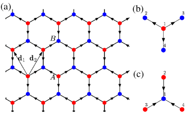
Figure 1: (a) Lattice structure of the model. The arrow indicates the sign of the hopping terms. (b,c) The ordering of the four operators in $g_{1}$ and $g_{2}$ terms, respectively.

The noninteracting model with $g_{1}=g_{2}=0$ exhibits a unique ground state with linearly dispersing single particle excitations near the $\pm\mathbf{K}$ corners of the hexagonal Brillouin zone, analogous to graphene [Castro Neto et al., 2009]. Unlike in graphene and in the previously studied Majorana-Hubbard models [Raghu et al., 2008; Rahmani et al., 2015a, b; Milsted et al., 2015; O’Brien and Fendley, 2018; Zhu and Franz, 2016; Affleck et al., 2017], where weak interactions initially do not change the nature of such a state, we find dramatic effects induced by ${\cal H}_{\mathrm{int}}$ that occur already at infinitesimal coupling strength. Our results are summarized in Fig. 2(a) which shows the phase diagram of the interacting model at weak to intermediate coupling. Except for the line $g_{2}=-g_{1}$ interactions give rise to a gap in the excitation spectrum. As explained below in the two quadrants with $g_{1}g_{2}>0$ the system can be characterized as a Majorana Chern insulator with Chern number $\tilde{{\cal C}}=-{\rm sgn}(g_{1})$ and topologically protected chiral edge modes, Fig. 2(b). This phase belongs to the class D of the Altland-Zirnbauer classification [Chiu et al., 2016]. In the other two quadrants one obtains a Majorana metal with topologically protected antichiral edge modes [Colomés and Franz, 2018] illustrated in Fig. 2(c). At stronger coupling ($g_{1},g_{2}\gtrsim 5t$) our exact diagonalization (ED) numerics suggests a transition to a strongly entangled gapped phase with a doubly degenerate ground state.

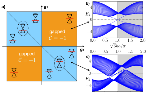
Figure 2: (a) Phase diagram of the interacting Majorana model at weak coupling. MF Hamiltonian Eq. (7) on a strip with the zig-zag boundary (with $\tau_{1}=\pm 0.1,\ \tau_{2}=-0.15$) is used to illustrate the energy spectra in the gapped Majorana Chern insulator phase (b) and the gapless Majorana metal phase (c).

II Symmetries

In addition to discrete translations and ${2\pi\over 3}$ rotations the non-interacting model is invariant under inversion ${\cal P}$ and two reflections ${\cal R}_{1}$ and ${\cal R}_{2}$ indicated in Fig. 3(a). As explained in Appendix A some of these operations must be supplemented by an appropriate Z₂ gauge transformation, which we henceforth denote by ${\cal A}$, in order to become symmetries. It is easy to deduce that ${\cal H}_{\mathrm{int}}$ respects ${\cal P}{\cal A}$ if $g_{1}=g_{2}$ and respects ${\cal R}_{2}{\cal A}$ if $g_{1}=-g_{2}$. Under ${\cal R}_{1}$ the Hamiltonian ${\cal H}(t,g_{1},g_{2})$ maps onto ${\cal H}(t,-g_{1},-g_{2})$. In addition ${\cal H}_{0}$ is invariant under antiunitary time-reversal symmetry $\tilde{{\cal T}}$ which maps $(\alpha_{j},\beta_{j})\to(\alpha_{j},-\beta_{j})$ and $i\to-i$. However, ${\cal H}_{\rm int}$ breaks $\tilde{{\cal T}}$ for any nonzero $g_{1}$, $g_{2}$.

If the Majorana fermions are realized in vortices of the Fu-Kane superconductor then, based on the above analysis, we have $g_{1}=g_{2}$ if the lattice is composed of vortices only, but $g_{1}=-g_{2}$ if sublattice A has vortices and sublattice B antivortices (or vice versa). This is because both ${\cal P}$ and ${\cal R}_{2}$ interchange the sublattices and inversion preserves vorticity while reflection maps vortex onto an antivortex. If the honeycomb lattice becomes distorted such that it no longer respects ${\cal P}$ and ${\cal R}_{2}$, then in general there will be no constraint on $g_{1}$ and $g_{2}$. In the following we analyze the model for arbitrary coupling constants but pay particular attention to the high-symmetry cases discussed above.

III Low-energy theory

It is instructive to examine the low-energy effective theory constructed by expanding the Majorana fields around the two nodal points at $\pm\mathbf{K}$ (see Appendix B for details). One thus obtains

$${\cal H}_{0}\simeq-v\int\mathrm{d}^{2}r\sum_{\sigma=\pm}\sigma\left(\alpha_{\sigma}\partial_{\sigma}\beta_{\bar{\sigma}}+\beta_{\bar{\sigma}}\partial_{\sigma}\alpha_{\sigma}\right),$$ (3)

where $(\alpha_{\pm},\beta_{\pm})$ are the long-wavelength components of the Majorana fields near points $\pm\mathbf{K}$, ${\bar{\sigma}}=-\sigma$, $v=3ta$ is the characteristic velocity, $a$ denotes the lattice constant, and $\partial_{\pm}=(\partial_{x}\pm i\partial_{y})$. Similarly we find

$${\cal H}_{\rm int}\simeq{24\sqrt{3}}a\int d^{2}r\sum_{\sigma=\pm}\bigl{[}g_{1} \beta_{\sigma}\beta_{\bar{\sigma}}(\alpha_{\sigma}\partial_{\sigma}\beta_{\bar{\sigma}})$$

$$+g_{2}\alpha_{\bar{\sigma}}\alpha_{\sigma}(\beta_{\bar{\sigma}}\partial_{\sigma}\alpha_{\sigma})\bigr{]}.$$

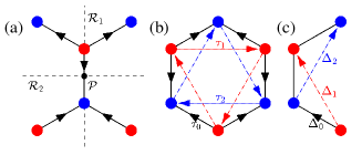
Figure 3: (a) Reflection symmetry $\mathcal{R}_{1,2}$ and inversion symmetry $\mathcal{P}$. (b) The sign convention of the MF Hamiltonian. (c) The definition of the order parameters $\Delta_{a}$.

As in Ref. Affleck et al., 2017 standard renormalization group scaling arguments indicate that interactions are irrelevant in the low-energy theory. The Majorana fields have scaling dimension 1 which gives ${\cal H}_{\rm int}$ dimension 5. The marginal dimension in (2+1)D theory is 3 so the interactions are strongly irrelevant. Naively, one would thus expect the system to remain gapless for weak interactions. We find, however, that this is not the case for the problem at hand due to the special structure of the interaction Hamiltonian (III). We notice that terms in brackets in Eq. (III) coincide with those forming the kinetic part ${\cal H}_{0}$. Clearly terms present in ${\cal H}_{0}$ must have a nonzero vacuum expectation value $\langle\alpha_{\sigma}\partial_{\sigma}\beta_{\bar{\sigma}}\rangle\neq 0$ and $\langle\beta_{\bar{\sigma}}\partial_{\sigma}\alpha_{\sigma}\rangle\neq 0$, and it is easy to see that these expectation values will act as mass terms when inserted into ${\cal H}_{\rm int}$.

If we denote the above expectation values by $m$ then by symmetry we expect $\langle\alpha_{\sigma}\partial_{\sigma}\beta_{\bar{\sigma}}\rangle=\langle\beta_{\bar{\sigma}}\partial_{\sigma}\alpha_{\sigma}\rangle=\sigma m$. Replacing the relevant terms in ${\cal H}_{\rm int}$ by their expectation values and neglecting fluctuations the full low-energy Hamiltonian becomes

$${\cal H}\approx-\int\mathrm{d}^{2}r\sum_{\sigma=\pm}\sigma\Psi^{\dagger}_{\sigma}\pmatrix{-}g_{2}M&-v\partial_{\bar{\sigma}}\\ v\partial_{\sigma}g_{1}M\Psi_{\sigma},$$ (5)

where $\Psi_{\sigma}=(\alpha_{\sigma},\beta_{\sigma})^{T}$ and $M=24\sqrt{3}am$. Assuming translation invariance the spectrum of ${\cal H}$ is easily obtained by passing to the momentum representation,

$$E_{k,\sigma}={1\over 2}\sigma M(g_{1}-g_{2})\pm\sigma\sqrt{v^{2}k^{2}+{1\over 4}M^{2}(g_{1}+g_{2})^{2}},$$ (6)

where $k=(k_{x}^{2}+k_{y}^{2})^{1/2}$. We observe that interactions produce a gap in the Majorana excitation spectrum except when $g_{2}=-g_{1}$. In addition, unequal interaction strengths $g_{1}\neq g_{2}$ cause an offset in energy between two inequivalent nodal points $\pm\mathbf{K}$. These considerations lead to the weak-coupling phase diagram outlined in Fig. 2(a).

When interpreting Eq. (6) one must keep in mind that Majorana fermions carry half the degrees of freedom of ordinary complex fermions. Because of this only half of the states implied by $E_{k,\sigma}$ are physical. Customarily one can either focus on positive-energy states at all momenta or, equivalently take all energies but restrict to one-half of the Brillouin zone. In illustrating various phases of the model we take the latter point of view and focus on states near $+\mathbf{K}$.

IV Mean-field theory

The low-energy analysis suggests that at weak coupling accurate results can be obtained using mean-field (MF) decoupling of the lattice interaction terms Eq. (1). As an example we may approximate $\alpha_{i}\beta_{j}\beta_{k}\beta_{l}\to\langle\alpha_{i}\beta_{j}\rangle\beta_{k}\beta_{l}$ where the expectation value lives on the nearest neighbor bond (terms already present in ${\cal H}_{0}$) and the operator product $\beta_{k}\beta_{l}$ describes coupling between next nearest neighbors. This motivates study of the MF Hamiltonian with first and second neighbor hoppings

$${\cal H}_{\mathrm{MF}}=i\sum_{\langle ij\rangle}\eta_{ij}\tau_{0}\alpha_{i}\beta_{j}+i\sum_{\langle\langle ij\rangle\rangle}\eta_{ij}(\tau_{1}\alpha_{i}\alpha_{j}+\tau_{2}\beta_{i}\beta_{j}),$$ (7)

with the signs specified in Fig. 3(b). We expect the eigenstates of ${\cal H}_{\mathrm{MF}}$ to capture the essential physics of the problem at weak coupling and in the following we employ them as variational wave functions for the full Hamiltonian (1), parametrized by $\{\tau_{a}\}$.

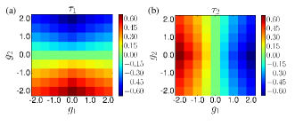
Figure 4: Self-consistent solution of the MF equations (12).

Before linking ${\cal H}_{\mathrm{MF}}$ to the interacting Hamiltonian, it is useful to understand its properties. In $k$ space, the Hamiltonian reads

$${\cal H}_{\mathrm{MF}}=\sum_{\mathbf{k}}\Psi_{\mathbf{k}}^{\dagger}\pmatrix{4}\tau_{1}D_{2}(\mathbf{k})&2\tau_{0}D_{1}(\mathbf{k})\\ 2\tau_{0}D_{1}^{*}(\mathbf{k})-4\tau_{2}D_{2}(\mathbf{k})\Psi_{\mathbf{k}}+E_{0},$$ (8)

where $\Psi_{\mathbf{k}}=(\alpha_{\mathbf{k}},\beta_{\mathbf{k}})^{T}$,

$$\split D_{1}(\mathbf{k})&=i(1+\mathrm{e}^{i\mathbf{k}\cdot\mathbf{d}_{1}}+\mathrm{e}^{i\mathbf{k}\cdot\mathbf{d}_{2}})\\ D_{2}(\mathbf{k})=-\sin\mathbf{d}_{1}\cdot\mathbf{k}+\sin\mathbf{d}_{2}\cdot\mathbf{k}+\sin(\mathbf{d}_{1}-\mathbf{d}_{2})\cdot\mathbf{k}$$ (9)

and $E_{0}=2(\tau_{2}-\tau_{1})\sum_{\mathbf{k}}D_{2}(\mathbf{k})$. The MF spectrum is

$$E_{\mathbf{k},\pm}=2(\tau_{1}-\tau_{2})D_{2}\pm 2\epsilon_{\mathbf{k}},$$ (10)

with $\epsilon_{\mathbf{k}}=\sqrt{\tau_{0}^{2}|D_{1}|^{2}+(\tau_{1}+\tau_{2})^{2}D_{2}^{2}}$.

As usual, the fact that $\alpha_{-\mathbf{k}}=\alpha_{\mathbf{k}}^{\dagger}$ and $\beta_{-\mathbf{k}}=\beta_{\mathbf{k}}^{\dagger}$ introduces a redundancy in the $k$ space, and we restrict ourselves to half of the BZ. We also take $\tau_{0}=1$ without loss of generality. The phase diagram of the model is then the same as in Fig. 2(a) with $(g_{1},g_{2})$ replaced with $(-\tau_{2},-\tau_{1})$.

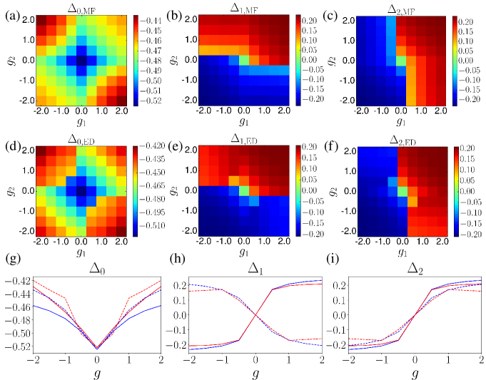
Figure 5: Order parameters $\Delta_{a}$ (a)-(c) from MF calculations and (d)-(f) from ED using a cluster of 32 lattice sites with periodic boundary conditions. (g)-(i) Quantitative comparison between MF (blue) and ED (red) results, with solid line $g_{1}=g_{2}=g$ and dash line $g_{1}=-g_{2}=g$.

The MF Hamiltonian above resembles the Haldane model [Haldane, 1988]; thus we expect topologically protected edge modes in a system with boundaries. In fact, we can readily calculate the Chern number from the bulk solutions with the caveat that the redundancy of the $k$-space Hamiltonian implies a Majorana edge mode. For the insulating phases, $\tau_{1}\tau_{2}>0$, the Chern number is

$$\widetilde{\mathcal{C}}=\mathrm{sgn}(\tau_{1})=\mathrm{sgn}(\tau_{2}).$$ (11)

We calculate numerically the energy spectrum of the system placed on a strip with a zig-zag boundary along the $x$ direction. The energy spectra for $\tau_{1}=\pm 0.1,$ and $\tau_{2}=-0.15$ are shown in Figs. 2(b) and 2(c). The edge modes are clearly present in both cases. They are chiral for $\tau_{1}\tau_{2}>0$ and antichiral for $\tau_{1}\tau_{2}<0$. Chiral edge modes propagate in the opposite direction on two opposite edges and are protected by the bulk invariant $\tilde{\cal C}$. Antichiral edge modes propagate in the same direction and are protected, to a lesser degree, by their real-space segregation from the bulk modes [Colomés and Franz, 2018].

Now we use the ground state $|\Psi_{\mathrm{MF}}\rangle$ of the MF Hamiltonian as a variational ansatz to analyze the interacting problem. As outlined in Appendix C, the requirement that $\langle\Psi_{\mathrm{MF}}|{\cal H}|\Psi_{\mathrm{MF}}\rangle$ is minimized gives the MF equations for parameters $\tau_{a}$,

$$\split\tau_{0}&=t+g_{1}\Delta_{2}+g_{2}\Delta_{1},\\ \tau_{1}=g_{2}\Delta_{0},\\ \tau_{2}=g_{1}\Delta_{0},$$ (12)

where the order parameters $\Delta_{0}=i\langle\alpha_{1}\beta_{2}\rangle$, $\Delta_{1}=i\langle\alpha_{1}\alpha_{2}\rangle$, and $\Delta_{2}=i\langle\beta_{1}\beta_{2}\rangle$ are defined on bonds specified in Fig. 3(c). The expectation values are taken with respect to $|\Psi_{\mathrm{MF}}\rangle$ and are functions of the variational parameters $\{\tau_{a}\}$. They can be expressed as momentum space sums involving $D_{1}(\mathbf{k})$, $D_{2}(\mathbf{k})$, and $\epsilon_{\mathbf{k}}$, which we give in Appendix C.

We solve the MF equations (12) by numerical iteration, and the results are summarized in Figs. 4 and 5. We find that $\Delta_{0}\simeq-0.5t$ when $g_{1}=g_{2}=0$ and changes very little with interactions [Fig. 5(a]. Equations (12) then imply that $\tau_{1}$ and $\tau_{2}$ become nonzero for arbitrarily weak interaction strengths $g_{1,2}$. As a result, we see that an effective second neighbor hopping is introduced by an infinitesimal interaction strength whereby the system becomes gapped. MF theory is therefore in full agreement with our field-theoretic low-energy analysis.

The above instability of the gapless phase is to be contrasted with the results on the square lattice [Affleck et al., 2017], where interaction strength $|g|\simeq 0.9t$ is required for the system to enter a gapped phase. This contrasting behavior can be understood from symmetry considerations. As in graphene the gapless spectrum near Dirac points is protected here by a combination of inversion ${\cal P}$ and time reversal ${\tilde{\cal T}}$. While the full interacting Hamiltonian in Ref.  Affleck et al., 2017 respects these symmetries, ${\tilde{\cal T}}$ is explicitly broken by the interaction term on the honeycomb lattice.

V Exact diagonalization and strong coupling limit

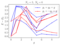
Figure 6: Lowest many-body energy levels of ${\cal H}$ computed using ED for different values of $g$.

We perform exact numerical diagonalization of the full interacting lattice model on clusters with up to $N=32$ sites to ascertain the validity of the MF results discussed above and to gain insights into the strong coupling limit. Figures 5(d)-5(f) show our ED results for order parameters $\Delta_{a}$ compared to the results of the MF analysis. At weak to intermediate coupling ($|g_{1}|,|g_{2}|\lesssim 2t$) we see that unbiased ED approach lends full support to our MF results. At stronger coupling the two approaches begin to diverge which suggests a breakdown of the MF theory in this limit.

We also calculate the lowest many-body energies using ED as a function of $g_{1}=\pm g_{2}=g$; see Fig. 6. Although the detailed behavior of the energy levels depends on the system geometry and size, the results suggest that a phase transition occurs near $g\sim 5t$. Above the transition the pattern of energy levels shown in Fig. 7 is suggestive of a doubly degenerate ground state and an excitation gap that grows linearly with $g$.

As a final topic, we briefly discuss the physics of the model at large $g$. Analytical progress in this limit is hampered by the fact that there is no obvious solution to the problem when $t=0$. Since the $g_{1}$ and $g_{2}$ terms in ${\cal H}_{\mathrm{int}}$ are seen to mutually commute the problem in this limit separates into two commuting Hamiltonians that can be treated independently. Nevertheless, these still remain difficult problems with no obvious solution.

For $t=0$, it is possible to map ${\cal H}_{\rm int}$ onto a local spin-${1\over 2}$ model on a triangular lattice using the Jordan-Wigner transformation. A set of Majorana operators ${\alpha_{j},\beta_{j}}$ can be mapped onto a set spin-${1\over 2}$ operators $\mathbf{\sigma}_{j}$ as

$$\alpha_{i}=\prod_{k<i}(-\sigma_{k}^{z})\sigma_{i}^{x},\ \ \ \beta_{i}=\prod_{k<i}(-\sigma_{k}^{z})\sigma_{i}^{y}.$$ (13)

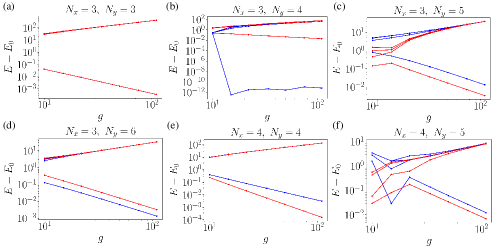
Figure 7: Lowest many-body energy levels in the large $g$ limit, where $g_{1}=(-)g_{2}=g$ for the blue (red) curve as in Fig. 6.

For a generic local fermion Hamiltonian in dimension greater than 1, however, the spin Hamiltonian might contain non-local terms due to the products of $\sigma_{k}^{z}$ operators that appear in Eq. (13). Fortunately, in the present case for $t=0$, the Hamiltonian remains strictly local if we choose the path shown in Fig. 8(a) to order the sites. We thus get

$$\split&{\cal H}_{\Ydown}:\ \ g_{1}\alpha_{k}\beta_{i}\beta_{j}\beta_{k}=g_{1}\sigma_{k}^{z}\sigma_{i}^{x}\sigma_{j}^{y},\\ {\cal H}_{\Yup}:\ \ g_{2}\beta_{j}\alpha_{j}\alpha_{k}\alpha_{l}=g_{2}\sigma_{j}^{z}\sigma_{k}^{y}\sigma_{l}^{x},$$ (14)

and the Hamiltonian is

$${\cal H}_{\rm spin}=\left(g_{1}\sum_{\nabla}+g_{2}\sum_{\Delta}\right)\sigma_{1}^{z}\sigma_{2}^{x}\sigma_{3}^{y},$$ (15)

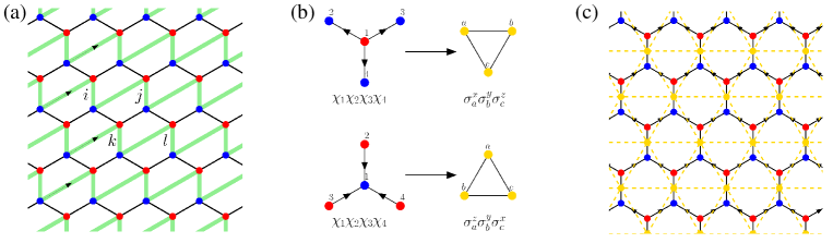
Figure 8: Jordan-Wigner transformation. (a) The path used to define the Jordan-Wigner transformation Eq. (13). (b) Each four-Majorana interaction term maps onto a three-spin interaction. (c) The resulting triangular lattice spin model.

where the spins can be thought of as living on the midpoints of all vertical bonds of the original honeycomb lattice, and are arranged on each triangle as indicated in Fig. 8(b). The spin system thus forms a triangular lattice, Fig. 8(c).

This is a highly frustrated Hamiltonian: while it is possible to minimize the product of three spin operators on each of the triangles in isolation it is not possible to do so for two triangles sharing a single vertex. We thus conjecture that at strong coupling the MF state discussed in the previous sections will give way to a highly entangled strong coupling phase that can be viewed in the spin representation as a spin liquid. The spin model (15) shares some obvious similarities with the celebrated Kitaev honeycomb lattice model [Kitaev, 2006], but as far as we can tell it does not have an exact solution.

ED calculations on small clusters at large $g$ indicate a featureless ground state with $\langle\alpha_{1}\beta_{2}\beta_{3}\beta_{4}\rangle=\langle\beta_{1}\alpha_{2}\alpha_{3}\alpha_{4}\rangle\simeq\pm 1/2$ on each plaquette (the sign depends on whether $g_{1}=g_{2}$ or $g_{1}=-g_{2}$). Two-fermion expectation values on first and second neighbors are likewise featureless and in addition small compared to unity. No obvious pattern of symmetry breaking is revealed by our investigation. Collectively these results suggest a nontrivial, highly entangled featureless state in the strong coupling limit which can be possibly viewed as a spin liquid when represented through the spin Hamiltonian (15). More work is clearly necessary to determine the properties of this state.

VI Conclusion

Majorana-Hubbard model on the honeycomb lattice exhibits interesting interaction-driven topological phases that occur already at weak coupling. This is unlike other Majorana-Hubbard models previously discussed in the literature [Raghu et al., 2008; Rahmani et al., 2015a, b; Milsted et al., 2015; O’Brien and Fendley, 2018; Zhu and Franz, 2016; Affleck et al., 2017]. The key distinction here is that the most local interaction term on the honeycomb lattice explicitly breaks the time-reversal symmetry ${\tilde{\cal T}}$ which normally acts to protect the gapless nature of the excitation spectrum.

The model may be realized at a proximitized surface of a 3D topological insulator [Fu and Kane, 2008; Chiu et al., 2015] if a vortex lattice with the honeycomb geometry can be stabilized. This could be achieved for instance by engineering such a surface with an array of pinning sites designed to bind vortices into the honeycomb lattice arrangement [Baert et al., 1995; Harada et al., 1996].

A related Majorana model on the honeycomb lattice with six-fermion interactions was introduced in Ref. Vijay et al., 2015 together with a proposal for an experimental realization at a topological insulator surface. In this setting our model becomes relevant when the Majorana mode wavefunctions have large overlaps. The the hopping parameter $t$ relative to the interaction parameter $g$ can be tuned e.g. by shifting the chemical potential of the topological insulator as discussed in Ref. Rahmani et al., 2015b. Our predictions for interaction-driven topological phases can be tested by spectroscopic measurements using a scanning tunneling microscope, which is capable of locally distinguishing between gapped bulk and gapless edges of the system.

Acknowledgments.– We thank Ian Affleck, Oğuzhan Can, Étienne Lantagne-Hurtubise and Tarun Tummuru for helpful discussions. The work described in this article was supported by NSERC and CIfAR.

Appendix A LATTICE MODEL SYMMETRIES

We examine the symmetries of ${\cal H}_{0}$ and ${\cal H}_{\mathrm{int}}$ at the same time. In both Hamiltonians we have discrete translational symmetry and ${2\pi\over 3}$ rotational symmetry. A general honeycomb lattice model with these symmetries can in addition possess an inversion and two different reflection symmetries; see Fig. 3(a). It can be easily checked that the reflection symmetry with regard to the hexagon diagonal, $\mathcal{R}_{1}$, is respected by the noninteracting model, but broken by the interactions. Indeed, under $\mathcal{R}_{1}$, ${\cal H}(t,g_{1},g_{2})$ maps to ${\cal H}(t,-g_{1},-g_{2})$.

Under inversion $\mathcal{P}$ sublattices interchange $A\leftrightarrow B$ and therefore $\alpha_{j}\leftrightarrow\beta_{j}$. In order to compensate for the minus sign in ${\cal H}_{0}$, we introduce a transformation $\mathcal{A}:\alpha\rightarrow-\alpha$, which amounts to a Z₂ gauge transformation and thus does not change the physics. One can check easily that $\mathcal{PA}$ is preserved if and only if $g_{1}=g_{2}$ in the interacting case. Similar results hold for the other reflection $\mathcal{R}_{2}$, where $\mathcal{R}_{2}\mathcal{A}$ is preserved if and only if $g_{1}=-g_{2}$. For general $g_{1,2}$, $\mathcal{P}\mathcal{A}$ and $\mathcal{R}_{2}\mathcal{A}$ map ${\cal H}(t,g_{1},g_{2})$ to ${\cal H}(t,g_{2},g_{1})$ and ${\cal H}(t,-g_{2},-g_{1})$, respectively. Thus we are allowed to focus only on the case $g_{1}\geq|g_{2}|$, and the behavior of the system in the remaining regions of the phase diagram can be obtained from symmetry considerations. For example, the energy spectrum is the same for ${\cal H}(t,g_{1},g_{2})$ and ${\cal H}(t,-g_{2},-g_{1})$, while the Chern number acquires a minus sign.

Time reversal symmetry (TRS) is more subtle. Physically, we expect Majorana modes to appear in the presence of the magnetic field; thus physical TRS is broken from the very beginning. Nevertheless ${\cal H}_{0}$ is invariant under antiunitary symmetry $\tilde{{\cal T}}$: $(\alpha_{j},\beta_{j})\to(\alpha_{j},-\beta_{j})$ and $i\to-i$ which acts, effectively, as a time reversal with $\tilde{{\cal T}}^{2}=+1$. The interaction term breaks this symmetry as ${\cal H}(t,g_{1},g_{2})$ maps to ${\cal H}(t,-g_{1},-g_{2})$ under $\tilde{{\cal T}}$. It follows that a combined operation $\tilde{{\cal T}}\mathcal{R}_{1}$ is a symmetry of the full Hamiltonian for any $g_{1}$, $g_{2}$. The action of various symmetries is summarized in Table 1.

Vortices and antivortices remain the same under inversion (with an immaterial minus sign), but map onto each other under reflections. Thus we expect $\mathcal{P}$ to be relevant for a lattice of (anti-)vortices, while $\mathcal{R}_{1,2}$ are respected by a bipartite lattice of vortices (antivortices) occupying sublattice A (B). This motivates our exploration of the phase diagram for arbitrary $g_{1,2}$ with special focus on two lines $g_{2}=\pm g_{1}$.

Symmetry	translation	$2\pi/3$ rotation
Condition	none
Symmetry	$\mathcal{R}_{1},\mathcal{T}$	$\mathcal{P}\mathcal{A}$	$\mathcal{R}_{2}\mathcal{A}$
Condition	$g_{1}=g_{2}=0$	$g_{1}=g_{2}$	$g_{1}=-g_{2}$

Table 1: The symmetries of the model, with definitions in the text.

Appendix B LOW-ENERGY FIELD THEORY

The non-interacting Hamiltonian ${\cal H}_{0}$ given in Eq. (1) of the main text can be analyzed by introducing momentum-space Majorana operators

$$\pmatrix{\alpha}_{j}\\ \beta_{j}=\sqrt{\frac{2}{N}}\sum_{\mathbf{k}}\mathrm{e}^{i{\mathbf{r}}_{j}\cdot\mathbf{k}}\pmatrix{\alpha}_{\mathbf{k}}\\ \beta_{\mathbf{k}},$$ (16)

where $\mathbf{r}_{j}$ labels the unit cell. It is important to note that the Fourier transform introduces a redundancy: because

$$(\alpha_{\mathbf{k}}^{\dagger},\beta_{\mathbf{k}}^{\dagger})=(\alpha_{-\mathbf{k}},\beta_{-\mathbf{k}})$$ (17)

the Fourier-space operators are no longer self-conjugate. One can deal with the redundancy in two ways: (i) either view $(\alpha_{\mathbf{k}},\beta_{\mathbf{k}})$ as independent across the entire BZ but only consider positive energy eigenstates, or (ii) restrict $\mathbf{k}$ to one half of the BZ and consider all the states.

In the momentum space the Hamiltonian can be written as ${\cal H}_{0}=\sum^{\prime}_{\mathbf{k}}\Psi_{\mathbf{k}}^{\dagger}h_{0}(\mathbf{k})\Psi_{\mathbf{k}}$ where $\Psi_{\mathbf{k}}=(\alpha_{\mathbf{k}},\beta_{\mathbf{k}})^{T}$, the prime denotes summation over half BZ and

$$h_{0}(\mathbf{k})=2t\pmatrix{0}&D_{1}(\mathbf{k})\\ D_{1}^{*}(\mathbf{k})0,$$ (18)

with $D_{1}(\mathbf{k})=i(1+\mathrm{e}^{i\mathbf{k}\cdot\mathbf{d}_{1}}+\mathrm{e}^{i\mathbf{k}\cdot\mathbf{d}_{2}})$. Here $\mathbf{d}_{j}$ are the primitive vectors of the Bravais lattice given by $\mathbf{d}_{1,2}=(\mp\frac{\sqrt{3}}{2}a,\frac{3}{2}a)$. The diagonalization is straightforward and we have

$$E_{\mathbf{k},\pm}=\pm 2t|1+\mathrm{e}^{i\mathbf{k}\cdot\mathbf{d}_{1}}+\mathrm{e}^{i\mathbf{k}\cdot\mathbf{d}_{2}}|.$$ (19)

The energy spectrum is identical to that of the Dirac fermion model on the honeycomb lattice familiar from graphene and exhibits nodal points at $\pm\mathbf{K}$ with $\mathbf{K}=(\frac{2\pi}{3\sqrt{3}a},\frac{2\pi}{3a})$. Expansion of the Hamiltonian (18) near $+\mathbf{K}$, writing $\mathbf{k}=\mathbf{K}+\mathbf{q}$ and assuming $|\mathbf{q}|$ small, gives a massless Dirac Hamiltonian

$$h_{0}(\mathbf{k})\simeq v\pmatrix{0}&q_{y}+iq_{x}\\ q_{y}-iq_{x}0,$$ (20)

with velocity $v=3ta$ and the spectrum $E_{\mathbf{q}}\simeq\pm v|\mathbf{q}|$.

To derive the low-energy continuum theory we approximate the Majorana fields by expanding close to the two nodal points,

$$\split\alpha(\mathbf{r})&\simeq 2(e^{i\mathbf{K}\cdot\mathbf{r}}\alpha_{+}(\mathbf{r})+e^{-i\mathbf{K}\cdot\mathbf{r}}\alpha_{-}(\mathbf{r})),\\ \beta(\mathbf{r})\simeq 2(e^{i\mathbf{K}\cdot\mathbf{r}}\beta_{+}(\mathbf{r})+e^{-i\mathbf{K}\cdot\mathbf{r}}\beta_{-}(\mathbf{r})),$$ (21)

where $(\alpha_{\sigma},\beta_{\sigma})$ with $\sigma=\pm$ are slowly varying on the lattice scale and the normalization is chosen for later convenience. Substituting into the Hamiltonian we get

$$\split{\cal H}_{0}&\simeq 4it\int\mathrm{d}r\left[e^{i\mathbf{K}\cdot\mathbf{r}}\alpha_{+}(\mathbf{r})+e^{-i\mathbf{K}\cdot\mathbf{r}}\alpha_{-}(\mathbf{r})\right]\\ \quad\times\bigl{[}e^{i\mathbf{K}\cdot\mathbf{r}}\beta_{+}(\mathbf{r})+e^{-i\mathbf{K}\cdot\mathbf{r}}\beta_{-}(\mathbf{r})\\ \quad+e^{i\mathbf{K}\cdot(\mathbf{r}+\mathbf{d}_{1})}\beta_{+}(\mathbf{r}+\mathbf{d}_{1})+e^{-i\mathbf{K}\cdot(\mathbf{r}+\mathbf{d}_{1})}\beta_{-}(\mathbf{r}+\mathbf{d}_{1})\\ \quad+e^{i\mathbf{K}\cdot(\mathbf{r}+\mathbf{d}_{2})}\beta_{+}(\mathbf{r}+\mathbf{d}_{2})+e^{-i\mathbf{K}\cdot(\mathbf{r}+\mathbf{d}_{2})}\beta_{-}(\mathbf{r}+\mathbf{d}_{2})\bigr{]}.$$ (22)

Now we expand the fields to leading order in $\mathbf{d}_{j}$, e.g. $\beta_{\sigma}(\mathbf{r}+\mathbf{d}_{j})\simeq\beta_{\sigma}(\mathbf{r})+\mathbf{d}_{j}\cdot\nabla\beta_{\sigma}(\mathbf{r})$, and retain only the slowly-varying terms (i.e. those not containing $e^{\pm i\mathbf{K}\cdot\mathbf{r}}$ factors). We thus obtain the leading low-energy free Hamiltonian

$${\cal H}_{0}\simeq-6ta\int\mathrm{d}r\big{[}\alpha_{-}(-\partial_{x}+i\partial_{y})\beta_{+}+\alpha_{+}(\partial_{x}+i\partial_{y})\beta_{-}\big{]}.$$ (23)

Integrating by parts then leads to Eq. (3) of the main text.

It is also possible to express the kinetic term in the form of a Dirac Hamiltonian,

$${\cal H}_{0}\simeq-iv\int\mathrm{d}r\sum_{\sigma=\pm}\Psi_{\sigma}^{\dagger}\left(\sigma\tau^{y}\partial_{x}+\tau^{x}\partial_{y}\right)\Psi_{\sigma},$$ (24)

where $\tau^{a}$ are Pauli matrices, $\Psi_{\sigma}=(\alpha_{\sigma},\beta_{\sigma})^{T}$ and $\Psi_{\sigma}^{\dagger}=(\alpha_{\bar{\sigma}},\beta_{\bar{\sigma}})$. One could go one step further and write down the Lagrangian of the theory which shows explicitly the emergent low-energy Lorentz invariance, expected from a model defined on the honeycomb lattice.

Analogous procedure can be applied to ${\cal H}_{\rm int}$ and leads to the low-energy expansion given in Eq. (4). It is to be noted that unlike the effective low-energy theory on the square lattice (where the interaction term contains no derivatives) here one derivative is mandated because of the lattice structure of the interaction term. It comprises either three $\alpha$ operators and one $\beta$ or vice versa. It is easy to see that there is no way in this case to write a non-derivative four-fermion term in the low-energy expansion. One can of course have $\alpha_{+}\alpha_{-}\beta_{+}\beta_{-}$ but this corresponds to a longer-range interaction term in the original lattice Hamiltonian, comprising two A sites and two B sites of the honeycomb lattice, which will be weaker on general grounds and we are therefore neglecting it here.

Appendix C DERIVATION OF THE MEAN-FIELD GAP EQUATIONS

To begin we introduce the order parameters

$$\split&\Delta_{0}=i\langle\alpha_{i,1}\beta_{i,2}\rangle,\\ \Delta_{1}=i\langle\alpha_{i,1}\alpha_{i,2}\rangle,\\ \Delta_{2}=i\langle\beta_{i,1}\beta_{i,2}\rangle,$$ (25)

assuming translational invariance and signs illustrated in Fig. 3(c). Using these we can write the mean field ground state energy as

$$E_{\mathrm{MF}}=\langle\Psi_{\mathrm{MF}}|{\cal H}_{\mathrm{MF}}|\Psi_{\mathrm{MF}}\rangle=3N\sum_{a=0}^{2}\tau_{a}\Delta_{a},$$ (26)

and it holds that

$$\Delta_{a}=\frac{1}{3N}\frac{\partial E_{\mathrm{MF}}}{\partial\tau_{a}},$$ (27)

by the Hellmann-Feynman theorem. Using Eq.  (10), we can explicitly perform the derivatives and get a set of equations

$$\split\Delta_{0}&=\frac{2\tau_{0}}{3N}\Big{(}\sum_{\mathbf{k}:+}\frac{|D_{1}|^{2}}{\epsilon_{\mathbf{k}}}-\sum_{\mathbf{k}:-}\frac{|D_{1}|^{2}}{\epsilon_{\mathbf{k}}}\Big{)},\\ \Delta_{1}=\frac{2}{3N}\Big{(}\sum_{\mathbf{k}:+}\Big{(}D_{2}+\frac{(\tau_{1}+\tau_{2})D_{2}^{2}}{\epsilon_{\mathbf{k}}}\Big{)}\\ +\sum_{\mathbf{k}:-}\Big{(}D_{2}-\frac{(\tau_{1}+\tau_{2})D_{2}^{2}}{\epsilon_{\mathbf{k}}}\Big{)}-\sum_{\mathbf{k}}D_{2}\Big{)},\\ \Delta_{2}=\frac{2}{3N}\Big{(}\sum_{\mathbf{k}:+}\Big{(}-D_{2}+\frac{(\tau_{1}+\tau_{2})D_{2}^{2}}{\epsilon_{\mathbf{k}}}\Big{)}\\ +\sum_{\mathbf{k}:-}\Big{(}-D_{2}-\frac{(\tau_{1}+\tau_{2})D_{2}^{2}}{\epsilon_{\mathbf{k}}}\Big{)}+\sum_{\mathbf{k}}D_{2}\Big{)},$$ (28)

where $\sum_{\mathbf{k}:\pm}$ denotes summation over the occupied (i.e. negative-energy) states in the upper (+) or lower ($-$) band.

The MF energy of the full interacting model can also be easily written down in terms of $\{\Delta_{a}\}$,

$$\langle{\cal H}\rangle=\langle\Psi_{\mathrm{MF}}|{\cal H}_{0}+{\cal H}_{\mathrm{int}}|\Psi_{\mathrm{MF}}\rangle=3N\Delta_{0}(t+g_{1}\Delta_{2}+g_{2}\Delta_{1}).$$ (29)

Now we can get the gap equations by minimizing the energy with respect to variational parameters $\{\tau_{a}\}$,

$$\frac{\partial\langle{\cal H}\rangle}{\partial\tau_{a}}=0,$$ (30)

or more explicitly

$$\frac{\partial\Delta_{0}}{\partial\tau_{a}}(t+g_{1}\Delta_{2}+g_{2}\Delta_{1})+\Delta_{0}\Big{(}g_{1}\frac{\partial\Delta_{2}}{\partial\tau_{a}}+g_{2}\frac{\partial\Delta_{1}}{\partial\tau_{a}}\Big{)}=0.$$ (31)

We also note a corollary of the Hellmann-Feynman theorem

$$\sum_{a=0}^{2}\tau_{a}\frac{\partial\Delta_{a}}{\partial\tau_{a}}=0.$$ (32)

It is easy to check that the last two equations are solved by variational parameters $\{\tau_{a}\}$ given by Eqs. (12) in the main text and order parameters $\{\Delta_{a}\}$ given by Eq. (28).

References

- Hirsch (1985) J. E. Hirsch, Phys. Rev. B 31, 4403 (1985).
- White et al. (1989) S. R. White, D. J. Scalapino, R. L. Sugar, E. Y. Loh, J. E. Gubernatis, and R. T. Scalettar, Phys. Rev. B 40, 506 (1989).
- Bickers et al. (1989) N. E. Bickers, D. J. Scalapino, and S. R. White, Phys. Rev. Lett. 62, 961 (1989).
- Sorella and Tosatti (1992) S. Sorella and E. Tosatti, EPL (Europhysics Letters) 19, 699 (1992).
- Read and Green (2000) N. Read and D. Green, Phys. Rev. B 61, 10267 (2000).
- Kitaev (2001) A. Y. Kitaev, Physics-Uspekhi 44, 131 (2001).
- Stern (2008) A. Stern, Ann. Phys. 323, 204 (2008).
- Nayak et al. (2008) C. Nayak, S. H. Simon, A. Stern, M. Freedman, and S. Das Sarma, Rev. Mod. Phys. 80, 1083 (2008).
- Fu and Kane (2008) L. Fu and C. L. Kane, Phys. Rev. Lett. 100, 096407 (2008).
- Lutchyn et al. (2010) R. M. Lutchyn, J. D. Sau, and S. Das Sarma, Phys. Rev. Lett. 105, 077001 (2010).
- Oreg et al. (2010) Y. Oreg, G. Refael, and F. von Oppen, Phys. Rev. Lett. 105, 177002 (2010).
- Alicea (2012) J. Alicea, Rep. Prog. Phys. 75, 076501 (2012).
- Beenakker (2013) C. Beenakker, Annu. Rev. Condens. Matter Phys. 4, 113 (2013).
- Elliott and Franz (2015) S. R. Elliott and M. Franz, Rev. Mod. Phys. 87, 137 (2015).
- Mourik et al. (2012) V. Mourik, K. Zuo, S. M. Frolov, S. R. Plissard, E. P. A. M. Bakkers, and L. P. Kouwenhoven, Science 336, 1003 (2012).
- Das et al. (2012) A. Das, Y. Ronen, Y. Most, Y. Oreg, M. Heiblum, and H. Shtrikman, Nat. Phys. 8, 887 (2012).
- Deng et al. (2012) M. T. Deng, C. L. Yu, G. Y. Huang, M. Larsson, P. Caroff, and H. Q. Xu, Nano Lett. 12, 6414 (2012).
- Rokhinson et al. (2012) L. P. Rokhinson, X. Liu, and J. K. Furdyna, Nat. Phys. 8, 795 (2012).
- Finck et al. (2013) A. D. K. Finck, D. J. Van Harlingen, P. K. Mohseni, K. Jung, and X. Li, Phys. Rev. Lett. 110, 126406 (2013).
- Hart et al. (2014) S. Hart, H. Ren, T. Wagner, P. Leubner, M. Mühlbauer, C. Brüne, H. Buhmann, L. W. Molenkamp, and A. Yacoby, Nat. Phys. 10, 638 (2014).
- Nadj-Perge et al. (2014) S. Nadj-Perge, I. K. Drozdov, J. Li, H. Chen, S. Jeon, J. Seo, A. H. MacDonald, B. A. Bernevig, and A. Yazdani, Science 346, 602 (2014).
- Kammhuber et al. (2017) J. Kammhuber, M. C. Cassidy, F. Pei, M. P. Nowak, A. Vuik, Ö. Gül, D. Car, S. R. Plissard, E. P. A. M. Bakkers, M. Wimmer, and L. P. Kouwenhoven, Nat. Commun. 8, 478 (2017).
- He et al. (2017) Q. L. He, L. Pan, A. L. Stern, E. C. Burks, X. Che, G. Yin, J. Wang, B. Lian, Q. Zhou, E. S. Choi, K. Murata, X. Kou, Z. Chen, T. Nie, Q. Shao, Y. Fan, S.-C. Zhang, K. Liu, J. Xia, and K. L. Wang, Science 357, 294 (2017).
- Majorana (1937) E. Majorana, Il Nuovo Cimento (1924-1942) 14, 171 (1937).
- Rahmani et al. (2015a) A. Rahmani, X. Zhu, M. Franz, and I. Affleck, Phys. Rev. Lett. 115, 166401 (2015a).
- Rahmani et al. (2015b) A. Rahmani, X. Zhu, M. Franz, and I. Affleck, Phys. Rev. B 92, 235123 (2015b).
- Milsted et al. (2015) A. Milsted, L. Seabra, I. C. Fulga, C. W. J. Beenakker, and E. Cobanera, Phys. Rev. B 92, 085139 (2015).
- (28) N. Sannomiya and H. Katsura, arXiv:1712.01148 .
- O’Brien and Fendley (2018) E. O’Brien and P. Fendley, Phys. Rev. Lett. 120, 206403 (2018).
- Zhu and Franz (2016) X. Zhu and M. Franz, Phys. Rev. B 93, 195118 (2016).
- Affleck et al. (2017) I. Affleck, A. Rahmani, and D. Pikulin, Phys. Rev. B 96, 125121 (2017).
- Chiu et al. (2015) C.-K. Chiu, D. I. Pikulin, and M. Franz, Phys. Rev. B 91, 165402 (2015).
- Xu et al. (2015) J.-P. Xu, M.-X. Wang, Z. L. Liu, J.-F. Ge, X. Yang, C. Liu, Z. A. Xu, D. Guan, C. L. Gao, D. Qian, Y. Liu, Q.-H. Wang, F.-C. Zhang, Q.-K. Xue, and J.-F. Jia, Phys. Rev. Lett. 114, 017001 (2015).
- Sun et al. (2016) H.-H. Sun, K.-W. Zhang, L.-H. Hu, C. Li, G.-Y. Wang, H.-Y. Ma, Z.-A. Xu, C.-L. Gao, D.-D. Guan, Y.-Y. Li, C. Liu, D. Qian, Y. Zhou, L. Fu, S.-C. Li, F.-C. Zhang, and J.-F. Jia, Phys. Rev. Lett. 116, 257003 (2016).
- Semenoff (1984) G. W. Semenoff, Phys. Rev. Lett. 53, 2449 (1984).
- Haldane (1988) F. D. M. Haldane, Phys. Rev. Lett. 61, 2015 (1988).
- Kane and Mele (2005) C. L. Kane and E. J. Mele, Phys. Rev. Lett. 95, 226801 (2005).
- Geim and Novoselov (2007) A. K. Geim and K. S. Novoselov, Nat. Mater. 6, 183 (2007).
- Castro Neto et al. (2009) A. H. Castro Neto, F. Guinea, N. M. R. Peres, K. S. Novoselov, and A. K. Geim, Rev. Mod. Phys. 81, 109 (2009).
- Cao et al. (2018) Y. Cao, V. Fatemi, S. Fang, K. Watanabe, T. Taniguchi, E. Kaxiras, and P. Jarillo-Herrero, Nature 556, 43 (2018).
- Grosfeld and Stern (2006) E. Grosfeld and A. Stern, Phys. Rev. B 73, 201303 (2006).
- Raghu et al. (2008) S. Raghu, X.-L. Qi, C. Honerkamp, and S.-C. Zhang, Phys. Rev. Lett. 100, 156401 (2008).
- Chiu et al. (2016) C.-K. Chiu, J. C. Y. Teo, A. P. Schnyder, and S. Ryu, Rev. Mod. Phys. 88, 035005 (2016).
- Colomés and Franz (2018) E. Colomés and M. Franz, Phys. Rev. Lett. 120, 086603 (2018).
- Kitaev (2006) A. Kitaev, Ann. Phys. 321, 2 (2006).
- Baert et al. (1995) M. Baert, V. V. Metlushko, R. Jonckheere, V. V. Moshchalkov, and Y. Bruynseraede, Phys. Rev. Lett. 74, 3269 (1995).
- Harada et al. (1996) K. Harada, O. Kamimura, H. Kasai, T. Matsuda, A. Tonomura, and V. V. Moshchalkov, Science 274, 1167 (1996).
- Vijay et al. (2015) S. Vijay, T. H. Hsieh, and L. Fu, Phys. Rev. X 5, 041038 (2015).