The Carnegie-Irvine Galaxy Survey. VI. Quantifying Spiral Structure

Abstract

The Carnegie-Irvine Galaxy Survey provides high-quality broad-band optical images of a large sample of nearby galaxies for detailed study of their structure. To probe the physical nature and possible cosmological evolution of spiral arms, a common feature of many disk galaxies, it is important to quantify their main characteristics. We describe robust methods to measure the number of arms, their mean strength, length, and pitch angle. The arm strength depends only weakly on the adopted radii over which it is measured, and it is stronger in bluer bands than redder bands. The vast majority of clearly two-armed (“grand-design”) spiral galaxies have systematically higher relative amplitude of the $m=2$ Fourier mode in the main spiral region. We use both one-dimensional and two-dimensional Fourier decomposition to measure the pitch angle, finding reasonable agreement between these two techniques with a scatter of $\sim$2$\arcdeg$. To understand the applicability and limitations of our methodology to imaging surveys of local and distant galaxies, we create mock images with properties resembling observations of local ($z$ $\mathrel{\hbox{\hbox to0.0pt{\hbox{\lower 4.0pt\hbox{$\sim$}}\hss}\hbox{$<$}}}$ 0.1) galaxies by the Sloan Digital Sky Survey and distant galaxies (0.1 $\mathrel{\hbox{\hbox to0.0pt{\hbox{\lower 4.0pt\hbox{$\sim$}}\hss}\hbox{$<$}}}$ $z$ $\mathrel{\hbox{\hbox to0.0pt{\hbox{\lower 4.0pt\hbox{$\sim$}}\hss}\hbox{$<$}}}$ 1.1) observed with the Hubble Space Telescope. These simulations lay the foundation for forthcoming quantitative statistical studies of spiral structure to understand its formation mechanism, dependence on galaxy properties, and cosmological evolution.

1 Introduction

Spiral structure is a fundamental attribute of a large fraction of all disk galaxies in the nearby Universe, and yet we still lack a full understanding its nature. The theory of quasi-stationary density waves proposed by Lin & Shu (1964, 1966) envisaged long-lived spiral arms with constant pattern speed. The long-lived spiral arms induce a shock in the gas as it approaches the bottom of the potential well, compressing it to densities conducive to star formation (Roberts, 1969). As the newly born stars flow downstream from the compression zone, there should be a color gradient across spiral arms because of stellar evolution. However, group transport destroys the spiral structure in less than a billion years (Toomre, 1969), unless the group transport can be slowed down by gas (Ghosh & Jog, 2015). Later work on global mode theory allowed for more steady-state spiral structure (Bertin et al., 1989a, b; Bertin & Lin, 1996), predicting that the tightness of the arms (their pitch angle) depends on the central mass concentration and the Toomre $Q$ parameter of the galactic disk (Bertin et al., 1989a, b). Julian & Toomre (1966) investigated the response of a particle to an imposed perturbation and found that the pitch angle tends to decrease with the shear rate (see also Michikoshi & Kokubo, 2014) Another picture is that local instabilities, perturbations, or noise can be swing-amplified into dynamical spiral arms (Toomre, 1981). This scenario, consistent with results from $N$-body simulations (Carlberg & Freedman, 1985; Fujii et al., 2011; D’Onghia et al., 2013), predicts that the number of arms is approximately inversely proportional to the mass fraction of the galactic disk component.

$N$-body simulations fail to reproduce long-lived grand-design spirals in isolated, unbarred disk galaxies without imposing an a priori static spiral potential. Instead, spiral arms are transient but recurrent structures (Carlberg & Freedman, 1985; Bottema, 2003) that disappear in several galactic rotations because of gravitational heating (Sellwood & Carlberg, 1984). While more recent work shows that the latter effect was overestimated due to low numerical resolution and spiral arms can survive much longer in high-resolution simulations, the response of the disk to local perturbations is still highly non-linear and time-variable (Fujii et al., 2011; D’Onghia et al., 2013). On the other hand, two-armed spirals can be triggered by gravitational interaction with a companion galaxy, where the bridge-tail structure induced by the tidal force evolves into a symmetric two-armed spiral (Toomre & Toomre, 1972). A prototypical example is M51, a grand-design spiral galaxy interacting with its companion NGC 5195. The M51 system has been reproduced with hydrodynamical simulations by Dobbs et al. (2010). A number of studies focus on the impact on the galaxy from perturbers of different masses. A perturber typically needs to be at least 0.01 times the mass of the main galaxy to induce a spiral response to the center of the galaxy (Byrd & Howard, 1992). Oh et al. (2008) confirmed that the strength of the tidally induced spiral arms increases with the dimensionless tidal strength but decays exponentially on a timescale of 1 Gyr. Tidally induced spiral arms can persist longer in high-resolution simulations (Struck et al., 2011). If two-armed spiral galaxies are indeed mainly driven by the tidal force, one would expect a good correlation between spiral arms properties and galaxy environment. Kendall et al. (2015) found a strong link between arm strength and the tidal force from nearby companion galaxies for their sample of two-armed galaxies. Note that the above formation mechanisms of spiral arms are not necessarily mutually exclusive. For example, a tidal interaction theoretically can induce an external perturbation, which results in spiral structure obeying the density wave theory.

Spiral galaxies are loosely classified into three types according to the regularity of their arm structure (Elmegreen & Elmegreen, 1987, 1995): (1) grand-design galaxies, with two long arms dominating the galactic disk; (2) multiple-armed galaxies, with more than two arms or with two inner symmetric arms plus several outer long arms; and (3) flocculent galaxies, with many short, chaotic arm segments. Different types of spirals may be linked to different formation mechanisms. Typically, most of the structures in flocculent galaxies and the irregular arms in the outer parts of multiple-armed galaxies are associated with local gravitational instabilities in the gas (Goldreich & Lynden-Bell, 1965) and old stars (Julian & Toomre, 1966; Kalnajs, 1971). Grand-design spiral arms are thought to be tidally induced (e.g., Dobbs et al., 2010) and, along with the inner symmetric parts of multiple-armed galaxies, may be wave modes obeying density wave theory (e.g., Lin & Shu, 1964, 1966; Bertin & Lin, 1996). However, this kind of morphological classification is traditionally based on visual inspection and is thus subjective. To make further progress, it is crucial to develop a more rigorous, objective method to quantify the key properties of spiral structure, including the arm number, arm strength, pitch angle, as well as the length of arms.

One-dimensional (1D) and two-dimensional (2D) discrete Fourier decomposition (1DDFT and 2DDFT) are the two most widely used techniques for analyzing spiral structure (Kalnajs, 1975; Iye et al., 1982; Krakow et al., 1982; Elmegreen et al., 1989; Puerari & Dottori, 1992; Rix & Zaritsky, 1995; Block & Puerari, 1999; Grosbøl et al., 2004; Elmegreen et al., 2007, 2011; Kendall et al., 2015). Additional techniques to quantify spiral arm structure have been developed in recent years, including a template fitting method (Puerari et al., 2014) and a method to identify arm segments based on computer vision algorithms (SpArcFiRe; Davis & Hayes, 2014). In this work, we apply both of 1DDFT and 2DDFT to high-quality BVRI images of 211 nearby, bright southern galaxies selected from the Carnegie-Irvine Galaxy Survey (CGS; Ho et al., 2011) to characterize their spiral structure. Using the CGS galaxies as a training set, we perform a comprehensive suite of simulations to evaluate the limits and reliability of our technique when applied to large-scale surveys of nearby ($z$ $\mathrel{\hbox{\hbox to0.0pt{\hbox{\lower 4.0pt\hbox{$\sim$}}\hss}\hbox{$<$}}}$ 0.1) and distant (0.1 $\mathrel{\hbox{\hbox to0.0pt{\hbox{\lower 4.0pt\hbox{$\sim$}}\hss}\hbox{$<$}}}$ $z$ $\mathrel{\hbox{\hbox to0.0pt{\hbox{\lower 4.0pt\hbox{$\sim$}}\hss}\hbox{$<$}}}$ 1.1) galaxies, using as benchmarks, respectively, the Sloan Digital Sky Survey (SDSS; York et al., 2000) and the Cosmic Assembly Near-infrared Deep Extragalactic Legacy Survey (CANDELS; Grogin et al., 2011; Koekemoer et al., 2011). A similar image simulation code, FERENGI, has been developed by Barden et al. (2008), who used SDSS images as input. Image simulations have also been used to test the limits of nonparametric methods to measure galaxy structure (Conselice, 2003; Conselice et al., 2011), including spiral morphology at high redshift, albeit in a limited capacity (Block et al., 2001). Our image simulations serve as the foundation for forthcoming investigations on the statistical properties of spiral structure, their dependence on galaxy properties and environment, and possible variations with cosmic epoch.

This paper is organized as follows. Section 2 presents an overview of the data used in this study. Section 3 describes our method to measure the main properties of spiral structure. Section 4 discusses the procedure to generate simulated galaxy images to test the limits and uncertainty of our method when applied to SDSS and CANDELS survey data. A summary is given in Section 5.

2 data

CGS is an optical imaging survey of a statistically complete sample of 605 bright ($B_{T}\leq 12.9$ mag), nearby (median $D_{L}=24.9$ Mpc) galaxies in the southern sky ($\delta\leq 0\arcdeg$). The observations were made using the 100-inch du Pont telescope at Las Campanas Observatory in Chile. The parent sample comprises $17\%$ elliptical, $18\%$ S0 and S0/a, $64\%$ spiral, and $1\%$ irregular galaxies. The broad-band BVRI images have a field-of-view of 8$.\mkern-4.0mu^{\prime}$9$\times$8$.\mkern-4.0mu^{\prime}$9 and a pixel scale of 0$.\mkern-4.0mu^{\prime\prime}$259. The median seeing of the survey is $\sim 1\arcsec$, and the median surface brightness depth reaches 27.5, 26.9, 26.4, and 25.3 mag arcsec^-2 in the B, V, R, and I bands, respectively. Ho et al. (2011) describe the survey goals and observations, and Li et al. (2011) present the isophotal analysis. The ellipticities and position angles used in this work are mainly taken from Li et al. (2011).

To avoid severe projection effects, which would compromise the study of spiral structure, we only choose galaxies with inclination angles $i\leq 60\arcdeg$. We make use of the star-cleaned images of CGS (Ho et al., 2011), which are free from contamination by foreground stars and background galaxies and are thus ideal for generating mock images used in our simulation studies of more distant galaxies (Section 4). A minority of galaxies have such serious foreground star contamination that even their star-cleaned images cannot be used. Our final sample of 211 disk galaxies spans the full range of Hubble types, whose distribution closely follows that of the parent sample (Figure 1).

Warps and spiral arms in the exterior parts of galaxies may distort the outer isophotes and thereby introduce uncertainty in the projection parameters, ellipticity ($e$) and position angle (PA), measured from the isophotal analysis (Li et al. 2011). We consider two other methods to obtain better estimates of the projection parameters. We first assume that the galactic disk is intrinsically circular. A circular disk becomes elliptical upon projection and thus contains an artificial bi-symmetric component. Thus, after performing 2D Fourier decomposition of the star-cleaned images, the projection parameters can be estimated by minimizing the coefficient corresponding to the bi-symmetric component, $A(m=2,p=0)$ (Equation 9). The radial region occupied by the galactic disk was determined by visual inspection to carefully avoid the bulge and bar region. The projection parameters can also be estimated by fitting a single or even multiple components to the 2D light distribution of the galaxy. Many CGS galaxies overlap with the Spitzer Survey of Stellar Structure in Galaxies (S⁴G; Sheth et al., 2010). Salo et al. (2015) performed human-supervised, multi-component decomposition of S⁴G galaxies using GALFIT (Peng et al., 2010) and derived reliable estimates of $e$ and PA, which we use to supplement our work. The final projection parameters (Table 1) are used to deproject the galaxies in our selected sample. If more than one set of projection parameters is available, we give preference to that which yields a rounder deprojected image or more logarithmic-shaped spiral arms.

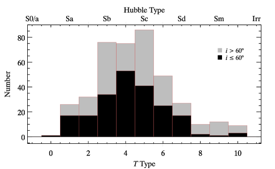
Figure 1: Distribution of morphological types for our selected sample and the parent sample of CGS spiral galaxies. The bottom axis gives the morphological type index $T$, with the corresponding Hubble types shown on the top axis. Spiral galaxies with inclination angle $i\leq 60\arcdeg$ and $i>60\arcdeg$ are shown in black and grey histograms, respectively.

3 Characteristics of spiral arms

3.1 Strength of Arm Structure

1D Fourier decomposition of the azimuthal light profile of isophotes can effectively reveal the non-axisymmetric structure present in galactic disks. This technique has been widely used in both observations and simulations (e.g., Elmegreen et al., 1989, 2007, 2011; Rix & Zaritsky, 1995; Grosbøl et al., 2004; Durbala et al., 2009; Kendall et al., 2015; Baba, 2015; Hu & Sijacki, 2016). The azimuthal light profile of isophotes naturally reflects the non-axisymmetric components of a galaxy. This method has the advantage that no prior assumption is made about the shape of the spiral arm. We study the harmonic components to analyze the strength, number, pitch angle, and arm length of spiral structure. The star-cleaned images are free from the contamination of foreground stars and background galaxies and thus are excellent for studying spiral structure. We run the IRAF task ellipse on the star-cleaned images with fixed $e$ and PA, employing linear steps to extract the azimuthal light profile of the isophotes. Fourier decomposition follows

$$I(r,\theta)=I_{0}(r)+\sum_{m=1}^{6}I_{m}(r)\cos m(\theta+\phi_{m}),$$ (1)

where $I(r,\theta)$ is the azimuthal profile at radius $r$ in direction $\theta$, $I_{0}(r)$ is the azimuthally averaged intensity, and $I_{m}(r)$ is the cosine amplitude and $\phi_{m}$ the phase angle of each Fourier component. We perform Fourier decomposition up to $m=6$, because higher order modes are nearly negligible. The IDL routine FFT was used to calculate the initial guesses of the amplitude and phase angle of the Fourier components of each profile, and then the CURVEFIT routine was used to do the Fourier fitting with the initial guesses for $I_{m}(r)$ and $\phi_{m}$.

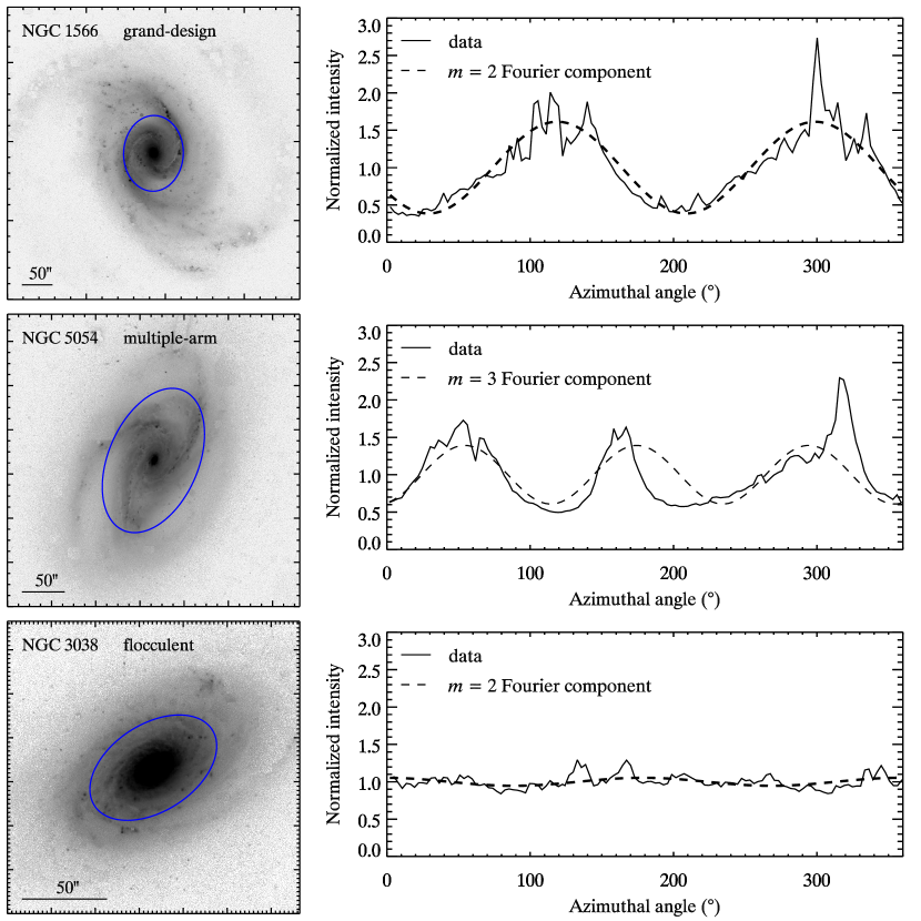
Figure 2: Illustration of the three main categories of spiral galaxies: (top row) grand-design galaxy NGC 1566, (middle row) multiple-armed galaxy NGC 5054, and (bottom row) flocculent galaxy NGC 3038. The images are oriented with north to the top and east to the left; a scale of 50^′′ is given in the bottom-left corner of each image. The left column shows the R-band CGS image. The blue ellipse denotes the isophote with which we extract the normalized azimuthal intensity profile in the right column. The dashed line represents the best-fit dominant Fourier mode.

Figure 2 (right panels) illustrates how the azimuthal light profile of an isophote, normalized by its mean intensity (solid line), can effectively characterize the relative amplitude of spiral arms. Three categories of spiral galaxies are illustrated: NGC 1566, a grand-design galaxy; NGC 5054, a multiple-armed galaxy; and NGC 3038, a flocculent galaxy. For each case, the Fourier mode with the highest amplitude is shown as a dashed line; the corresponding isophote on the 2D image on the left panels is marked by a blue ellipse. The Fourier mode properly reflects the amplitude of the non-axisymmetric structure in the disk, for different types of spiral arm structure, despite the presence of the sharp and localized features due to bright H II regions along the arms (see also Kendall et al., 2011).

The amplitude of the $m$th Fourier component relative to the axisymmetric component (the relative amplitude) is defined as

$$A_{m}(r)=\frac{I_{m}(r)}{I_{0}},$$ (2)

where $m=1,2,\cdots,6$. Figure 3 illustrates an example of the relative amplitudes of the first six Fourier modes as a function of radius for the grand-design spiral NGC 1566.

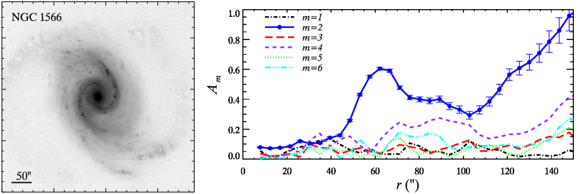
Figure 3: Illustration of the Fourier modes of the grand-design spiral NGC 1566. (Left) R-band CGS image, oriented with north to the top and east to the left; a scale of 50^′′ is given in the bottom-left corner. (Right) Relative amplitudes, $A_{m}$, of the first six Fourier modes ($m=1,2,\cdots,6$) as a function of radius. For the sake of clarity, we only show fitting errors for the $m=2$ mode.

The relative amplitude of the $m=1$ mode ($A_{1}$) reflects the lopsidedness of the galaxy (Rix & Zaritsky, 1995; Bournaud et al., 2005; Reichard et al., 2008), while the mean value of the $m=2$ mode ($A_{2}$) is usually used to represent the strength of arm structure for two-arm spiral galaxies (Grosbøl et al., 2004; Durbala et al., 2009; Elmegreen et al., 2011; Kendall et al., 2015). Some multiple-armed and flocculent galaxies, however, may have three or even four spiral arms. The $m=2$ mode alone is not enough to describe the arm strength for all the different types of spiral galaxies. Furthermore, the azimuthal light profile is not perfectly sinusoidal, which means that it will contribute not only to the dominant mode but also to other Fourier modes. Therefore, we use the quadratic sum of the $m=2,3$, and 4 relative amplitudes to represent the strength of spiral arms at radius $r$:

$$A_{\rm tot}(r)=\sqrt{A_{2}^{2}(r)+A_{3}^{2}(r)+A_{4}^{2}(r)}.$$ (3)

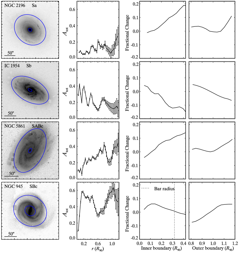
Figure 4: The effect of inner and outer boundary radius on the calculation of the strength of spiral arms. The left column shows the R-band CGS image, oriented with north to the top and east to the left; a scale of 50^′′ is given in the bottom-left corner. The outer blue ellipse marks $R_{90}$, and the inner blue ellipse marks the radius of the bar, if present, or $0.1R_{90}$ if not. The three columns to the right plot the arm strength $A_{\rm tot}$ as a function of radius and the fractional change of the arm strength as a function of the inner and outer boundary radius, normalized to $R_{90}$.

To calculate the mean value of $A_{\rm tot}$, we need to first specify the radial range over which the majority of the spiral arm structure is present. The spiral arms usually begin at the end of the bar or outside the bulge region and terminate at the outskirts of the galaxy. To facilitate the application of our method to future studies of galaxies drawn from large-scale imaging surveys, we require that the boundary of the arm structure should be robustly determined and not be very sensitive to observational conditions. Optical studies traditionally define the outer boundary of the galactic disk as the radius at which the B-band surface brightness is 25 mag arcsec^-2. However, $(1+z)^{-3}$ surface brightness dimming and uncertainties in the photometric zero point will induce systematic bias or uncertainty for this isophotal radius. A definition of radius that is independent of flux normalization, and thus independent of redshift and photometric calibration, is needed. The radius $R_{90}$, which contains 90% of the light from the galaxy curve of growth, naturally meets our requirements. Our simulated images in Section 4 (outer blue ellipse) demonstrate that $R_{90}$ is very robust, varying by less than 5% under a variety of observational conditions. Figure 4 (left column) illustrates that $R_{90}$ effectively encompasses the majority of the arm structure in galaxies of different types. On the other hand, the inner boundary of the arm structure in barred galaxies can be set naturally to the radius of the bar, if present. The bar radius is determined based on the large deviation of $e$ and PA near the bar region (Li et al., 2011). For unbarred galaxies, we use $0.1R_{90}$ to estimate the inner boundary of the arms. Visual inspection reveals that our choice of inner boundary (the inner blue ellipse in left column of Figure 4) closely delineates the beginning of the arms. Because the isophotes are extracted with fixed $e$ and PA, the presence of a bulge may induce a bimodal distribution in the azimuthal light profile, which may lead to an overestimation of the relative amplitude of the $m=2$ mode if the main bulge region is not excluded fully interior to $0.1R_{90}$. The third column of Figure 4 shows the fractional change of the arm strength when adopting different inner boundaries for different galaxy types (Sa to Sc), with the outer boundary fixed to $R_{90}$. There is no large systematic overestimation caused by the bulge, and the variation caused by the uncertainty in the determination of the inner boundary is $<10\%$. We also assess the impact of the adopted outer boundary. The fractional change of the arm strength (final column of Figure 4) is also $<10\%$ for different choices of outer boundary.

We calculate the mean strength of spiral arms over the radial range from either the bar radius or $0.1R_{90}$, depending on whether a not a bar exists, to $R_{90}$:

$$S=\frac{1}{N}\sum_{i=1}^{N}A_{\rm tot}(r_{i}),$$ (4)

where $N$ is the number of isophotes within the radial range. The associated uncertainty is set as the error of the average value. Similarly, we define the mean relative amplitude of the $m$th Fourier component:

$$S_{m}=\frac{1}{N}\sum_{i=1}^{N}A_{m}(r_{i}),$$ (5)

where $m=1,2,...,6$.

The mean strength of spiral arms may be color-dependent because young, blue stars are more concentrated in the arm regions than in the inter-arm regions. To better understand the wavelength dependence of mean arm strength, we compare in Figure 5 the relationship between mean arm strength in the I band ($S_{\it I}$) with that in B ($S_{\it B}$), V ($S_{\it V}$), and R ($S_{\it R}$) band. It is clear that the mean arm strength becomes systematically stronger from the I to the B band, qualitatively consistent with the notion that spiral arms trigger star formation (Roberts, 1969). The correlations between the arm strengths in different bands are very tight, with a small total scatter of 0.03. When using the arm strengths for any comparison studies, redshift or bandpass effects can be corrected according to the best-fitted linear relations given in the legend.

Figure 5: Upper row presents comparison between the mean strength of spiral arms measured in the I band ($S_{I}$) and that measured in the R ($S_{R}$, left), V ($S_{V}$, middle), and B ($S_{B}$, right) band. Bottom row presents the difference of the mean strength, $\Delta S=S_{R,V,\text{or}B}-S_{I}$, as a function of $S_{I}$. The solid line marks the best-fit linear relation, while the dashed line denotes $y=x$ and $\Delta S=0$ in the upper panels and bottom panels, respectively.

3.2 Pitch Angle and Length of Spiral Arm from 1D Method

Grand-design galaxies have two symmetric, long spiral arms. Some multiple-armed and flocculent galaxies can also have inner symmetric arms, but they split up into more fragmentary pieces at larger radii. Symmetric arm patterns may be wave modes obeying density wave theory. To quantitatively identify and study grand-design arms, we need to measure their pitch angle and length. Some studies (Grosbøl et al., 2004; Kendall et al., 2011) use 1D Fourier decomposition to calculate the pitch angle. The phase of a spiral wave can be identified by the phase angle of the $m=2,3,$ or $4$ Fourier mode, and the variation of the phase angle with radius can reveal useful information, such as the pitch angle of the spiral arm.

Our 1D method is based on the star-cleaned images and the phase angle from Equation (1). We begin by defining the region occupied by symmetric spiral arms as the “main” spiral region, within which the phase angle $\phi$ of the Fourier mode corresponding to the spiral pattern continuously increases or decreases with radius. The slope of the phase angle profile as a function of radius in this main spiral region reflects the tightness of the spiral arms. If a bar is present, the phase angle will remain almost constant before the main spiral region, then abruptly changes at the transition between the bar and arms; in the absence of a bar, the phase angle profile usually shows no regularity and can be identified easily. Beyond the main spiral region, the phase angle no longer changes monotonically. It can even become chaotic because the continuous arm structure terminates or transforms into feathery structures dominated by higher-frequency modes. We choose the Fourier mode that exhibits the most regular phase angle profile, showing the most nearly monotonic variation with radius, as the representative Fourier mode, $M_{\text{1D}}$, of the spiral pattern. We determine the main spiral region based on the behavior of the phase angle profile of Fourier mode $m=M_{\text{1D}}$. Since the cosine function in Equation (1) is symmetric, what we identify is the symmetric part of the spiral pattern. Assuming that the arms are logarithmic, the $\phi-r$ diagram of the main spiral region is fitted with a logarithmic function

$$\phi=b\cdot{\rm ln}\,r+{\rm const.},$$ (6)

where $\phi$ is the phase angle, $r$ is the radial distance from the center, and $b$ is a coefficient. The pitch angle $\varphi$ is given by

$$\varphi=\text{arctan}\left(\frac{1}{b}\right),$$ (7)

with its uncertainty determined through propagation of the fitting error of $b$. The length of the symmetric spiral pattern can be estimated from

$$L_{\rm arm}=\sqrt{1+b^{2}}\cdot\left(r_{\rm max}-r_{\rm min}\right),$$ (8)

where the $r_{\rm min}$ and $r_{\rm max}$ are the minimum and maximum radial extent of the main spiral region. The uncertainty of $L_{\rm arm}$ is determined through propagation of the fitting error of $b$.

Figure 6 shows an application of the method to measure the pitch angle and arm length for NGC 1566. The blue data points in the right panel denote the $m=2$ phase angle profile ($\phi_{\text{m}=2}$), and their corresponding positions on the spiral arms are shown in the left panel. The angle $\phi_{\text{m}=2}$ monotonically increases within the main spiral region $(30\arcsec,130\arcsec)$, over which the pitch angle and arm length can be calculated. The best-fit logarithmic function, marked by the solid red curve, gives a pitch angle of $19\fdg 5\pm 0\fdg 5$ and arm length of $298\arcsec\pm 7\arcsec$. A slight variation ($\sim 10\%$) of endpoints of the main spiral region will give rise to an uncertainty of $\sim 0\fdg 5$ and $\sim 6\arcsec$ for pitch angle and arm length, respectively, which are comparable with the uncertainties from the Fourier fitting.

A strong, underlying assumption of the above method is that the arm structure is dominated by a single ($m$th) Fourier mode. The method fails if the arm structure of the galaxy is very flocculent or if it is not symmetric at all, in which case there will be no main spiral region or continuously changing phase angle profile. Galaxies whose spiral arms are only marginally symmetric will have their symmetric part identified. Another shortcoming of this method is that it cannot identify the main spiral region if an arm runs almost parallel to the ellipse, as can occur in some strongly barred galaxies.

Table 1 lists $M_{\rm 1D}$, the radial range of the main spiral region, pitch angles, and arm lengths for 168 galaxies measured using the 1D method. We also give $S_{2,\text{main}}$, the mean relative amplitude of the $m=2$ mode in the main spiral region. We compute this quantity regardless of whether there are two arms or not. We expect $S_{2,\text{main}}$ to be stronger in grand-design galaxies than in non-grand-design galaxies. As demonstrated in Section 3.4, $S_{2,\text{main}}$ is very useful and effective to distinguish grand-design galaxies from other types, and thus can be used to probe the formation mechanism of spiral arms.

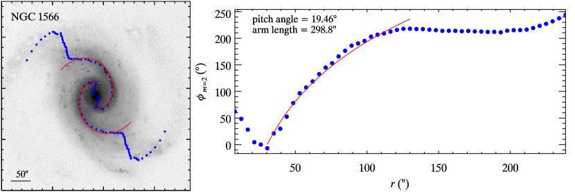
Figure 6: Illustration of our 1D method to measure the pitch angle of spiral arms. (Left) R-band CGS image of NGC 1566, oriented with north to the top and east to the left; a scale of 50^′′ is given in the bottom-left corner. The blue points mark the positions of the peak of the $m=2$ Fourier component, and the red line traces the best-fit logarithmic function. (Right) The $m=2$ phase angle profile (blue points) and the best-fit logarithmic function (red line). The derived pitch angle is 19$\fdg$46, and the arm length is 298$.\mkern-4.0mu^{\prime\prime}$8.

3.3 Pitch Angle from 2D Method

Another, more widely used technique to measure pitch angle is 2DDFT (Kalnajs, 1975; Iye et al., 1982; Krakow et al., 1982; Puerari & Dottori, 1992; Puerari, 1993; Block & Puerari, 1999; Seigar et al., 2005; Davis et al., 2012). The resulting pitch angle measurements from 1DDFT and 2DDFT are not necessarily the same, because the basic principle is different: the 1D method tries to identify the position of spiral arms and then fits a logarithmic function to those positions; the 2D method selects a 2D Fourier mode to represent the spiral arm. An important technical question arises: do these two methods give consistent results? In order to address this question and better understand the uncertainty induced by the different techniques, we also develop a 2D method based on 2DDFT to measure pitch angles.

We begin by deprojecting the galaxy image to face-on orientation. The sky background is first subtracted from the star-cleaned image. Then, with the PA and axis ratio ($1-e$) well defined, the galaxy is deprojected by rotating the sky-subtracted, star-cleaned image to align the major axis of the disk in the vertical direction and then using the IRAF routine geotran to stretch the x-axis by the axis ratio. This process assumes that the disk of the galaxy is intrinsically circular. To apply 2DDFT, the deprojected, sky-subtracted, star-cleaned galaxy image in Cartesian coordinates is transformed into an image in polar coordinates, and then the light distribution is decomposed into a superposition of sinusoidal functions of different frequency, with corresponding amplitude given by

$$A(m,p)=\frac{1}{D}\int^{\text{ln}(r_{\text{out}})}_{\text{ln}(r_{\text{in}})}\int^{\pi}_{-\pi}\sum_{j=1}^{N}I_{j}(r_{j},\theta_{j})\delta(\mu-\mu_{j})\delta(\theta-\theta_{j})e^{-i(m\theta+p\mu)}d\theta d\mu,$$ (9)

with $D$ a normalization factor expressed by

$$D=\sum_{j=1}^{N}I_{j},$$ (10)

where $I_{j}$ is the intensity of the $j$th pixel at $(r_{j},\theta_{j})$, $r_{\text{in}}$ and $r_{\text{out}}$ are the inner and outer radius of the spiral structure, respectively, $N$ is the number of pixels within the radial range, and $\mu\equiv{\rm ln}\,r$. For barred spiral galaxies, the spiral arms usually begin at the end of the bar. Although the bar lengths of CGS galaxies were provided by Li et al. (2011) using isophotal analysis, unfortunately these measured bar lengths do not always fully exclude the bar. Underestimation of bar length causes large overestimation of the pitch angle, if the bar length is adopted to represent the inner boundary of spiral arms. Davis et al. (2012) proposed to determine the inner radius by assuming the pitch angle is stable beyond the bar. However, the pitch angle can change with radius, by as much as 20% (Savchenko & Reshetnikov, 2013). To better determined the inner boundary of spiral arms, we first generate an unsharp-masked image by dividing the star-cleaned image by its blurred version, using, as kernel, a Gaussian function with full width at half maximum (FWHM) $0.1r_{\rm out}$, which is large enough to smooth large-scale structures such as a bar or spiral arms. This procedure effectively highlights the bar and spiral structure. Then we manually determine the inner radius after carefully avoiding the bi-symmetric component (bar or lens), which may induce a central peak in the resulting power spectrum and cause measurement errors. The outer radius is set to the radius where the spiral arms disappear, but 2DDFT is not sensitive to its adopted value.

Figure 7 presents the Fourier spectra (for radial range $[r_{\rm in},r_{\rm out}]$) for the deprojected images of NGC 1566 and IC 4538. In most cases, the resulting pitch angle is the pitch angle of the most prominent peak in the Fourier spectra. The grand-design galaxy NGC 1566 shows a dominant $m=2$ mode in its spectra, and thus $p$, corresponding to the highest amplitude ($|A(m,p)|$) indicated by the arrow, is used to calculate the pitch angle

$$\varphi=\arctan{\left(-\frac{m}{p}\right)}.$$ (11)

The upper-left panel of Figure 7 shows the deprojected image of NGC 1566 overplotted with a synthetic arm with a pitch angle of 21$\fdg$13 (its orientation is adjusted manually), illustrating that 2DDFT can accurately derive pitch angles for galaxies with clear and symmetric two-arm spirals. The resulting pitch angle is consistent with that obtained from 1DDFT (19$\fdg$46; Figure 6). However, for some multiple-armed or flocculent galaxies, the disk structure is so complicated that the highest amplitude does not contribute to the spiral pattern. The bottom-right panel of Figure 7 shows an example of Fourier spectra for this kind of galaxies. The highest amplitude of IC 4538 may correspond to some other bi-symmetric component, although it is inconspicuous in the deprojected image, or it may be just caused by the complicated spiral structure. If the most prominent peak were chosen to do the calculation, it would lead to a severely incorrect (usually overestimated) pitch angle. Instead, we identify the secondary maxima, the highest amplitude of the $m=4$ Fourier mode (purple arrow in Figure 7), to calculate a pitch angle of 19$\fdg$98, which produces synthetic arms that match well the deprojected image and is consistent with the value of 20$\fdg$0 derived from the 1D method. The 2D Fourier mode identified for further calculation is denoted as $M_{\rm 2D}$ in Table 1.

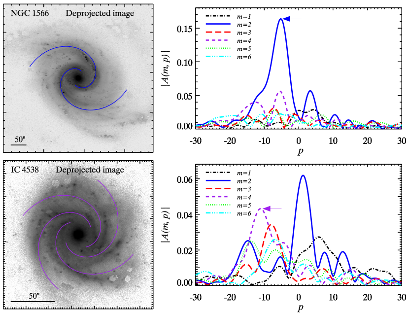
Figure 7: Illustration of our 2D method to measure the pitch angle of spiral arms. (Left) Deprojected R-band CGS images of NGC 1566 and IC 4538, oriented with north to the top and east to the left; a scale of 50^′′ is given in the bottom-left corner. (Right) Amplitude of the 2D spectra for the first six Fourier modes. The pitch angle is calculated from the peak of the $m=2$ mode in NGC 1566 and from the peak of the $m=4$ mode in IC 4538. The solid lines superposed on the deprojected images mark the synthetic arms with the resulting pitch angle.

If the arm structure is too irregular or too faint to be easily recognized, the Fourier spectra show large variation with no prominent peak, and the pitch angle is unmeasurable. The 2D method also fails if the arms deviate drastically from logarithmic shape, which may occur in galaxies with very long bars. We visually check the deprojected images of every galaxy overplotted with the synthetic arm pattern to verify the fidelity of the derived pitch angles.

2DDFT requires no prior knowledge of the light distribution. However, once we select the maxima amplitude of a particular Fourier mode $m$ to calculate the pitch angle, we do assume that the spiral structure can be represented by the symmetric, logarithmic $m$ Fourier component. Even though the spiral arms are not perfectly symmetric, as in the case of IC 4538 shown in Figure 7 (bottom-left panel), the 2D method can still correctly measure the pitch angle. If the arms deviate from a logarithmic function, the pitch angle changes with radius. We quantify the uncertainty introduced by this effect and that associated with the determination of the radial extent of the spiral arms by performing the 2DDFT with window functions. In addition to measuring pitch angle with radial bins $(r_{\text{in}},r_{\text{out}})$, we also repeat the calculation for another three radial bins: $(r_{\text{in}},r_{\text{out}}-0.2\Delta r)$, $(r_{\text{in}}+0.2\Delta r,r_{\text{out}})$, and $(r_{\text{in}}+0.1\Delta r,r_{\text{out}}-0.1\Delta r)$, where $\Delta r\equiv r_{\text{out}}-r_{\text{in}}$. Our final value of the 2D pitch angle is the average of these four estimates, with the uncertainty given by their standard deviation. The uncertainty due to the resolution of $p$ in Equation (9), which is set as 0.25 in this work, is negligible. Table 1 lists $M_{\rm 2D}$, radial range, and pitch angle measured using the 2D method for 159 galaxies.

We use both 1DDFT and 2DDFT to estimate the pitch angle of spiral arms. For galaxies with a continuous and symmetric arm pattern, like that of NGC 1566, both methods give consistent results. Galaxies with asymmetric or irregular arms, however, may produce different results for the two methods. Figure 8 gives a direct comparison between the pitch angles derived from both the 1D and 2D methods. A small, systematic trend may be present. For pitch angles $\lesssim 20\arcdeg$, the 1D method tends to yield somewhat larger pitch angles than the 2D method, whereas for pitch angles $\gtrsim 20\arcdeg$ the opposite seems to hold. However, the scatter between the two sets of measurements is only $\sim 2\arcdeg$, indicating that overall both techniques produce essentially consistent results.

The number of spiral arms could be set as the strongest 1D or 2D Fourier mode. Unfortunately, this cannot correctly describe the number of spiral arms. For example, IC 4538 clearly has four arms, but the strongest Fourier mode is $m=2$, both in 1D and 2D. The number of arms is taken to be the Fourier mode chosen to calculate the pitch angle: $M_{\text{1D}}$ and $M_{\text{2D}}$. They are not necessary the same, especially for some multiple-armed galaxies whose arms change from an inner two-arm structure into multiple arms in the outer region. The number of spiral arms is not well-defined in such cases. Therefore, we take $M_{\text{1D}}$ and $M_{\text{2D}}$ as the range of the number of spiral arms. The spirals of a few galaxies are strongly distorted by a long bar (e.g., NGC 1300); even though such galaxies have two arms, their pitch angle is unmeasurable and neither $M_{\text{1D}}$ nor $M_{\text{2D}}$ is available.

Figure 9 (upper row) plots the pitch angle against Hubble type. We confirm that the spiral arms on average tend to be more tightly wound in galaxies with earlier Hubble type, but with large scatter in pitch angle ($\sim 8\arcdeg$) for a given Hubble type. A dependence of pitch angle on Hubble type is expected in the context of density wave theory (Lin & Shu, 1964; Roberts et al., 1975; Bertin et al., 1989a, b). Our results are consistent with those of Kennicutt (1981), Ma (2002), and Kendall et al. (2015); no evidence of such correlation was found by Seigar & James (1998), which is partially due to their small range of measured pitch angle. There is no obvious correlation between pitch angle and Elmegreen arm class (bottom row of Figure 9).

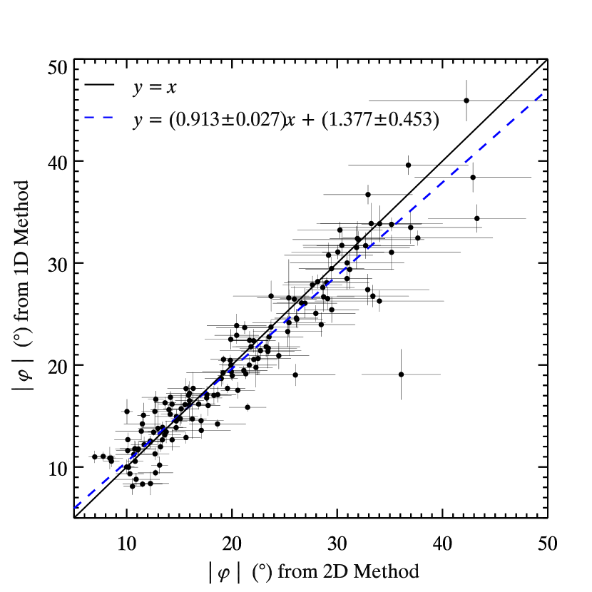
Figure 8: Comparison of pitch angles for 146 spiral galaxies, obtained from both the 1D and 2D methods. The black solid line denotes $y=x$, while the solid dashed line is the best-fit linear relation. The correlation has a scatter of $\sim 2\arcdeg$.

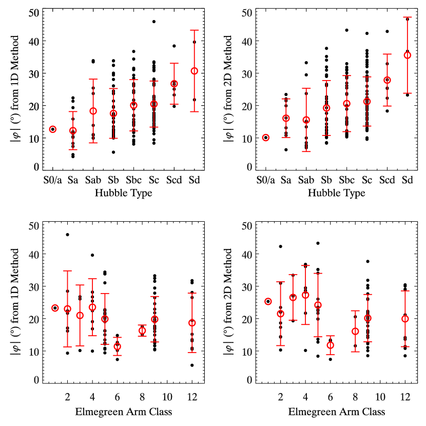
Figure 9: Dependence of pitch angle (left: 1D method; right: 2D method) on (top) Hubble type and (bottom) Elmegreen arm class. Spiral arm pitch angle decreases with earlier Hubble type, but with large scatter ($\sim 8\arcdeg$). Pitch angle does not correlate with Elmegreen arm class.

3.4 Comparison with Previous Studies

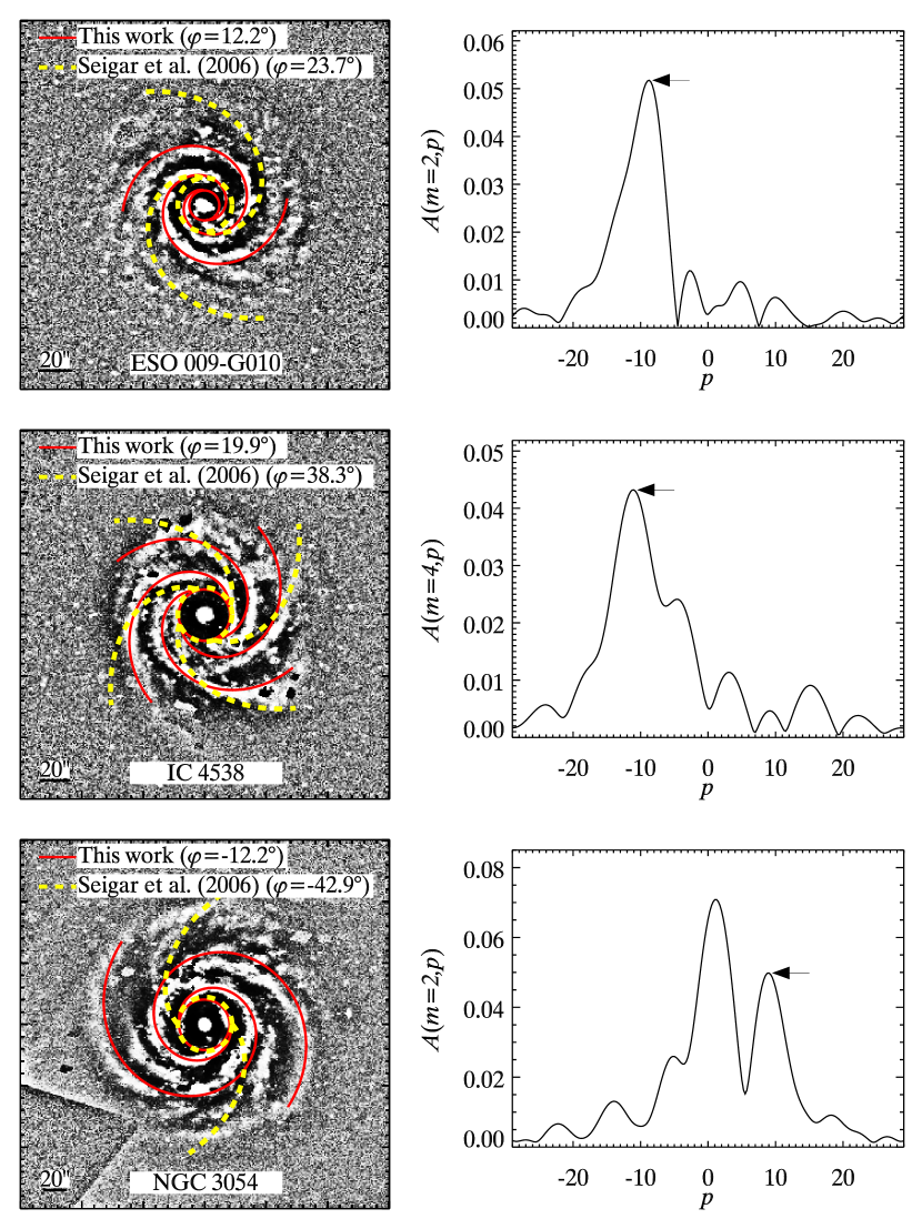
Figure 10: Illustration of our new pitch angle measurements for three galaxies in common with the study of Seigar et al. (2006). (Left) Unsharp-masked image overplotted with synthetic arms with our pitch angle (solid red curve) and that of Seigar et al. (2006; yellow dashed curve). The circles nearby the galactic center represent the innermost radial boundary. (Right) Fourier spectra for one of the four radial bins used to calculate the pitch angle, with an arrow indicating the peak chosen.

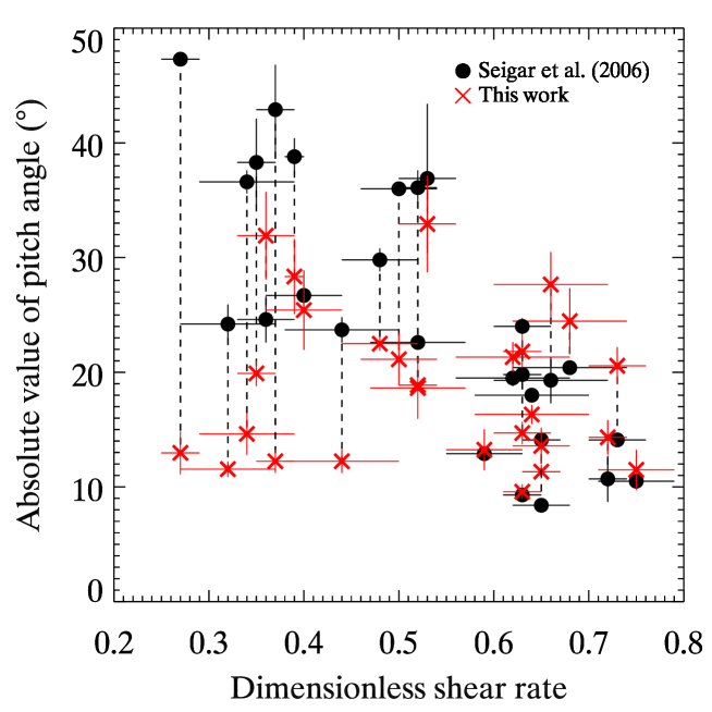
Figure 11: Correlation between shear rate and pitch angle. Black filled points are the results from Seigar et al. (2006), while red crosses represent our new measurements of pitch angle. Data points for the same galaxy are connected with a dashed line for comparison. Our new measurements show that the pitch angle correlates weakly, if at all, with the shear rate.

Seigar et al. (2005, 2006) report that the pitch angle of spiral arms strongly correlates with the shape of the galactic rotation curve, such that galaxies with open arms have rising rotation curves while those with tightly wound arms have falling rotation curves. The shape of the rotation curve is quantified by the dimensionless shear rate, defined by Seigar et al. (2005) as $\frac{1}{2}(1-\frac{R}{V}\frac{\text{d}V}{\text{d}R})$, where V and R are the local rotation velocity and radial distance from the galactic center, respectively. By contrast, the sample of 13 galaxies analyzed by Kendall et al. (2015) does not reveal a strong correlation between arm pitch angle and shear rate. As Seigar et al. (2006) make use of galaxy images from CGS, we can independently reexamine their results using our independent measurements of arm pitch angles.

Seigar et al. (2006) use 2DDFT to measure pitch angles for 31 CGS galaxies. Among these, 10 are not in our main sample because they do not satisfy our sample selection criteria. We uniformly analyze all the objects in the Seigar et al. (2006) sample, using, for consistency, the 2D method. We successfully measure pitch angles for 27 of the 31 galaxies. The spiral arm pitch angles derived by Seigar et al. (2006) are strongly overestimated (more than 10$\arcdeg$) for nine galaxies. For example, in the case of NGC 1566, Seigar et al. (2006) quote a pitch angle of $36.0\pm 0.3\arcdeg$, whereas we find $21.1\pm 2.2\arcdeg$, which is consistent with the value of $22\pm 2\arcdeg$ given by Kennicutt (1981) and $22.3\pm 0.1\arcdeg$ quoted by Kendall et al. (2011). For this galaxy, the overestimation of pitch angle by Seigar et al. (2006) is caused by improper projection parameters. The projection parameters we adopt ($e=0.21$, $\text{PA}=-2\arcdeg$) agree with those given by Kendall et al. (2011; $e=0.23$, $\text{PA}=3\arcdeg$), which were obtained by 2D bulge-to-disk decomposition using GALFIT. The discrepancy for the other eight cases, however, cannot be attributed to differences in adopted projection parameters, which are quite similar to ours. We verified that adopting the same projection parameters used by Seigar et al. (2006) does not resolve the discrepancy in pitch angles. As Figure 10 illustrates, the synthetic arms created using our pitch angles trace the spiral arms very well, and the galaxy images illustrate that the pitch angle from Seigar et al. (2006) are severely overestimated. Using our new pitch angle measurements of 27 galaxies and the shear rates given in Seigar et al. (2006), we redraw the scatter diagram for shear rate and pitch angle (Figure 11). The original data of Seigar et al. (2006; their Table 3) are shown for comparison. While our new measurements exhibit a weak trend between pitch angle and shear rate, they do not support the strong correlation reported by Seigar et al. (2006). Most of the large pitch angles ($>35\arcdeg$) reported by Seigar et al. (2006) were severely overestimated. Our results are quite similar to those of Kendall et al. (2015; their Figure 15).

Compared with previous studies, our pitch angles are more accurate, owing to careful determination of the radial range over which the measurements are made and, especially, the proper peak of the most relevant Fourier mode that represents the spiral arms. Our measurements lay the foundation for further quantitative studies on the dependence of spiral arms properties on galaxy properties.

3.5 Grand-design Spiral Arms

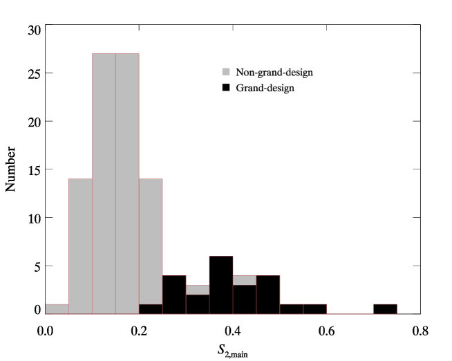
Figure 12: Distribution of mean relative amplitude of the $m=2$ mode in the main spiral region, $S_{2,\text{main}}$, for galaxies with a dominant $m=2$ mode. Results for grand-design galaxies are shown in the black histogram, while results for non-grand-design galaxies are shown in the grey histogram. $S_{2,\text{main}}$ is an effective, quantitative parameter to select grand-design galaxies.

Grand-design galaxies, as defined by Elmegreen & Elmegreen (1987, 1995), have two symmetric, long spiral arms dominating the galactic disk. However, some non-grand-design galaxies can also have two symmetric arms of sufficient prominence that can be considered grand-design, even if the spiral arms may not extend to the very outer parts of the disk. Grand-design spirals have a different formation mechanism than other arm classes. They may be arms dynamically triggered by the tidal force of a companion galaxy (e.g., Dobbs et al., 2010), or they may be wave modes obeying density wave theory (Lin & Shu, 1964; Bertin et al., 1989a, b). By contrast, irregular spiral structures may be the product of random gravitational instabilities generated by the gas and old stars in the disk (Goldreich & Lynden-Bell, 1965; Julian & Toomre, 1966; Kalnajs, 1971). Spiral structure that is marginally regular and relatively symmetric may be the result of a combination of different physical mechanisms. In our sample, only 109 of 211 galaxies have available arm class (AC) classifications in Elmegreen & Elmegreen (1987, 1995). We reclassify our galaxies with two clearly symmetric arms in I-band images as grand-design galaxies (Table 1). Most of our grand-design galaxies have AC 9 and 12, if available, with one galaxy designated AC 4. Some galaxies with AC 12 (e.g., NGC 1357) are classified as non-grand-design galaxies because their arms are not sufficiently dominant.

Here, we propose a new empirical, quantitative method to identify grand-design spirals. The main spiral region determined using the 1D method reflects the radial range where the grand-design spiral structure occupies. It should be strongly dominated by the $m=2$ Fourier mode. We define a new quantity, $S_{2,\text{main}}$, to denote the mean relative amplitude of the $m=2$ mode in this main spiral region for galaxies with a dominant $m=2$ mode. All those with dominant mode $m\neq 2$ are non-grand-design galaxies. Grand-design galaxies should have stronger $S_{2,\text{main}}$ than non-grand-design galaxies. Figure 12 shows the histogram of $S_{2,\text{main}}$ measured from R-band images. Two populations clearly emerge: those with $S_{2,\text{main}}\geq 0.25$ are grand-design galaxies; those with $S_{2,\text{main}}\lesssim 0.25$ are almost exclusively non-grand-design galaxies, although there are a few overlapping objects. Of the two non-grand-design galaxies that have $S_{2,\text{main}}>0.25$, one is strongly lopsided, leading to an exaggerated $m=2$ mode. One of the grand-design galaxies has relatively weaker spiral structure and thus a low value of $S_{2,\text{main}}$. Overall, $S_{2,\text{main}}$ appears to be an effective, quantitative parameter to select grand-design galaxies. We utilize this criterion to reclassify all the spiral galaxies in CGS. Table 1 lists the 23 cases that we consider to be grand-design spirals.

4 Simulated Images and Measurement Limit

The availability of large wide-field galaxy surveys allows us to use structural parameters of spiral arms to probe the formation and evolution of spiral structure in a much more statistical way. For instance, we can use resources available from SDSS to study the possible dependence of arm strength or pitch angle on other global galactic properties, including stellar mass, bulge-to-total light ratio, and environment. In the same spirit, we can extend the investigation to higher redshifts, using, for instance, images from CANDELS, to study the cosmic evolution of spiral structure. A practical limitation is that SDSS or CANDELS images may lose structural information because of resolution or signal-to-noise ratio (S/N) effects. Image degradation may be caused by instrumental or cosmological effects: exposure time, pixel size, point-spread function (PSF), cosmological dimming, or cosmological angular size. These effects can introduce possible measurement bias or uncertainty. In order to understand the limitations of our technique, we use high-quality CGS R-band images to simulate typical SDSS images and CANDELS images at various redshifts. We apply to these simulated images the same 1D and 2D Fourier analysis described in Section 3 to see how the image quality affects our measurements. Our analysis is similar in spirit to the work of Block et al. (2001), who investigated the effect of redshift on the 2D Fourier spectra of the spiral structure of NGC 922.

4.1 Simulated Images

To generate artificial SDSS and CANDELS images, we need to consider several observational parameters: redshift, PSF, sky noise, photometric zero point, exposure time, and pixel size. To simulate SDSS images, we use the parameters appropriate for an r-band observation, which has a pixel scale of $0\hbox{$.\mkern-4.0mu^{\prime\prime}$}396$, gain of 4.735, exposure time of 53.9 s, median Vega zero point of 23.94 mag, median PSF FWHM of $1\hbox{$.\mkern-4.0mu^{\prime\prime}$}4$, and a median sky background of $0.101904$ counts s^-1. These statistics were taken from the SDSS-DR7 photometric catalog (Abazajian et al., 2009). When generating the simulated images at higher redshift, the physical linear scale of the angular FWHM of the PSF and pixel size in CGS images cannot exceed that of the output simulated images. The minimum redshift of the simulated images is set as the redshift where both input PSF width and pixel size begin to match the output PSF and pixel size. The maximum redshift is set by the practical limitation of whether any useful structure can be resolved. As Figure 13 shows, spiral arms are nearly smoothed out in SDSS images by $z\approx 0.1$. We thus simulate SDSS images over the redshift range $0.01\lesssim z\lesssim 0.1$, in steps of $\Delta z=0.01$.

CANDELS targets five fields (GOODS-N, GOODS-S, UDS, EGS, and COSMOS) in two depths. The shallow portion of the survey (CANDELS/Wide) has exposures in all five fields; the deep portion (CANDELS/Deep) focuses only on GOODS-S and GOODS-N (Grogin et al., 2011). We therefore generate two sets of simulated images for CANDELS. The COSMOS images viewed with the Advanced Camera for Survey (ACS) Wide-Field Channel (WFC) detector in the F814W filter, with an exposure depth of 3.3 ks, are typical of CANDELS/Wide images. We use the COSMOS mosaic images (Koekemoer et al., 2011) to estimate the sky noise level of our simulated CANDELS/Wide images by averaging the sky noise in randomly selected sky regions. The GOODS-S deep field mosaic image viewed with ACS WFC has exposure depth up to 31.9 ks. To simulate the CANDELS/Deep images, we use the deepest portion of the GOODS-S deep field mosaic image (Koekemoer et al., 2011) to estimate the sky noise level. The final adopted parameters for simulating the CANDELS images are summarized in Table 2.

HST images have sufficiently high resolution that spiral structure in distant galaxies remains well-resolved. However, cosmological dimming is a factor, as is S/N. We simulate CANDELS images for a redshift range from $z=0.1$ to $z=1.1$, in steps of $\Delta z=0.1$. Starting with CGS images, we reduce their angular size, surface brightness, and resolution, adding random Poisson noise to mimic the properties of images observed at various redshifts by different instruments. At $z\approx 0.1$, the R band shifts into the V band, and at $z\approx 1.1$ the I band roughly maps into the B band. We do not consider k-correction. Empirical PSFs of CGS images are from Ho et al. (2011), while the PSF for the simulated SDSS images is approximated using a 2D Gaussian function with FWHM = $1\hbox{$.\mkern-4.0mu^{\prime\prime}$}4$ and for simulated CANDELS images a real PSF with FWHM = $0\hbox{$.\mkern-4.0mu^{\prime\prime}$}1$ is used.

The Poisson sky noise of CGS images is derived from the sky level calculated by Li et al. (2011). Our simulation procedure is summarized as follows:

Table 2: Parameters for the Simulated SDSS and CANDELS Images

Survey	Instrument	Band	Zeropoint	Exposure time	Sky noise	Pixel size	PSF FWHM	Gain
				(s)	(counts/s)	($\arcsec$)	($\arcsec$)
(1)	(2)	(3)	(4)	(5)	(6)	(7)	(8)	(9)
SDSS	—	r	23.94	53.9	0.101904	0.396	1.4	4.735
CANDELS/Wide	ACS/WFC	F814W	25.526	6900	0.00231366	0.03	0.1	1
CANDELS/Deep	ACS/WFC	F814W	25.526	32000	0.00107436	0.03	0.1	1

1. We rebin the CGS image and its associated PSF by taking into account the effect of pixel size and cosmological reduction of galaxy angular size. The rebinning factor is

   $$F_{\text{rb}}=\frac{n_{0}}{n^{\prime}}=\frac{d^{\prime}/(1+z^{\prime})^{2}}{d_{0}/(1+z_{0})^{2}}\cdot\frac{p^{\prime}}{p_{0}},$$ (12)

   where $n$, $d$, $z$, and $p$ represent the total pixel number, luminosity distance, redshift, and pixel size, respectively. The luminosity distance is calculated assuming $\Omega_{m}=0.3$ and $\Omega_{\lambda}=0.7$. The subscript 0 and prime superscript denote CGS parameters and corresponding simulation parameters, respectively.

2. We rescale the image flux with a rescale factor

   $$F_{\text{rescl}}=\left(\frac{d^{\prime}}{d_{0}}\right)^{2}\cdot 10^{0.4\cdot(z^{\prime}-z_{0})}.$$ (13)

   Here we consider the bolometric surface brightness dimming caused by the redshift effect and the cosmological evolution of surface brightness reported in Barden et al. (2005), who found that the surface brightnesses of galaxies at $z\approx 1$ are 1 magnitude brighter than those of galaxies in the local Universe.

3. We convolve the resulting images from step (2) with a Gaussian kernel to reach the desired output PSF. The kernel is calculated using Fourier deconvolution of the target PSF with the rebinned CGS PSF:

   $${\rm kernel}=\mathcal{F}^{-1}\left[\frac{\mathcal{F}\left({\rm PSF}_{\text{out}}\right)}{\mathcal{F}({\rm PSF}_{\text{in}})}\right],$$ (14)

   where $\mathcal{F}$ and $\mathcal{F}^{-1}$ represent Fourier transformation and inverse Fourier transformation, respectively. No convolution is applied if the two PSFs are comparable.

4. For simulating CANDELS images, the Poisson noise from the original CGS images is negligible after flux rescaling and PSF convolution, but it may become considerable in the case of simulating low-redshift SDSS images. Thus, the noise from the original CGS images is subtracted in quadrature from the target noise level, including sky noise and galactic flux noise, and then the resulting noise map is added to the images from step (3). We use the IRAF task mknoise to generated Poisson noise.

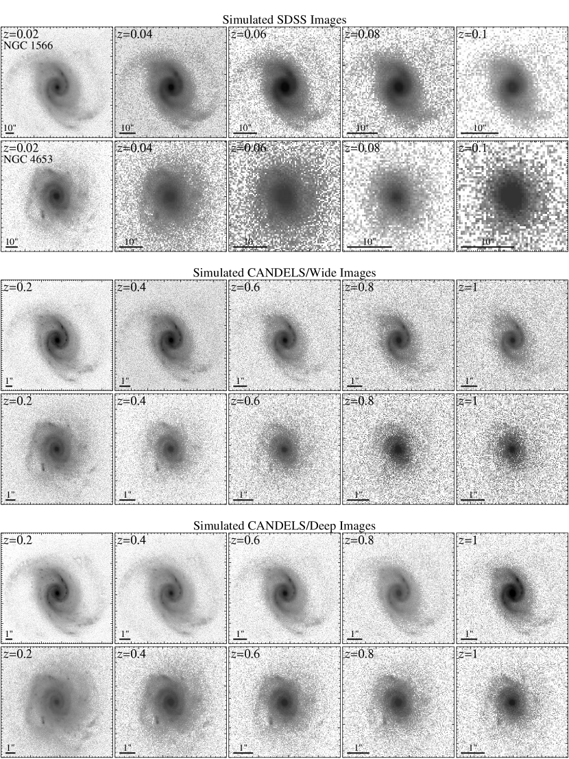
Figure 13: Nearby CGS galaxies NGC 1566 (grand-design) and NGC 4653 (non-grand-design) simulated to resemble observations by (top two rows) SDSS at $z$ = 0.02, 0.04, 0.06, and 0.1 and the HST CANDELS (middle two rows) Wide and (bottom two rows) Deep surveys at $z$ = 0.2, 0.4, 0.6, 0.8, and 1.

In Figure 13, the upper two rows present simulated SDSS images of the CGS galaxies NGC 1566 (grand-design spiral) and NGC 4653 (non-grand-design spiral), as viewed at $z=0.02$, 0.04, 0.06, and 0.1. The middle and bottom two rows pertain to simulated images under conditions similar to the CANDELS/Wide and CANDELS/Deep fields at $z=0.2$, 0.4, 0.6, 0.7, 0.8, and 1, respectively. For the simulated SDSS images, the two symmetric, strong arms of the grand-design galaxy can still be discerned at $z=0.1$, although they become quite blurred. The relatively weaker spiral structure of the non-grand-design galaxy is almost completely smoothed out by $z$ $\mathrel{\hbox{\hbox to0.0pt{\hbox{\lower 4.0pt\hbox{$\sim$}}\hss}\hbox{$>$}}}$ 0.06. By contrast, the resolution of the simulated HST images is good enough to recognize the inner part of the grand-design spiral structure in NGC 1566 out to at least $z\approx 1$, because this galaxy is intrinsically bright and the contrast between the arm and inter-arm region is high, while the structure information of non-grand-design spiral structure in NGC 4653 is nearly washed out by the noise at $z$ $\mathrel{\hbox{\hbox to0.0pt{\hbox{\lower 4.0pt\hbox{$\sim$}}\hss}\hbox{$>$}}}$ 0.6 in the CANDELS/Wide field. The CANDELS/Deep images obviously have better S/N and hence can go deeper.

4.2 Robustness of Measurements for the Simulated Images

The mean strength and pitch angle of spiral arms are the two most important parameters that can provide clues about the formation mechanism or evolution of spiral structure. Prior to any statistical study using SDSS or CANDELS images, an important step is to understand the robustness of the measurements under conditions that closely mimic those of the actual observations.

4.2.1 Robustness of Mean Arm Strength Measurement

Keeping $e$, PA, and bar radius as before for its CGS counterpart, we measure the mean strength of spiral arms following the same procedure described in Section 3 to extract the azimuthal light profile of isophotes. We then perform 1D Fourier decomposition to calculate the relative amplitudes of the Fourier modes, the phase angle profile of the $m=2$ Fourier mode, and $A_{\rm tot}(r)$. Figure 14 shows the results based on the grand-design galaxy NGC 1566, while Figure 15 displays the results for the non-grand-design galaxy NGC 4653, separately highlighting conditions appropriate for SDSS (left column), CANDELS/Wide (middle column), and CANDELS/Deep (right column). For the simulated SDSS images, the $A_{\rm tot}(r)$ profile gradually reduces in amplitude and becomes flattened with increasing redshift due to the smoothing effects of the PSF (Figure 13). The mean arm strength is therefore systematically underestimated. The behavior of the simulated HST images depends greatly on the intrinsic properties of the arms. In the case of grand-design spiral, its clear, distintive arms remain very well detected without any noticeable bias out to $z\approx 1$, both in the CANDELS Wide and Deep fields (Figure 14). The non-grand-design case fares far worse. Its lower contrast arms get lost in the noise for $z$ $\mathrel{\hbox{\hbox to0.0pt{\hbox{\lower 4.0pt\hbox{$\sim$}}\hss}\hbox{$>$}}}$ 0.6, beyond which $A_{\rm tot}(r)$ becomes divergent and the mean strength is severely overestimated (Figure 15).

To quantify the systematic bias in arm strength measurement, we calculate the difference between mean arm strength from the simulated SDSS/CANDELS images and that originally measured from the CGS images, for the full sample of 211 CGS galaxies. Figure 16 shows the difference of mean arm strength as a function of redshift. For every redshift bin, we obtain the mean value and the standard deviation as the measurement bias and uncertainty. The detailed values are listed in Table 3. The mean arm strength is reproducible within a reasonable scatter for the simulated SDSS and CANDELS images.

We note, in passing, that our method is of particular relevance for studies of the morphological trasformation of galaxies in galaxy clusters. Since the work of Butcher & Oemler (1978, 1984), it has been known that galaxy clusters as recent as $z\approx 0.4$ contain a much larger fraction of blue, mostly spiral galaxies than nearby clusters of similar richness and compactness, implying a strong morphological transformation from spirals to S0s (e.g., Dressler et al. 1994; Fasano et al. 2000). It would be of interest to apply our quantitative method in the context of these morphological studies, properly taking into account possible biases introduced by the observational effects investigated here.

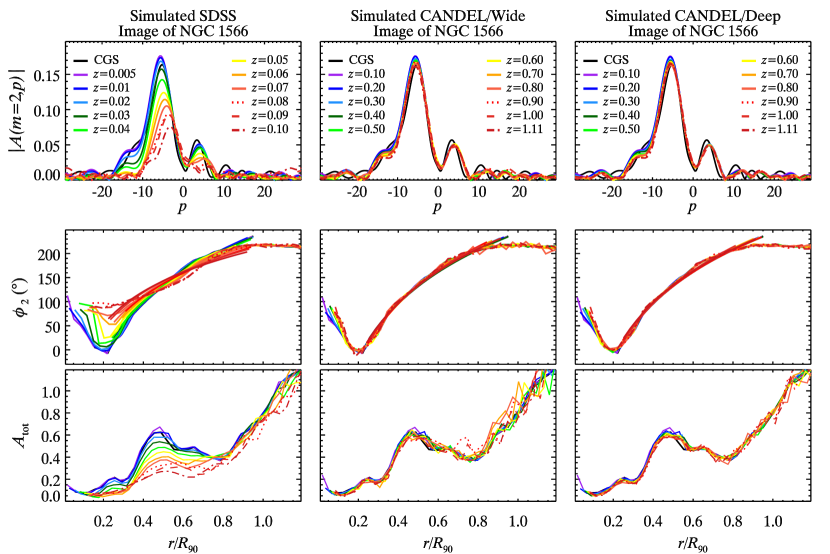
Figure 14: Spiral arm properties of NGC 1566 as measured from simulated images observed with (left) SDSS, (middle) CANDELS/Wide), and (right) CANDELS/Deep, for the redshifts indicated in the legends. The measured quantities are (top) the 2D Fourier spectra and radial profiles (normalized to $R_{90}$) of (middle) the phase angle of the $m=2$ Fourier mode and (bottom) the arm strength $A_{\rm tot}$.

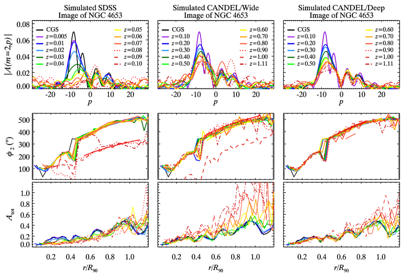
Figure 15: Spiral arm properties of NGC 4563 as measured from simulated images. Same convention as Figure 14.

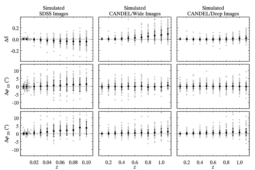
Figure 16: Difference between (top) the mean strength of spiral arms, (middle) 1D pitch angle, and (bottom) 2D pitch angle as measured in simulated images and observed images from CGS, as a function of redshift. The left, middle, and right columns simulate conditions appropriate for the SDSS, CANDELS/Wide, and CANDELS/Deep surveys, respectively. Solid points show the mean difference in each redshift bin, and the vertical bars represent the $1\sigma$ standard deviation.

4.2.2 Robustness of Pitch Angle Measurement

Lastly, we examine the robustness of pitch angle measurements to effects of resolution, noise, and redshift. We measure the pitch angle using both the 1D and the 2D techniques, following exactly the procedures outlined in Sections 3.2 and 3.3, respectively. For the 1D analysis, because of the degradation of image quality, the phase angle profile may not be the same as that of its CGS counterpart, and hence the main spiral region is redetermined according to the behavior of the phase angle profile. For the 2D analysis, we adopt the same deprojection, $e$, and PA as the CGS images, and we rescale the inner and outer boundary of the spiral structure of the CGS images by the rebinning factor.

The projection parameters of high-redshift galaxies can be readily determined using GALFIT, at least to $z\approx 2$. Davari et al. (2016) simulated two-component model galaxies to test the limits of measuring the structural components of massive galaxies, finding that the disk component can be measured with little difficulty even at $z=2$. Since 2D Fourier spectra are insensitive to the exact outer radius, the outer radius can be set simply as the radius where the spiral arms almost disappear. A more important source of uncertainty for high-redshift galaxies is the determination of the inner radius, especially in the presence of a bar. Fortunately, CANDELS images at $z$ $\mathrel{\hbox{\hbox to0.0pt{\hbox{\lower 4.0pt\hbox{$\sim$}}\hss}\hbox{$<$}}}$ 1 have sufficiently high resolution and depth that bars usually can still be discerned.

As image quality (especially spatial resolution) deteriorates, the spiral structure gets washed out by the PSF or noise. The 2D spectra have gradually less pronounced peaks and tend to become symmetric about $p=0$. The 1D phase angle profile increases in scatter. For sufficiently low resolution or S/N, the 1D phase angle profile and 2D Fourier spectra can become completely uninterpretable. These images were excluded. As expected, the number of galaxies for which pitch angle can be measured successfully decreases with increasing redshift (Table 3). For simulated SDSS images at $z=0.1$, pitch angles can be measured for only $\sim$ 20% of the original sample. Owing to the high resolution and depth of the HST observations, the success rate rises to $\sim$ 50% for CANDELS/Wide and $\sim$ 70% for CANDELS/Deep at $z=1.1$.

We give examples of the 1D phase angle profile of the $m=2$ Fourier mode and 2D Fourier spectra for the simulated images. In the case of the SDSS images of the grand-design galaxy NGC 1566 (Figure 14), its phase angle profile flattens as redshift increases, leading to systematic overestimation of the pitch angle. The same holds true for the Fourier spectra; the peak of the $m=2$ mode gradually shifts toward zero with increasing redshift, leading to larger and larger pitch angles. A similar effect was noted by Peng et al. (2017), who found preferentially larger pitch angles for simulated high-redshift galaxies. We see no systematic effects in the simulated CANDELS images. The SDSS image quality has far more adverse effects on the Fourier spectra than the phase angle profile of the non-grand-design galaxy NGC 4653 (Figure 15). Its Fourier spectra decay rapidly with redshift, becoming almost totally chaotic at $z$ $\mathrel{\hbox{\hbox to0.0pt{\hbox{\lower 4.0pt\hbox{$\sim$}}\hss}\hbox{$>$}}}$ 0.04, consistent with the visual appearance of the simulated images in Figure 13. Consequently, we exclude the simulated images for NGC 4653 with $z$ $\mathrel{\hbox{\hbox to0.0pt{\hbox{\lower 4.0pt\hbox{$\sim$}}\hss}\hbox{$>$}}}$ 0.04 from measuring pitch angle when using the 2D method. Even with HST-quality images, its phase angle profile gradually becomes chaotic in the outer parts, and slight shifts in the peak of the Fourier spectra lead to changes of pitch angle with redshift. Contribution from the $m=2$ mode is reduced gradually, and contamination from higher values of $p$ becomes more and more significant with increasing redshift. These trends are quantified explicitly in Figure 16 and in Table 3.

5 Summary

We use observations from CGS to develop a systematic method to quantify the main characteristics of galaxy spiral arms, including the arm number, mean arm strength, arm length, and pitch angle. The arm number and arm length reflect the dominant mode and continuity of the arms, whereas the mean arm strength reveals the relative contrast between spiral arms and axisymmetric disk components. Consistent with the expectation that young stars form preferentially in spiral arms, the mean arm strength is systematically stronger toward bluer bands. We devise an effective, new parameter, the relative amplitude of the $m=2$ Fourier mode in the main spiral region ($S_{2,\text{main}}$), to quantitatively identify galaxies with grand-design spiral arms. Grand-design spirals may owe their origin to external dynamical perturbation and hence may be a useful probe of the near-field galactic environment. The pitch angle, which describes the tightness of the spiral arms, may reflect the underlying velocity field or mass distribution of the galaxy. We demonstrate that consistent pitch angles can be derived using either Fourier decomposition of the 1D azimuthal light profile of isophotes or from Fourier transformation of the 2D light distribution.

Our methodology can be applied to measure the statistical properties of spiral arms in large samples of galaxies, both in the nearby Universe to investigate their correlation with other physical properties and at higher redshift to study their possible cosmological evolution. To this end, we use the local high-quality CGS galaxy images to generate a series of simulated images to mimic observing conditions typical of the SDSS ($z$ $\mathrel{\hbox{\hbox to0.0pt{\hbox{\lower 4.0pt\hbox{$\sim$}}\hss}\hbox{$<$}}}$ 0.1) and HST/CANDELS (0.1 $\mathrel{\hbox{\hbox to0.0pt{\hbox{\lower 4.0pt\hbox{$\sim$}}\hss}\hbox{$<$}}}$ $z$ $\mathrel{\hbox{\hbox to0.0pt{\hbox{\lower 4.0pt\hbox{$\sim$}}\hss}\hbox{$<$}}}$ 1.1). We apply our analysis methods to these simulated images to understand the limits of their applicability and possible sources of systematic bias and uncertainty. SDSS-quality images are mainly limited by their relatively poor angular resolution. The mean arm strength tends to be underestimated and the measurement uncertainty of pitch angle reaches $\sim 5\arcdeg$. HST images typical of CANDELS, on the other hand, are mainly restricted by their relativelty low S/N. Nevertheless, both mean arm strength and arm pitch angle can be determined up to $z\approx 1$ without much significant bias or uncertainty.

References

- Abazajian et al. (2009) Abazajian, K. N., Adelman-McCarthy, J. K., Agüeros, M. A., et al. 2009, ApJS, 182, 543-558
- Baba (2015) Baba, J. 2015, MNRAS, 454, 2954
- Barden et al. (2005) Barden, M., Rix, H.-W., Somerville, R. S., et al. 2005, ApJ, 635, 959
- Barden et al. (2008) Barden, M., Jahnke, K., & Häußler, B. 2008, ApJS, 175, 105-115
- Bertin & Lin (1996) Bertin, G., & Lin, C. C. 1996, Spiral structure in galaxies a density wave theory, Publisher: Cambridge, MA MIT Press, 1996 Physical description x, 271 p. ISBN0262023962, ISBN0262023962
- Bertin et al. (1989a) Bertin, G., Lin, C. C., Lowe, S. A., & Thurstans, R. P. 1989a, ApJ, 338, 78
- Bertin et al. (1989b) Bertin, G., Lin, C. C., Lowe, S. A., & Thurstans, R. P. 1989b, ApJ, 338, 104
- Block et al. (1994) Block, D. L., Bertin, G., Stockton, A., et al. 1994, A&A, 288, 365
- Block & Puerari (1999) Block, D. L., & Puerari, I. 1999, A&A, 342, 627
- Block et al. (2001) Block, D. L., Puerari, I., Takamiya, M., et al. 2001, A&A, 371, 393
- Bottema (2003) Bottema, R. 2003, MNRAS, 344, 358
- Bournaud et al. (2005) Bournaud, F., Combes, F., Jog, C. J., & Puerari, I. 2005, A&A, 438, 507
- Butcher & Oemler (1978) Butcher, H., & Oemler, A., Jr. 1978, ApJ, 219, 18
- Butcher & Oemler (1984) Butcher, H., & Oemler, A., Jr. 1984, ApJ, 285, 426
- Byrd & Howard (1992) Byrd, G. G., & Howard, S. 1992, AJ, 103, 1089
- Carlberg & Freedman (1985) Carlberg, R. G., & Freedman, W. L. 1985, ApJ, 298, 486
- Conselice et al. (2011) Conselice, C. J., Bluck, A. F. L., Ravindranath, S., et al. 2011, MNRAS, 417, 2770
- Conselice (2003) Conselice, C. J. 2003, ApJS, 147, 1
- Davari et al. (2016) Davari, R., Ho, L. C., & Peng, C. Y. 2016, ApJ, 824, 112
- Davis et al. (2012) Davis, B. L., Berrier, J. C., Shields, D. W., et al. 2012, ApJS, 199, 33
- Davis & Hayes (2014) Davis, D. R., & Hayes, W. B. 2014, ApJ, 790, 87
- Dobbs et al. (2010) Dobbs, C. L., Theis, C., Pringle, J. E., & Bate, M. R. 2010, MNRAS, 403, 625
- D’Onghia et al. (2013) D’Onghia, E., Vogelsberger, M., & Hernquist, L. 2013, ApJ, 766, 34
- Durbala et al. (2009) Durbala, A., Buta, R., Sulentic, J. W., & Verdes-Montenegro, L. 2009, MNRAS, 397, 1756
- Elmegreen et al. (2007) Elmegreen, B. G., Elmegreen, D. M., Knapen, J. H., et al. 2007, ApJ, 670, L97
- Elmegreen et al. (1989) Elmegreen, B. G., Seiden, P. E., & Elmegreen, D. M. 1989, ApJ, 343, 602
- Elmegreen & Elmegreen (1987) Elmegreen, D. M., & Elmegreen, B. G. 1987, ApJ, 314, 3
- Elmegreen & Elmegreen (1995) Elmegreen, D. M., & Elmegreen, B. G. 1995, ApJ, 445, 591
- Elmegreen et al. (1999) Elmegreen, D. M., Chromey, F. R., Bissell, B. A., & Corrado, K. 1999, AJ, 118, 2618
- Elmegreen et al. (2011) Elmegreen, D. M., Elmegreen, B. G., Yau, A., et al. 2011, ApJ, 737, 32
- Fujii et al. (2011) Fujii, M. S., Baba, J., Saitoh, T. R., et al. 2011, ApJ, 730, 109
- Ghosh & Jog (2015) Ghosh, S., & Jog, C. J. 2015, MNRAS, 451, 1350
- Gillett & Mountain (1998) Gillett, F., & Mountain, M. 1998, Science With The NGST, 133, 42
- Goldreich & Lynden-Bell (1965) Goldreich, P., & Lynden-Bell, D. 1965, MNRAS, 130, 125
- Grogin et al. (2011) Grogin, N. A., Kocevski, D. D., Faber, S. M., et al. 2011, ApJS, 197, 35
- Grosbøl et al. (2004) Grosbøl, P., Patsis, P. A., & Pompei, E. 2004, A&A, 423, 849
- Ho et al. (2011) Ho, L. C., Li, Z.-Y., Barth, A. J., Seigar, M. S., & Peng, C. Y. 2011, ApJS, 197, 21
- Hu & Sijacki (2016) Hu, S., & Sijacki, D. 2016, MNRAS, 461, 2789
- Iye et al. (1982) Iye, M., Okamura, S., Hamabe, M., & Watanabe, M. 1982, ApJ, 256, 103
- Julian & Toomre (1966) Julian, W. H., & Toomre, A. 1966, ApJ, 146, 810
- Kalnajs (1971) Kalnajs, A. J. 1971, ApJ, 166, 275
- Kalnajs (1975) Kalnajs, A. J. 1975, La Dynamique des galaxies spirales, 241, 103
- Kendall et al. (2015) Kendall, S., Clarke, C., & Kennicutt, R. C. 2015, MNRAS, 446, 4155
- Kendall et al. (2011) Kendall, S., Kennicutt, R. C., & Clarke, C. 2011, MNRAS, 414, 538
- Kennicutt (1981) Kennicutt, R. C., Jr. 1981, AJ, 86, 1847
- Koekemoer et al. (2011) Koekemoer, A. M., Faber, S. M., Ferguson, H. C., et al. 2011, ApJS, 197, 36
- Krakow et al. (1982) Krakow, W., Huntley, J. M., & Seiden, P. E. 1982, AJ, 87, 203
- Li et al. (2011) Li, Z.-Y., Ho, L. C., Barth, A. J., & Peng, C. Y. 2011, ApJS, 197, 22
- Lin & Shu (1964) Lin, C. C., & Shu, F. H. 1964, ApJ, 140, 646
- Lin & Shu (1966) Lin, C. C., & Shu, F. H. 1966, Proceedings of the National Academy of Science, 55, 229
- Ma (2002) Ma, J. 2002, A&A, 388, 389
- Michikoshi & Kokubo (2014) Michikoshi, S., & Kokubo, E. 2014, ApJ, 787, 174
- Oh et al. (2008) Oh, S. H., Kim, W.-T., Lee, H. M., & Kim, J. 2008, ApJ, 683, 94-113
- Peng et al. (2010) Peng, C. Y., Ho, L. C., Impey, C. D., & Rix, H.-W. 2010, AJ, 139, 2097
- Peng et al. (2017) Peng, T., English, J. E., Silva, P., et al. 2018, MNRAS, submitted (arXiv:1707.02021)
- Puerari (1993) Puerari, I. 1993, PASP, 105, 1290
- Puerari & Dottori (1992) Puerari, I., & Dottori, H. A. 1992, A&AS, 93, 469
- Puerari et al. (2014) Puerari, I., Elmegreen, B. G., & Block, D. L. 2014, AJ, 148, 133
- Reichard et al. (2008) Reichard, T. A., Heckman, T. M., Rudnick, G., Brinchmann, J., & Kauffmann, G. 2008, ApJ, 677, 186-200
- Rix & Zaritsky (1995) Rix, H.-W., & Zaritsky, D. 1995, ApJ, 447, 82
- Roberts (1969) Roberts, W. W. 1969, ApJ, 158, 123
- Roberts et al. (1975) Roberts, W. W., Jr., Roberts, M. S., & Shu, F. H. 1975, ApJ, 196, 381
- Salo et al. (2015) Salo, H., Laurikainen, E., Laine, J., et al. 2015, ApJS, 219, 4
- Savchenko & Reshetnikov (2013) Savchenko, S. S., & Reshetnikov, V. P. 2013, MNRAS, 436, 1074
- Seigar & James (1998) Seigar, M. S., & James, P. A. 1998, MNRAS, 299, 685
- Seigar et al. (2005) Seigar, M. S., Block, D. L., Puerari, I., Chorney, N. E., & James, P. A. 2005, MNRAS, 359, 1065
- Seigar et al. (2006) Seigar, M. S., Bullock, J. S., Barth, A. J., & Ho, L. C. 2006, ApJ, 645, 1012
- Seigar et al. (2008) Seigar, M. S., Kennefick, D., Kennefick, J., & Lacy, C. H. S. 2008, ApJ, 678, L93
- Sellwood & Carlberg (1984) Sellwood, J. A., & Carlberg, R. G. 1984, ApJ, 282, 61
- Sheth et al. (2010) Sheth, K., Regan, M., Hinz, J. L., et al. 2010, PASP, 122, 1397
- Struck et al. (2011) Struck, C., Dobbs, C. L., & Hwang, J.-S. 2011, MNRAS, 414, 2498
- Thornley (1996) Thornley, M. D. 1996, ApJ, 469, L45
- Thornley & Mundy (1997) Thornley, M. D., & Mundy, L. G. 1997, ApJ, 484, 202
- Toomre (1969) Toomre, A. 1969, ApJ, 158, 899
- Toomre (1981) Toomre, A. 1981, Structure and Evolution of Normal Galaxies, 111
- Toomre & Toomre (1972) Toomre, A., & Toomre, J. 1972, ApJ, 178, 623
- York et al. (2000) York, D. G., Adelman, J., Anderson, J. E., Jr., et al. 2000, AJ, 120, 1579