SPECTROSCOPIC DETERMINATION OF CAPELLA’S PHOTOSPHERIC ABUNDANCES:
POSSIBLE INFLUENCE OF STELLAR ACTIVITY

Abstract

Capella is a spectroscopic binary consisting of two G-type giants, where the primary (G8 iii) is a normal red-clump giant while the secondary (G0 iii) is a chromospherically-active fast rotator showing considerable overabundance of Li as Li-enhanced giants. Recently, Takeda & Tajitsu (2017) reported that abundance ratios of specific light elements (e.g., [C/Fe] or [O/Fe]) in Li-rich giants of high activity tend to be anomalously high, which they suspected to be nothing but superficial caused by unusual atmospheric structure due to high activity. Towards verifying this hypothesis, we determined the elemental abundances of the primary and the secondary of Capella based on the disentangled spectrum of each component, in order to see whether any apparent disagreement exists between the two, which should have been formed with the same chemical composition. We found that the primary is slightly supersolar (by $\sim+0.1$ dex) while the secondary is subsolar (by several tenths dex) for heavier elements such as Fe, resulting in a marked discrepancy between the primary and secondary, though such a trend is not seen for light elements (e.g., C or O). These observational facts suggest that anomalously large [X/Fe] ratios found in Li-rich giants were mainly due to an apparent decrease of Fe abundance, which we speculate is caused by the overionization effect due to chromospheric UV radiation. We thus conclude that conventional model atmosphere analysis would fail to correctly determine the abundances of fast-rotating giants of high activity, for which proper treatment of chromospheric effect is required for deriving true photospheric abundances.

1 INTRODUCTION

Capella (= $\alpha$ Aur = HD 34029 = HR 1708 = HIP 24608) is a spectroscopic binary system (orbital period: 104 d) consisting of G8 iii and G0 iii giants, where the more evolved former/primary has a slightly larger mass and luminosity (2.6 $M_{\odot}$ and 79 $L_{\odot}$) than that of the latter/secondary (2.5 $M_{\odot}$ and 73 $L_{\odot}$). The primary is a typical late-G giant presumably in the He-burning stage (red clump), which is Li-deficient and a slow rotator as other normal giants. In contrast, the secondary is a fast rotator (projected rotational velocity is $v_{\rm e}\sin i\sim 35$ km s^-1) with high stellar activity (characterized by conspicuous chromospheric emission lines in UV; see, e,g., Sanad 2013), and shows a remarkably strong Li line, which indicates that the initial Li content is almost retained without being diluted (the surface Li composition for the secondary is by $\sim 100$ times as high as the primary). That is, the secondary star belongs to the unusual group of Li-rich giants.

Recently, Takeda & Tajitsu (2017; hereinafter referred to as Paper I) conducted a spectroscopic study on 20 Li-rich giants, in order to clarify their observational characteristic in comparison with a large number of normal red giants. According to their study, a significant fraction of Li-rich giants rotate rapidly and show high chromospheric activity (though less active slow rotators similar to normal giants do exist). Curiously, they found that abundance ratios of specific light elements (e.g., [C/Fe] or [O/Fe] derived from high-excitation lines) in such Li-rich giants of high rotation/activity tend to be unusually high (typically by several tenths dex) and do not follow the mean trend exhibited by normal red giants (see Figure 14 in Paper I). Since the initial compositions of these stars should not be so anomalous (most of the sample stars were of normal thin-disk population) and such overabundances of these elements are unlikely to be produced by dredge-up of nuclear-processed material, they suspected as a possibility that this anomaly is nothing but a superficial phenomenon (i.e., not the real abundance peculiarity) caused by unusual atmospheric structure due to high chromospheric activity.

It occurred to us that the Capella system is an adequate testbench to verify this hypothesis, because the primary is a quite normal giant star while the secondary is a Li-rich giant of high rotation and high activity. That is, these two components should have been formed with the same initial composition, and the abundances of the normal primary are expected to be reliably determined. Then, if we could detect any apparent discrepancy between the abundances of the primary and the secondary, we may state that some problem exists in the abundances derived for the secondary star, for which the standard procedure of conventional model atmosphere analysis would not be sufficient any more.

Unfortunately, despite that many papers have been published so far regarding the orbital elements and fundamental stellar quantities of the Capella system (see, e.g., Torres et al. 2009, 2015, and the references therein), spectroscopic studies on the photospheric abundances are apparently insufficient. Admittedly, the surface Li abundances of both components have already been clarified by several useful articles (e.g., Pilachowski & Sowell 1992, Torres et al. 2015, and the references therein), by which the distinct difference between them has been firmly established. However, few reliable studies appear to be available regarding Capella’s abundances of various elements other than Li. Somewhat surprisingly, even the metallicity (e.g., Fe abundance) of the sharp-lined primary star has not yet been established, for which considerably diversified results (from metal-poor through metal-rich) have been reported (cf. Torres et al. 2009, 2015, and the references). Above all, it is only Torres et al. (2015) that has ever conducted separate determinations of elemental abundances for the primary and secondary components, as far as we know.

This scarcity may be closely connected with the practical difficulty involved with Capella (double-line spectroscopic binary with components of similar luminosity), in which the line strengths become apparently weaker because of dilution. Moreover, determining the abundances of the secondary star is a very tough matter, because lines are appreciably wide and shallow due to large $v_{\rm e}\sin i$. In our opinion, precise abundance determination is hardly possible by directly working on the complex double-line spectrum. Therefore, the most promising way would be to use the adequately disentangled spectrum of each component, as recently done by Torres et al. (2015).

Motivated by this situation, we decided to carry out a detailed model-atmosphere analysis for the primary and secondary components of Capella, closely following the procedure adopted in Paper I, in order to see whether any meaningful difference exists in the photospheric abundances between these two stars. For this aim, the genuine single-line spectra for both stars were recovered by using the spectrum-disentangle method based on a set of original double-line spectra obtained at various orbital phases. The purpose of this paper is to report the outcome of this investigation.

The remainder of this article is organized as follows: We first explain our observational data in Section 2 and then the derivation of the disentangled spectra in Section 3. Section 4 describes the spectroscopic determination of atmospheric parameters by using the equivalent widths of Fe i and Fe ii lines as done in Paper I. In Section 5 are described the abundance determinations for the primary and secondary components (along with the Sun) by using two different approaches: spectrum-fitting method (as used in Paper I) and the traditional method using the equivalent widths. Section 6 is the discussion section, where the resulting abundances as well as their trends are reviewed and the implications from these observational facts are discussed. We also argue especially about the recent similar abundance study of Capella by Torres et al. (2015), because they reported a conflicting consequence with ours. The conclusions are summarized in Section 7. In addition, a supplementary section is also prepared (Appendix A), where we check from various viewpoints whether our disentangled spectra have been correctly reproduced.

2 OBSERVATIONAL DATA

Most of the observational data of Capella used for this study were obtained by spectroscopic observations of 11 times over 4 months in the 2015–2016 season by using GAOES (Gunma Astronomical Observatory Echelle Spectrograph) installed at the Nasmyth Focus of the 1.5 m reflector of Gunma Astronomical Observatory, by which spectra with the resolving power of $R\sim 40000$ (corresponding to the slit width of 2^′′) covering the wavelength range of 5000–6800 Å were obtained (33 echelle orders, each covering $\sim$ 70–90 Å). In addition, since these GAOES spectra do not cover the long wavelength region, we also used the spectrum (5100–8800 Å; $R\sim 100000$) obtained on 2010 April 29 by using the 1.88 m telescope with HIDES (HIgh Dispersion Echelle Spectrograph) at Okayama Astrophysical Observatory, which was used only for the analysis of O i 7771–5 lines.

The data reduction of these data (bias subtraction, flat-fielding, aperture-determination, scattered-light subtraction, spectrum extraction, wavelength calibration, and continuum-normalization) was performed using the “echelle” package of IRAF. The S/N ratios of the resulting spectra turned out sufficiently high (on the order of several hundred) in all cases. The Julian dates as well as the corresponding orbital phases of these spectra are summarized in Table 1.

3 SPECTRUM DISENTANGLING

For the purpose of obtaining the pure spectrum of each star to be used for our analysis, we made use of the public-domain software CRES written by S. Ilijić. This program extracts the pure single-line spectrum of each component based on a set of observed double-line spectra at various orbital phases by the spectrum disentangling technique formulated in the wavelength domain, which is computationally more time-consuming but more flexible than the one formulated in the Fourier domain (see, e.g., Simon & Sturm 1994; Hadrava 1995; Ilijić 2004; Hensberge et al. 2008).

It is necessary to know the radial velocities (local topocentric radial velocity; $V^{\rm local}$) of both the primary and secondary components for each spectrum as the input data to CRES. While $V_{\rm p}^{\rm local}$ for the sharp-lined primary can easily be determined, it is difficult to precisely establish $V_{\rm s}^{\rm local}$ for the secondary by direct measurement in the complex double-line spectrum, because lines are broad and shallow. Therefore, we adopted the following procedure. We first converted $V_{\rm p}^{\rm local}$ to $V_{\rm p}^{\rm hel}$ (heliocentric radial velocity) by applying the heliocentric correction ($\delta V^{\rm hel}$), and plotted such derived $V_{\rm p}^{\rm hel}$ against the orbital phase ($\phi$). Here, $\phi$ for each spectrum was computed by using the ephemeris of HJD($\phi=0$) = 2450857.21 + 104.02173$E$ ($E$: integer), where the origin as well as the orbital period were taken from Table 2 (CfA observation) and Table 9 of Torres et al. (2009). According to their best orbital solutions (where the velocity amplitudes are nearly the same and the eccentricity is almost zero), the $\phi$-dependences of $V_{\rm p}^{\rm hel}$ and $V_{\rm s}^{\rm hel}$ are expressed as

$$V_{\rm p}^{\rm hel}=+25.96(\pm 0.04)\cos(\phi)+29.66(\pm 0.04)\;\;({\rm km}\;{\rm s}^{-1})$$ (1)

and

$$V_{\rm s}^{\rm hel}=-26.27(\pm 0.09)\cos(\phi)+29.66(\pm 0.04)\;\;({\rm km}\;{\rm s}^{-1}).$$ (2)

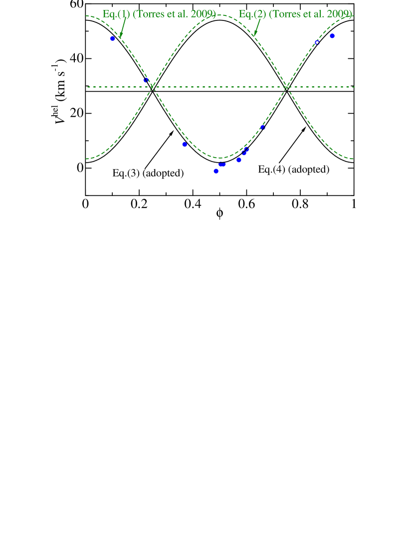
Figure 1: Symbols: heliocentric radial velocities of the primary ($V_{\rm p}^{\rm hel}$; cf. Table 1) corresponding to each of the 12 spectra (filled circles: GAOES data, open circle: OAO data), plotted against the orbital phase ($\phi$). Dashed lines: Torres et al.’s (2009) $V_{\rm p}^{\rm hel}(\phi)$ and $V_{\rm s}^{\rm hel}(\phi)$ relations [Equations (1) and (2)]. Solid lines: Finally adopted $V_{\rm p}^{\rm hel}(\phi)$ and $V_{\rm s}^{\rm hel}(\phi)$ relations [Equations (3) and (4)], in which the system velocity was slightly adjusted so as to fit better with the observed $V_{\rm p}^{\rm hel}$ (symbols).

However, we found that our $V_{\rm p}^{\rm hel}$ values did not necessarily match Equation (1) (cf. the dashed line in Figure 1). Therefore, we decided to slightly adjust the system velocity (by $-1.7$ km s^-1), and adopt the relation (with rounded coefficients)

$$V_{\rm p}^{\rm hel}=+26\cos(\phi)+28\;\;({\rm km}\;{\rm s}^{-1}),$$ (3)

for the primary, and its reflectionally symmetric curve for the secondary

$$V_{\rm s}^{\rm hel}=-26\cos(\phi)+28\;\;({\rm km}\;{\rm s}^{-1})$$ (4)

(cf. the solid lines in Figure 1). Further, making use of these symmetric relations, we simply put $V_{\rm s}^{\rm hel}$ as being equal to $56-V_{\rm p}^{\rm hel}$ (km s^-1) at each phase $\phi$, from which $V_{\rm s}^{\rm local}$ can be inversely evaluated by applying $\delta V^{\rm hel}$. We eventually confirmed that such evaluated $V_{\rm s}^{\rm local}$’s in combination with the measured $V_{\rm p}^{\rm local}$’s surely resulted in successful disentangling. (See also Section A.2 of Appendix A.) These radial velocities corresponding to each spectrum are summarized in Table 1.

In addition, we need to specify the flux ratio ($f_{\rm p}:f_{\rm s}$), which is wavelength dependent. Consulting Figure 1 of Torres et al. (2015), we assume $f_{\rm p}/f_{\rm s}$ = 0.84, 0.97, and 1.04 at 5000, 6000, and 7000 Å, respectively. The relevant $f_{\rm p}/f_{\rm s}$ to be passed to CRES was evaluated at the middle wavelength of the spectrum for each of the 33 echelle orders by applying quadratic interpolation.

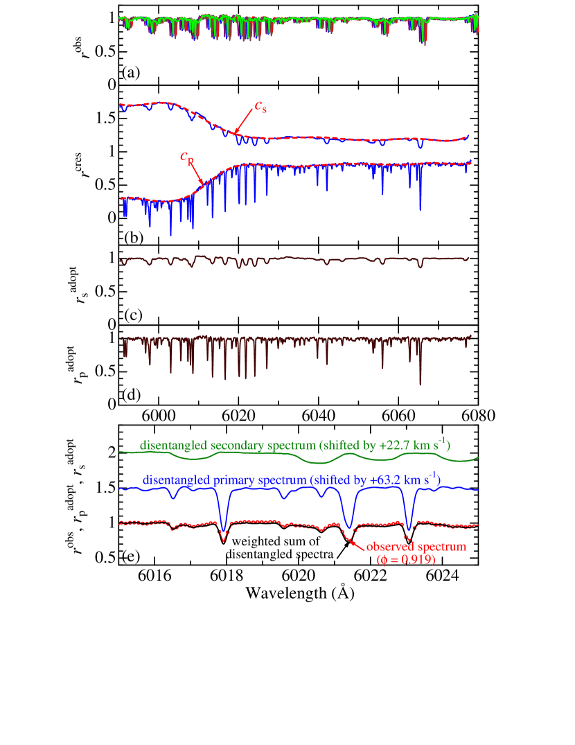
Figure 2: (a) Overplotted are the original 11 GAOES spectra ($r^{\rm obs}$; continuum-normalized residual flux in the 5900–6080 Å region) used for spectrum disentangling, where only the $\phi=0.504$ spectrum is highlighted in light green. (b) Solid lines: disentangled spectra of the primary ($r_{\rm p}^{\rm cres}$) and the secondary ($r_{\rm s}^{\rm cres}$), which were obtained as the direct output of CRES program. Dashed lines: apparent continuum ($c_{\rm p}$ and $c_{\rm s}$), which was defined as the envelope of $r_{\rm p}^{\rm cres}$ and $r_{\rm s}^{\rm cres}$, respectively. (c) Finally adopted disentangled spectrum of the secondary ($r_{\rm s}^{\rm adopt}$). (d) Finally adopted disentangled spectrum of the primary ($r_{\rm p}^{\rm adopt}$). (e) Demonstration of how the adopted disentangle spectra of the primary ($r_{\rm p}^{\rm adopt}$; top) and the secondary ($r_{\rm s}^{\rm adopt}$; middle) reproduce the original spectrum ($r^{\rm obs}$; open triangles; bottom) for the case of $\phi=0.919$, when combined by applying the appropriate shifts corresponding to the relevant $V_{\rm p}^{\rm local}$ and $V_{\rm s}^{\rm local}$ along with the adopted flux ratio (the resulting spectrum is depicted by the solid line at the bottom). Each spectrum in top, middle, and bottom is shifted by 0.5 relative to the adjacent one.

The basic dataset is the 11 continuum-normalized GAOES spectra ($r^{\rm obs}$) observed at various phases (Table 1), which are overplotted in Figure 2a (for the 5900–6080 Å region). Applying CRES to these spectra along with the relevant values of $V_{\rm p}^{\rm local}$, $V_{\rm s}^{\rm local}$, and $f_{\rm p}/f_{\rm s}$, we could obtain the disentangled spectrum for the primary ($r_{\rm p}^{\rm cres}$) and secondary ($r_{\rm s}^{\rm cres}$). As to the sampling, we adopted 0.025Å (almost equal to the original sampling) for the primary, while somewhat larger 0.05Å was adopted for the secondary. Note that the resulting $r_{\rm p}^{\rm cres}$ and $r_{\rm s}^{\rm cres}$ are not adequately normalized any more, as depicted in Figure 2b. This is because what is guaranteed by CRES is that the relation

$$r^{\rm obs}=f_{\rm p}r_{\rm p}^{\rm cres}({\rm shifted})+f_{\rm s}r_{\rm s}^{\rm cres}({\rm shifted})$$ (5)

($f_{\rm p}+f_{\rm s}=1$) holds, and thus ambiguities still exist in the absolute values of $r_{\rm p}^{\rm cres}$ and $r_{\rm s}^{\rm cres}$. Therefore, an appropriate offset correction has to be applied. For this purpose, we defined the apparent continuum (envelope) for $r_{\rm p}^{\rm cres}$ and $r_{\rm s}^{\rm cres}$, which we denote $c_{\rm p}$ and $c_{\rm s}$, respectively. Since this envelope level ($c$) should have been unity, we corrected $r^{\rm cres}$ to obtain the finally adopted disentangled spectrum ($r_{\rm p}^{\rm adopt}$ and $r_{\rm s}^{\rm adopt}$) simply as

$$r_{\rm p}^{\rm adopt}=(1-c_{\rm p})+r_{\rm p}^{\rm cres}$$ (6)

and

$$r_{\rm s}^{\rm adopt}=(1-c_{\rm s})+r_{\rm s}^{\rm cres},$$ (7)

as depicted in Figure 2c and Figure 2d, respectively.

We also checked whether the resulting $r_{\rm p}^{\rm adopt}$ and $r_{\rm s}^{\rm adopt}$ adequately reproduce the original spectrum ($r^{\rm obs}$) when added with the weights of $f_{\rm p}$ and $f_{\rm s}$ and shifted by $V_{\rm p}^{\rm local}$ and $V_{\rm s}^{\rm local}$. Such an example is demonstrated in Figure 2e (6015–6025 Å region; $\phi=0.919$), where we can see that a satisfactory match is accomplished. (See also Section A.1 of Appendix A.)

Although we confirmed that such obtained disentangled spectra are sufficiently clean and satisfactory in most of the wavelength regions, this procedure does not work well in specific spectral regions where strong telluric lines exist. Therefore, regarding the 6290–6310Å region comprising the important [O i] 6300 line, which is used for the spectrum-synthesis analysis, we specially removed the telluric line in the original $r^{\rm obs}$ by dividing by the spectrum of a rapid rotator before applying CRES, which turned out successfully. The complete set of finally adopted disentangled spectra ($r^{\rm adopt}$; 33 orders totally covering 4940–6790Å, plus special telluric-removed spectrum in the 6290–6310Å region) for the primary and secondary, which we used for this study, are presented as the online material (“spectra_p.txt” and “spectra_s.txt”).

4 ATMOSPHERIC PARAMETERS

Our determination of atmospheric parameters [effective temperature ($T_{\rm eff}$), surface gravity ($\log g$), microturbulence ($v_{\rm t}$), and metallicity ([Fe/H])] for the primary and the secondary was implemented by using the TGVIT program (Takeda et al. 2005b) in the same manner as described in Takeda et al. (2008; see Section 3.1 therein for the details) based on the equivalent widths ($W_{\lambda}$) of Fe i and Fe ii lines measured on the disentangled spectrum of each star. See Table E1 of Takeda et al. (2005b) for the list of Fe lines and their atomic data.

Regarding the sharp-lined primary star, the strengths of these Fe lines were measured by the Gaussian-fitting method, which was rather easy and worked quite well. However, measuring the equivalent widths of secondary star was a very difficult task, because almost all lines (considerably broadened due to large rotational velocity) more or less suffer contamination with other lines, and thus very few blend-free lines are available. Therefore, special attention had to be paid as described below:

• A specifically devised function was used for the fitting, which was constructed by convolving the rotational broadening function with the Gaussian function in an appropriately adjusted proportion.

• In order to decide whether a line is to be measured or not, we compared the stellar spectrum with the solar spectrum as well as with the theoretically computed strengths of the neighborhood lines by using the line list of Kurucz & Bell (1995).

• Judgement was done based on the following three criteria: (1) Does the wavelength at the flux minimum (i.e., line center) coincide with the line wavelength? (2) Is the line shape clearly defined as expected (whichever partial or total)? (3) Can we expect that the blending effect is not very serious (even though influence of contamination is more or less unavoidable)?

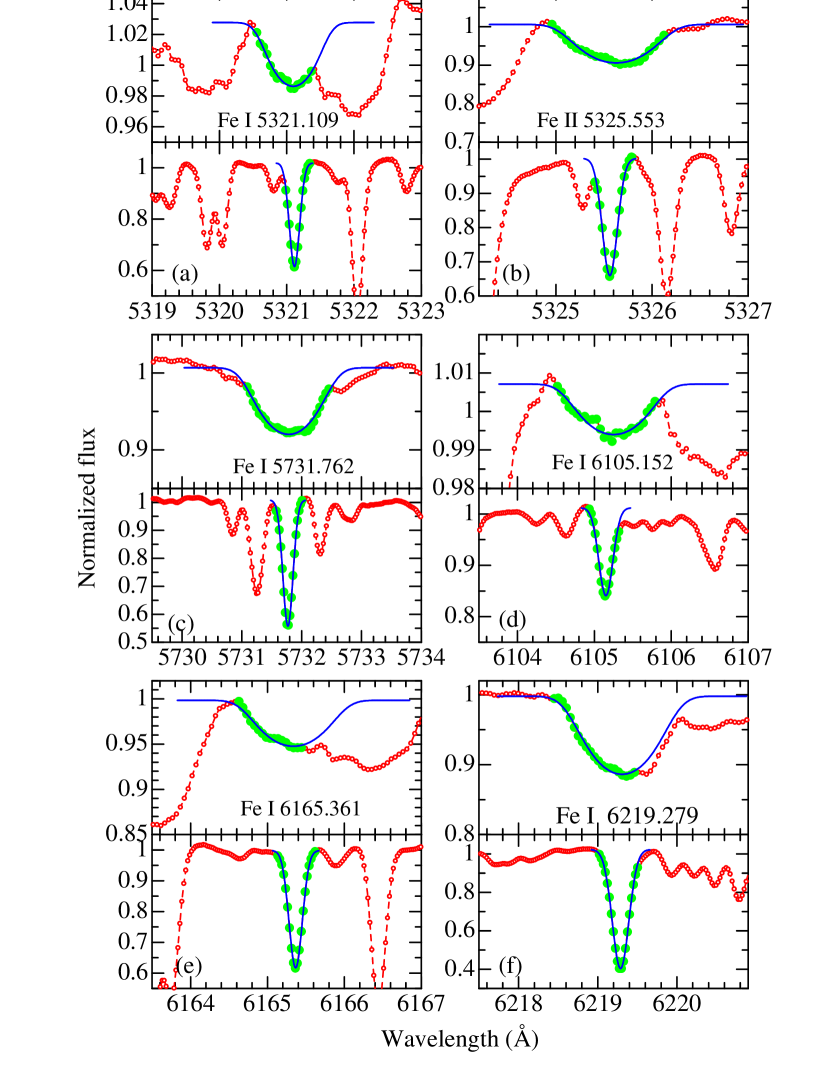
Figure 3: Examples of how we measured the equivalent widths for the secondary (upper panel) and the primary (lower panel). The observed data are shown by symbols, while the fitted function (rotational+Gaussian for the secondary and Gaussian for the primary) is depicted by solid lines. The part of the observed profile, which was used to determine the fitting function, are indicated by larger symbols in light green. (a) Fe i 5321.109, (b) Fe ii 5325.553, (c) Fe i 5731.762, (d) Fe i 6105.152, (e) Fe i 6165.361, and (f) Fe i 6219.279.

The actual examples of how we measured the equivalent widths are shown for the representative six lines in Figure 3, where we can see that rather tricky measurement had to be done in some cases of secondary stars (e.g., Figure 3e; which is the case judged to be barely measurable). In applying TGVIT, we restricted to using lines weaker than 120 mÅ and lines yielding abundances of large deviation from the mean ($>2.5\sigma$) were rejected in the iteration cycle, as done in Takeda et al. (2008).

The resulting parameters ($T_{\rm eff}$, $\log g$, $v_{\rm t}$) are $4943\pm 23$ K, $2.52\pm 0.08$ dex, $1.47\pm 0.13$ km s^-1 for the primary (from 147 Fe i and 16 Fe ii lines) and $5694\pm 73$ K, $2.88\pm 0.17$ dex, $2.29\pm 0.38$ km s^-1 for the secondary (from 52 Fe i and 6 Fe ii lines), where the quoted errors are internal statistical errors (see Section 5.2 in Takeda et al. 2002). The mean Fe abundance ($\langle A({\rm Fe})\rangle$) derived as a by-product (from Fe i lines) is $7.60\pm 0.05$ ([Fe/H] = $+0.10$) for the primary and $7.42\pm 0.08$ ([Fe/H] = $-0.08$) for the secondary, where the error is the mean error ($\equiv\sigma/\sqrt{N}$, where $\sigma$ is the standard deviation and $N$ is the number of lines). Note that, since the $gf$ values of the adopted lines are “solar $gf$ values” obtained by assuming $A_{\odot}$(Fe) = 7.50 (Takeda et al. 2005b), we can obtain the metallicity (Fe abundance relative to the Sun) as [Fe/H] = $A$(Fe) $-$ 7.50.

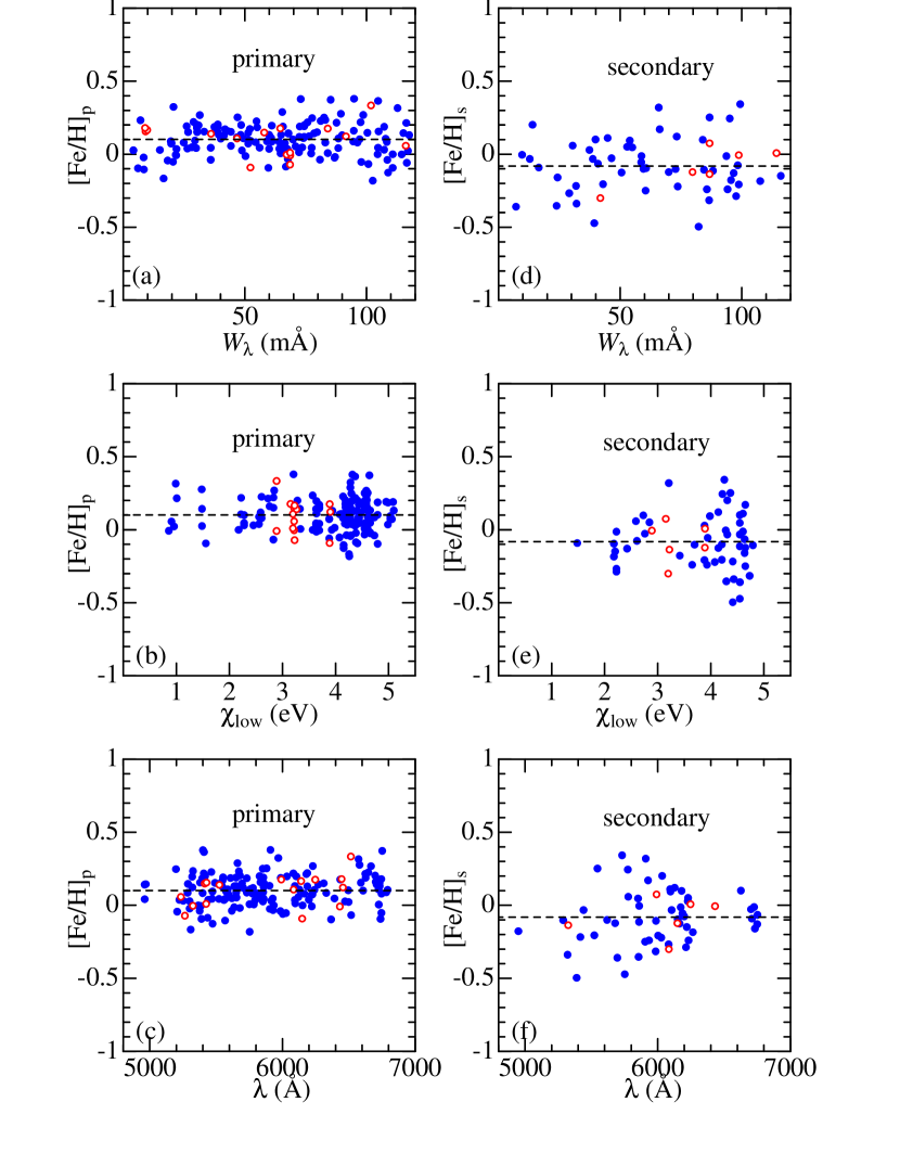
Figure 4: [Fe/H] vs. $W_{\lambda}$ (equivalent width) relation (upper panels: a, d), [Fe/H] vs. $\chi_{\rm low}$ (lower excitation potential) relation (middle panels: b, e), and [Fe/H] vs. $\lambda$ (wavelength) relation (bottom panels: c, f) corresponding to the finally established atmospheric parameters of $T_{\rm eff}$, $\log g$, and $v_{\rm t}$. The left-side panels (a, b, c) are for the primary while the right-side panels (d, e, f) are for the secondary. The filled and open symbols correspond to Fe i and Fe ii lines, respectively. The positions of the mean [Fe/H] (+0.10 for the primary and $-0.08$ for the secondary) are indicated by the horizontal dashed lines.

The $A$(Fe) values corresponding to the final solutions are plotted against $W_{\lambda}$ (equivalent width), $\chi_{\rm low}$ (lower excitation potential), and $\lambda$ (wavelength) in Figure 4, where we can see that no systematic trend is observed in terms of these quantities. We can thus confirm that the conditions required by the TGVIT program are reasonably fulfilled, which are the independence of $A$(Fe) upon $W_{\lambda}$ as well as $\chi_{\rm low}$ and the equality of the mean Fe abundances derived from Fe i and Fe ii lines. It is apparent from Figure 4 that the number of available lines is appreciably smaller ($\sim 1/3$) and the dispersion of the abundances is evidently larger for the secondary star (upper panels) compared to the case of primary (lower panels), which has caused the difference in the extent of parameter errors between two stars. This manifestly reflects the difficulty in measuring $W_{\lambda}$ of the secondary.

The detailed $W_{\lambda}$ and $A$(Fe) data for each line are given in “felines.dat” (supplementary online material). The model atmospheres for the primary and secondary stars to be used in this study were generated by interpolating Kurucz’s (1993) ATLAS9 model grid in terms of $T_{\rm eff}$, $\log g$, and [Fe/H]. Regarding the solar photospheric model used for determining the reference solar abundances (cf. Section 5), we also used Kurucz’s (1993) ATLAS9 model of the solar composition with $T_{\rm eff}$ = 5780 K, $\log g=4.44$, and $v_{\rm t}=1.0$ km s^-1.

5 ABUNDANCE DETERMINATION

5.1 Synthetic Spectrum Fitting

Closely following Paper I, we determined the abundances of various elements for the primary as well as secondary stars (and the Sun, for which the Moon spectra taken from the Okayama spectral database were used; cf. Takeda 2005a) by applying the spectrum-fitting technique and by carrying out a non-LTE analysis for several important elements (Li, C, O, Na, and Zn) based on the equivalent widths inversely determined from the best-fit abundance solutions. The selected wavelength regions are as follows: 5378.5–5382 Å (for C, Ti, Fe, Co), 6080–6089 Å (for Si, Ti, V, Fe, Co, Ni), 6101–6105 Å (for Li, Ca, Fe), 6157–6164 Å (for Na, Ca, Fe, Ni), 6297–6303 Å (for O, Si, Sc, Fe), 6361–6365 Å (for O, Cr, Fe, Ni, Zn), 6704–6711 Å (for Li, Fe), 6751–6760 Å (for S, Fe), and 7768–7786 Å (for O, Fe). See Paper I (Section 7 and Section 9 therein) for more detailed explanations of the procedures and the atomic data, which we adopted in this study almost unchanged. Regarding the macroscopic broadening function to be convolved with the intrinsic line profile, we adopted the rotational broadening function for the secondary star, while the Gaussian function was used for the primary star and the Sun. The different points compared to the case of Paper I are as follows:
— In the fitting involving the S i 6757 line, the wavelength range was made wider (6751–6760Å) to include the Fe i lines at $\sim$6752–6754Å, while $\sim$6754–6756Å region (where observed features can not be well reproduced by theoretical calculations) was masked.
— In the fitting involving O i 7771–5 triplet lines, we had to use the double-line spectrum (at $\phi=0.863$) observed by OAO/HIDES, because this triplet is outside of the wavelength range of the GAOES (i.e., disentangled) spectra. For this purpose, we modified our automatic solution-search program based on the algorithm described in Takeda (1995a), so that it may be applied to the combined spectra of primary and secondary components. Also, the wavelength range was chosen wider (7768–7786 Å) in order to cover the two spectra of considerable radial velocity difference.

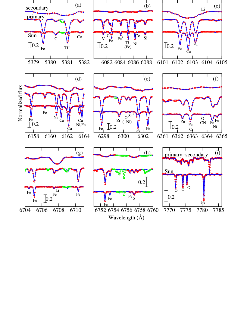
Figure 5: Synthetic spectrum fitting analysis carried out for 9 wavelength regions for abundance determinations. The observed spectra are plotted in red symbols (where the masked regions discarded in judging the goodness of fit are colored in light-green) while the best-fit theoretical spectra are shown in blue solid lines. (a) 5378.5–5382 Å region (for C, Ti, Fe, Co), (b) 6080–6089 Å region (for Si, Ti, V, Fe, Co, Ni), (c) 6101–6105 Å region (for Li, Ca, Fe), (d) 6157–6164 Å region (for Na, Ca, Fe, Ni), (e) 6297–6303 Å region (for O, Si, Sc, Fe), (f) 6361–6365 Å region (for O, Cr, Fe, Ni, Zn), (g) 6704–6711 Å region (for Li, Fe) (h) 6751–6760 Å region (for S, Fe), and (i) 7768–7786 Å region (for O, Fe). Note that telluric lines in the 6297–6303 $\rm\AA$ region (panel e) had been removed before the disentangling procedure was applied (cf. Section 3). Similarly, the broad Ca i autoionization feature in the 6361–6365 $\rm\AA$ region (panel f) was smoothed out by redrawing the continuum level.

How the fitted theoretical spectrum matches the observed spectrum (for the secondary, the primary, and the Sun) is displayed for each region in figure 5. The equivalent widths inversely derived from the abundance solutions and the non-LTE corrections for the important lines (C i 5380, Li i 6104, Na i 6161, Zn i 6362, S i 6757, and O i 7774) are given in Table 2. The finally obtained fitting-based abundances relative to the Sun for the primary ([X/H]_p) as well as the secondary ([X/H]_s), and the secondary$-$primary differential abundances [X_s/X_p] are presented in Table 3.

5.2 Abundances from Equivalent Widths

We also carried out differential analysis of the elemental abundances (other than Fe) of the primary as well as the secondary relative to the Sun, based on the equivalent widths of usable spectral lines, which were measured on the disentangled spectra as done in Section 4. The procedures of this analysis are detailed in Section 4.1 of Takeda et al. (2005c). Note that the solar equivalent widths used as the reference for this analysis were derived by Gaussian-fitting measurement on Kurucz et al.’s (1984) solar flux spectrum atlas. Regarding the primary, we measured the equivalent widths for 173 lines of 22 elements (C, O, Na, Al, Si, Ca, Sc, Ti, V, Cr, Mn, Co, Ni, Zn, Y, Zr, La, Ce, Pr, Nd, Gd, and Hf), while those of the secondary could be evaluated only for 27 lines of 9 elements (C, Al, Si, Ca, Sc, Ti, Cr, Ni, La), where the measurement was done in the same manner as the case of Fe lines described in Section 4. The resulting differential abundances relative to the Sun for each of the lines are separately summarized in “ewabunds_p.dat” (primary) and “ewabunds_s.dat” (secondary) of the online material.

We are afraid, however, that the number of available lines for each element is generally not sufficiently large and the appreciable fluctuation is often seen in the abundances, which makes the mean abundance less credible. Given that our purpose is (not to determine the abundances of as many element as possible but) to establish the abundance of any element as precisely as possible, we decided to confine our discussion to only those elements for which 7 or more lines are available (i.e., Si, Ca, Sc, Ti, V, Cr, Co, and Ni for the primary, and only Ni for the secondary). The resulting mean differential abundances of these elements and those of Fe (already derived in Section 4) are also summarized in Table 3.

6 DISCUSSION

6.1 Photospheric Abundances of Heavy Elements

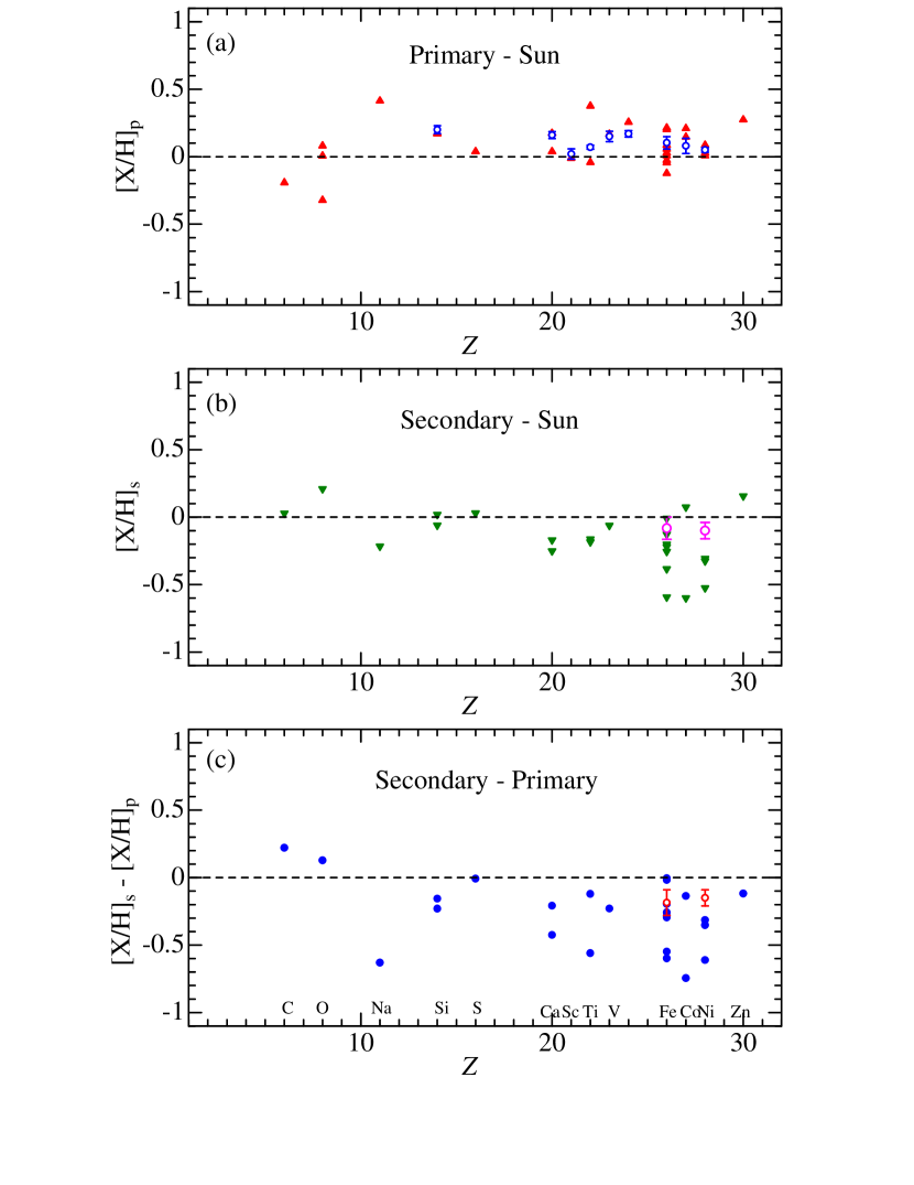
Figure 6: Differential abundances of various elements plotted against the atomic number ($Z$). The results derived from spectrum synthesis analysis are shown by filled symbols, while those from equivalent width analysis are by open symbols (attached error bar denotes the mean error $\sigma/\sqrt{N}$ as in Section 4). (a) Abundances of the primary relative to the Sun. (b) Abundances of the secondary relative to the Sun. (c) Abundances of the secondary relative to the primary. Note that the results for Li are not shown here.

The differential abundances relative to the Sun for the secondary ([X/H]_s), those for the primary ([X/H]_p), and the secondary$-$primary abundance differences ([X/H]${}_{\rm s}-$[X/H]_p), which were obtained in Section 5,1 and Section 5.2 and summarized in Table 3, are plotted against the atomic number ($Z$) in Figure 6. Hereinafter, we distinguish the “S”ynthesis-based abundance and equivalent-“W”idth based abundance by the superscript “S” and “W”, respectively, and the mean over available lines is denoted by the bracket “$\langle$” and “$\rangle$”.

We first discuss the heavier elements such as those of the Fe group ($Z\gtrsim 20$). Let us recall that we obtained $\langle$[Fe/H]${}_{\rm p}^{\rm W}\rangle=+0.10(\pm 0.05)$ and $\langle$[Fe/H]${}_{\rm s}^{\rm W}\rangle=-0.08(\pm 0.08)$ from determinations of atmospheric parameters based on Fe i and Fe ii lines (cf. Section 4): That is, the primary/secondary are slightly metal-rich/-poor by $\sim 0.1$ dex, which means that the metallicity of the secondary is less than the primary by $\sim 0.2$ dex.

This trend is confirmed also by abundances for other $Z\gtrsim 20$ elements shown in Figure 6. Regarding the primary, both of the $\langle$[X/H]${}_{\rm p}^{\rm S}\rangle$ and $\langle$[X/H]${}_{\rm p}^{\rm W}\rangle$ for each element is $\sim$ +0.1–0.2 dex, which almost agree with the case of Fe (cf. Figure 6a). As to the secondary, while the W-based abundance (only for Ni) is $\langle$[Ni/H]${}_{\rm s}^{\rm W}\rangle=-0.10$ and consistent with $\langle$[Fe/H]${}_{\rm s}^{\rm W}\rangle$, the S-based abundances for each element are somewhat more metal-poor to be $\langle$[X/H]${}_{\rm s}^{\rm S}\rangle\sim-$0.2–0.4 (see Figure 6b). In any event, we can conclude that, for heavier elements ($Z\gtrsim 20$), the primary is slightly metal-rich ($\langle$[X/H]${}_{\rm p}\rangle\sim+0.1$ to +0.2) while the secondary is apparently metal-poor ($\langle$[X/H]${}_{\rm s}\rangle\sim-0.1$ to $-0.4$; the extent being appreciably line-dependent), which means that the secondary is superficially metal-poor compared to the primary by several tenth dex (cf. Figure 6c).

Regarding the primary star, its marginally metal-rich nature (by $\sim$0.1–0.2 dex) is reasonably consistent with the fact that Capella belongs to the Hyades moving group (van Bueren 1952; Eggen 1960, 1972), because the metallicity ([Fe/H]) of this moving group is known to be slightly supersolar as +0.11 (Boesgaard & Budge 1988) or +0.07 (Fuhrmann 2011), in agreement with that of the Hyades cluster ($\sim$+0.1–0.2 dex; see, e.g., Takeda 2008; Takeda et al. 2013).

6.2 Behaviors of Light Elements

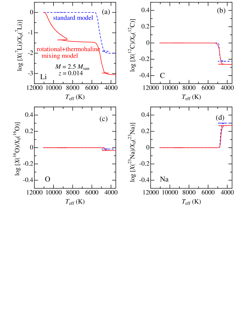
Figure 7: Run of the logarithmic surface abundances relative to the initial compositions ($\log[X/X_{0}]$) for selected light elements are plotted against $T_{\rm eff}$, which were theoretically simulated along the evolutionary sequence for the $M=2.5M_{\odot}$ solar-metallicity model by Lagarde et al. (2012), where two different treatments of envelope mixing were adopted: (i) standard mixing model (dashed line) and (ii) non-canonical model including rotational+thermohaline mixing with the initial rotation rate of $0.45\times$critical velocity (solid line). (a) ⁷Li, (b) ¹²C, (c) ¹⁶O, and (d) ²³Na.

Interestingly, such a tendency as shown by heavier species is not observed for lighter elements, as can be confirmed in Figure 6. Before discussing this trend, however, we should keep in mind that the surface abundance of light elements may have suffered changes due to a dredge-up of nuclear-processed material caused by evolution-induced mixing in the stellar envelope. This possibility is relevant for Li, C, O, and Na in the present case. For reference, we depict in Figure 7 how the surface abundances of these elements (main isotopes) are theoretically expected to undergo changes during the course of stellar evolution, which were simulated by Lagarde et al. (2012) for the standard mixing model and the special mixing model including rotational+thermohaline mixing.

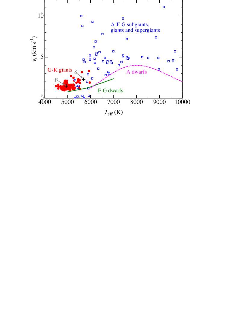
Figure 10: Microturbulence ($v_{\rm t}$) values of evolved stars plotted against $T_{\rm eff}$. Filled circles: G and early K giants (taken from Takeda et al. 2008; cf. Fig. 1d therein). Open squares: A–F–G subgiats, giants, and supergiants (taken from Takeda et al. 2018; abundance-based microturbulence denoted as $\xi_{\rm a}$; cf. Fig. 6b therein). Depicted in lines are the mean relations for dwarf stars (solid line $\cdots$ FG dwarfs, dashed line $\cdots$ A dwarfs; see Takeda et al. 2018 for more details). Our $v_{\rm t}$ values for the primary and the secondary are indicated by two crosses.

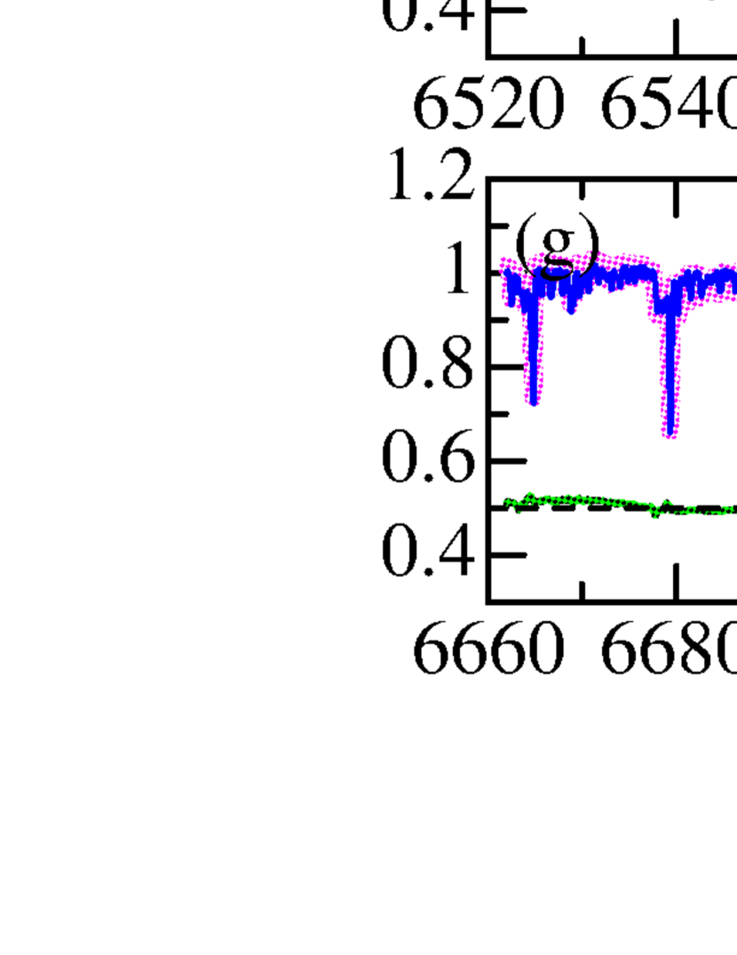
Figure 11: Comparison of the reconstructed primary+secondary spectrum ($r^{\rm rec}$; blue lines), which was simulated from the disentangled spectra ($r_{\rm p}^{\rm adopt}$ and $r_{\rm s}^{\rm adopt}$ being shifted with the relevant local radial velocities) by Equation (A1), with the actually observed double-line spectrum ($r^{\rm obs}$ at $\phi=0.919$; pink symbols). The green line shows the difference between these two spectra ($r^{\rm obs}-r^{\rm rec}$), where a vertical offset of 0.5 has been applied (the zero level is indicated by a dashed line and the origin is marked in the right-hand axis). The left-hand panels show the spectra of six echelle orders [(a) 5160–5230 Å, (b) 5540–5615 Å, (c) 6055–6135 Å, (d) 6245–6335 Å, (e) 6290–6310 Å(similar to panel (d) but telluric lines were removed in advance of disentangling), (f) 6520–6610 Å, and (g) 6660–6750 Å], while the magnified spectra in selected narrow wavelength regions are depicted in the corresponding right-hand panels (a^′)–(g^′).

Regarding Li, we obtained $A_{\rm p}\simeq 1.0$ (primary) and $A_{\rm s}\simeq 3.2$ (secondary), which are almost consistent with the previous studies (see, e.g., Pilachowski & Sowell 1992 or Torres et al. 2015, and the references therein). This means that the former is within the expected range shown by normal giants while the latter is the typical abundance of Li-rich giants (cf. Figure 11 in Paper I). Let us postulate (as most previous studies argued) that the secondary is still on the way of ascending the red-giant branch and preserves the original Li composition without being diluted. Then, the following characteristics can be read from Figure 7:
— The secondary star should have rotated rather rapidly (presumably $v_{\rm e}\sim 100$ km s^-1) when it was on the main sequence, as expected from the current $v_{\rm e}\sin i$. This is almost the same initial rotation rate assumed by Lagarde et al. (2012; see Section 2.3 therein) for their rotational+thermohaline mixing model, which indicates a significant dilution of Li already just after evolving off main-sequence stage (cf. solid line in Figure 7a). Then, if the secondary suffered no dilution, we may state that Lagarde et al.’s (2012) rotational+thermohaline mixing model is not realistic (which overestimates the extent of mixing) but the standard mixing may be more adequate.
— Li is the most fragile species (which is destroyed by reaction with proton at a comparatively low temperature of $T\sim 2.5\times 10^{6}$ K) among all elements, and its surface abundance is quite vulnerable to mixing in the envelope (cf. Figure 7a). So, if Li is preserved in the surface of the secondary star, any other elements must retain their original composition at the time of star formation. We may thus state that the primordial abundances of C, O, and Na are kept unchanged in the photosphere of secondary star.
— On the other hand, we can reasonably assume that the primary star is a normal red-clump giant in the core He-burning stage, such as expected for many red giants studied by Takeda et al. (2015). According to their observational results (see Fig. 10 therein), we may regard that C is moderately deficient by $\sim 0.2$ dex, O is only slightly deficient by $\lesssim 0.1$ dex, and Na is mildly overabundant by $\sim 0.2$ dex, which are quite consistent with the predictions of theoretical simulations (cf. Figure 7).

Keeping this in mind, we can draw the following consequences by comparing the abundances of these light elements for the primary and the secondary stars:
— (1) Regarding carbon, the results of [C/H]${}_{\rm p}\sim-0.2$ and [C/H]${}_{\rm s}\sim 0.0$ are just consistent with the expectation mentioned above. This means that the correct photospheric C abundances could be derived from the C i 5380 line for both components.
— (2) As to the case of oxygen, only O i 7771–5 triplet lines are usable for comparing the O-abundances of both components. The abundances derived from this triplet are [O/H]${}_{\rm p}=+0.08$ and [O/H]${}_{\rm s}=+0.21$ for the primary and the secondary, respectively; the latter being slightly larger (by $\sim 0.1$ dex) than the former. Considering that the surface O abundance for the primary may have suffered only a slight decrease ($\lesssim 0.1$ dex) due to envelope mixing while the secondary should retain the original composition, we can recognize a reasonable consistency between the oxygen abundances of the primary and the secondary; its original composition would have been slightly supersolar ([O/H] $\sim$ 0.1–0.2) such as the case of [Fe/H]_p (indicating [O/Fe] $\sim 0$).
— (3) The sodium abundances derived from the Na i 6161 line are of particular interest, which turned out [Na/H]${}_{\rm p}=+0.41$ and [Na/H]${}_{\rm s}=-0.22$ for the primary and the secondary, respectively. Considering that the primary has experienced an enrichment of surface Na by $\sim+0.2$ dex due to dredge-up of nuclear-processed product as mentioned above, we may state that its primordial Na abundance should have been slightly supersolar by $\sim+0.2$ dex, which is consistent with other heavier elements such as Fe. On the other hand, the mildly subsolar tendency for the secondary ([Na/H]${}_{\rm s}\sim-0.2$) is hard to be reasonably explained. We have no other way than to consider that the sodium abundance for the secondary was erroneously underestimated by several tenths dex, presumably because the conventional model atmosphere analysis is not properly applicable any more to the secondary star.

6.3 Origin of Superficial Abundance Anomaly

Based on the observational results described in Section 6.1 and Section 6.2, we can judge whether or not our adopted standard method of analysis using LTE model atmospheres can yield the correct abundances of both components, which are summarized as follows.

• Regarding the primary (normal red giant of slow rotation and low activity), the conventional method of abundance determination turned out to be successfully applicable without any problem, by which the expected abundances could be reasonably derived.

• As to the secondary (rotating giant star of high chromospheric activity), apparently low abundances (erroneously low by several tenths dex) were derived for heavier elements ($Z\gtrsim 20$; such as those of Fe group) as well as for Na, though the extent of this apparent underabundance appears to appreciably depend on the used lines. That is, in order to obtain the correct photospheric abundances of the secondary star for these elements, some non-canonical method (e.g., by properly taking into account the chromospheric effect) has to be applied.

• However, reasonably correct abundances could be obtained even for the secondary star regarding C (from C i 5380) and O (from O i 7771–5) by our conventional non-LTE analysis.

Turning back to the question raised in Paper I (i.e., regarding the anomalously large abundance ratios such as [C/Fe] or [O/Fe] observed in Li-rich giants of high rotation and high activity) which motivated this investigation, we have arrived at a satisfactory solution: It was not the increase of the numerator (C or O) but the decrease of denominator (Fe) that caused the apparently peculiar abundance ratio. That is, Fe abundances of active Li-rich giants would have been erroneously underestimated.

Then, which mechanism is involved with this superficial abundance anomaly? How could the active chromosphere affect the line formation? In Paper I, we once speculated that the chromospheric temperature rise in the upper atmosphere might have strengthen the temperature-sensitive high-excitation lines of C or O, since such an intensification is actually expected for O i 7771–5 (e.g., Takeda 1995b). However, this should not be the case, because correct abundances were obtained for these light elements as mentioned above. We have to find the reason why unusually low abundances were obtained for Fe group elements as well as for Na under the condition of high chromospheric activity. In our opinion, the most promising mechanism may be the overionization caused by excessive UV radiation radiated back from the chromosphere. As explained in Takeda (2008), it is lines of minor population species such as Fe i (while the parent ionization stage is the major population such as Fe ii) that can be significantly weakened by overionization. From this point of view, those elements showing appreciable underabundances in the secondary star (Na and heavier $Z\gtrsim 20$ elements) are mostly derived from lines of neutral species of minor population with comparatively low ionization potential (this effect is irrelevant for C i 5380 and O i 7771–5 lines, because neutral stage is the dominant population for C as well as O due to their high ionization potential).

However, even if this scenario is relevant, it is not easy to evaluate how much correction is required to recover the true abundance, because it appears to considerably differ from line to line. While only the slightly subsolar value ([Fe/H]${}_{\rm s}^{\rm W}\simeq-0.1$) was derived from equivalent widths of weak to mildly strong lines ($W_{\lambda}\leq 120$ mÅ; cf. Section 4), those derived from spectrum synthesis ([Fe/H]${}_{\rm s}^{\rm P}$) were more metal-poor (even down to $\sim-0.5$ or lower) and diversified, which may be attributed to the fact that various lines (including strong saturated lines which form high in the atmosphere) are involved in the spectrum synthesis analysis. Besides, if an overionization effect by chromospheric radiation is important, it is expected to have an appreciable impact on Li lines (Li i 6708 and Li i 6104), because neutral Li is a minor population species (i.e., mostly ionized) due to its low ionization potential. If so, the true Li abundance of the secondary might be significantly higher than the value we derived (3.2 from Li i 6708), which makes us wonder whether it is consistent with the assumption that the primordial Li is retained in the secondary (i.e., some further Li-enhancement mechanism might be responsible?). In any event, much more things still remain to be clarified regarding spectroscopic abundance determination for giant stars of high chromospheric activity.

6.4 Adequacy Check of Our Analysis

6.4.1 Conflict with Torres et al. (2015)

As mentioned in Section 1, only a small number of spectropic studies have been published for Capella so far, as briefly summarized in Table 4 (see also Footnote 9 in Torres et al. 2009). Especially, to our knowledge, it is only the recent investigation of Torres et al. (2015) who carried out abundance determinations for a number of elements separately for the primary and secondary components, as done in this study. Therefore, it is worth discussing their results in detail in comparison with our conclusion.

Torres et al. (2015) determined the abundances for 22 elements for both components (and oxygen only for the primary) from the equivalent widths measured for many spectral lines (in 4600–6750 Å) on the disentangled spectra (which were processed in a manner similar to ours based on the 15 spectra taken from the ELODIE archive; cf. Moultaka et al. 2004). We recognize, however, a distinct discrepancy between their work and this study. They concluded that the abundances of most elements (except for Li) are nearly solar (within $\sim\pm 0.1$ dex) for both components, which means that no meaningful compositional difference was observed between the primary and the secondary (cf. their Figure 3). Thus, their conclusion is in serious conflict with our consequence.

Unfortunately, since Torres et al. (2015) did not publish any detailed data (e.g., equivalent widths, $gf$ values, and abundances for individual lines they used), it is impossible for us to verify their results. We would here point out two concerns regarding their analysis:
— First, the number of lines they used for abundance determination of each element is almost the same for the primary and the secondary (see their Table 2). This is hard to understand, because the number of measurable lines should be considerably smaller for the broad-lined secondary than for the sharp-lined primary (in our case, the number of lines usable for the secondary was about $\sim 1/3$ of that for the primary).
— Second, their way of deriving [X/H] (abundance relative to the Sun) was simply to subtract the reference solar abundance (taken from Asplund et al. 2009) from the absolute mean abundance (obtained by averaging the abundances from individual lines); i.e., their analysis is not a differential one, and thus directly suffer errors involved in $gf$ values.

6.4.2 Spectra and equivalent widths

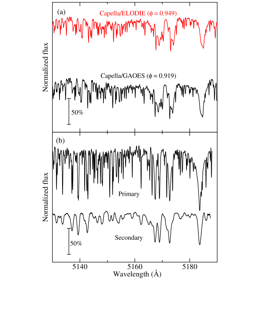
Figure 8: (a) Selected 5130–5190 Å portion of ELODIE spectrum of Capella (observed on 2003 March 25 corresponding to $\phi=0.949$; elodie_20030325_0023.fits) compared with that of our GAOES spectrum (observed on 2016 January 14 corresponding to $\phi=0.919$). (b) Our disentangled spectra for the primary and the secondary in the 5130–5190 Å region, which are to be compared with Torres et al.’s (2015) Figure 2.

In any event, given that such an conflicting result (near-solar abundances for both components) was once reported, we had better check whether something is different or wrong with our data and analysis, in comparison with that of Torres et al. (2015). Regarding the observational spectra of Capella, we can not see any significant difference between theirs and ours, not only for the original spectra (ELODIE vs. GAOES; cf. Figure 8a) but also for the disentangled spectra (Figure 8b, which appears almost consitent with Figure 2 of Torres et al. 2015).

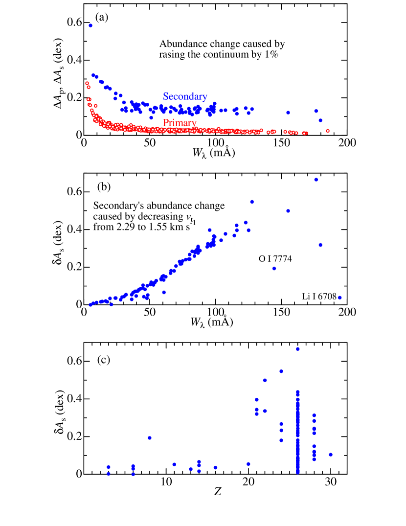
Figure 9: (a) Abundance variations ($\Delta A$) due to the changes in $W_{\lambda}$ caused by raising the continuum level by 1% (which were estimated as decribed in Section 6.4.2) plotted against $W_{\lambda}$. Open circles are for the primary and filled circles are for the secondary. (b) Abundance changes for the secondary ($\delta A_{\rm s}$) caused by using the microturbulence of $v_{\rm t}$ = 1.55 km s^-1 (the value used by Torres et al. 2015) instead of our adopted value of $v_{\rm t}$ = 2.29 km s^-1, plotted against $W_{\lambda}$. (c) Abundance changes for the secondary ($\delta A_{\rm s}$) in response to the reduction of $v_{\rm t}$ as in (b), plotted against the atomic number ($Z$).

There is a good reason to believe that our abundances for the sharp-lined primary are reliable because equivalent-width measurements are easy (see also Appendix A.3). However, considerable difficulties are involved for the broad-lined secondary as mentioned in Section 4. Is it possible that our $W_{\lambda}$ values (and thus the abundances) for the secondary might have been significantly underestimated; e.g., by incorrect placement of the continuum level? We checked this point by a simple test. If the continuum level is shifted by $\epsilon(\ll 1)$ as $f_{\rm c}\rightarrow f_{\rm c}(1+\epsilon)$, the line depth $R_{\lambda}(\equiv 1-f_{\lambda}/f_{\rm c})$ is changed as $R_{\lambda}\rightarrow R_{\lambda}[1+\epsilon(1-R_{\lambda})/R_{\lambda}]$. If we presume that the equivalent width of a line ($W_{\lambda}$) is proportional to its line-center depth ($R_{0}$), the expected change of $W_{\lambda}$ may be expressed as $W_{\lambda}\rightarrow W_{\lambda}[1+\epsilon(1-R_{0})/R_{0}]$. Assuming $\epsilon=0.01$ (i.e., raising the continuum by 1%), we examined how much abundance changes ($\Delta A$) would result for each line by this slight raise of the continuum, which are depicted in Figure 9a. We can see from this figure that only a slight change of the continuum level by 1% leads to a significant abundance variation by $\sim$ 0.2–0.3 dex for the secondary, while the abundance changes for the primary are insignificant (only a few hundredths dex for most cases) except for very weak lines. Therefore, we should keep in mind a possibility of appreciable systematic errors for the abundances of the secondary star if our continuum placement was not adequate, as far as abundances based on equivalent widths are concerned (i.e., those described in Section 4 and Section 5.2). Yet, we consider such a case rather unlikely, because the secondary’s abundances derived by using Takeda’s (1995a) spectrum-fittng method (Section 5.1), which is irrelevant to the continuum position, similarly turned out to be significantly subsolar.

6.4.3 Microturbulence

Regarding the atmospheric parameters, Torres et al.’s (2015) $T_{\rm eff}$ and $v_{\rm t}$ values were determined spectroscopically by using iron lines in a similar manner to ours, while they seem to have adopted the directly evaluated values for $\log g$. While we can see a reasonable consistency for $T_{\rm eff}$ and $\log g$ (cf. Table 4), an appreciable difference is observed for $v_{\rm t}$ of the secondary (though $v_{\rm t}$ for the primary is in agreement): that is, $1.55\pm 0.11$ km s^-1 (theirs) and $2.29\pm 0.38$ km s^-1 (ours). Actually, this difference of $\sim$ 0.7 km s^-1 is so large as to result in significant abundance changes, especially for strong saturated lines. In order to demonstrate this fact, we calculated the abundance differences for the secondary star ($\delta A_{\rm s}$) caused by using Torres et al.’s (2015) $v_{\rm t}=1.55$ km s^-1 instead of our 2.29 km s^-1, which are plotted against $W_{\lambda}$ (Figure 9b) and $Z$ (Figure 9c). We can see from Figure 9b that significant $W_{\lambda}$-dependent abundance variations (typically several tenths dex, even up to $\sim 0.6$ dex) are caused by this deacrease in $v_{\rm t}$. Moreover, according to Figure 9c, appreciably large increases of the abundances are typically seen for comparatively heavier elements ($Z>20$ species such as Fe group), while lighter elements ($Z\leq 20$) are not much affected because lines are not so strong. Combining Figure 6b with Figure 9c, we can see that the use of $v_{\rm t}=1.55$ km s^-1 would bring the secondary’s abundances nearer to the solar composition for most elements, except for the oxygen abundance derived from the O i 7774 line, which would become anomalously supersolar. Accordingly, it is likely that the difference in the adopted $v_{\rm t}$ is the main cause for the discrepancy in the secondary’s chemical composition between Torres et al. (2015) and this study.

Then, which of 2.29 km s^-1 and 1.55 km s^-1 is the correct $v_{\rm t}$ solution for the secondary? Considering the appreciably large abundance change ($\sim 0.4$ dex at $W_{\lambda}=100$ mÅ), the latter (low-scale) solution is definitely unlikely as far as our $W_{\lambda}$ data are concerned, because $W_{\lambda}$-independence of Fe abundances is successfully accomplished with the former (high-scale) solution (cf. Figure 4d).

From a different perspective, it is worthwhile to pay attention to the relative comparison of [$v_{\rm t}$(primary), $v_{\rm t}$(secondary)]: our analysis yielded markedly different values [1.47 km s^-1, 2.29 km s^-1], while Torres et al. (2015) derived almost the same results [1.48 km s^-1, 1.55 km s^-1]. Regarding evolved FGK giants, the behavior of microturbulence ($v_{\rm t}$) across the HR diagram (especially its $T_{\rm eff}$-dependence) was historically somewhat controversial. In the review paper of Gray (1978) was suggested a tendency of increasing $v_{\rm t}$ with $T_{\rm eff}$ for giants and supergiants (cf. Fig. 11 therein) based on the results of several studies published mainly in 1970s. Meanwhile, Gray (1982; cf. Fig. 11 therein) reported based on his line-profile analysis that $v_{\rm t}$ values of 4 late-type giants are almost $T_{\rm eff}$-independent at $\sim 1.5$ km s^-1. See also Fig. 3-8 in the lecture book of Gray (1988). However, considering that the behavior of“macro”-turbulence in FGK giants has been almost established to show an increasing tendency not only toward higher luminosity class but also toward earlier spectral types (see Fig. 17.10 of Gray 2005), we may expect similar trend to hold also for “micro”-turbulence. Actually, Takeda et al. (2008) showed that $v_{\rm t}$ values of GK giants (which were determined with the same procedure and line list as used in this study) tend to increase with $T_{\rm eff}$ at $T_{\rm eff}\gtrsim 5000$ K (cf. Fig. 1d therein). Besides, this trend naturally links to the distrbution of $v_{\rm t}$ for evolved A-, F-, and G-type stars recently determined by Takeda, Jeong, & Han (2018) from O i 7771–5 lines. This situation is illustrated in Figure 10, where our $v_{\rm t}$ results for the primary and secondary are also plotted by crosses. This figure reveals that these crosses reasonably follow the general trend, and thus $v_{\rm t}$ being larger for the secondary is quite natural. Consequently, our choice of high-scale $v_{\rm t}$ (2.29 km s^-1) for the secondary is considered to be justified, which may lend support to our conclusion.

7 CONCLUSION

Capella is a spectroscopic binary, which consists of two G-type giants with similar mass and luminosity. An interesting feature of this system is that, while the slightly more evolved primary (G8 iii) is a slowly-rotating normal red-clump giant, the secondary (G0 iii) is a chromospherically-active fast rotator ascending the giant branch and shows a marked overabundance of Li (i.e., Li-rich giant).

Recently, it was reported in Paper I that abundance ratios of specific light elements (e.g., [C/Fe] or [O/Fe]) in Li-rich giants of high activity tend to be anomalously high as compared to normal giants, which they suspected to be nothing but a superficial phenomenon (i.e., not real) caused by unusual atmospheric structure due to high chromospheric activity. The Capella system is a suitable testbench to verify this hypothesis; that is, if we could detect any apparent difference between the abundances of two stars, it may lend support for this interpretation, since we may postulate that both were originally born with the same chemical composition,

Toward this aim of searching for any apparent disagreement between the abundances of Capella’s two components, we carried out a spectroscopic analysis to determine the elemental abundances of the primary and the secondary of Capella. Since it is difficult to accomplish this task by working on the complex double-line spectra, we first recovered the genuine spectrum of the primary and that of the secondary by applying the spectrum-disentangle method to a set of original spectra obtained at various orbital phases.

The atmospheric parameters ($T_{\rm eff}$, $\log g$, and $v_{\rm t}$) of both stars were spectroscopically determined from the equivalent widths of Fe i and Fe ii lines as done in Paper I. Based on these parameters, we constructed the model atmospheres to be used for further abundance determination. The abundances of various elements were derived in two ways: (i) spectrum-fitting technique (as used in Paper I) applied to 9 wavelength regions, and (ii) analysis of equivalent widths as done by Takeda et al. (2005c).

We could clarify several significant observational facts and implications from the resulting abundances as itemized below, while postulating that (1) the primordial composition of the Capella system is the same for both components, (2) the primary star is a normal giant having suffered surface abundance changes due to envelope mixing in several specific light elements (Li, C, O, Na) and (3) the secondary star retains the original composition in its surface unchanged for all elements,

• We confirmed that the surface Li abundances are substantially different; $A_{\rm p}\sim 1.0$ (primary) and $A_{\rm s}\sim 3.2$ (secondary), as already reported by several previous studies, indicating that the former experienced a significant depletion while the latter retains the original Li composition.

• Regarding the heavier elements ($Z\gtrsim 20$) such as those of the Fe group, the abundances of the primary star turned out somewhat supersolar ([X/H]$\sim$ +0.1–0.2), which is consistent with the expectation because Capella belongs to the Hyades moving group. On the contrary, we found that the [X/H] values of the secondary are appreciably subsolar by several tenths dex (from $\sim-0.1$ down to $\sim-0.5$ or even lower) and diversified, which indicates an apparent disagreement exists between the abundances of the primary and the secondary.

• However, as to the light elements, such a tendency is not seen. For example, we can state that reasonably correct abundances of C (from C i 5380) or O (from O i 7771–5) could be obtained for both the primary and the secondary star by our conventional non-LTE analysis. Nevertheless, the exceptional case was Na (from Na i 6161), for which we found an unusual deficiency by several tenths dex for the secondary, despite that a reasonable abundance was obtained for the primary.

• Taking these observational facts into consideration, we think we could trace down the reason why anomalously large abundance ratios (such as [C/Fe] or [O/Fe]) were observed in Paper I for Li-rich giants of high rotation/activity. That is, it was not the increase of the numerator (C or O) but the decrease of denominator (Fe) that caused the apparently peculiar abundance ratios. In other words, Fe abundances of active Li-rich giants would have been erroneously underestimated.

• We note that lines yielding appreciable underabundances for the secondary star are mostly of minor-population species (e.g., neutral species such as Na i, Fe i, etc.) with comparatively low ionization potential. Accordingly, we suspect that the overionization caused by excessive UV radiation radiated back from the active chromosphere is responsible for the weakening of these lines, eventually resulting in an apparent underabundance.

• To conclude, the conventional model atmosphere analysis presumably fails to correctly determine the abundances of fast-rotating giants of high activity. A proper treatment of chromospheric effect would be required if true photospheric abundances are to be derived for such stars.

• To be fair, our consequence is in marked conflict with the similar abundance study on Capella recently carried out by Torres et al. (2015), who came to the conclusion that the photospheric abundances for the primary and the secondary are observed to be practically the same at the solar composition. Although we can not clarify the cause of this discrepancy because Torres et al. (2015) did not publish any details of their analysis, appreciably different values of adopted microturbulence for the secondary may be an important factor. Having examined this problem, however, we confirmed that our choice is reasonably justified, which may substantiate our conclusion.

Appendix A VALIDITY CHECK FOR THE DISENTANGLED SPECTRA

Since our abundance determination carried out in this paper is mostly based on the resolved spectra of the primary and secondary, which were disentangled with the help of the CRES program from a set of actually observed 11 spectra, it is important to ensure that this decomposition was correctly done. In this supplementary section, we present some additional information indicating that the spectra have been properly processed, where our attention is paid to (i) consistency between the reconstructed and original spectra, (ii) compatibility of the line widths ($v_{\rm e}\sin i$) for the secondary, and (iii) comparison of the equivalent widths of the primary with those of Hyades giants with similar parameters.

A.1 Matching test of reconstructed and original spectra

A simple and reasonable test to check whether this decomposition process has been adequately done is to compare the original double-line spectrum (at any phase) with the inversely reconstructed composite spectrum defined by the following relation (linear combination of the disentangled primary and secondary spectra).

$$r^{\rm rec}=f_{\rm p}r_{\rm p}^{\rm adopt}(v=v_{\rm p}^{\rm local})+f_{\rm s}r_{\rm s}^{\rm adopt}(v=v_{\rm s}^{\rm local}).$$ (A1)

Although this check was briefly mentioned in Section 3 for a restricted narrow wavelength range of 6015–6025 Å (cf. Figure 2e), we here show this comparison for further six echelle orders from shorter to longer wavelength ranges in Figures 11a,a^′–11f,f^′, where the runs of $r^{\rm rec}$, $r^{\rm obs}$, and their difference ($r^{\rm obs}-r^{\rm rec}$) with wavelength are depicted. We can see from these figures that the agreement between $r^{\rm rec}$ and $r^{\rm obs}$ is satisfactory in most cases, especially for longer wavelength regions (differences are $\lesssim 1\%$).

While we notice an appreciably undulated difference (up to $\lesssim 10\%$) in shorter wavelength regions (cf. Figures 11a and 11b), this is not due to the disentangling procedure but only a superficial phenomenon caused by different nature of continuum normalization. That is, in preparing $r^{\rm obs}$, we normalized the raw spectrum ($f^{\rm obs}$) by dividing it by the continuum (envelope) determined in the same manner as done for $c_{\rm p}$ or $c_{\rm s}$ (cf. Section 3), for which we tried to express the global line-free envelope by spline functions using the IRAF task “continuum.” Unfortunately, since the “true” continuum level can not exactly be represented in this way, this kind of normalization is more or less imperfect. Especially in shorter wavelength regions where lines are crowded, the specified tentative continuum tends to be lower than the true continuum, making the normalized flux ($r$) somewhat too large. Further, the situation is comparatively worse for the case of $f^{\rm obs}\rightarrow r^{\rm obs}$ (than that for $r^{\rm cres}\rightarrow r^{\rm adopt}$; cf. Section 3), because the echelle blaze function affecting $f^{\rm obs}$ is generally more complex than the gradual undulation shown by $r^{\rm cres}$ (cf. Figure 2b). This is the reason for the trend of $r^{\rm obs}>r^{\rm rec}$ observed in Figures 11a and 8b, though the extent of difference varies from region to region. In any event, since this discrepancy between $r^{\rm obs}$ and $r^{\rm rec}$ is only gradual and can be regarded almost constant within a line profile (covering $\lesssim$ 1–2 Å), we can make them match locally well by applying an appropriate offset.

There are, however, some cases where the spectrum disentangling did not turn out successful. A typical example is seen in the $\sim$ 6280–6320 Å region (cf. Figure 11d) where prominently sharp spike-like discrepancies are observed between $r^{\rm obs}$ and $r^{\rm rec}$. Such features are also recognized (though less significantly) in the neighborhood of H$\alpha$ (see Figure 11f). This is due to a number of conspicuous telluric lines, the wavelengths of which remain unchanged irrespective of orbital phases unlike stellar lines. Figure 11d^′ indicates that our $r^{\rm rec}$ fails to reproduce not only the telluric lines but also the stellar line profiles. Accordingly, we can learn that the decomposed spectra processed from the data including many strong lines of telluric origin should not be used. This is the reason why we prepared the special disentangled spectra of 6290–6310Å region (for the analysis of [O i] 6300 line) by removing the telluric line in advance from the original $r^{\rm obs}$ (cf. Section 3). Figure 11e^′ shows that the disentangling in the relevant region has been made successful by this preprocessing.

A.2 Line-widths check for the secondary

It is important for successful spectrum disentangling to assign sufficiently accurate radial velocities for both the primary and secondary components at each phase [$v_{\rm p}^{\rm local}(\phi)$, $v_{\rm s}^{\rm local}(\phi)$]. While there must be no problem for the primary star because we could directly measure $v_{\rm p}^{\rm local}(\phi)$ on each spectrum, there may be some concern for the secondary, for which we calculated $v_{\rm s}^{\rm local}(\phi)$ according to Equation (4). Although we confirmed from theoretical simulations carried out for the analysis of O i 7771–5 triplet (cf. Section 5.1) that $v_{\rm p}^{\rm local}$ and $v_{\rm s}^{\rm local}$ resulting from Equations (3) and (4) yielded quite satisfactory consistency between the theoretical and observed primary+secondary composite spectra, additional check would be desirable.

If inadequate $v_{\rm s}^{\rm local}(\phi)$ values were chosen which do not correspond to the actual shifts of spectral lines, the lines profiles in the resulting disentangled spectra of the secondary would unnaturally show excessive broadening. Then, we can make use of the results of $v_{\rm e}\sin i$ (projected rotational velocity) derived as a by-product of spectral fitting analysis (cf. Section 5.1), where the disentangled spectra were employed in most cases, while the composite double-line spectrum was exceptionally used only for the analysis of O i 7771–5 triplet. That is, if a consistency of $v_{\rm e}\sin i$ could be confirmed between the former and the latter, we may state that our choice of $v_{\rm s}^{\rm local}(\phi)$ is justified.

The $v_{\rm e}\sin i$ solutions based on the disentangled secondary spectra turned out to be 31.8, 32.3, 32.3, 33.2, 34.1, 33.7, 34.1, ad 33.6 km s^-1 from the 5378.5–5382 Å, 6080–6089 Å, 6101–6105 Å, 6157–6164 Å, 6297–6303 Å, 6361–6365 Å, 6704–6711 Å, and 6751–6760 Å regions, respectively, which yield 33.1 km s^-1 as the mean (standard deviation is 0.9 km s^-1). Meanwhile, the $v_{\rm e}\sin i$ of the secondary component we obtained from the 7768–7786 Å region analysis of the composite primary+secondary spectrum was 33.7 km s^-1, which reasonably matches the mean value mentioned above. Accordingly, the agreement between these two $v_{\rm e}\sin i$ values derived from the spectra of different nature may be counted as another evidence for the adequacy of spectrum disentangling.

A.3 Comparison of the primary with four Hyades giants

Although the most desirable and straightforward way to verify the validity of the disentangled spectrum is to compare it with the “true” spectrum obtained directly by spatially resolved observations, such a genuine spectrum of Capella’s each component is unfortunately not available to us. However, we know that Capella (belonging to Hyades moving group) and Hyades stars are considered to be siblings, and the Hyades cluster contains four evolved red giants: HD 27371 ($\gamma$ Tau), HD 27697 ($\delta$ Tau), HD 28305 ($\epsilon$ Tau), and HD 28307 ($\theta^{1}$ Tau). These four Hyades giants (G8 iii–K0 iii) and the primary of Capella (G8 iii) are quite similar to each other, which are considered to be red-clump giants in the core He-burning stage as seen from the luminosities of these four Hyades stars ($\log L/L_{\odot}\sim$1.9–2.0; cf. Takeda et al. 2008) and that of the primary ($\log L/L_{\odot}=1.90$). Accordingly, we may use these four stars as a “proxy” for the primary component of Capella. That is, if the equivalent widths measured on the decomposed spectrum of Capella’s primary and those of Hyades giants are confirmed to be consistent with each other, this may be regarded as an indirect proof that our disentangling procedure was adequately done (or at least without any serious problem).

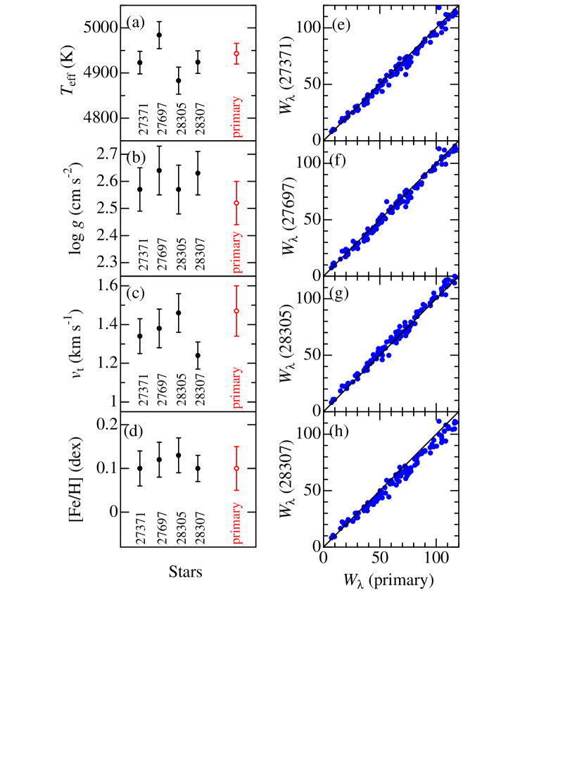
Figure 12: The left-hand panels (a)–(d) illustrate the mutual comparison of the atmospheric parameters ($T_{\rm eff}$, $\log g$, $v_{\rm t}$, and [Fe/H]) of four Hyades giants (HD 27371, 27697, 28305, and 28307; filled circles) and the primary of Capella (open circles). As in Section 4. the attached error bars in panels (a)–(c) indicate the statistical errors, while those in panel (d) are the mean errors. The right-hand panels (e)–(h) show graphical comparisons of the equivalent widths of Fe i and Fe ii lines for the primary of Capella (which we measured in this study based on the disentangled spectra) with those of four Hyades giants (taken from Takeda et al. 2008) having similar atmospheric parameters to the primary: (e) HD 27371, (f) HD 27697, (g) HD 28305, and (h) HD 28307.

The atmospheric parameters ($T_{\rm eff}$, $\log g$, $v_{\rm t}$, and [Fe/H]) of these Hyades giants, which were spectroscopically determined by Takeda et al. (2008) in the same manner as adopted in this study, are graphically compared with those of the primary (cf. Section 4) in Figures 12a–12d, where we can see that they are mostly in accord with each other. Especially, the fact that almost the same metallicity results ([Fe/H] $\sim+0.1$) were derived for all these five stars is meaningful, since the metallicity is expected to be practically equal in this case (unlike other parameters for which small star-to-star difference may be possible). Considering that these parameters were determined from equivalent widths ($W_{\lambda}$) of Fe i and Fe ii lines, we can imagine the similarity of $W_{\lambda}$ for all these stars. Actually, this consistency can be corroborated as demonstrated in Figure 12e–12h, where our $W_{\lambda}$ values of Fe lines for the primary star measured on the disentangled spectrum (cf. “felines.dat”) are compared with those of HD 23371, 27697, 28305, and 28307 (which were taken from tableE2 of Takeda et al. 2008). Consequently, we may conclude also in this respect that the true spectrum has been adequately reproduced by our decomposed spectrum to a practically sufficient precision.

Table 1: Basic information of observed data and relevant radial velocities.

Obs. date	HJD	$\phi$	$\delta V^{\rm hel}$	$V_{\rm p}^{\rm local}$	$V_{\rm p}^{\rm hel}$	$V_{\rm s}^{\rm hel}$	$V_{\rm s}^{\rm local}$	Site/Instrument
(1)	(2)	(3)	(4)	(5)	(6)	(7)	(8)	(9)
2010/04/29	2455315.931	0.8634	$-$19.07	+64.9	+45.83	+10.17	+29.24	Okayama/HIDES
2015/11/30	2457357.170	0.4866	+6.10	$-$7.2	$-$1.10	+57.10	+51.00	Gunma/GAOES
2015/12/18	2457375.282	0.6607	$-$2.54	+17.4	+14.86	+41.14	+43.68	Gunma/GAOES
2016/01/14	2457402.165	0.9191	$-$14.93	+63.2	+48.27	+7.73	+22.66	Gunma/GAOES
2016/02/02	2457421.082	0.1010	$-$21.80	+69.1	+47.30	+8.70	+30.50	Gunma/GAOES
2016/02/15	2457434.002	0.2252	$-$25.17	+57.3	+32.13	+23.87	+49.04	Gunma/GAOES
2016/03/01	2457449.050	0.3698	$-$27.32	+36.0	+8.68	+47.32	+74.64	Gunma/GAOES
2016/03/15	2457463.010	0.5040	$-$27.73	+29.2	+1.47	+54.53	+82.26	Gunma/GAOES
2016/03/16	2457463.959	0.5132	$-$27.75	+29.2	+1.45	+54.55	+82.30	Gunma/GAOES
2016/03/22	2457469.995	0.5712	$-$27.31	+30.3	+2.99	+53.01	+80.32	Gunma/GAOES
2016/03/24	2457471.983	0.5903	$-$27.13	+32.7	+5.57	+50.43	+77.56	Gunma/GAOES
2016/03/25	2457472.978	0.5999	$-$27.03	+33.9	+6.87	+49.13	+76.16	Gunma/GAOES

(1) Observation date (yyyy/mm/dd; in UT). (2) Heliocentric Julian day. (3) Orbital phase, which was calculated with HJD($\phi=0$) = 2450857.21 + 104.02173$E$ ($E$: integer). (4) Heliocentric correction (km s^-1) computed by the “rvcorrect” task of IRAF. (5) Actually observed local topocentric radial velocity (km s^-1) for the primary. (6) Heliocentric radial velocity (km s^-1) for the primary evaluated from $\delta V^{\rm hel}$ and $V_{\rm p}^{\rm local}$. (7) Heliocentric radial velocity (km s^-1) for the secondary evaluated as $56-V_{\rm p}^{\rm hel}$ (km s^-1) based on Equation (1) and Equation (2). (8) Local topocentric radial velocity (km s^-1) for the secondary computed from $\delta V^{\rm hel}$ and $V_{\rm s}^{\rm hel}$. (9) Observing site and used instrument.

Table 2: Evaluated equivalent widths and non-LTE corrections for important lines.

Object	$W_{\lambda}$	$A^{\rm L}$	$A^{\rm N}$	$\Delta^{\rm N}$	Remark
(1)	(2)	(3)	(4)	(5)	(6)
[C i 5380]
primary	16.8	8.501	8.480	$-$0.021
secondary	45.6	8.744	8.701	$-$0.043
Sun	19.9	8.680	8.672	$-$0.008
[Li i 6104]
primary	$\cdots$	$\cdots$	$\cdots$	$\cdots$	undetectable
secondary	20.9	3.338	3.393	+0.055
Sun	$\cdots$	$\cdots$	$\cdots$	$\cdots$	undetectable
[Na i 6161]
primary	124.5	6.878	6.720	$-$0.158
secondary	48.6	6.161	6.090	$-$0.071
Sun	59.0	6.364	6.306	$-$0.058
[Zn i 6362]
primary	41.0	4.826	4.769	$-$0.057
secondary	45.0	4.681	4.651	$-$0.030
Sun	19.4	4.500	4.495	$-$0.005
[Li i 6708]
primary	12.4	0.782	0.988	+0.206
secondary	194.4	3.235	3.176	$-$0.059
Sun	3.1	1.029	1.096	+0.067
[S i 6757]
primary	22.3	7.268	7.240	$-$0.028
secondary	48.0	7.274	7.232	$-$0.042
Sun	20.1	7.207	7.202	$-$0.005
[O i 7774]
primary	53.1	9.139	8.960	$-$0.179	double-line spectrum
secondary	144.6	9.515	9.088	$-$0.427	double-line spectrum
Sun	64.4	8.982	8.879	$-$0.103

(1) Object. (2) Equivalent width (mÅ). See Table 3 of Paper I for the data of the relevant spectral lines. (3) LTE abundance. (4) Non-LTE abundance. (5) Non-LTE correction ($\equiv A^{\rm N}-A^{\rm L}$). (6) Specific remark. Note that $A^{\rm L}$ and $A^{\rm N}$ (logarithmic number abundances) are expressed in the usual normalization of $A({\rm H})=12.00$.

Table 3: Results of relative abundances for the primary and secondary components.

$Z$	Species	[X/H]p	[X/H]s	[Xs/Xp]	$\lambda_{1}$–$\lambda_{2}$ or $N_{\rm p}$/$N_{\rm s}$	Remark
(1)	(2)	(3)	(4)	(5)	(6)	(7)
[Spectrum synthesis analysis]
3	Li	$\cdots$	3.393	$\cdots$	6101–6105	$A$(Li) instead of [Li/H], NLTE
3	Li	0.988	3.176	+2.188	6704–6711	$A$(Li) instead of [Li/H], NLTE
6	C	$-$0.192	+0.029	+0.221	5378.5–5382	NLTE
8	O	+0.006	$\cdots$	$\cdots$	6297–6303
8	O	$-$0.323	$\cdots$	$\cdots$	6361–6365
8	O	+0.081	+0.209	+0.128	7768–7786	NLTE
11	Na	+0.414	$-$0.216	$-$0.630	6157–6164	NLTE
14	Si	+0.169	$-$0.061	$-$0.230	6080–6089
14	Si	+0.175	+0.019	$-$0.156	6297–6303
16	S	+0.038	+0.030	$-$0.008	6751–6760	NLTE
20	Ca	+0.038	$-$0.170	$-$0.208	6101–6105
20	Ca	+0.174	$-$0.251	$-$0.425	6157–6164
21	Sc	$-$0.011	$\cdots$	$\cdots$	6297–6303
22	Ti	+0.376	$-$0.184	$-$0.560	5378.5–5382
22	Ti	$-$0.042	$-$0.163	$-$0.121	6080–6089
23	V	+0.167	$-$0.062	$-$0.229	6080–6089
24	Cr	+0.256	$\cdots$	$\cdots$	6361–6365
26	Fe	+0.214	$-$0.384	$-$0.598	5378.5–5382
26	Fe	+0.029	$-$0.255	$-$0.284	6080–6089
26	Fe	+0.007	$-$0.010	$-$0.017	6101–6105
26	Fe	$-$0.026	$-$0.220	$-$0.194	6157–6164
26	Fe	$-$0.123	$-$0.127	$-$0.004	6297–6303
26	Fe	+0.201	$-$0.094	$-$0.295	6361–6365
26	Fe	+0.057	$-$0.201	$-$0.258	6704–6711
26	Fe	+0.086	$-$0.109	$-$0.195	6751–6760
26	Fe	$-$0.045	$-$0.593	$-$0.548	7768–7786
27	Co	+0.146	$-$0.599	$-$0.745	5378.5–5382
27	Co	+0.210	+0.074	$-$0.136	6080–6089
28	Ni	+0.008	$-$0.306	$-$0.314	6080–6089
28	Ni	+0.086	$-$0.525	$-$0.611	6157–6164
28	Ni	+0.027	$-$0.325	$-$0.352	6361–6365
30	Zn	+0.274	+0.156	$-$0.118	6361–6365	NLTE
[Equivalent width analysis]
14	Si i	$+0.20(\pm 0.12)$	$\cdots$	$\cdots$	17/–
20	Ca i	$+0.16(\pm 0.07)$	$\cdots$	$\cdots$	7/–
21	Sc ii	$+0.02(\pm 0.10)$	$\cdots$	$\cdots$	7/–
22	Ti i	$+0.07(\pm 0.08)$	$\cdots$	$\cdots$	29/–
23	V i	$+0.15(\pm 0.11)$	$\cdots$	$\cdots$	8/–
24	Cr i	$+0.17(\pm 0.09)$	$\cdots$	$\cdots$	14/–
26	Fe i	$+0.10(\pm 0.05)$	$-0.08(\pm 0.08)$	$-0.18(\pm 0.09)$	147/52	Param. determ. by-product
26	Fe ii	$+0.10(\pm 0.06)$	$-0.08(\pm 0.12)$	$-0.18(\pm 0.13)$	16/6	Param. determ. by-product
27	Co i	$+0.08(\pm 0.16)$	$\cdots$	$\cdots$	8/–
28	Ni i	$+0.05(\pm 0.10)$	$-0.10(\pm 0.19)$	$-0.15(\pm 0.13)$	36/10

(1) Atomic number. (2) Element or species. (3) Relative abundance of the primary to the Sun $[\equiv A_{\rm p}({\rm X})-A_{\odot}({\rm X})]$. (4) Relative abundance of the secondary to the Sun $[\equiv A_{\rm s}({\rm X})-A_{\odot}({\rm X})]$. (5) Relative abundance of the secondary to the primary ($[\equiv A_{\rm s}({\rm X})-A_{\rm p}({\rm X})]$). (6) Range (in Å) of spectrum fitting (for spectrum synthesis analysis) or the number of used lines for the primary/secondary (for equivalent width analysis). (7) Specific remark.

Table 4: Published results for the atmospheric parameters, metallicity, and Li abundance of Capella.

Component	$T_{\rm eff}$	$\log g$	$v_{\rm t}$	[Fe/H]	$A$(Li)
(1)	(2)	(3)	(4)	(5)	(6)
[McWilliam (1990)]
Combineda	5270	3.05	$2.0^{b}$	$-0.37^{c}$	$\cdots$
[Pilachowski & Sowell (1992)]
Primary	4800	2.6	2.0	$+0.08^{d}$	0.8
Secondary	5550	2.8	1.0	$-0.08^{d}$	3.0
[Randich et al. (1994)]
Primary	4900	2.6	$\cdots$	$-0.4$	0.6
Secondary	5550	2.8	$\cdots$	$0.0$	3.1
[Fuhrmann (2011)]
Primary	4951	2.68	1.4	$+0.05^{e}$	$\cdots$
Secondary	5672	2.94	1.8	$+0.05^{e}$	$\cdots$
[Torres et al. (2015)]
Primary	4980	2.69	1.48	$-0.03^{f}$	1.08
Secondary	5750	2.94	1.55	$-0.06^{f}$	3.28
[This study]
Primary	4943	2.52	1.47	$+0.10^{g}$	$0.99^{h}$
Secondary	5694	2.88	2.29	$-0.08^{g}$	$3.18^{h}$

(1) Relevant component. (2) Effective temperature (K). (3) Logarithmic surface gravity (cm s^-2/dex). (4) Microturbulent velocity (km s^-1). (5) Fe abundance relative to the Sun (dex). (6) Lithium abundance.

^aPresumably, the apparent line-strengths of the primary component were measured in the double-lined spectrum and simply used as they are.
^bAssumed $v_{\rm t}$.
^cReduced to $-0.20$ if the recent solar abundance of 7.50 is used (cf. Torres to al. 2009).
^d[Ca/H] instead of [Fe/H].
^e[Fe/H]_p=[Fe/H]_s is assumed.
^fResult from Fe i lines.
^gResult from the equivalent widths of Fe i lines as a by-product of atmospheric parameter determination.
^hNon-LTE result from the Li i 6708 line.

References

- (1) Asplund, M., Grevesse, N., Sauval, A. J., & Scott, P. 2009, ARA&A, 47, 481
- (2) Boesgaard, A. M., Budge, K. G. 1988, ApJ, 332, 410
- (3) Eggen, O. J. 1960, MNRAS, 120, 540
- (4) Eggen, O. J. 1972, PASP, 84, 406
- (5) Fuhrmann, K. 2011, ApJ, 742, 42
- (6) Gray, D. F. 1978, Solar Phys., 59, 193
- (7) Gray, D. F. 1982, ApJ, 262, 682
- (8) Gray, D. F. 1988, Lectures on Spectral-Line Analysis: F, G, and K stars (Arva, Ontario, The Publisher)
- (9) Gray, D. F. 2005, The Observation and Analysis of Stellar Photospheres, 3rd ed. (Cambridge, Cambridge University Press)
- (10) Hadrava, P. 1995, A&AS, 114, 393
- (11) Hensberge, H., Ilijić, S., & Torres, K. B. V. 2008, A&A, 482, 1031
- (12) Ilijić, S. 2004, in Spectroscopically and Spatially Resolving the Components of Close Binary Stars, ASP Conf. Ser. Vol. 318, ed. R. W. Hilditch, H. Hensberge, & K. Pavlovski (San Francisco: Astronomical Society of the Pacific), 107
- (13) Kurucz, R. L. 1993, Kurucz CD-ROM, No. 13 (Harvard-Smithsonian Center for Astrophysics)
- (14) Kurucz, R. L., & Bell B. 1995, Kurucz CD-ROM, No. 23 (Cambridge: Smithsonian Astrophysical Observatory)
- (15) Kurucz, R. L., Furenlid, I., Brault, J., & Testerman, L. 1984, Solar Flux Atlas from 296 to 1300 nm (Sunspot, New Mexico: National Solar Observatory)
- (16) Lagarde, N., Decressin, T., Charbonnel, C., Eggenberger, P., Ekström, S., & Palacios, A. 2012, A&A, 543, A108
- (17) McWilliam, A. 1990, ApJS, 74, 1075
- (18) Moultaka, J., Ilovaisky, S. A., Prugniel, P., & Soubiran, C. 2004, PASP, 116, 693
- (19) Pilachowski, C. A., & Sowell, J. R. 1992, AJ, 103, 1668
- (20) Randich, S., Giampapa, M. S., & Pallavicini, R. 1994, A&A, 283, 893
- (21) Sanad, M. R. 2013, Ap&SS, 344, 389
- (22) Simon, K. P., & Sturm, E. 1994, A&A, 281, 286
- (23) Takeda, Y. 1995a, PASJ, 47, 287
- (24) Takeda, Y. 1995b, PASJ, 47, 463
- (25) Takeda, Y. 2008, in The Metal-Rich Universe, eds. G. Israelian & G. Meynet, (Cambridge: Cambridge University Press), 308
- (26) Takeda, Y., et al. 2005a, PASJ, 57, 13
- (27) Takeda, Y., Jeong, G., & Han, I. 2018, PASJ, 70, 8
- (28) Takeda, Y., Honda, S., Ohnishi, T., Ohkubo, M, Hirata, R., & Sadakane, K. 2013, PASJ, 65, 53
- (29) Takeda, Y., Ohkubo, M., & Sadakane, K. 2002, PASJ, 54, 451
- (30) Takeda, Y., Ohkubo, M., Sato, B., Kambe, E., & Sadakane, K. 2005b, PASJ, 57, 27 [Erratum: PASJ, 57, 415]
- (31) Takeda, Y., Sato, B., Kambe, E., Izumiura, H., Masuda, S., & Ando, H. 2005c, PASJ, 57, 109
- (32) Takeda, Y., Sato, B., & Murata, D. 2008, PASJ, 60, 781
- (33) Takeda, Y., Sato, B., Omiya, M., & Harakawa, H. 2015, PASJ, 67, 24
- (34) Takeda, Y., & Tajitsu, A. 2017, PASJ, 69, 74 (Paper I)
- (35) Torres, G., Claret, A., & Young, P. A. 2009, ApJ, 700, 1349
- (36) Torres, G., Claret, A., Pavlovski, K., & Dotter, A. 2015, ApJ, 807, 26
- (37) van Bueren, H. G. 1952, Bull. Astron. Inst. Neth. Supl. Ser. 11, 385
- (38) Zhao, J., Zhao, G., & Chen, Y. 2009, ApJ, 692, L113