Anisotropic Error Estimates of The Linear Virtual Element Method on Polygonal Meshes

Abstract

A refined a priori error analysis of the lowest order (linear) virtual element method (VEM) is developed for approximating a model two dimensional Poisson problem. A set of new geometric assumptions is proposed on the shape regularity of polygonal meshes. A new universal error equation for the lowest order (linear) VEM is derived for any choice of stabilization, and a new stabilization using broken half-seminorm is introduced to incorporate short edges naturally into the a priori error analysis on isotropic elements. The error analysis is then extended to a special class of anisotropic elements with high aspect ratio originating from a body-fitted mesh generator, which uses straight lines to cut a shape regular background mesh. Lastly, some commonly used tools for triangular elements are revisited for polygonal elements to give an in-depth view of these estimates’ dependence on shapes.

65N12, 65N15, 65N30, 46E35

1 Introduction

To present the main idea, consider the weak formulation of the Poisson equation with zero Dirichlet boundary condition in a bounded two-dimensional Lipschitz domain $\Omega$: given an $f\in L^{2}(\Omega)$, find $u\in H_{0}^{1}(\Omega)$ such that

(1.1) $$a(u,v):=(\nabla u,\nabla v)=(f,v)\quad\forall v\in H_{0}^{1}(\Omega).$$

To approximate problem (1.1), $\Omega$ is decomposed into a sequence of polygonal meshes $\{\mathcal{T}_{h},h\in\mathcal{H}\}$. Every $\mathcal{T}_{h}$ consists of a finite number of simple polygons (i.e., open simply connected sets with non-self-intersecting polygonal boundaries). A finite dimensional approximation problem using virtual element method (VEM) is built upon $\mathcal{T}_{h}$. Here the subscript $h$ is the conventional notation for the mesh size: the maximum diameter of polygons in a mesh. The index set $\mathcal{H}$ contains a sequence of $\{h_{n}\}$ and $\lim_{n\to\infty}h_{n}=0$. We are interested in the theoretical proof that the rate of convergence, of a VEM approximation measured under certain norm, is of what order of $h$ and the robustness to the geometry of the polygonal meshes.

VEM was first introduced in [5]. Earlier error analyses of VEM (e.g., [5, 30]) assumed the shape regularity of the mesh, among which the most used assumptions are (1) every polygonal element is star-shaped with a uniform constant and (2) no short edge. VEM splits the approximation (local projections) and stability of the method into two terms. The star-shape assumption is mainly for the approximation property and no short edge is for the stability. Recently some VEM error analyses (see [7, 10]) established the stability of different choices of stabilization without the “no short edge” assumption. Moreover, [17] proposed an alternative way to perform the error analysis through a “virtual” triangulation, the idea of which can be traced back to regular decomposition condition in [11]. Further discussions about geometric conditions on polygons will be featured in Section 3.

Meanwhile in many numerical tests, VEM performs robustly regardless of these seemingly artificial geometric constraints. For instances, it is shown numerically in [6] that VEM converges in the optimal order on Voronoi meshes of which the control vertices are randomly generated. VEM’s convergence is optimal irrelevant to the mesh cuts from the interfaces or fractures (see [8, 18]). In [9], the authors illustrate that, locally on irregular elements, using the orthogonal polynomials, to which the local VEM space is projected, cures the globally instability arising from poor projection matrix conditioning of the conventional-scaled monomials with higher degrees. Similarly in [28, 29], VEM passes the so-called “collapsing polygon test” on certain types of irregular elements with aspect ratio unbounded, when choosing a good set of bases for the polynomials.

The purpose of this paper is to try to further develop the error analyses, inspired by previous references, fit for a broader class of polygonal meshes, thus justifying VEM’s robustness.

First of all, we propose a new stabilization generalizing the scaled nodal difference originally proposed in [38]. The inner product, inducing the broken $1/2$-seminorm on element boundaries, is used as the stabilization. This stabilization is elegantly simple for the linear VEM, which is the scenario of interest in this paper: for $u$, $v$ in the local VEM space in (2.1)

(1.2) $$S_{\mathcal{E}_{K}}(u,v):=\sum_{e\subset\partial K}\bigl{(}u(\bm{b}_{e})-u(\bm{a}_{e})\bigr{)}\bigl{(}v(\bm{b}_{e})-v(\bm{a}_{e})\bigr{)},$$

in which $\bm{b}_{e}$ and $\bm{a}_{e}$ stand for the two end points of an edge $e$. The analysis based on (1.2) matches well with an element boundary integral constraint for the local projection proposed in [2].

To allow a systematic anisotropic error analysis, we then propose a set of more “local-oriented” assumptions inspired by the ones given in [1, 4, 24, 37]. In [37], one assumption on geometrical properties of the polygonal meshes assumes the existence of a shape regular triangle based on each edge $e$ with height $l_{e}$, the size of which is uniform and comparable to the size of the underlying element. This type of assumption however rules out elements with high aspect ratio (anisotropy) and/or short edges. The reason is that an $L^{2}$-weighted trace inequality is used every time, when proving the error estimates involving stabilization with an $h_{e}^{-1}$ factor on the boundary of an element. We shall re-examine various trace inequalities separating the height $l_{e}$ from the length of the edge $h_{e}$, and propose a local height condition. As a result, short edge poses no problem as long as $l_{e}\geq ch_{e}$ for the error analysis on isotropic elements. Notice that the isotropic element class, under the conditions we propose in Section 3, includes a more variety of polygons than the ones under the uniform star-shaped condition.

To be able to apply various trace inequalities on a long edge supporting a short height toward the underlying element, i.e., $l_{e}\ll h_{e}$, we shall embed an anisotropic element into a shape regular agglomerated element, e.g., a square of size $h_{e}$, and apply the trace inequalities in the direction of its shape regular neighboring element. Similar types of embedding can be traced back to [24] for finite element method, in that the convergence is intact if the approximation space on a coarse mesh, which satisfies the maximum angle condition [4], is a subspace of the one defined on a fine but anisotropic mesh. However, for VEM a straightforward subspace argument is not valid, since the VEM spaces are not nested on meshes refined or coarsened from one another.

For the approximation property of the polynomial projection, we propose an alternate shape regularity requirement of the mesh, utilizing the convex hull of a possible nonconvex element. For the interpolation error estimate, as the error measured in $H^{1}$-seminorm is transferred into the combination of that on boundary edges, pairing the edges will bring further cancelation and gives scales in different directions. For interpolation error that stems from the stabilization term, the nodal value difference (1.2) of a linear polynomial (a linear VEM function restricted on boundaries) gives a tangential vector of this edge, which again leads to scales in different directions.

To reveal the possible anisotropy arising from the VEM error analysis while fully exploiting these proof mechanism mentioned above, and to create a presentation easy to follow, we focus on the lowest order (linear) virtual element. We perform the a priori error analysis directly on a weaker norm induced by the bilinear form, by writing out an identity of the error equation. In this way, we avoid to prove the norm equivalence for a stronger $H^{1}$-seminorm, which could possibly introduce more restrictive geometric constraints. Moreover, for the anisotropic error analysis, we restrict ourselves on a special class of polygonal meshes, originally obtained from cutting a rectangular (or a shape regular) background mesh using a set of straight lines (e.g., [18]).

This paper is organized as follows: In Section 2, the basics of VEM are covered, together with a new error equation and an a priori error bound. Section 3 discusses the common geometric assumptions used in polygonal finite element literature, and proposes a new set of assumptions. In Section 4, we present the error analysis on isotropic element based on the new assumptions. In Section 5, we study one class of a possible anisotropic element originated from a body-fitted mesh generator. Lastly in Appendices A-B, we revisit some conventional tools used in finite element, to learn the possible impacts from anisotropy on constants of some widely used inequalities, thus improving the error analysis.

Throughout this paper, for a bounded Lipschitz domain $D$, we opt for the common notation $\left\|\cdot\right\|_{0,D}$ and $(\cdot,\cdot)_{D}$ to denote the $L^{2}$-norm and $L^{2}$-inner product, respectively, and $|\cdot|_{s,D}$ to denote the $H^{s}(D)$-seminorm. When $D=\Omega$ is the whole domain, the subscript $\Omega$ will be omitted. The convex hull of $D$ is denoted as ${\rm conv}(D)$. For any element $K\in\mathcal{T}_{h}$, let $h_{K}={\rm diam}(K)$, $|K|=\operatorname{meas}_{2}(K)$. Let $\mathcal{N}(K):=\{\bm{a}_{1},\bm{a}_{2},\ldots,\bm{a}_{n_{K}}\}$ be the set of vertices on $K$. For any edge $e\subset\partial K$, $h_{e}={\rm diam}(e)=|e|$, $\bm{n}_{e}$ is the unit outward normal vector of $e$ to $K$, and the collection of the edges is $\mathcal{E}_{K}:=\{e\}_{e\subset\partial K}$, the subscripts $e$ and $K$ of which in the context may be omitted for simplicity. $n_{\mathcal{E}_{K}}:=|\mathcal{E}_{K}|$ denotes the total number of edges on the boundary of an element $K$, and it equals $n_{K}$ which is the number of vertices in $K$. For any $L^{1}$-integrable function or vector field $v$, average of $v$ over the domain $D$ is denoted as $\overline{v}^{D}:=|D|^{-1}\int_{D}v$. The tangential derivative for any sufficiently regular function along a continuous curve $\Gamma$ is denoted as $\partial_{\Gamma}v:=\nabla v\cdot\bm{t}_{\Gamma}$, where $\bm{t}_{\Gamma}$ is the unit vector tangential to $\Gamma$ with a given orientation.

For convenience, $x\lesssim y$ and $z\gtrsim w$ are used to represent $x\leq c_{1}y$ and $z\geq c_{2}w$, respectively, where $c_{1}$ and $c_{2}$ are two constants independent of the mesh size $h$. If these constants depend on specific geometric properties of the domain that the underlying quantities are defined on, which may happen, then such dependences, when they exist, shall be stated explicitly. Similarly, $a\eqsim b$ means $a\lesssim b$ and $a\gtrsim b$.

2 VEM

In this section we first introduce the linear virtual element discretization. We then derive a universal error equation for the difference of the VEM approximation to the nodal interpolation for any choice of stabilization, and present an a priori error bound based on the new stabilization.

2.1 Virtual element spaces

The following local VEM space is introduced on a polygonal element $K$:

(2.1) $$V_{K}:=\{v\in H^{1}(K):v|_{\partial K}\in B_{1}(\partial K),\;\Delta v=0\text{ in }K\},$$

where the boundary space $B_{1}(\partial K)$ is defined as

(2.2) $$B_{p}(\partial K):=\{v\in C^{0}(\partial K):v|_{e}\in\mathbb{P}_{p}(e)\text{ for all }e\subset\partial K\},$$

with $\mathbb{P}_{p}(D)$ being the space of the polynomials of degree $\leq p$ defined on a domain $D$.

Using the vertex values as degrees of freedom (d.o.f.), the local space is unisolvent (see [5]), and the canonical interpolation in $V_{K}$ of $v\in H^{1}(K)\cap C^{0}(\overline{K})$ is defined as

(2.3) $$v\mapsto v_{I}\in V_{K}\;\text{ and }\;v_{I}(\bm{a}_{i})=v(\bm{a}_{i}),\quad\forall\bm{a}_{i}\in\mathcal{N}(K).$$

The global $H^{1}$-conforming virtual element space $V_{h}$ for problem (1.1) is then defined as $V_{h}:=\{v\in H_{0}^{1}(\Omega):\;v|_{K}\in V_{K}\}$. The nodal interpolation of a function $v\in H^{1}_{0}(\Omega)\cap C^{0}(\overline{\Omega})$ is denoted by $v_{I}$, where $v_{I}\big{|}_{K}=(v|_{K})_{I}$.

A basis of $V_{K}$ does not have to be represented explicitly in the computation procedure, in which the novelty is that the d.o.f.s are enough to produce an accurate and stable approximation.

2.2 Discretization using virtual element spaces

The local bilinear form $a_{K}(u,v):=(\nabla u,\nabla v)_{K}$ for $u,v\in V_{K}$ cannot be computed exactly, since we do not know $u$ nor $\nabla u$ explicitly. Instead we shall compute an approximation.

Define $\Pi_{K}^{\nabla}:V_{K}\to\mathbb{P}_{1}(K)$ as a local projection in $H^{1}$-seminorm: given $v\in V_{K}$, define $\Pi_{K}^{\nabla}v\in\mathbb{P}_{1}(K)$, which can be computed using the d.o.f. of $v$, such that

(2.4) $$\left(\nabla\bigl{(}v-\Pi_{K}^{\nabla}v\bigr{)},\nabla p\right)_{K}=0,\quad\text{for all }p\in\mathbb{P}_{1}(K).$$

Note that by definition $\nabla\Pi_{K}^{\nabla}v=\overline{\nabla v}^{K}$. The constant kernel space of $\Pi_{K}^{\nabla}$ is then eliminated by an extra constraint in the original VEM paper [5]: $\sum_{i=1}^{n_{K}}\chi_{i}(v-\Pi_{K}^{\nabla}v)=0$. Taking into account the possible anisotropic nature of the element, inspired by [2], we shall use the following constraint

(2.5) $$\int_{\partial K}\left(v-\Pi^{\nabla}_{K}v\right)\,{\rm d}s=0.$$

Henceforth, we shall denote the local projection $\Pi^{\nabla}_{K}$ defined by (2.4)–(2.5) simply by $\Pi$, and when the projection is used in a global term on $\Omega$ or $\mathcal{T}_{h}$, it is piecewise-defined on each element $K$. If in a certain context this notation may give rise to ambiguity, the domain, upon which the projection is performed, will be explicitly mentioned.

Thanks to the local orthogonal projection (2.4) in $H^{1}$-seminorm, the local continuous bilinear form $a_{K}(u,v)$ for $u,v\in V_{K}$ has the following split:

(2.6) $$a_{K}(u,v)=\underbrace{a_{K}\bigl{(}\Pi u,\Pi v\bigr{)}}_{(\mathfrak{c})}+\underbrace{a_{K}\bigl{(}u-\Pi u,v-\Pi v\bigr{)}}_{(\mathfrak{s})}.$$

The $(\mathfrak{c})$ part of (2.6) is now explicitly computable, and is a decent approximation of $a_{K}(u,v)$. Yet it alone does not lead to a stable method.

A stabilization term $S_{K}(\cdot,\cdot)$, matching the $(\mathfrak{s})$ part in (2.6) yet computable, will be added to gain the coercivity of the discretization. Therefore VEM is in fact a family of schemes different in the choice of stabilization terms. Define

(2.7) $$a_{h}(u,v):=\sum_{K\in\mathcal{T}_{h}}a_{K}(\Pi u,\Pi v)+\sum_{K\in\mathcal{T}_{h}}S_{K}\bigl{(}u-\Pi u,v-\Pi v\bigr{)}.$$

A VEM discretization of (1.1) is: find $u_{h}\in V_{h}$ such that

(2.8) $$a_{h}(u_{h},v_{h})=(f,\Pi v_{h})\qquad\forall v_{h}\in V_{h}.$$

Notice that in the right-hand side, we opt to use the $H^{1}$-projection $\Pi v_{h}$ not the $L^{2}$ projection which is not computable for the linear VEM.

The principle of designing a stabilization is two-fold [5]: (1) Consistency. $S_{K}(u,v)$ should vanish when either $u$ or $v$ is in $\mathbb{P}_{1}(K)$. This is always true as in (2.7) the slice operator $(\operatorname{I}-\Pi)$ is applied to the inputs of $S_{K}(\cdot,\cdot)$ beforehand. (2) Stability and continuity. $S_{K}(\cdot,\cdot)$ is chosen so that the following norm equivalence holds

(2.9) $$a(u,u)\lesssim a_{h}(u,u)\lesssim a(u,u)\qquad u\in V_{h}.$$

Thorough error analysis based on (2.9) of several stabilization terms under certain geometric assumption on $\mathcal{T}_{h}$ can be found in [7, 10].

In view of the orthogonal decomposition, i.e., setting $u=v$ in (2.6), and the fact that $u-\Pi u$ is harmonic in $K$, the ideal choice of the stabilization would be the inner product that induces $1/2$-seminorm on $\partial K$: $(u-\Pi u,v-\Pi v)_{\frac{1}{2},\partial K}$. Since the stabilization term then replicates the second term in the split (2.6):

(2.10) $$|u-\Pi u|_{\frac{1}{2},\partial K}=\left\|\nabla(u-\Pi u)\right\|_{0,K}.$$

The identity (2.10) is indeed a definition of the $1/2$-seminorm as the a quotient type norm using a harmonic extension and a trace theorem ([27, Chapter 1, section 8]). We shall choose a computable definition of $1/2$-seminorm, which is equivalent with the one in (2.10): for any function $v$ defined locally on a hyperplane $\Gamma$ in $\mathbb{R}^{2}$,

(2.11) $$\left|v\right|_{\frac{1}{2},\Gamma}^{2}:=\int_{\Gamma}\int_{\Gamma}\frac{|v(\bm{x})-v(\bm{y})|^{2}}{|\bm{x}-\bm{y}|^{2}}\,{\rm d}s(\bm{x})\,{\rm d}s(\bm{y}).$$

Here $\Gamma$ can be the whole $\partial K$ or a connected component being a subset of $\partial K$.

The inner product that induces $1/2$-seminorm on $\partial K$ is further decomposed into a broken one to be used as the stabilization $S_{K}(\cdot,\cdot)$ in (2.7), that is,

(2.12) $$S_{\mathcal{E}_{K}}\bigl{(}u,v\bigr{)}:=\sum_{e\subset\partial K}(u,v)_{\frac{1}{2},e},\qquad u,v\in(\operatorname{I}-\Pi)V_{K},$$

where on an edge $e$

(2.13) $$(u,v)_{\frac{1}{2},e}:=\int_{e}\int_{e}\frac{\bigl{(}u(\bm{x})-u(\bm{y})\bigr{)}\big{(}v(\bm{x})-v(\bm{y})\big{)}}{|\bm{x}-\bm{y}|^{2}}\,{\rm d}s(\bm{x})\,{\rm d}s(\bm{y})$$

For the linear VEM, as the function restricted on each edge is linear, the stabilization term features a very simple formula as follows:

(2.14) $$S_{\mathcal{E}_{K}}(u,v)=\sum_{e\subset\partial K}\bigl{(}u(\bm{b}_{e})-u(\bm{a}_{e})\bigr{)}\bigl{(}v(\bm{b}_{e})-v(\bm{a}_{e})\bigr{)},\quad u,v\in V_{K},$$

in which $\bm{b}_{e}$ and $\bm{a}_{e}$ stand for the two end points of edge $e$. We remark that this stabilization, in the case of linear VEM, is equivalent to a variant of the scaled nodal difference originally proposed in [38] but philosophically different.

Note that by definition, $u\in H^{\frac{1}{2}}(\partial K)$ measured under the broken $1/2$-seminorm induced by $S_{\mathcal{E}_{K}}(\cdot,\cdot)$ is always bounded by its $1/2$-seminorm on the whole boundary:

(2.15) $$|u|_{\frac{1}{2},\mathcal{E}_{K}}^{2}:=S_{\mathcal{E}_{K}}(u,u)=\sum_{e\subset\partial K}|u|_{\frac{1}{2},e}^{2}\leq|u|_{\frac{1}{2},\partial K}^{2}.$$

However, the following inequality of the reverse direction,

(2.16) $$|u|_{\frac{1}{2},\partial K}^{2}\lesssim\sum_{e\subset\partial K}|u|_{\frac{1}{2},e}^{2}=S_{\mathcal{E}_{K}}(u,u),$$

which is usually a key component of the norm equivalence in the traditional VEM error analysis, is in general not true for an arbitrary function in $H^{\frac{1}{2}}(\partial K)$ (e.g., see [23, Theorem 1.5.2.3]). This reverse inequality (2.16) does hold for continuous and piecewise polynomials [14], but the constant hidden in (2.16) depends on the geometry of $K$ and is not fully characterized.

If we follow the classical approach of error analysis of VEM (see, e.g., [5, 7]), by showing the norm equivalence (2.9), geometric conditions on polygons such as shape regularity are indispensable in the proof mechanism. Instead, we shall present a different approach by writing out an error equation.

2.3 Error equation

In this subsection an error equation for $u_{h}-u_{I}$ is derived, where $u_{h}$ is the solution to the VEM approximation problem (2.8) and $u_{I}$ is the nodal interpolation (2.3). A weaker mesh-dependent norm induced by the bilinear form (2.7), with $S_{\mathcal{E}_{K}}(\cdot,\cdot)$ as the stabilization on each element $K$, can be defined as follows and shall be a key ingredient in our analysis:

(2.17) $$\mathopen{|\mkern-2.5mu|\mkern-2.5mu|}u\mathclose{|\mkern-2.5mu|\mkern-2.5mu|}:=a_{h}^{1/2}(u,u)=\left\{\sum_{K\in\mathcal{T}_{h}}\Big{(}\left\|\nabla\Pi u\right\|_{0,K}^{2}+\left|u-\Pi u\right|_{\frac{1}{2},\mathcal{E}_{K}}^{2}\Big{)}\right\}^{1/2}.$$

Lemma 2.1 (a mesh-dependent norm).

$\mathopen{|\mkern-2.5mu|\mkern-2.5mu|}\cdot\mathclose{|\mkern-2.5mu|\mkern-2.5mu|}$ defines a norm on $V_{h}$.

Proof 2.2.

For $u\in V_{K}$, as $u-\Pi u$ is harmonic in $K$, $u-\Pi u$ can be treated as $(u-\Pi u)\big{|}_{\partial K}$’s minimum norm extension in $|\cdot|_{1,K}$. As a result, the following estimate follows from a standard extension theorem (e.g., [31, Theorem 2.5.7], [39, Theorem 4.1]) and the validity of (2.16) for continuous and piecewise polynomials (see [14])

(2.18) $$\|\nabla(u-\Pi u)\|_{0,K}\leq C_{K}\left|u-\Pi u\right|_{\frac{1}{2},\partial K}\lesssim C_{K}\left|u-\Pi u\right|_{\frac{1}{2},\mathcal{E}_{K}}.$$

By the splitting (2.6), the coercivity $\|\nabla u\|^{2}\lesssim a_{h}(u,u)$ then holds $\forall u\in V_{h}$, from which we conclude that $\mathopen{|\mkern-2.5mu|\mkern-2.5mu|}\cdot\mathclose{|\mkern-2.5mu|\mkern-2.5mu|}$ is a norm on $V_{h}\subset H^{1}_{0}(\Omega)$.

Remark 2.3 (norm equivalence).

Indeed (2.18) implies $a(u,u)\lesssim a_{h}(u,u)$ and the equivalence of two definitions of $1/2$-norm, (2.10)–(2.11) implies $a_{h}(u,u)\lesssim a(u,u)$. Therefore we obtain the norm equivalence (2.9) for $u\in V_{h}$. However, the constants involved in the norm equivalence depend on the geometry of $K$ and is not robust to the aspect ratio. Using $\mathopen{|\mkern-2.5mu|\mkern-2.5mu|}\cdot\mathclose{|\mkern-2.5mu|\mkern-2.5mu|}$, a constant-free stability can be obtained. $\Box$

Lemma 2.4 (stability).

Given an $f=-\Delta u\in L^{2}(\Omega)$ for some $u\in H_{0}^{1}(\Omega)$, problem (2.8) is well posed and has the following constant-free stability

(2.19) $$\mathopen{|\mkern-2.5mu|\mkern-2.5mu|}u_{h}\mathclose{|\mkern-2.5mu|\mkern-2.5mu|}=\sup_{v_{h}\in V_{h}}\frac{\bigl{(}f,\Pi v_{h}\bigr{)}}{\mathopen{|\mkern-2.5mu|\mkern-2.5mu|}v_{h}\mathclose{|\mkern-2.5mu|\mkern-2.5mu|}}.$$

Proof 2.5.

First $\mathopen{|\mkern-2.5mu|\mkern-2.5mu|}\cdot\mathclose{|\mkern-2.5mu|\mkern-2.5mu|}$ defines a norm on $V_{h}$, and $\bigl{(}f,\Pi(\cdot)\bigr{)}$ is a linear functional on $V_{h}$, now since $V_{h}$ is finite dimensional, $\bigl{(}f,\Pi(\cdot)\bigr{)}$ is continuous with respect to $\mathopen{|\mkern-2.5mu|\mkern-2.5mu|}\cdot\mathclose{|\mkern-2.5mu|\mkern-2.5mu|}$. Then the identity (2.19) follows from the Riesz representation theorem.

The a priori error analysis shall be carried out for $\mathopen{|\mkern-2.5mu|\mkern-2.5mu|}u_{I}-u_{h}\mathclose{|\mkern-2.5mu|\mkern-2.5mu|}$ by writing out first the following error equation.

Theorem 2.6 (an error equation).

Let $u_{h}$ be the solution to (2.8) and $u_{I}$ be the nodal interpolation defined in (2.3). For any stabilization $S_{K}(\cdot,\cdot)$, the following error representation holds for any $v_{h}\in V_{h}$:

(2.20) $$a_{h}\bigl{(}u_{h}-u_{I},v_{h}\bigr{)} =\sum_{K\in\mathcal{T}_{h}}\left(\nabla\Pi(u-u_{I}),\nabla\Pi v_{h}\right)_{K}$$

$$\;-\sum_{K\in\mathcal{T}_{h}}S_{K}\left(u_{I}-\Pi u_{I},v_{h}-\Pi v_{h}\right)$$

$$\;+\sum_{K\in\mathcal{T}_{h}}{\left\langle\nabla\big{(}u-\Pi u\big{)}\cdot\bm{n},v_{h}-\Pi v_{h}\right\rangle}_{\partial K}.$$

Proof 2.7.

For any $v_{h}\in V_{h}$, using the VEM discretization (2.8) being stable (Lemma 2.4), the underlying PDE $-\Delta u=f$, integration by parts element-wisely, and $\nabla u\cdot\bm{n}$ being continuous across interelement boundaries, we have:

(2.21) $$a_{h}(u_{h},v_{h})-a_{h}(u_{I},v_{h})=-\sum_{K\in\mathcal{T}_{h}}\bigl{(}\Delta u,\Pi v_{h}\bigr{)}_{K}-a_{h}(u_{I},v_{h})$$

$$= \;\sum_{K\in\mathcal{T}_{h}}\bigl{(}\nabla u,\nabla\Pi v_{h}\bigr{)}_{K}-\sum_{K\in\mathcal{T}_{h}}\left\langle\nabla u\cdot\bm{n},\Pi v_{h}\right\rangle_{\partial K}-a_{h}(u_{I},v_{h})$$

$$= \;\sum_{K\in\mathcal{T}_{h}}\left(\nabla\Pi(u-u_{I}),\nabla\Pi v_{h}\right)_{K}-\sum_{K\in\mathcal{T}_{h}}S_{K}\left(u_{I}-\Pi u_{I},v_{h}-\Pi v_{h}\right)$$

$$+\sum_{K\in\mathcal{T}_{h}}\left\langle\nabla u\cdot\bm{n},v_{h}-\Pi v_{h}\right\rangle_{\partial K}.$$

For the last boundary integral term in (2.21), the final error equation (2.20) follows from exploiting the definition of the projection $\Pi=\Pi^{\nabla}_{K}$ in (2.4) and $\Delta\Pi u=0$:

(2.22) $$\left\langle\nabla\Pi u\cdot\bm{n},v_{h}-\Pi v_{h}\right\rangle_{\partial K}=\big{(}\nabla\Pi u,\nabla(v_{h}-\Pi v_{h})\big{)}_{K}=0.$$

We emphasize again that this is an identity for any choice of stabilization terms, under which the solution $u_{h}$ exists for problem (2.8). To get a meaningful convergence result, however, we need a stabilization to be able to control the boundary term $\left\langle\nabla\bigl{(}u-\Pi u\bigr{)}\cdot\bm{n},v_{h}-\Pi v_{h}\right\rangle_{\partial K}$ and meanwhile $u_{I}-\Pi u_{I}$ is of optimal order measured under the seminorm induced by $S_{K}(\cdot,\cdot)$.

Corollary 2.8 (an a priori error bound).

Under the same setting with Theorem 2.6, for the stabilization $S_{\mathcal{E}_{K}}(\cdot,\cdot)$ in (2.14), the following estimate holds:

(2.23) $$\mathopen{|\mkern-2.5mu|\mkern-2.5mu|}u_{h}-u_{I}\mathclose{|\mkern-2.5mu|\mkern-2.5mu|}\lesssim \;\Bigg{\{}\sum_{K\in\mathcal{T}_{h}}\Big{(}\|\nabla\Pi(u-u_{I})\|_{0,K}^{2}+\left|u_{I}-\Pi u_{I}\right|_{\frac{1}{2},\mathcal{E}_{K}}^{2}$$

$$\;+n_{\mathcal{E}_{K}}^{2}\sum_{e\subset\partial K}h_{e}\left\|\nabla\big{(}u-\Pi u\big{)}\cdot\bm{n}\right\|_{0,e}^{2}\Big{)}\Bigg{\}}^{1/2}.$$

Proof 2.9.

Let $v_{h}=u_{h}-u_{I}\in V_{h}$ in the error representation (2.20); applying the Cauchy–Schwarz inequality on the three terms, respectively, yields:

(2.24) $$\mathopen{|\mkern-2.5mu|\mkern-2.5mu|}u_{h}-u_{I}\mathclose{|\mkern-2.5mu|\mkern-2.5mu|}^{2} \leq\sum_{K\in\mathcal{T}_{h}}\left\|\nabla\Pi(u-u_{I})\right\|_{0,K}\left\|\nabla\Pi v_{h}\right\|_{0,K}$$

$$\;+\sum_{K\in\mathcal{T}_{h}}\left|u_{I}-\Pi u_{I}\right|_{\frac{1}{2},\mathcal{E}_{K}}\,\left|v_{h}-\Pi v_{h}\right|_{\frac{1}{2},\mathcal{E}_{K}}$$

$$\;+\sum_{K\in\mathcal{T}_{h}}\sum_{e\subset\partial K}h_{e}^{1/2}\left\|\nabla\big{(}u-\Pi u\big{)}\cdot\bm{n}\right\|_{0,e}\,h_{e}^{-1/2}\left\|v_{h}-\Pi v_{h}\right\|_{0,e}.$$

For the last term above, $\overline{(v_{h}-\Pi v_{h})}^{\partial K}=0$ by the constraint in (2.5). As a result, the error bound follows from the Cauchy–Schwarz inequality, and applying the Poincaré inequality (6.16) on each $e$: recall that $n_{\mathcal{E}_{K}}$ is the number of edges on $\partial K$,

(2.25) $$\sum_{e\subset\partial K}h_{e}^{-1}\left\|v_{h}-\Pi v_{h}\right\|_{0,e}^{2}\leq n_{\mathcal{E}_{K}}^{2}\left|v_{h}-\Pi v_{h}\right|_{\frac{1}{2},\mathcal{E}_{K}}^{2}.$$

In later sections, we shall estimate the three terms in (2.23) based on certain geometric assumptions.

3 Geometric assumptions on polygonal meshes

Some aforementioned error analyses of VEM (see Section 1) are based on the following assumptions on a polygonal mesh $\mathcal{T}_{h}$ in 2-D cases:

1. There exists a real number $\gamma_{1}>0$ such that, for each element $K\in\mathcal{T}_{h}$, it is star-shaped with respect to a disk of radius $\rho_{K}\geq\gamma_{1}h_{K}$.

2. There exists a real number $\gamma_{2}>0$ such that, for each element $K\in\mathcal{T}_{h}$, the distance between any two vertices of $K$ is $\geq\gamma_{2}h_{K}$.

We shall refer to C1 as the $\gamma_{1}$-shape regular condition and C2 as the no short edge condition. Assumption C1 rules out polygons with high aspect ratio, which shall be called as anisotropic element. Equivalently the current error estimate is not robust to the aspect ratio of $K$. Assumption C2 rules out edges with small length which may exists, for example, in polygons of Voronoi tessellation (see [19, 36]). A shape regular polygon may have short edges. A polygon with similar edge lengths may not be shape regular. In particular, triangles/quadrilaterals and tetrahedra satisfying C2 but not C1 are known as slivers, which are problematic in finite element simulations. Yet in practice (see section 1), VEM is robust even when C1, and/or C2 are violated.

Next, we shall propose a set of geometry conditions on polygonal meshes based on the following local quantities for an edge. For an edge $e\subset\partial K$, we choose a local Cartesian coordinate system with $x$-axis aligning with $e$, and positive $y$-direction to be the inward normal of $e$. Define

(3.1) $$\delta_{e}:=\inf\Big{\{}\delta\in\mathbb{R}^{+}:K\cap\big{(}e\times(\delta,+\infty)\big{)}=\varnothing\Big{\}}.$$

For each edge $e\subset\partial K$, an inward height $l_{e}$ associated with edge $e$ can be defined as follows. Let $T(e,l)$ be any triangle with base $e$ and height $l$,

(3.2) $$l_{e}:=\sup\Big{\{}l\in\mathbb{R}^{+}:\exists\,T(e,l)\subset K\cap\big{(}e\times(0,\delta_{e}]\big{)}\Big{\}}.$$

As $K$ is nondegenerate and bounded, $0<\delta_{e}<+\infty$ and $0<l_{e}\leq\delta_{e}$. This height $l_{e}$ measures how far from the edge $e$ one can advance to the interior of $K$ in its inward normal direction. The rectangle $e\times(0,\delta_{e}]$ is used to ensure that the two side angles adjacent to $e$ of triangle $T_{e}=T(e,l_{e})$ are bounded by $\pi/2$. See Figure 1(a).

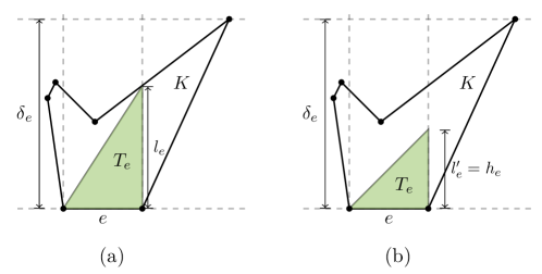
Figure 1: (a) There exists $\gamma>1$ such that $l_{e}\geq\gamma h_{e}$. (b) $T_{e}$ is rescaled with height $l_{e}^{\prime}=h_{e}$.

Remark 3.1.

It would be more meaningful to use notation $h_{e}$ for the height and $l_{e}$ for the length of $e$. However, by the convention of finite element analysis, $h_{e}$ has been reserved for the length. $\Box$

$\mathcal{T}_{h}$ is said to satisfy a certain assumption, if every $K\in\mathcal{T}_{h}$ satisfies that assumption with respect to its constant uniformly as $h\to 0$. An element $K$ is said to be isotropic if the following assumptions (A1-A2) both hold for an element $K$:

• There exists a constant $C_{1}>0$ such that the number of edges $n_{\mathcal{E}_{K}}\leq C_{1}$.

• There exists a constant $\gamma>0$ such that $\forall e\subset\partial K$, $l_{e}\geq\gamma h_{e}$.

Without loss of generality, one can assume that A2 holds with $0<\gamma\leq 1$ when using A2 as a premise of a certain proposition. The reason is that, when A2 holds, one can always rescale the height $l_{e}$ to $l^{\prime}_{e}=\gamma^{\prime}h_{e}$, for any $0<\gamma^{\prime}\leq\gamma$, while a new $T_{e}=T(e,l^{\prime}_{e})$ still satisfies $T_{e}\subset K$. When $\gamma>1$, we can simply set $\gamma^{\prime}=1$ to be the new $\gamma$. See the illustration in Figure 1(b).

Now the anisotropicity of an element $K$ can be characterized by: for one or more edges $e\subset\partial K$, either $l_{e}\ll h_{e}$ or $h_{e}\ll l_{e}$. As the upcoming analysis has shown, the case $h_{e}\ll l_{e}$, i.e., a short edge, is allowed as long as A2 holds. If $h_{e}\ll l_{e}$, one can use the rescaling argument above to obtain a smaller $T_{e}=T(e,l_{e})$ so that $l_{e}\eqsim h_{e}$. In proving the error estimates, $l_{e}\geq\gamma h_{e}$ in A2 is needed when using trace inequalities (Lemmas 4.1, 4.5, and 4.7) or a generalized Poincaré inequality (Lemma 5.6). Assumption A1 is needed, otherwise one can always artificially divide a long edge into short edges to satisfy A2.

The case $l_{e}\ll h_{e}$ is difficult, because the lack of room inside the element makes impossible a smooth extension of functions defined on the boundary. When A2 is not met, it is possible to get a robust error estimate by embedding an anisotropic element in a shape regular one, and separating $h_{e}$ and $l_{e}$ in the refined error analysis.

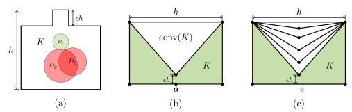
Figure 2: (a) The isotropic $K$ is only star-shaped with respect to $D_{1}$ with radius $\epsilon h$, not to $D_{2}$ or $D_{3}$. (b) The isotropic $K$ has the infamous hourglass shape, but VEM performs robustly on it thanks to the vertex $\bm{a}$ and a bounded number of elements in its convex hull $\mathrm{conv}(K)$. (c) $K$ is anisotropic, edge $e$ violates A2 due to the lack of an extra vertex in the middle; meanwhile A3 is violated if the number of nonconvex wedges grows unbounded as $h\to 0$.

The next requirement for an element $K\in\mathcal{T}_{h}$, Assumption A3, can be also treated as certain shape regularity of the mesh. It is needed for the approximation property, which is originally guaranteed by the star-shaped condition C1. As we do not enforce C1, we provide an alternative way of proving the approximation estimate of the projection in Lemma 4.3. For an element $K$, consider the convex hull $\mathrm{conv}(K)$ of $K$, and obviously $h_{K}=h_{\mathrm{conv}(K)}$. Define $n_{\mathrm{conv}(K)}$ to be the cardinality of the following set:

(3.3) $$n_{\mathrm{conv}(K)}:=\bigl{|}\{K^{\prime}\in\mathcal{T}_{h}:\;K\cap\mathrm{conv}(K^{\prime})\neq\varnothing\}\bigr{|}.$$

• There exists a constant $C_{3}>0$ such that $n_{\mathrm{conv}(K)}\leq C_{3}$.

$n_{\mathrm{conv}(K)}$ represents the number of times an element $K$ has a nonempty intersection with the convex hulls of $K$’s neighboring elements. $\mathcal{T}_{h}$ satisfies A3 if the number of polygons touching every vertex is uniformly bounded, which is true for the most popular polygonal mesh generators (see [19, 36]).

In Section 4, we shall present the error analysis for isotropic elements, and for a special class of anisotropic polygons on which A1 holds but not A2 in Section 5. A3 is required in both scenarios.

In [7, 10], short edges are allowed and integrated into the VEM error analysis by only assuming A1–C1. A2 is inspired by and modified from the uniform height condition $l_{e}\geq\gamma h_{K}$, which is posed as a shape regularity constraint in [37]. One can easily verify that C1 implies A2. When the polygon is star-shaped and $\gamma$-shape regular for a uniform constant $\gamma$, for an edge $e$, the triangle $T_{e}$ can be chosen as the one formed by $e$ and the center of the disk. Although $T_{e}$ may not be shape regular, its height satisfies A2. In our opinion, being shape regular is a local condition near an edge, while being star-shaped requires global information about the whole polygon $K$. In this sense A2 is weaker than C1. For example, a polygon can be isotropic but not uniformly star-shaped; please refer to Figure 2(a), (b), and, in the extreme, the pegasus polygon (winged horses) constructed from M.C Escher’s tessellations in [12].

We now explore more on the geometric properties of isotropic elements.

Lemma 3.2 (scale of the polygon area for isotropic elements).

For an isotropic element $K$, i.e., $K$ satisfies A1-A2, we have the relation

(3.4) $$n_{\mathcal{E}_{K}}^{-2}\gamma\,h_{K}^{2}/2\leq|K|\leq\pi h_{K}^{2}.$$

Proof 3.3.

$|K|\leq\pi h_{K}^{2}$ is true by the definition of the diameter. To prove the lower bound, take the longest edge $e$. By A1, $h_{K}\leq|\partial K|\leq n_{\mathcal{E}_{K}}h_{e}$. We then have $h_{K}^{2}\leq n_{\mathcal{E}_{K}}^{2}h_{e}^{2}\leq(n_{\mathcal{E}_{K}}^{2}/\gamma)l_{e}h_{e}\leq 2(n_{\mathcal{E}_{K}}^{2}/\gamma)|T_{e}|\leq 2(n_{\mathcal{E}_{K}}^{2}/\gamma)|K|$.

For anisotropic polygons, there might exist an edge $e$ such that $l_{e}\ll h_{e}$, i.e., this edge $e$ violates the height condition. The relation between the area and the edge length could be $l_{e}h_{e}/2\leq|K|\ll h_{e}^{2}.$

It is not pragmatic to analyze anisotropic polygons of arbitrary shapes. Later in Section 5, for the ease of presentation, we will restrict ourself to the anisotropic polygons obtained by cutting a square with one straight line, which is a common practice for interface problems (e.g., [18] and the references therein). Depending on the location of the cut, a triangle or quadrilateral may violate A2 as $h\to 0$.

Lemma 3.4 (property of polygons cut from a square).

Let $S$ be a square. Assume that $S=K\cup R$, $\bar{K}\cap\bar{R}$ is a line segment, and $|K|,|R|>0$. Then both $K$ and $R$ satisfy A1 and either $K$ or $R$ is isotropic, i.e., satisfies A1–A2.

Proof 3.5.

Obviously A1 holds with the upper bound $C=5$.

Without loss of generality, it is assumed that $|S|=1$ and $R$ is the polygon with larger area. There are only two cases.

$\bullet$ Case 1: two cut points are on two neighboring sides of $S$ and $R$ is a pentagon.

$\bullet$ Case 2: two cut points are on the opposite sides of $S$ and $R$ is a trapezoid and could be degenerate to a triangle when the cut forms the diagonal of $S$.

For any edge $e$ of $R$, one can choose the farthest vertex, which has the largest distance to this edge to form the triangle $T_{e}$, and the height $l_{e}$ is the distance. The maximum angle of $T_{e}$ is bounded by $\pi/2$. For A2: (1) When the edge $e$ is also on the boundary of the square, the height $l_{e}$ is the distance of the vertex to the edge $\geq 1/2$ as $R$ is assumed to have the larger area. (2) For the cut edge, the largest distance is $\geq\sqrt{2}/2$ in the pentagon case, and $\geq 2/\sqrt{5}$ for the trapezoid.

4 Error analysis for isotropic elements

In this section we shall provide optimal order error estimate for linear VEM approximation on isotropic elements, i.e., polygons satisfying Assumption A1–A2–A3.

We first present an interpolation error estimate. Thanks to the error bound (2.23), we do not need to estimate $\left\|\nabla(u-u_{I})\right\|$ but its projection $\left\|\nabla\Pi(u-u_{I})\right\|$, which can be transferred to the element boundary through integration by parts. The interpolation error $u-u_{I}$ is well understood along the boundary. A2 gives room to trace inequalities to lift the estimate to the interior.

Lemma 4.1 (a projection-type error estimate for the interpolation on isotropic polygons).

If $K$ satisfies A1–A2 with $0<\gamma\leq 1$, then for any $u\in H^{2}(K)$,

(4.1) $$\left\|\nabla\Pi(u-u_{I})\right\|_{0,K}\lesssim n_{\mathcal{E}_{K}}\gamma^{-1}\,h_{K}|u|_{2,K}.$$

Proof 4.2.

Let $q=\Pi(u-u_{I})\in\mathbb{P}_{1}(K)$, then by the definition of $\Pi$ in (2.4):

(4.2) $$\left(\nabla\Pi(u-u_{I}),\nabla q\right)_{K}=\left(\nabla(u-u_{I}),\nabla q\right)_{K}=\sum_{e\subset\partial K}(u-u_{I},\nabla q\cdot\bm{n})_{e}.$$

Being restricted to one edge, $(u-u_{I})|_{e}$ can be estimated by the standard interpolation error estimate in fractional Sobolev norm (see e.g. [20, Section 8, example 3] and [22]): $\left\|u-u_{I}\right\|_{0,e}\lesssim h_{e}^{3/2}|u|_{\frac{3}{2},e}$. For the edge $e$ satisfying the A1–A2, use trace inequality (6.3) in Lemma 6.2 on $\nabla u$ component-wisely for the term $|u|_{\frac{3}{2},e}$,

(4.3) $$(u-u_{I},\nabla q\cdot\bm{n})_{e}\leq\left\|u-u_{I}\right\|_{0,e}\left\|\nabla q\cdot\bm{n}\right\|_{0,e}\lesssim\;h_{e}^{3/2}|u|_{\frac{3}{2},e}\,|\nabla q|\,h_{e}^{1/2}$$

$$\lesssim \;\frac{1}{\sqrt{\gamma}}\frac{h_{e}}{|K|^{1/2}}\,h_{e}|u|_{2,K}\,|\nabla q||K|^{1/2}\,\lesssim\;\frac{1}{\gamma}h_{K}|u|_{2,K}\left\|\nabla q\right\|_{0,K},$$

wherein the last step, we have used $h_{e}\leq h_{K}$ and $h_{e}^{2}/|K|\lesssim\gamma^{-1}l_{e}h_{e}/|K|\leq\gamma^{-1}$ implied by A2. Summing up on each $e$ and canceling $\left\|\nabla q\right\|_{0,K}$, we get (4.1).

In view of the proof, the error contribution is actually proportional to the edge length and thus a short edge is not an issue. A2 is required to apply the trace inequalities, as well as the ratio $h_{e}/|K|^{1/2}$ being bounded. A1 is needed in that the error estimate in (4.3) is summed over all edges. For anisotropic elements, a long edge may only support a very short height moving inward to the interior of $K$ and thus $|K|\ll h_{e}^{2}$, needing a more delicate analysis detailed in section 5. We now move to the estimate of the projection error $\nabla(u-\Pi u)$.

Lemma 4.3 (error estimate for the projection).

Let $\mathrm{conv}(K)$ be the convex hull of $K$, then for any $u\in H^{2}({\rm conv}(K))$, the following error estimate holds:

(4.4) $$\left\|\nabla\bigl{(}u-\Pi u\bigr{)}\right\|_{0,K}\leq\frac{h_{K}}{\pi}|u|_{2,\mathrm{conv}(K)}.$$

Proof 4.4.

As $\nabla\Pi u=\overline{\nabla u}^{K}$ is the best constant approximation in $L^{2}(K)$-norm:

$$\left\|\nabla\bigl{(}u-\Pi u\bigr{)}\right\|_{0,K}\leq\big{\|}\nabla u-\overline{\nabla u}^{\mathrm{conv}(K)}\big{\|}_{0,K}\leq\big{\|}\nabla u-\overline{\nabla u}^{\mathrm{conv}(K)}\big{\|}_{0,\mathrm{conv}(K)},$$

then the Poincaré inequality in Lemma 6.7 on the convex set $\mathrm{conv}(K)$, together with the fact that $h_{K}=h_{\mathrm{conv}(K)}$, implies (4.4).

The approximation result (4.4) is usually established using the average over the contained disk for a star-shaped element and thus depends on the so-called chunkiness parameter in C1 (the diameter over the largest radius of the disk with respect to which the domain is star-shaped). Here we use the convexity of $\mathrm{conv}(K)$ as it does not require any shape regularity of the element $K$.

Lemma 4.5 (error estimate for the normal derivative of projection on isotropic polygons).

If $K$ satisfies A1–A2 with $0<\gamma\leq 1$, then for any $u\in H^{2}(\mathrm{conv}(K))$, on each $e\subset\partial K$:

(4.5) $$h_{e}^{1/2}\left\|\nabla\bigl{(}u-\Pi u\bigr{)}\cdot\bm{n}\right\|_{0,e}\lesssim\gamma^{-1/2}h_{K}|u|_{2,\mathrm{conv}(K)}.$$

Proof 4.6.

With A1–A2, we can apply the weighted trace inequality (6.8) in Appendix A, and estimate (4.4) to get

(4.6) $$h_{e}^{1/2}\left\|\nabla\bigl{(}u-\Pi u\bigr{)}\cdot\bm{n}\right\|_{0,e}\lesssim{\gamma^{-\frac{1}{2}}}\left(\left\|\nabla\bigl{(}u-\Pi u\bigr{)}\right\|_{0,K}+h_{e}|u|_{2,K}\right)\lesssim\gamma^{-\frac{1}{2}}h_{K}|u|_{2,\mathrm{conv}(K)}.$$

!

Lastly, the broken $1/2$-seminorm term in (2.23) on each edge which again can be easily estimated using a trace inequality as in the traditional finite element analysis.

Lemma 4.7 (error estimate for the stabilization on isotropic polygons).

If $K$ satisfies A1–A2 with $0<\gamma\leq 1$, then for any $u\in H^{2}(\mathrm{conv}(K))$, on each $e\subset\partial K$

(4.7) $$|u_{I}-\Pi u_{I}|_{\frac{1}{2},e}\lesssim n_{\mathcal{E}_{K}}\gamma^{-3/2}\,h_{K}|u|_{2,\mathrm{conv}(K)}.$$

Proof 4.8.

Split $u_{I}-\Pi u_{I}=(u_{I}-\Pi u)+(\Pi u-\Pi u_{I})$. For the second term, one can use the trace inequality (6.3) and the interpolation error estimate (4.1)

(4.8) $$\left|\Pi u-\Pi u_{I}\right|_{\frac{1}{2},e}\lesssim\gamma^{-\frac{1}{2}}\left\|\nabla(\Pi u-\Pi u_{I})\right\|_{0,K}\lesssim n_{\mathcal{E}_{K}}\gamma^{-\frac{3}{2}}\,h_{K}|u|_{2,K}.$$

For the first term $\left|u_{I}-\Pi u\right|_{\frac{1}{2},e}$, since $u_{I}$ and $u$ match at the vertices $\bm{a}_{e}$ and $\bm{b}_{e}$ of $e$, one has

(4.9) $$(u_{I}-\Pi u)\Big{|}_{\bm{a}_{e}}^{\bm{b}_{e}}=(u-\Pi u)\Big{|}_{\bm{a}_{e}}^{\bm{b}_{e}}=\int_{e}\partial_{e}(u-\Pi u)\,{\rm d}s.$$

Thus by the Cauchy–Schwarz inequality and because $u_{I}$ is linear on $e$:

(4.10) $$\left|u_{I}-\Pi u\right|_{\frac{1}{2},e}=\left|(u_{I}-\Pi u)\big{|}_{\bm{a}_{e}}^{\bm{b}_{e}}\right|\leq h_{e}^{1/2}\left\|\partial_{e}(u-\Pi u)\right\|_{0,e}.$$

Applying the trace inequality (6.8) and the estimate (4.4) then yields the lemma:

(4.11) $$h_{e}^{1/2}\left\|\partial_{e}(u-\Pi u)\right\|_{0,e}\lesssim\gamma^{-\frac{1}{2}}\left(\left\|\nabla(u-\Pi u)\right\|_{0,K}+h_{e}|u|_{2,K}\right)\lesssim\gamma^{-\frac{1}{2}}h_{K}|u|_{2,\mathrm{conv}(K)}.$$

We now summarize the convergence result on isotropic meshes as follows.

Theorem 4.9 (a priori convergence result for VEM on isotropic meshes).

Assume that $\mathcal{T}_{h}$ satisfies A1–A2–A3, and that the weak solution $u$ to problem (1.1) satisfies the regularity result $u\in H^{2}(\Omega)$; then the following a priori error estimate holds for the solution $u_{h}$ to problem (2.8) with constant dependencies $C_{\gamma}:=1/\min\{\gamma,1\}$ with $\gamma$ being the uniform lower bound for each edge in each $K\in\mathcal{T}_{h}$ satisfying A2, $C_{\mathcal{E}}:=\max_{K\in\mathcal{T}_{h}}n_{\mathcal{E}_{K}}$, and $C_{\omega}:=\max_{K\in\mathcal{T}_{h}}n_{{\rm conv}(K)}$ with $n_{\mathrm{conv}(K)}$ in (3.3):

(4.12) $$\mathopen{|\mkern-2.5mu|\mkern-2.5mu|}u-u_{h}\mathclose{|\mkern-2.5mu|\mkern-2.5mu|}\lesssim C_{\gamma}^{3/2}C_{\mathcal{E}}^{3/2}C_{\omega}^{1/2}\,h\,|u|_{2,\Omega}.$$

Proof 4.10.

First of all, we apply the Stein’s extension theorem ([35, Theorem 6.5]) to $u\in H^{2}(\Omega)\cap H^{1}_{0}(\Omega)$ to obtain $Eu\in H^{2}(\mathbb{R}^{2})$, $Eu|_{\Omega}=u|_{\Omega}$, and $|Eu|_{2,\mathbb{R}^{2}}\leq C(\Omega)|u|_{2,\Omega}$. With this extension $Eu\in H^{2}\big{(}\mathrm{conv}(K)\big{)}$ for any $K\in\mathcal{T}_{h}$.

Using Corollary 2.8, Lemmas 4.1, 4.5, 4.7, assuming $\mathcal{T}_{h}$ satisfies A2 with $0<\gamma\leq 1$, and the fact that the integral on the overlap $\mathrm{conv}(K)\cap\mathrm{conv}(K^{\prime})$ (when $\partial K\cap\partial K^{\prime}\neq\varnothing$) is repeated $n_{\mathrm{conv}(K)}$ times by A3, we obtain

(4.13) $$\mathopen{|\mkern-2.5mu|\mkern-2.5mu|}u_{I}-u_{h}\mathclose{|\mkern-2.5mu|\mkern-2.5mu|}^{2} \lesssim\sum_{K\in\mathcal{T}_{h}}(n_{\mathcal{E}_{K}}^{2}\gamma^{-2}+n_{\mathcal{E}_{K}}^{3}\gamma^{-3}+n_{\mathcal{E}_{K}}^{3}\gamma^{-1})h_{K}^{2}|Eu|_{2,\mathrm{conv}(K)}^{2}$$

$$\lesssim C_{\omega}C_{\mathcal{E}}^{3}\gamma^{-3}h^{2}|Eu|_{2,\mathrm{conv}(\Omega)}^{2}\lesssim C_{\omega}C_{\mathcal{E}}^{3}\gamma^{-3}h^{2}|u|_{2,\Omega}^{2}.$$

By the triangle inequality and Young’s inequality, it suffices to estimate $\mathopen{|\mkern-2.5mu|\mkern-2.5mu|}u-u_{I}\mathclose{|\mkern-2.5mu|\mkern-2.5mu|}$:

(4.14) $$\mathopen{|\mkern-2.5mu|\mkern-2.5mu|}u-u_{I}\mathclose{|\mkern-2.5mu|\mkern-2.5mu|}^{2}\lesssim\sum_{K\in\mathcal{T}_{h}}\left(\left\|\nabla\Pi(u-u_{I})\right\|_{0,K}^{2}+\left|u_{I}-\Pi u_{I}\right|_{\frac{1}{2},\mathcal{E}_{K}}^{2}+\left|u-\Pi u\right|_{\frac{1}{2},\mathcal{E}_{K}}^{2}\right).$$

The first two terms above have been dealt with in Lemmas 4.1 and 4.7. For the third term, by A1–A2 and Lemma 6.2:

(4.15) $$\left|u-\Pi u\right|_{\frac{1}{2},\mathcal{E}_{K}}^{2}=\sum_{e\subset\partial K}\left|u-\Pi u\right|_{\frac{1}{2},e}^{2}\lesssim n_{\mathcal{E}_{K}}\gamma^{-1}\left\|\nabla(u-\Pi u)\right\|_{0,K}^{2},$$

and the theorem follows from using the projection estimate (4.4) on $\left\|\nabla(u-\Pi u)\right\|_{0,K}$.

In light of the approximation error estimates (4.4) and (4.12), the estimate

(4.16) $$\left(\sum_{K\in\mathcal{T}_{h}}\left\|\nabla u-\nabla\Pi u_{h}\right\|_{0,K}^{2}\right)^{1/2}\lesssim h|u|_{2,\Omega}$$

can then be obtained from the triangle inequality. Although $u_{h}$ is not explicitly known, the computable discontinuous piecewise linear polynomial $\Pi u_{h}$ is an optimal order approximation of $u$ in the discrete $H^{1}$-seminorm.

Remark 4.11 (other choices of stabilization).

We remark here that the analyses used in this section apply to other types of stabilizations analyzed in [5, 7, 10, 37, 38]:

• $L^{2}$-type $S_{K}(u,v)=\sum_{e\subset\partial K}h_{e}^{-1}(u,v)_{e}$,

• d.o.f.-type $S_{K}(u,v)=\sum_{\bm{a}\in\mathcal{N}_{K}}u(\bm{a})v(\bm{a})$,

• tangential derivative-type $S_{K}(u,v)=\gamma_{K}\sum_{e\subset\partial K}(\partial_{e}u,\partial_{e}v)_{e}$.

In [37], no short edge condition is imposed, because an $L^{2}$-weighted trace inequality is used for the $L^{2}$-type stabilization with an $h_{e}^{-1}$-weight. In our approach, the Poincaré-type inequality (2.25) allows short edges in an element without further modifying the $h_{e}^{-1}$ weight. Replacing weight $h_{e}^{-1}$ with $h_{K}^{-1}$ in these stabilization terms is also allowed if an irregular polygon can be embedded into another shape regular one (see Section 5). $\Box$

Remark 4.12 (removal of the $\log$ factor).

Comparing with the analyses in [7, 10] by bridging the VEM bilinear form $a_{h}(\cdot,\cdot)$ with $|\cdot|_{1,K}$ through norm equivalences, we opt to work on a weaker norm $\mathopen{|\mkern-2.5mu|\mkern-2.5mu|}\cdot\mathclose{|\mkern-2.5mu|\mkern-2.5mu|}=a^{1/2}_{h}(\cdot,\cdot)$ to avoid introducing some extra geometric constraints for the equivalence between $|\cdot|_{\frac{1}{2},\partial K}$ and the stabilization. The benefit of this is that the analysis based on the broken $1/2$-seminorm $|\cdot|_{\frac{1}{2},\mathcal{E}_{K}}$ does not pay the $\log\big{(}h_{K}/\min_{e\subset\partial K}h_{e}\big{)}$ factor. This log factor is unavoidable as well for the d.o.f.-type stabilization since the proof demands certain equivalence between $|\cdot|_{\frac{1}{2},\partial K}$ and $\left\|\cdot\right\|_{\infty,\partial K}$. The introduction of $|\cdot|_{\frac{1}{2},\mathcal{E}_{K}}$ evades this problem, as Corollary 6.14 further demonstrates that $\left\|v_{h}\right\|_{\infty,\partial K}\eqsim|v_{h}|_{\frac{1}{2},\mathcal{E}_{K}}$ if $v_{h}\in V_{K}$ and $\overline{v}_{h}^{\partial K}=0$. $\Box$

The local error analysis in this section is based on A1–A2–A3. In the subsequent section we shall generalize the anisotropic analysis for triangles to a special class of anisotropic polygons with A2 violated.

5 Error analysis for a special class of anisotropic elements

In this section we shall present error analysis for a special class of anisotropic elements, which are obtained by cutting a uniform grid consisting of squares of size $h$. The present approach could be possibly extended to other shape regular meshes; see Remark 5.13.

Henceforth the polygonal mesh can be anisotropic in the sense that it only satisfies A1 but there may exist elements not satisfying A2. Namely there is a long edge with a short height in such an element, so the trace inequalities and Poincaré inequalities cannot be applied freely. We shall embed an anisotropic element into a shape regular element, e.g. a square of size $h$, and apply trace inequalities on the shape regular element. We shall also make use of the cancelation of contributions from different boundary edges to bound the interpolation error and the stabilization error.

5.1 Interpolation error estimates

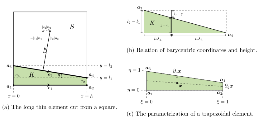
Figure 3: The anisotropic element setting used in Lemma 5.1, 5.6, 5.8, and 6.17.

Lemma 5.1 (a projection-type error estimate for the interpolation in a cut element).

Assume $K$ is obtained by cutting a square $S$; then

(5.1) $$\left\|\nabla\Pi(u-u_{I})\right\|_{0,K}\lesssim h_{K}|u|_{2,S},\qquad u\in H^{2}(S).$$

Proof 5.2.

We process as before (cf. (4.1)), by letting $q=\Pi(u-u_{I})$ to obtain

(5.2) $$\left\|\nabla\Pi(u-u_{I})\right\|_{0,K}=\sum_{e\subset\partial K}(u-u_{I},\nabla q\cdot\bm{n})_{e}.$$

If $K$ is a right triangle, the error analysis can be applied for triangles satisfying the maximum angle condition [4]. If $K$ is a pentagon, $K$ is isotropic by Lemma 3.4 and thus the estimate on isotropic polygons can be applied. So here $K$ is assumed to a right trapezoid, of which one side is aligned with $S$ (see Figure 3(a)), and $l_{2}>l_{1}$ and $l_{1}$ could vanish in which case the right trapezoid is degenerated to a triangle. For edges $e_{2}$ and $e_{4}$, A1–A2 holds and thus proofs in Lemma 4.1 can be applied, while for edge $e_{1}$ and $e_{3}$, $l_{e}\ll h_{e}$.

By parametrizing using $0\leq x\leq h$, the edge $e_{1}$ from $\bm{a}_{1}$ to $\bm{a}_{2}$: $\bm{r}_{1}=\langle x,0\rangle$, and $e_{3}$ from $\bm{a}_{3}$ to $\bm{a}_{4}$: $\bm{r}_{3}=\langle x,l_{1}-x\tan\theta\rangle$ (where $\cos\theta=-\bm{n}_{1}\cdot\bm{n}_{3}$), and decomposing the outer unit normal to $e_{3}$ as $\bm{n}_{3}=-\bm{n}_{1}\cos\theta+\bm{n}_{2}\sin\theta$, the boundary integrals on $e_{1}$ and $e_{3}$ can be written as

(5.3) $$\;(u-u_{I},\nabla q\cdot\bm{n})_{e_{1}}+(u-u_{I},\nabla q\cdot\bm{n})_{e_{3}}$$

$$= \underbrace{\int_{0}^{h}\left[(u-u_{I})(\bm{r}_{1})-(u-u_{I})(\bm{r}_{3})\right]\nabla q\cdot\bm{n}_{1}\,{\rm d}x}_{(\flat)}+\underbrace{\int_{0}^{h}(u-u_{I})(\bm{r}_{3})\nabla q\cdot\bm{n}_{2}\tan\theta\,{\rm d}x}_{(\natural)}.$$

Before moving into the details, we use a special case: $K$ is a rectangle with side $h$ and height $l$ to explain briefly the cancelation technique. In this case, $\bm{n}_{3}=-\bm{n}_{1}$ and thus the term $(\natural)$ disappears. The interpolation error $u-u_{I}$ along the horizontal edges $\bm{e}_{1}$ and $\bm{e}_{3}$ is of order $h$ and the difference $(u-u_{I})(\bm{r}_{1})-(u-u_{I})(\bm{r}_{3})$ is of order $l$. So a refined scale $lh$ instead of $h^{2}$ is obtained.

For a general trapezoid, $\bm{e}_{3}$ may not be parallel to $\bm{e}_{1}$. But the factor $h\tan\theta=l_{2}-l_{1}$ weighing like a short edge. The integral $(\natural)$ above can be dealt with using a similar argument with (4.3):

(5.4) $$|(\natural)|\lesssim h(l_{2}-l_{1})|u|_{\frac{3}{2},e_{3}}|\nabla q|\lesssim|K|^{1/2}|u|_{2,S}\left\|\nabla q\right\|_{0,K}.$$

The integral $(\flat)$ in (5.3) is now the focus. For a point $\bm{r}_{1}=\langle x,0\rangle\in e_{1}$, the barycentric coordinate $\lambda_{i}(\bm{r}_{1})$ ($i=1,2$) are positive numbers satisfying $\langle x,0\rangle=\lambda_{1}(x,0)\bm{a}_{1}+\lambda_{2}(x,0)\bm{a}_{2}$. Using the fundamental theorem of calculus, it is straightforward to arrive at the following error representation on $e_{1}$:

(5.5) $$(u-u_{I})(\bm{r}_{1})=\lambda_{1}(x,0)\int^{x}_{0}\partial_{x}u(t,0)\,{\rm d}t-\lambda_{2}(x,0)\int^{h}_{x}\partial_{x}u(t,0)\,{\rm d}t.$$

Similarly on $e_{3}$, for a point $\bm{r}_{3}=\langle x,y\rangle\in e_{3}$, introduce the barycentric coordinate $\lambda_{i}(\bm{r}_{3})$ ($i=3,4$) satisfying $\langle x,y\rangle=\lambda_{3}(x,y)\bm{a}_{3}+\lambda_{4}(x,y)\bm{a}_{4}$. We have the error representation on $e_{3}$:

(5.6) $$(u-u_{I})(\bm{r}_{3})=\lambda_{3}(\bm{r}_{3})\int_{\bm{a}_{3}}^{\bm{r}_{3}}\partial_{t}u\,{\rm d}t-\lambda_{4}(\bm{r}_{3})\int_{\bm{r}_{3}}^{\bm{a}_{4}}\partial_{t}u\,{\rm d}t.$$

To be able to cancel with terms in (5.5), we further decompose the line integral along $\bm{e}_{3}$ into coordinate directions:

(5.7) $$(u-u_{I})(\bm{r}_{3}) =-\lambda_{3}(x,y)\int^{l_{2}}_{y}\partial_{y}u(x,\tau)\,{\rm d}\tau+\lambda_{3}(x,y)\int^{x}_{0}\partial_{x}u(t,l_{2})\,{\rm d}t$$

$$\quad+\lambda_{4}(x,y)\int^{y}_{l_{1}}\partial_{y}u(x,\tau)\,{\rm d}\tau-\lambda_{4}(x,y)\int^{h}_{x}\partial_{x}u(t,l_{1})\,{\rm d}t.$$

It follows from the fact that $\lambda_{1}(x,0)=\lambda_{3}(x,y)$ and $\lambda_{2}(x,0)=\lambda_{4}(x,y)$:

(5.8) $$(u-u_{I})(\bm{r}_{1})-(u-u_{I})(\bm{r}_{3})$$

$$= \;\underbrace{\lambda_{1}(x,0)\int^{x}_{0}\big{[}\partial_{x}u(t,0)-\partial_{x}u(t,l_{2})\big{]}\,{\rm d}t+\lambda_{2}(x,0)\int^{h}_{x}\big{[}\partial_{x}u(t,l_{1})-\partial_{x}u(t,0)\big{]}\,{\rm d}t}_{(\dagger)}$$

$$+\underbrace{\lambda_{3}(x,y)\int^{l_{2}}_{y}\partial_{y}u(x,\tau)\,{\rm d}\tau-\lambda_{4}(x,y)\int^{y}_{l_{1}}\partial_{y}u(x,\tau)\,{\rm d}\tau}_{(\ddagger)}.$$

Assuming $l_{1}\neq l_{2}$, otherwise $(\ddagger)=0$, applying the mean value theorem on both integrals in $(\ddagger)$, there exists $\xi_{2}\in(y,l_{2})$, and $\xi_{1}\in(l_{1},y)$ such that

(5.9) $$(\ddagger) =\lambda_{3}(x,y)(l_{2}-y)\partial_{y}u(x,\xi_{2})-\lambda_{4}(x,y)(y-l_{1})\partial_{y}u(x,\xi_{1})$$

$$=\frac{(l_{2}-y)(y-l_{1})}{l_{2}-l_{1}}\int^{\xi_{2}}_{\xi_{1}}\partial_{yy}u(x,\tau)\,{\rm d}\tau\leq\frac{l_{2}-l_{1}}{4}\int^{l_{2}}_{l_{1}}|\partial_{yy}u(x,y)|\,{\rm d}y.$$

wherein the second step the geometric meaning of barycentric coordinates (see Figure 3(b)) is used:

(5.10) $$\frac{\lambda_{3}(x,y)}{y-l_{1}}=\frac{\lambda_{4}(x,y)}{l_{2}-y}=\frac{1}{l_{2}-l_{1}}.$$

For $(\dagger)$, an estimate can be obtained as follows:

(5.11) $$\bigl{|}(\dagger)\bigr{|} \leq{\left|\lambda_{1}(x,0)\int^{x}_{0}\int^{l_{2}}_{0}\partial_{xy}u(t,\tau)\,{\rm d}\tau dt\right|}+{\left|\lambda_{2}(x,0)\int^{h}_{x}\int^{l_{1}}_{0}\partial_{xy}u(t,\tau)\,{\rm d}\tau dt\right|}$$

$$\leq\left\|\partial_{xy}u\right\|_{0,S}h^{1/2}l_{1}^{1/2}+\left\|\partial_{xy}u\right\|_{0,S}h^{1/2}l_{2}^{1/2}\lesssim|K|^{1/2}|u|_{2,S}.$$

By the estimate in (5.9), together with (5.11), the integral $(\flat)$ in (5.3) can be estimated as follows:

(5.12) $$|(\flat)|\leq \;\int^{h}_{0}|(\dagger)|\,|\nabla q|\,\,{\rm d}x+\frac{l_{2}-l_{1}}{4}\int^{h}_{0}\int^{l_{2}}_{l_{1}}|\partial_{yy}u(x,y)|\,|\nabla q|\,{\rm d}y\,{\rm d}x$$

$$\lesssim \;\;h|K|^{1/2}|\nabla q|\,|u|_{2,S}+\frac{l_{2}-l_{1}}{4}\left(\int_{K}|\partial_{yy}u(x,y)|^{2}\,{\rm d}x\,{\rm d}y\right)^{\frac{1}{2}}|K|^{1/2}|\nabla q|,$$

which can be bounded by $h_{K}|u|_{2,S}\left\|\nabla q\right\|_{0,K}$. In summary, we have proved the following inequality and (5.1) is obtained by canceling $\left\|\nabla q\right\|_{0,K}$ on both sides:

(5.13) $$\left\|\nabla\Pi(u-u_{I})\right\|_{0,K}^{2}\lesssim h_{K}|u|_{2,S}\left\|\nabla q\right\|_{0,K}.$$

Remark 5.3 (generalization to certain anisotropic polygons).

The proof of the interpolation estimate is not restricted to anisotropic quadrilaterals. Heuristically speaking, if there is a long edge $e$ (which can be $e_{1}$ in Figure 3(a)) that supports a short height $l_{e}$ toward the interior of an anisotropic element $K$. Meanwhile if there exists another long edge ($e_{3}$ in the aforementioned case) on $\partial K$ pairing with this long edge, then the cancelation will occur for terms $(u-u_{I},\nabla q\cdot\bm{n})_{e_{i}}$ ($i=1,3$) among the ones in (5.2). Even on quadrilaterals, our analysis on VEM relaxes the stringent constraints imposed on isoparametric elements for anistropic quadrilaterals (cf. [1] and the references therein). However, a precise characterization of the class of anisotropic elements for which this analysis can be applied seems difficult. For example, the same cancelation argument can be generalized to the element in Figure 2(b), but not to the element in Figure 2(a). The existence of three long edges in Figure 2(a) forbids a straightforward pairing and cancelation trick to yield the desirable estimate. $\Box$

Figure 4: The examples of highly degenerate quadrilaterals while $\epsilon=o(h_{K})$ as $h_{K}\to 0$.

5.2 Normal derivative of the projection error

For the term $\nabla\bigl{(}u-\Pi u\bigr{)}\cdot\bm{n}$, only the anisotropic quadrilateral needs attention as if $K$ is a triangle cut from a square, there is no stabilization due to $(\operatorname{I}-\Pi)V_{K}=\varnothing$. As we have mentioned earlier, the trace inequalities are applied towards a larger and shape regular element. Then a refined Poincaré inequality in the following lemma is needed to estimate the approximation on this extended element. The reason is that one cannot apply the average-type Poincaré inequality directly over a subdomain (cf. Lemma 6.8), with $\omega=|K|$ as $|K|\ll h_{S}^{2}$ when $K$ is anisotropic and thus $h_{S}/|K|^{1/2}\gg 1$.

Lemma 5.4 (Poincaré inequality on an anisotropic cut element).

Let $S$ be a square and $K\subset S$ is a quadrilateral from cutting $S$ by a straight line; then

(5.14) $$\left\|v-\overline{v}^{K}\right\|_{0,S}\lesssim h_{S}\left\|\nabla v\right\|_{0,S},\quad v\in H^{1}(S),$$

holds with a constant independent of the ratio $|K|/|S|$.

Proof 5.5.

The illustration of a possible configuration of $S$ versus $K$ in Figure 3 is used. We shall use the average on $e=e_{1}$ as a bridge:

$$\left\|v-\overline{v}^{K}\right\|_{0,S}\leq\left\|v-\overline{v}^{e}\right\|_{0,S}+\left\|\overline{v}^{K}-\overline{v}^{e}\right\|_{0,S}.$$

The first term can be estimated using the Poincaré inequality with average zero on an edge (see (6.25) in Lemma 6.17):

$$\left\|v-\overline{v}^{e}\right\|_{0,S}\lesssim h_{S}\|\nabla v\|_{0,S}.$$

For the second term, by the definition of $\overline{v}^{K}$ and Cauchy–Schwarz inequality,

$$\left\|\overline{v}^{K}-\overline{v}^{e}\right\|_{0,S}\leq{|S|^{1/2}}{|K|^{-1/2}}\|v-\overline{v}^{e}\|_{0,K}.$$

With a slight notation change of the proof of (6.24), we have

$$\left\|v-\overline{v}^{e}\right\|_{0,K}\lesssim(l_{e}h_{e})^{1/2}|v|_{\frac{1}{2},e}+l_{e}\left\|\nabla v\right\|_{0,K}$$

with $l_{e}=(l_{1}+l_{2})/2$. Then the desired inequality follows from applying the fact $|K|\geq l_{e}h_{e}/2$ and the trace inequality (6.7) on $S$:

(5.15) $$\left\|\overline{v}^{K}-\overline{v}^{e}\right\|_{0,S}\lesssim h_{S}\left(|v|_{\frac{1}{2},e}+\|\nabla v\|_{0,K}\right)\lesssim h_{S}\|\nabla v\|_{0,S}.$$

Lemma 5.6 (error estimate for the normal derivative of projection on anisotropic cut elements).

Let $K$ be an anisotropic quadrilateral cut from a square $S$, with at least one edge $e\subset\partial K$ satisfying A1 only, not A2. Then for all $e\subset\partial K$

(5.16) $$h_{e}^{1/2}\left\|\nabla\bigl{(}u-\Pi u\bigr{)}\cdot\bm{n}\right\|_{0,e}\lesssim h_{K}|u|_{2,S},\qquad u\in H^{2}(S).$$

Proof 5.7.

For edges satisfying A1-A2, one can use the trace estimate (6.8) with the weight $h_{e}$ the same way with the estimate (4.6) in Lemma 4.5. For a long edge not satisfying A2, i.e., $l_{e}\ll h_{e}\eqsim h_{K}$, there are two cases. If $e\cap\partial S\neq\varnothing$ (e.g., $e_{1}$ in Figure 3(a)), the trace estimate (6.8) can be applied treating $e$ as a boundary edge to $S$ with the weight $h_{S}$. Otherwise, $e=\partial K\cap\partial R$ is the cut line segment (e.g., $e_{3}$ in Figure 3(a)), where $R:=S\backslash(K\cup e)$. By Lemma 3.4, $R$ is isotropic, to which the trace inequality (6.7) can be applied with the weight $h_{R}\eqsim h_{S}$. In both cases, we can get

(5.17) $$\left\|\nabla\bigl{(}u-\Pi u\bigr{)}\cdot\bm{n}\right\|_{0,e}\lesssim h_{S}^{-1/2}\left\|\nabla\bigl{(}u-\Pi u\bigr{)}\right\|_{0,S}+h_{S}^{1/2}|u|_{2,S}.$$

Lastly, since $\nabla\Pi u=\nabla\Pi^{\nabla}_{K}u=\overline{\nabla u}^{K}$, applying the Poincaré inequality on a cut element in Lemma 5.4 to the term $\left\|\nabla\bigl{(}u-\Pi u\bigr{)}\right\|_{0,S}$ yields the desired result.

5.3 Stabilization term

In an anisotropic element $K$, the stabilization error in (2.23) is again split as $u_{I}-\Pi u_{I}=(u_{I}-\Pi u)+(\Pi u-\Pi u_{I})$. Using the representation (4.9), the following similar estimate can be proved for the first term on $e\subset\partial K$,

(5.18) $$|u_{I}-\Pi u|_{\frac{1}{2},e}\leq h_{e}^{1/2}\left\|\partial_{e}(u-\Pi u)\right\|_{0,e}\lesssim h_{S}|u|_{2,S},\qquad u\in H^{2}(S).$$

When applying the weighted trace inequality (6.7) following (4.11), the argument is the same with the one in Lemma 4.7 if $e$ is a short edge. If $e$ is a long edge, the difference is that we treat $e$ as one boundary edge not to $K$, but to the square $S$ or $K$’s neighboring isotropic element, as the trick used in proving (5.17). The second term $\Pi u-\Pi u_{I}$ is the focus of the subsequent lemma.

Lemma 5.8.

Let $K$ be an anisotropic quadrilateral cut from a square $S$, and $K$ satisfies A1 only, then it holds that on any $e\subset\partial K$

(5.19) $$\left|\Pi(u-u_{I})\right|_{\frac{1}{2},e}\lesssim h_{K}|u|_{2,S},\qquad u\in H^{2}(S).$$

Proof 5.9.

First $\big{|}{\Pi(u-u_{I})}\big{|}_{\frac{1}{2},e}=\left|\Pi(u-u_{I})|_{\bm{a}_{e}}^{\bm{b}_{e}}\right|$. Since $\nabla\Pi u=\overline{\nabla u}^{K}$ and $\Pi u\in\mathbb{P}_{1}(K)$, $\Pi u=(\bm{x}-\bm{c}_{1})\cdot\overline{\nabla u}^{K}+c_{0}$. By taking the difference at two end points of edge $e$, the following representation holds with $\bm{t}_{e}$ being the unit tangential vector of edge $e$ pointing from $\bm{a}_{e}$ to $\bm{b}_{e}$:

(5.20) $$\Pi(u-u_{I})\Big{|}_{\bm{a}_{e}}^{\bm{b}_{e}}=h_{e}\bm{t}_{e}\cdot\frac{1}{|K|}\int_{K}\nabla(u-u_{I})=\frac{h_{e}}{|K|}\underbrace{\sum_{e^{\prime}\subset\partial K}\int_{e^{\prime}}(u-u_{I})\bm{t}_{e}\cdot\bm{n}_{e^{\prime}}\,{\rm d}s}_{(\sharp)}.$$

Case 1. Taking the notations in Figure 3(a), we first consider a short edge $e=e_{2}$ or $e_{4}$. Then $\bm{t}_{e}\cdot\bm{n}_{e^{\prime}}=0$ for $e^{\prime}=e_{2}$ or $e_{4}$. Set $q=-y$ and notice that $\left\|\nabla q\right\|_{0,K}=|K|^{1/2}$. Now $(\sharp)$ bears the same form with (5.3):

(5.21) $$(\sharp)=(u-u_{I},\nabla q\cdot\bm{n})_{e_{1}}+(u-u_{I},\nabla q\cdot\bm{n})_{e_{3}},$$

The representation (5.20) of $\big{|}{\Pi(u-u_{I})}\big{|}_{\frac{1}{2},e}$ can be then handled by the established estimates in (5.4) and (5.12) which imply $|(\sharp)|\lesssim h_{K}|u|_{2,S}\left\|\nabla q\right\|_{0,K}$:

(5.22) $$\big{|}{\Pi(u-u_{I})}\big{|}_{\frac{1}{2},e}=\frac{h_{e}}{|K|}|(\sharp)|\lesssim\frac{h_{e}\,h_{K}}{|K|^{1/2}}|u|_{2,S}\lesssim h_{K}|u|_{2,S}.$$

Case 2. If $e=e_{1}$ is a long edge (and $e_{3}$ can be treated similarly), then $(\sharp)$ in (5.20) is:

(5.23) $$(\sharp)=(u-u_{I},\nabla q\cdot\bm{n})_{e_{2}\cup e_{4}}+\int_{e_{3}}(u-u_{I})\sin\theta\,{\rm d}s,$$

where $\bm{t}_{e_{1}}=\nabla q$, and $q=x$ with $\left\|\nabla q\right\|_{0,K}=|K|^{1/2}$. The first integral in (5.23) is on two short edges, where the isotropic estimate (4.3) can be applied:

(5.24) $$(u-u_{I},\nabla q\cdot\bm{n})_{e_{2}\cup e_{4}}\lesssim h_{e_{4}}|u|_{2,K}\left\|\nabla q\right\|_{0,K}=h_{e_{4}}|K|^{1/2}|u|_{2,K}.$$

The second integral in (5.23) can be estimated using that small $\sin\theta$ factor:

(5.25) $$\int_{e_{3}}(u-u_{I})\sin\theta\,{\rm d}s\leq h_{e_{3}}^{1/2}\sin\theta\left\|u-u_{I}\right\|_{0,e_{3}}\lesssim h_{e_{3}}^{2}\sin\theta\,|u|_{\frac{3}{2},e_{3}}.$$

For $|u|_{\frac{3}{2},e_{3}}$, applying the trace inequality in (6.2) for $\nabla u$ on $e_{3}$ toward $S$, meanwhile combining the first identity in (5.22), (5.24), and $h_{e_{3}}\sin\theta=l_{2}-l_{1}$, yields

(5.26) $$\left|\Pi(u-u_{I})\right|_{\frac{1}{2},e_{1}}\lesssim\frac{h_{e_{1}}}{|K|}\left(h_{e_{3}}(l_{2}-l_{1})+h_{e_{4}}|K|^{1/2}\right)|u|_{2,S}\lesssim h_{K}|u|_{2,S}.$$

Remark 5.10.

The broken $1/2$-seminorm of a linear polynomial is equivalent to the difference of it on the two end points of an edge, which further gives a tangential vector of the edge. Then its inner product with the normal vectors leads to scales in different directions. If $L^{2}$- or $\ell^{2}$-type stabilization is used, which involves the sum not the difference of function values at two end points, such cancelation is not possible on anisotropic elements. $\Box$

5.4 Convergence results

We summarize the following convergence result.

Theorem 5.11 (an a priori convergence result for VEM on a special class of anisotropic meshes).

Assume that $\forall K\in\mathcal{T}_{h}$ either satisfies A1–A2–A3, or is cut from a square of size $h$ by one straight line. Under the same setting with Theorem 4.9 for $u$ and $u_{h}$, it holds that:

(5.27) $$\mathopen{|\mkern-2.5mu|\mkern-2.5mu|}u-u_{h}\mathclose{|\mkern-2.5mu|\mkern-2.5mu|}\lesssim h\,|u|_{2,\Omega}.$$

Proof 5.12.

The proof, which instead uses estimate (5.18), Lemmas 5.1, 5.6, and 5.8, is almost identical to that of Theorem 4.9 with $C_{\omega}=2$, $C_{\mathcal{E}}=5$. Except that when using the trace inequalities to prove the estimate (4.15), the trace is lifted toward the square $S$ not $K$, and the refined Poincaré inequality in Lemma 5.4 is applied on $\left\|\nabla(u-\Pi u)\right\|_{0,S}$.

Remark 5.13 (general shape regular background meshes).

The present approach based on cutting could be possibly extended to other shape regular background meshes, which might be more suitable for domain $\Omega$ with complex boundary. A straight line will cut a shape regular triangle into a triangle satisfying the maximum angle condition and a possible anisotropic trapezoid, which can be mapped to the one in Figure 3(a) with a bounded Jacobian. $\Box$

Remark 5.14 (a simple polygonal mesh generator).

The convergence result (5.27) justifies a simple mesh generator for a 2-D domain $\Omega$. First a uniform partition $\mathcal{T}_{h}$ is used to enclose $\Omega$, then near $\partial\Omega$, one shall find the cut and keep the polygons inside $\Omega$ in $\mathcal{T}_{h}$. VEM based on this mesh delivers an optimal first order approximation if $\partial\Omega$ is well-resolved by $\mathcal{T}_{h}$. Our analysis offers a theoretical justification of VEM convergence on partial-conforming polygonal mesh cut from a regular triangulation [8], as well as an alternative perspective on methods like fictitious domain FEM (see [13] and the references therein). $\Box$

Remark 5.15 (restriction of the current approach).

Our anisotropic error analysis is limited to the cut of a shape regular mesh by one straight line. If a square is cut into several thin slabs the aspect ratio of the obtained elements impacts the estimate due to the repeated use of the trace lifting to the full square. While such a case can be dealt with in the traditional finite element analysis, the reason is that it suffices to prove only the anisotropic interpolation error estimate, and unlike in VEM, no stabilization terms on the edges are needed.

6 Conclusion and Future Work

In this paper, we have introduced a new set of localized geometric assumptions for each edge of an element and established a new mechanism to show the convergence of the lowest order (linear) VEM under a weaker discrete norm. The new analysis enabled us to handle short edge naturally, and explained the robustness of VEM on certain anisotropic element cut from a square element.

Extending the analysis to three-dimensional (3-D) [16] and nonconforming VEM [15] is our ongoing study. In 3-D, [6] already has shown some promising numerics, yet on each face of the element, the broken $1/2$-seminorm no longer enjoys a simple formula as the one in (2.14). How to find an easily computable alternative stabilization is not a trivial task, providing the error estimate can be theoretically proved immune to unfavorable scaling due to anisotropy. For nonconforming VEM, since the interpolation is no longer a polynomial any more on boundary of each element by the standard construction in [3], the estimates in section 4 and 5 needs to be modified.

The mesh conditions and error analysis on isotropic elements in this paper can be easily generalized to 3-D but not the anisotropic error analysis. Re-examination of the anisotropic error analysis in 3-D and for other elements on simplices [34, 21, 25, 26] is needed.

Appendix A: Trace inequalities

When using a trace inequality, one should be extremely careful as the constant depends on the shape of the domain. In this appendix, we shall re-examine several trace inequalities with more explicit analyses on the geometric conditions.

Lemma 6.1 (a trace inequality on the reference triangle; Chapter 2 Lemma 5.2 in [31]).

Let $\widehat{T}$ be the triangle with vertices $(0,0)$, $(1,0)$, and $(1,1)$, and $e$ be the edge from $(0,0)$ to $(1,1)$, then for any $v\in H^{1}(\widehat{T})$, it holds that:

(6.1) $$|v|_{\frac{1}{2},e}\leq 2\left\|\nabla v\right\|_{0,\widehat{T}}.$$

When using the scaling argument from the reference triangle above, it depends on the Jacobi matrix which in turn depends on the ratio of $l_{e}$ and $h_{e}$.

Lemma 6.2 (a trace inequality of an extension type for an edge in a polygon).

If on a polygon $K$, an edge $e\subset\partial K$ has the height $l_{e}$ defined in (3.2), and $T_{e}$ is the triangle with base $e$ and height $l_{e}$, then for any $v\in H^{1}(K)$, it holds that:

(6.2) $$|v|_{\frac{1}{2},e}\lesssim\left(\frac{h_{e}}{l_{e}}+\frac{l_{e}}{h_{e}}\right)^{1/2}\left\|\nabla v\right\|_{0,K}.$$

Furthermore, if the edge $e$ satisfies A2 with constant $0<\gamma\leq 1$:

(6.3) $$|v|_{\frac{1}{2},e}\lesssim\gamma^{-1/2}\,\left\|\nabla v\right\|_{0,K}.$$

Proof 6.3.

Let the triangle with $e$ as a base be $T_{e}$.

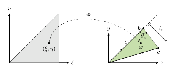
Figure 5: Mapping $\phi$ from the reference triangle $\hat{T}$ to $T_{e}$.

There exists an affine mapping $\bm{\phi}:\widehat{T}\to T_{e}\subset K$, where $\widehat{T}$ is the unit triangle in Lemma 6.1. Without loss of generality, it is assumed that the edge of interest $e$ aligns with $y=x$ in $\mathbb{R}^{2}$, which shares the same tangential direction as the hypotenuse of $\widehat{T}$. One vertex of the edge $e$ is assumed to be the origin (see Figure 5), then:

(6.4) $$\bm{x}=\bm{\phi}(\xi,\eta)=\xi\bm{c}+\eta(\bm{b}-\bm{c}),\text{ for }0\leq\eta\leq\xi\leq 1,$$

where $\bm{b}=h_{e}\langle 1,1\rangle$ and $\bm{c}$ represent the other two vertices. Using the parametrization (6.4): $e\ni\bm{x}=\bm{\phi}(\xi,\xi)=h_{e}\langle\xi,\xi\rangle$ for $0\leq\xi\leq 1$, thus $\,{\rm d}s(\bm{x})=\sqrt{2}\,h_{e}\,{\rm d}\xi$, and the $1/2$-seminorm defined in (2.11) is:

(6.5) $$|v|_{\frac{1}{2},e}^{2}=\int_{(0,1)^{2}}\frac{|v\big{(}\bm{\phi}(t,t)\big{)}-v\big{(}\bm{\phi}(\tau,\tau)\big{)}|^{2}}{2h_{e}^{2}|t-\tau|^{2}}\,2h_{e}^{2}\,\,{\rm d}t\,{\rm d}\tau=|\widehat{v}|_{\frac{1}{2},\hat{e}}.$$

By Lemma 6.1, let the $\widehat{\nabla}$ denote the gradient in $(\xi,\eta)$ on $\widehat{T}$,

$$|v|_{\frac{1}{2},e}^{2}\leq 4\left\|\widehat{\nabla}v\big{(}\bm{\phi}(\xi,\eta)\big{)}\right\|_{0,\hat{T}}^{2}\leq\;4\int_{\hat{T}}\left(|\nabla v|^{2}\left|\partial_{\xi}\bm{\phi}\right|^{2}+|\nabla v|^{2}\left|\partial_{\eta}\bm{\phi}\right|^{2}\right)\,\,{\rm d}\eta\,{\rm d}\xi.$$

One has $|J_{\bm{\phi}}|=2|T_{e}|=h_{e}\,l_{e}$ for the mapping (6.4), and $\left|\partial_{\xi}\bm{\phi}\right|^{2}=|\bm{c}|^{2}$ and $\left|\partial_{\eta}\bm{\phi}\right|^{2}=|\bm{b}-\bm{c}|^{2}$. Inserting these identities into above integral yields:

(6.6) $$|v|_{\frac{1}{2},e}^{2}\leq 4\frac{|\bm{c}|^{2}+|\bm{b}-\bm{c}|^{2}}{|J_{\bm{\phi}}|}\int_{\hat{T}}|{\nabla v}|^{2}|J_{\bm{\phi}}|\,\,{\rm d}\eta\,{\rm d}\xi\lesssim\frac{|\bm{c}|^{2}+|\bm{b}-\bm{c}|^{2}}{|J_{\bm{\phi}}|}|v|_{1,T_{e}}^{2}.$$

As the two angles adjacent to $e$ are nonobtuse, $|\bm{c}|^{2}+|\bm{b}-\bm{c}|^{2}\leq h_{e}^{2}+2l_{e}^{2}$, and (6.2) holds by the following estimate:

$$\left(|\bm{c}|^{2}+|\bm{b}-\bm{c}|^{2}\right)|J_{\bm{\phi}}|^{-1}\lesssim(h_{e}^{2}+l_{e}^{2})/(h_{e}l_{e}).$$

Now when A2 is met with $0<\gamma\leq 1$, we simply let $l_{e}=\gamma h_{e}$, and (6.3) follows.

Lemma 6.4 (a trace inequality for an edge in a polygon).

If on a polygon $K$, an edge $e\subset\partial K$ has the height $l_{e}$ defined in (3.2), and $T_{e}$ is the triangle with base $e$ and height $l_{e}$, then the following trace inequality holds:

(6.7) $$\left\|v\right\|_{0,e}\lesssim l_{e}^{-1/2}\left\|v\right\|_{0,T_{e}}+\bigl{(}l_{e}^{1/2}+l_{e}^{-1/2}h_{e}\bigr{)}\left\|\nabla v\right\|_{0,T_{e}}.$$

Furthermore, if the edge $e$ satisfies A2 with constant $0<\gamma\leq 1$:

(6.8) $$\left\|v\right\|_{0,e}\lesssim\gamma^{-1/2}\left(h_{e}^{-1/2}\left\|v\right\|_{0,K}+h_{e}^{1/2}\left\|\nabla v\right\|_{0,K}\right).$$

Proof 6.5.

Consider a reference triangle $\widehat{T}_{e}$ with base $e$, height of length $h_{e}$, and the two angles adjacent to $e$ being acute. Let the base align with the horizontal $\hat{x}$-axis and choose the origin as the projection of vertex of $T_{e}$ opposite to $e$. It is well known that ([23, Theorem 1.5.1.10], [37, Appendix Lemma A.3]) for any $\widehat{v}\in H^{1}(\widehat{T}_{e})$,

(6.9) $$\left\|\widehat{v}\right\|_{0,e}^{2}\lesssim h_{e}^{-1}\left\|\widehat{v}\right\|_{0,\widehat{T}_{e}}^{2}+h_{e}\bigl{\|}\widehat{\nabla}\widehat{v}\bigr{\|}_{0,\widehat{T}_{e}}^{2}.$$

The mapping $\bm{\psi}:\hat{x}\mapsto x=\hat{x}$, $\hat{y}\mapsto y=l_{e}\hat{y}/h_{e}$ maps $\widehat{T}_{e}$ to $T_{e}$, which has base length $h_{e}$ and height $l_{e}$. Equation (6.7) follows from a straightforward change of variable computation:

(6.10) $$\left\|v\right\|_{0,e}^{2}=\left\|\widehat{v}\right\|_{0,e}^{2}\lesssim l_{e}^{-1}\left\|v\right\|_{0,T_{e}}^{2}+h_{e}^{2}l_{e}^{-1}\left\|\partial_{x}v\right\|_{0,T_{e}}^{2}+l_{e}\left\|\partial_{y}v\right\|_{0,T_{e}}^{2}.$$

(6.8) then follows from the same argument for (6.3) in the previous lemma:

$$\left\|v\right\|_{0,e} \lesssim(\gamma h_{e})^{-1/2}\left\|v\right\|_{0,T_{e}}+\gamma^{-1/2}h_{e}^{1/2}\left\|\nabla v\right\|_{0,T_{e}}$$

$$\leq\gamma^{-1/2}\left(h_{e}^{-1/2}\left\|v\right\|_{0,K}+h_{e}^{1/2}\left\|\nabla v\right\|_{0,K}\right).$$

Remark 6.6.

A short edge with length $h_{e}\ll h_{K}$ is allowed provided that it satisfies A2. For a long edge that only supports a triangle with a short height, i.e., $l_{e}\ll h_{e}\eqsim h_{K}$, this trace inequality does not imply any meaningful estimate and this is one of the main difficulties for the anisotropic error estimate. $\Box$

Appendix B: Poincaré–Friedrichs Inequalities

In this appendix, we review Poincaré–Friedrichs inequalities with a constant depending only on the diameter of the domain but not on the shape.

Lemma 6.7 (Poincaré inequality with average zero in a convex domain [33]).

Let $K\subset\mathbb{R}^{d}$ be a convex domain with a continuous boundary. For any $v\in H^{1}(K)$,

(6.11) $$\left\|v-\bar{v}^{K}\right\|_{0,K}\leq\frac{h_{K}}{\pi}\left\|\nabla v\right\|_{0,K}.$$

Lemma 6.8 (Poincaré inequality with average zero on a subset).

Let $S\subset\mathbb{R}^{2}$ be a convex domain, and a nondegenerate $\omega\subset S$, then for any $v\in H^{1}(S)$,

(6.12) $$\left\|v-\bar{v}^{\omega}\right\|_{0,S}\leq\left(1+\frac{|S|^{\frac{1}{2}}}{|\omega|^{\frac{1}{2}}}\right)\frac{h_{S}}{\pi}\left\|\nabla v\right\|_{0,S}.$$

Proof 6.9.

A straightforward argument exploiting (6.11) is as follows:

$$\left\|v-\bar{v}^{\omega}\right\|_{0,S}\leq\left\|v-\bar{v}^{S}\right\|_{0,S}+\left\|\bar{v}^{S}-\bar{v}^{\omega}\right\|_{0,S}\leq\frac{h_{S}}{\pi}\left\|\nabla v\right\|_{0,S}+\frac{|S|^{\frac{1}{2}}}{|\omega|^{\frac{1}{2}}}\left\|v-\bar{v}^{S}\right\|_{0,\omega}.$$

Then the estimate (6.12) follows directly from $\left\|v-\bar{v}^{S}\right\|_{0,\omega}\leq\left\|v-\bar{v}^{S}\right\|_{0,S}$ and (6.11).

Lemma 6.10 (Poincaré inequality with average zero on a subset of boundary).

Let $K\subset\mathbb{R}^{2}$ be a Lipschitz polygon and $\Gamma\subset\partial K$ be a connected subset, then for any $v\in H^{1}(K)$ such that $\overline{v}^{\Gamma}=0$, the following inequality holds:

(6.13) $$\left\|v\right\|_{0,\Gamma}\leq h_{\Gamma}^{1/2}|v|_{\frac{1}{2},\Gamma}.$$

Proof 6.11.

First inserting the $\overline{v}^{\Gamma}$ into the $L^{2}$-norm yields:

(6.14) $$\left\|v\right\|_{0,\Gamma}^{2}=\int_{\Gamma}\Bigg{(}\frac{1}{|\Gamma|}\int_{\Gamma}\big{(}v(\bm{x})-v(\bm{y})\big{)}\,{\rm d}s(\bm{y})\Bigg{)}^{2}\,{\rm d}s(\bm{x}).$$

Inserting terms to match the $1/2$-seminorm yields the estimate (6.13):

(6.15) $$\left\|v\right\|_{0,\Gamma}^{2}=\frac{1}{|\Gamma|}\int_{\Gamma}\int_{\Gamma}\frac{\big{|}v(\bm{x})-v(\bm{y})\big{|}^{2}}{|\bm{x}-\bm{y}|^{2}}\cdot|\bm{x}-\bm{y}|^{2}\,\,{\rm d}s(\bm{y})\,{\rm d}s(\bm{x})\leq\frac{\max\limits_{x,y\in\Gamma}|\bm{x}-\bm{y}|^{2}}{|\Gamma|}|v|_{\frac{1}{2},\Gamma}^{2}.$$

;

Lemma 6.12 (Poincaré inequality for continuous and piecewise polynomials in
$|\cdot|_{\frac{1}{2},\mathcal{E}_{K}}$).

Let $K\subset\mathbb{R}^{2}$ be a Lipschitz polygon and $\Gamma\subset\partial K$ be a connected subset; then for any $v\in B_{p}(\partial K)\subset C^{0}(\partial K)$ such that $\overline{v}^{\Gamma}=0$, the following inequality holds:

(6.16) $$\left\|v\right\|_{0,e}\lesssim n_{\mathcal{E}_{K}}^{1/2}h_{e}^{1/2}|v|_{\frac{1}{2},\mathcal{E}_{K}}.$$

Proof 6.13.

First let $v\in B_{1}(\partial K)$, the mean value theorem implies that $v(\bm{\xi})=0$ for some $\bm{\xi}\in\Gamma$. Without loss of generality, $\bm{\xi}$ is assumed to be different with any given vertex on $\partial K$. Denote $\Gamma_{\bm{x}}$ as the curve along $\partial K$ from $\bm{\xi}$ to $\bm{x}$ for any $\bm{x}\in e$:

(6.17) $$v(\bm{x})=\int_{\Gamma_{\bm{x}}}\nabla v\cdot\bm{t}\,\,{\rm d}s\leq\sum_{\begin{subarray}{c}e\subset\partial K,\\ e\cap\Gamma_{\bm{x}}\neq\varnothing\end{subarray}}\int_{e}|\partial_{e}v|\,\,{\rm d}s=\sum_{\begin{subarray}{c}e\subset\partial K,\\ e\cap\Gamma_{\bm{x}}\neq\varnothing\end{subarray}}|v(\bm{b}_{e})-v(\bm{a}_{e})|.$$

As a result, integrating on $e$ yields the estimate (6.16) for $v\in B_{1}(\partial K)$:

(6.18) $$\left\|v\right\|_{0,e}^{2}\leq n_{\mathcal{E}_{K}}\,h_{e}\sum_{\begin{subarray}{c}e^{\prime}\subset\partial K,\\ e^{\prime}\cap\Gamma_{\bm{x}}\neq\varnothing\end{subarray}}\,|v(\bm{b}_{e^{\prime}})-v(\bm{a}_{e^{\prime}})|^{2}=n_{\mathcal{E}_{K}}h_{e}\sum_{e^{\prime}\cap\Gamma\neq\varnothing}|v|_{\frac{1}{2},e^{\prime}}^{2}.$$

Now for $v\in B_{p}(\partial K)$, the point $\bm{\xi}$, where $v$ vanishes, is treated as an artificial new vertex on $\partial K$. With this additional vertex $\bm{\xi}$ on $\partial K$, let $v_{I}\in B_{1}(\partial K)$ be $v$’s linear nodal interpolation, and $\mathcal{E}^{\prime}_{K}$ be the collection of the edges with two new edges, which have $\bm{\xi}$ as an end point, replacing the one edge in $\mathcal{E}_{K}$. Then by a standard Bramble–Hilbert estimate ([20, Proposition 6.1]) and the same argument above for $v_{I}$, it holds that

(6.19) $$\left\|v\right\|_{0,e}\leq\left\|v-v_{I}\right\|_{0,e}+\left\|v_{I}\right\|_{0,e}\lesssim h_{e}^{1/2}|v|_{\frac{1}{2},e}+(n_{\mathcal{E}_{K}}+1)^{1/2}h_{e}^{1/2}|v_{I}|_{\frac{1}{2},\mathcal{E}^{\prime}}.$$

By a standard inverse inequality and the interpolation error estimates,

(6.20) $$|v_{I}|_{\frac{1}{2},\mathcal{E}^{\prime}_{K}}\leq|v|_{\frac{1}{2},\mathcal{E}_{K}^{\prime}}+|v-v_{I}|_{\frac{1}{2},\mathcal{E}^{\prime}_{K}}\lesssim|v|_{\frac{1}{2},\mathcal{E}^{\prime}_{K}}+\left(\sum_{e\in\mathcal{E}^{\prime}_{K}}h_{e}^{-1}\left\|v-v_{I}\right\|_{0,e}^{2}\right)^{1/2}\lesssim|v|_{\frac{1}{2},\mathcal{E}^{\prime}_{K}}.$$

The lemma follows immediately from the fact that $|v|_{\frac{1}{2},\mathcal{E}^{\prime}_{K}}\leq|v|_{\frac{1}{2},\mathcal{E}_{K}}$ by the definition of the $1/2$-seminorm (2.11).

Corollary 6.14 (Equivalence between $\left\|\cdot\right\|_{\infty,\partial K}$ and $|\cdot|_{\frac{1}{2},\mathcal{E}_{K}}$).

The following norm equivalence holds with a constant depending only on $n_{\mathcal{E}_{K}}$ and $p$:

(6.21) $$\left\|v\right\|_{\infty,\partial K}\lesssim|v|_{\frac{1}{2},\mathcal{E}_{K}}\lesssim\left\|v\right\|_{\infty,\partial K},\qquad v\in B_{p}(\partial K),\;\overline{v}^{\partial K}=0.$$

Proof 6.15.

The first inequality is a direct consequence of Lemma 6.12 and a standard inverse estimate on each edge $\left\|v\right\|_{\infty,e}\lesssim h_{e}^{-1/2}\left\|v\right\|_{0,e}$. For the second one, one can use a similar argument with (6.20). Let $v_{I}$ be the linear interpolant of $v$ on $\partial K$

$$|v|_{\frac{1}{2},\mathcal{E}_{K}}\leq|v_{I}|_{\frac{1}{2},\mathcal{E}_{K}}+|v-v_{I}|_{\frac{1}{2},\mathcal{E}_{K}}\lesssim\left\{\sum_{e\subset\partial K}\!\Big{(}|v_{I}(\bm{b}_{e})-v_{I}(\bm{a}_{e})|^{2}+h_{e}^{-1}\left\|v-v_{I}\right\|_{0,e}^{2}\Big{)}\right\}^{1/2}.$$

The corollary follows by $v=v_{I}$ at the vertices, and $h_{e}^{-\frac{1}{2}}\left\|v-v_{I}\right\|_{0,e}\lesssim\left\|v\right\|_{\infty,e}$.

Remark 6.16 (difference between estimates (6.13) and (6.16)).

We remark that for an $H^{\frac{1}{2}}(\partial K)$ function, (6.13) is an estimate in the $1/2$-seminorm on the whole $\partial K$. While for a VEM function which is a piecewise polynomial on $\partial K$, a more delicate Poincaré inequality can be obtained in broken $1/2$-seminorm when the zero average is imposed. $\Box$

For an edge $e\subset\partial K$, construct a trapezoid $K_{e}\subset K$ with base $e$ from $T_{e}$, which is the triangle with height $l_{e}$ defined in (3.2), by connecting the midpoints of the two edges adjacent to $e$ in $T_{e}$. With a slight abuse of notation, we still denote the height of $K_{e}$ as $l_{e}$ for base $e$.

In the following proof, one can always start with a rectangle with side $h_{e}$ and height $l_{e}$. The general trapezoid can be transformed into the square by considering a parametrization (see Figure 3(c)) for a quadrilateral with vertices $\bm{a}_{i}$ ($i=1,\dots,4$). Without loss of generality, $\bm{a}_{1}$ is assumed to be the origin. For any $\bm{x}\in K$, and $(\xi,\eta)\in\widehat{S}:=(0,1)^{2}$, consider the following bilinear mapping $\bm{\psi}:(\xi,\eta)\mapsto\bm{x}$:

(6.22) $$\bm{x}=\bm{\psi}(\xi,\eta)=(1-\xi)\eta\,\bm{a}_{3}+\xi(1-\eta)\,\bm{a}_{2}+\xi\eta\,\bm{a}_{4}.$$

If the two opposite angles, sharing $e$ as one side, are uniformly bounded above and below, and the top edge has comparable length with the base $e$, then it is straightforward to verify that

(6.23) $$\|\partial_{\xi}\bm{x}\|_{\infty,K}\lesssim h_{e},\quad\|\partial_{\eta}\bm{x}\|_{\infty,K}\lesssim l_{e},\quad|J_{\bm{\psi}}|\eqsim l_{e}h_{e}.$$

Lemma 6.17 (Poincaré inequality with average zero on a boundary edge).

Let $K\subset\mathbb{R}^{2}$ be a Lipschitz polygon, and let $e\subset\partial K$ be an edge satisfying the condition: there exists a trapezoid $K_{e}\subset K$ of height $l_{e}$ and base $e$, with two angles adjacent to $e$ uniformly bounded above and below. Then the following inequality holds:

(6.24) $$\left\|v-\overline{v}^{e}\right\|_{0,K_{e}}\lesssim(l_{e}h_{e})^{1/2}|v|_{\frac{1}{2},e}+l_{e}\left\|\nabla v\right\|_{0,K_{e}}.$$

Moreover, if $K$ is convex, then

(6.25) $$\left\|v-\overline{v}^{e}\right\|_{0,K}\lesssim\frac{|K|^{1/2}}{|K_{e}|^{1/2}}\,h_{K}\left\|\nabla v\right\|_{0,K}.$$

Proof 6.18.

Applying the parametrization $\bm{x}=\bm{\psi}(\xi,\eta)$ in (6.22) for any $\bm{x}\in K_{e}$, define $\widehat{v}(\xi,\eta):=v\big{(}\bm{\psi}(\xi,\eta)\big{)}$ for $(\xi,\eta)\in\widehat{S}$. By the fundamental theorem of calculus,

(6.26) $$\widehat{v}(\xi,\eta)-\overline{v}^{e}=\widehat{v}(\xi,0)-\overline{v}^{e}+\int^{\eta}_{0}\partial_{\eta}\widehat{v}(\xi,\tau)\,\,{\rm d}\tau.$$

By the relation (6.23) and Young’s inequality,

$$\left\|v-\overline{v}^{e}\right\|_{0,K}^{2}\lesssim l_{e}h_{e}\left\|\widehat{v}-\overline{v}^{e}\right\|_{0,\widehat{S}}^{2}\lesssim l_{e}h_{e}\left(\left\|\widehat{v}-\overline{v}^{e}\right\|_{0,\hat{e}}^{2}+\|\partial_{\eta}\widehat{v}\|_{0,\widehat{S}}^{2}\right),$$

where $\hat{e}=\{\xi\in(0,1),\eta=0\}$ is the pre-image of $e$ in the reference square. Using (6.23) and Poincaré inequality (6.24), the first term can be bounded by

$$h_{e}\left\|\widehat{v}-\overline{v}^{e}\right\|_{0,\hat{e}}^{2}=\left\|v-\overline{v}^{e}\right\|_{0,e}^{2}\leq h_{e}|v|_{\frac{1}{2},e}^{2}.$$

The estimate (6.24) then follows from:

$$l_{e}h_{e}\|\partial_{\eta}\widehat{v}\|_{0,S}^{2}\lesssim\int_{S}|\nabla v(\bm{x})|^{2}|\partial_{\eta}\bm{x}|^{2}|J_{\bm{\psi}}|\,{\rm d}\xi\,{\rm d}\eta\lesssim l_{e}^{2}\,\|\nabla v\|_{0,K_{e}}^{2}.$$

To obtain (6.25), one can apply the trace inequality (6.2) to get

(6.27) $$\left\|v-\overline{v}^{e}\right\|^{2}_{0,K_{e}}\lesssim l_{e}h_{e}|v|_{\frac{1}{2},e}^{2}+l_{e}^{2}\left\|\nabla v\right\|_{0,K_{e}}^{2}\lesssim(l_{e}+h_{e})^{2}\|\nabla v\|_{0,K}^{2}.$$

To bridge the inequality from $K_{e}$ to $K$, using the triangle inequality, Poincaré inequality (6.11), $h_{e}\eqsim h_{K},l_{e}\leq h_{K}$, and the estimate above yield

$$\left\|v-\overline{v}^{e}\right\|_{0,K} \leq\left\|v-\overline{v}^{K}\right\|_{0,K}+\left\|\overline{v}^{K}-\overline{v}^{K_{e}}\right\|_{0,K}+\left\|\overline{v}^{K_{e}}-\overline{v}^{e}\right\|_{0,K}$$

$$\lesssim h_{K}\left\|\nabla v\right\|_{0,K}+\frac{|K|^{1/2}}{|K_{e}|^{1/2}}\left(\left\|v-\overline{v}^{K}\right\|_{K_{e}}+\left\|v-\overline{v}^{e}\right\|_{K_{e}}\right)$$

(6.28) $$\lesssim\frac{|K|^{1/2}}{|K_{e}|^{1/2}}\,h_{K}\left\|\nabla v\right\|_{0,K}.$$

References

- [1] G. Acosta and R. G. Durán, Error estimates for isoparametric elements satisfying a weak angle condition, SIAM J. Numer. Anal., 38 (2000), pp. 1073–1088.
- [2] B. Ahmad, A. Alsaedi, F. Brezzi, L. D. Marini, and A. Russo, Equivalent projectors for virtual element methods, Comp. Math. Appl., 66 (2013), pp. 376–391.
- [3] B. Ayuso de Dios, K. Lipnikov, and G. Manzini, The nonconforming virtual element method, ESAIM: Math. Model. Numer. Anal., 50 (2016), pp. 879–904.
- [4] I. Babuška and A. K. Aziz, On the angle condition in the finite element method, SIAM J. Numer. Anal., 13 (1976), pp. 214–226.
- [5] L. Beirão da Veiga, F. Brezzi, A. Cangiani, G. Manzini, L. Marini, and A. Russo, Basic principles of virtual element methods, Math. Models Methods Appl. Sci., 23 (2013), pp. 199–214.
- [6] L. Beirão da Veiga, F. Dassi, and A. Russo, High-order virtual element method on polyhedral meshes, Comp. Math. Appl., 74 (2017), pp. 1110–1122.
- [7] L. Beirão da Veiga, C. Lovadina, and A. Russo, Stability analysis for the virtual element method, Math. Models Methods Appl. Sci., 27 (2017), pp. 2557–2594.
- [8] M. F. Benedetto, S. Berrone, S. Pieraccini, and S. Scialò, The virtual element method for discrete fracture network simulations, Comp. Methods Appl. Mech. Engrg., 280 (2014), pp. 135–156.
- [9] S. Berrone and A. Borio, Orthogonal polynomials in badly shaped polygonal elements for the virtual element method, Finite Elem. Anal. Des., 129 (2017), pp. 14–31.
- [10] S. C. Brenner and L.-Y. Sung, Virtual element methods on meshes with small edges or faces, Math. Models Methods Appl. Sci., 28 (2018), pp. 1291–1336.
- [11] F. Brezzi, A. Buffa, and K. Lipnikov, Mimetic finite differences for elliptic problems, ESAIM: Math. Model. Numer. Anal., 43 (2009), pp. 277–295.
- [12] F. Brezzi, The great beauty of VEMs, Proceedings of the ICM, 1 (2014), pp. 217–235.
- [13] E. Burman and P. Hansbo, Fictitious domain finite element methods using cut elements: I. a stabilized lagrange multiplier method, Comp. Methods Appl. Mech. Engrg., 199 (2010), pp. 2680–2686.
- [14] W.-M. Cao and B. Guo, Preconditioning for the p-version boundary element method in three dimensions with triangular elements, J. Korean Math. Soc., 41 (2004), pp. 345–368.
- [15] S. Cao and L. Chen, Anisotropic error estimates of the linear nonconforming virtual element methods, arXiv preprint arXiv:1806.09054, (2018).
- [16] S. Cao, L. Chen and F. Lin, A note on the error estimate of the virtual element methods, arXiv preprint arXiv:1810.00926, (2018).
- [17] L. Chen and J. Huang, Some error analysis on virtual element methods, Calcolo, 55 (2018), p. 5.
- [18] L. Chen, H. Wei, and M. Wen, An interface-fitted mesh generator and virtual element methods for elliptic interface problems, J. Comput. Phys., 334 (2017), pp. 327–348.
- [19] Q. Du, V. Faber, and M. Gunzburger, Centroidal voronoi tessellations: Applications and algorithms, SIAM Rev., 41 (1999), pp. 637–676.
- [20] T. Dupont and R. Scott, Polynomial approximation of functions in Sobolev spaces, Math. Comp., 34 (1980), pp. 441–463.
- [21] R. G. Durán, Error estimates for 3–D narrow finite elements, Math. Comp., 68 (1999), pp. 187–199.
- [22] A. Ern and J.-L. Guermond, Finite element quasi-interpolation and best approximation, ESAIM: Math. Model. Numer. Anal., 51 (2017), pp. 1367–1385.
- [23] P. Grisvard, Elliptic Problems in Nonsmooth Domains, Classics Appl. Math. 69, SIAM, Philadelphia, PA, 1985.
- [24] A. Hannukainen, S. Korotov, and M. Křížek, The maximum angle condition is not necessary for convergence of the finite element method, Numer. Math., 120 (2012), pp. 79–88.
- [25] M. Křížek, On semiregular families of triangulations and linear interpolation, Appl. Math., 36 (1991), pp. 223–232.
- [26] M. Křížek, On the maximum angle condition for linear tetrahedral elements, SIAM J. Numer. Anal., 29 (1992), pp. 513–520.
- [27] J. L. Lions and E. Magenes, Non-homogeneous boundary value problems and applications, Grundlehren Math. Wiss. 181, Springer, Cham, 2012.
- [28] L. Mascotto, Ill-conditioning in the virtual element method: stabilizations and bases, Numer. Methods Partial Differential Equation, 34 (2018), pp. 1258–1281.
- [29] L. Mascotto and F. Dassi, Exploring high-order three dimensional virtual elements: bases and stabilizations, Comp. Math. Appl., 75 (2018), pp. 3379–3401.
- [30] D. Mora, G. Rivera, and R. Rodríguez, A virtual element method for the Steklov eigenvalue problem, Math. Models Methods Appl. Sci., 25 (2015), pp. 1421–1445.
- [31] J. Nečas, Les methodes directes en theorie des equations elliptiques., Masson et Cie, Academia, 1967.
- [32] G. H. Paulino, A. L. Gain, Bridging art and engineering using Escher-based virtual elements, Struct. Multidiscip. Optim., 51(4) (2015), pp. 867–883.
- [33] L. E. Payne and H. F. Weinberger, An optimal poincaré inequality for convex domains, Arch. Ration. Mech. Anal., 5 (1960), pp. 286–292.
- [34] N. A. Shenk, Uniform error estimates for certain narrow Lagrangian finite elements, Math. Comp., 63 (1994), pp. 105–119.
- [35] E. M. Stein, Singular Integrals and Differentiability Properties of Functions, Princeton Math. Ser. 30, Princeton University Press, Princeton, NJ, 1970.
- [36] C. Talischi, G. H. Paulino, A. Pereira, and I. F. Menezes, Polymesher: a general-purpose mesh generator for polygonal elements written in MATLAB, Struct. Multidiscip. Optim., 45 (2012), pp. 309–328.
- [37] J. Wang and X. Ye, A weak Galerkin mixed finite element method for second order elliptic problems, Math. Comp., 83 (2014), pp. 2101–2126.
- [38] P. Wriggers, W. Rust, and B. Reddy, A virtual element method for contact, Comput. Mech., 58 (2016), pp. 1039–1050.
- [39] J. Xu and J. Zou, Some nonoverlapping domain decomposition methods, SIAM Rev., 40 (1998), pp. 857–914.